Abstract
This paper explores the exact solutions of the fractional Hirota–Satsuma coupled KdV (fHScKdV) equation in the Beta fractional derivative. The logistic method is first proposed to construct analytical solutions for the fHScKdV equation. In order to better comprehend the physical structure of the solutions, three-dimensional visualizations and line graphs of the exponent function solutions are depicted with the aid of Matlab. Furthermore, the phase portraits and bifurcation behaviors of the fHScKdV model under transformation are studied. Sensitivity and chaotic behaviors are analyzed in specific conditions. The phase plots and time series map are exhibited through sensitivity analysis and perturbation factors. These investigations enhance our understanding of practical phenomena governed by the fHScKdV model, and are crucial for examining the dynamic behaviors and phase portraits of the fHScKdV system. The strategies utilized here are more direct and effective, and can be applied effortlessly to other fractional order differential equations.
1. Introduction
Due to the inherent complexity of various phenomena, linear systems are often theoretical approximating of simpler nonlinear systems. However, nonlinear systems more accurately capture the essence of the objective world. Therefore, comprehending and studying nonlinear phenomena is crucial for modern science and technology. From a mathematical physics standpoint, numerous nonlinear phenomena can be reduced to solve nonlinear differential equations [1,2,3]. Among these, nonlinear fractional differential equations (NLFDEs) have garnered considerable attention. NLFDEs represent an extension of partial differential equations in which the order of derivatives can be fractional rather than integer-valued. These equations have significant applications in physics, engineering, biology, finance, and numerous other fields, particularly in describing systems with memory effects, nonlocal phenomena, or complex dynamics. NLFDEs typically involve fractional derivatives with respect to spatial or temporal variables. Fractional derivatives can be defined in several ways, the most common of which are the Caputo [4], Grünwald–Letnikov [5], Riemann–Liouville [6] and Beta [7] definitions. NLFDEs symbolise a vibrant research field that provides powerful tools in describing the dynamics of complex systems. As computational methods and theories continue to evolve, we can see that even more novel applications and solution techniques are emerging for NLFDEs.
In the literature, many effective approaches have been constructed to search analytical solutions of NLFDEs, such as the F-expansion method [8], the fractional sub-equation method [9,10,11], the generalized Riccati equation mapping method [12], the first integral method [13,14], the Kudryashov methods [15,16], the -expansion method [17,18], the -expansion method [19,20,21,22], the tanh-function method [23,24], the modified simple equation method [25,26,27], the truncated Painlevé expansion method [23], the Sine–Gordon expansion method [28], the complex method [29,30,31] and so on.
The HScKdV equation [32] typically describes the interaction between two long waves and different dispersion relations. By extending it to the fractional form, the fHScKdV equation captures additional layers of complexity that cannot be fully captured by integer-order derivatives. The fHScKdV equation [33] is given as follows:
where denotes the Beta differential operator.
The fHScKdV equation has potential applications in various fields, including physics, engineering, and finance. For example, in fluid mechanics, it can be used to model wave and turbulence phenomena with fractional properties. In materials science, it can describe the behavior of materials with memory effects. In finance, it can analyze market dynamics, exhibiting long-memory effects. The fHScKdV equation is an interesting system that attracts researchers to analyze it in depth. Alam et al. [33] acquired the closed-form solutions using the -expansion method as well as the Riemann–Liouville derivative. Yin et al. [34] utilized the homogeneous balance method, improved F-expansion method, and unified method, and extracted various analytical solutions. Ganji et al. [35] exploited the homotopy perturbation method to obtain exact solutions. Yan [36] constructed exact doubly periodic solutions by applying the extended Jacobian elliptic function expansion technique. Kaplan and Bekir [37] applied the -expansion method and local fractional derivatives to derived exact solutions for the fHScKdV equation. They were all committed to using effective methods to quickly obtain solutions to nonlinear differential equations. Inspired by these studies, we put forward the logistic approach, which is founded on the notion that the precise solutions of a nonlinear differential equation can be expounded by a polynomial in , and complies with the logistic ordinary differential equation. Our results indicate that the logistic method is direct and effective. This enriches the study of the fHScKdV equation and may provide reference for researchers in related fields. In this paper, we propose a new approach, named the logistic method, to study the fHScKdV equation, and investigate its bifurcation, sensitivity and chaotic behaviors.
The paper is organized as follows. The logistic method is introduced in Section 2 to execute analytical solutions of the fHScKdV equation. Section 3 extracts solutions to the fHScKdV equation, and shows the dynamic behaviors of these solutions in 3D, contour plot and line plots. Phase portraits and bifurcation behavior analysis of the fHScKdV system are presented in Section 4. In Section 5, sensitivity analysis to the initial value is explained. The chaotic behavior regarding the fHScKdV equation is interpreted in Section 6. The conclusions are given in Section 7.
2. Proposal of the Logistic Method
Recently, the Beta fractional derivative (FD) concept was put forward by some researchers [38], signifying significant progress in the study of mathematical derivatives. In particular, Beta FD has a stronger ability to precisely predict real-time phenomena compared to the standard derivative. The key advantage of FD is its non-locality, which reveals the effect of distant elements on the behavior of a system and brings fundamental value. A wide range of fields, like dielectric polarization, viscoelasticity, electrochemistry, and image processing, extensively employ Beta FD. Most of these applications are in engineering and physics, for instance wave theory, biotechnology, mass transfer, heat, robotics, and so on.
First, some definitions of the Beta fractional derivative are introduced and a detailed explanation of the logistic method is given to better elucidate the obtained results.
Let be specified as a function of all non-negative z with the derivative [39,40], hence
in which is the Gamma function. Some effective properties [39,40,41,42] of the above definition are included:
Using this knowledge about Beta derivatives, analytical solutions of the fHScKdV equation are sought by exerting the logistic method, which is presented according to the following steps.
Consider a space-time NLFDE as follows:
where F is the polynomial of unknown function u with its fractional derivatives and means .
Mechanism I. Inserting the transformation
into space-time NLFDE (5), we yield
where , and P is the polynomial of u along with its derivatives.
Mechanism II. Assume that Equation (7) has the following solution:
where for are constants, and satisfies the following logistic equation:
Mechanism III. At this step, impose the homogeneous balancing method on the highest order derivative of U and highest order nonlinear term in Equation (7), and we can gain the integer n of (8). Apply (8) and Equation (9) to Equation (7), and then we are able to acquire an algebra system through the gathering N with the same order. Utilizing the results of the algebra system, we can obtain the values of and related restriction conditions.
3. Applications to the fHScKdV Equation
We start with the application of the following transform to (1):
By combining the first and second equations of (12), and eliminating , we arrive at
To seek nontrivial solutions, we proceed by reducing the fHScKdV equation to the following ordinary differential equation:
By balancing between and in Equation (14), then can be determined for (8), which yields the solution of U, as follows:
where is satisfied (9). To gain meaningful solutions, displacing (15) along with Equation (9) into Equation (14), we can collect coefficients of the same order of to zero. The algebraic system is attained as below:
and the results produced for coefficients are as below.
Set 1:
Set 2:
By inserting these results into (15) and using the definition of N, the following solutions are extracted for Equation (1).
Case 1:
with
Case 2:
where
Matlab is a powerful software developed by MathWorks, designed for numerical computing, data analysis, algorithm development, and visualization. With the help of Matlab (Version 9.14.0.2306882 (R2023a)), we can reveal the physics performance by presenting the simulations. Since , and are based on the function and are similar to each other, we have only shown the simulation of . We are particularly interested in the impact of the fractional derivative on the function.
To describe the effect of , we set the parameters , , and , while varying the value of from 1 to . The graphs of are depicted in Figure 1 and Figure 2, respectively. In Figure 1a–e, the behaviors of are illustrated for values of , and , respectively. The characteristics at for various values of are shown in Figure 1f. Similarly, uses the same parameters as , and the corresponding plots are shown in Figure 2a–f.
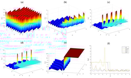
Figure 1.
(a–f) at ; (a) ; (b) ; (c) ; (d) ; (e) ; (f) .
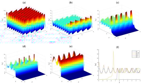
Figure 2.
(a–f) at ; (a) ; (b) ; (c) ; (d) ; (e) ; (f) .
Figure 1a–e and Figure 2a–e clearly demonstrate that as decreases, the region for is compressed into a constant value, and a jump region gradually forms near . Additionally, based on Figure 1a,b and Figure 2a,b, even a slight deviation of from 1 disrupts the original periodicity. These findings play a significant role in the study and analysis of the dynamic behavior of the fHScKdV system. The choice of affects the nonlinear properties of the function, altering its smoothness near . Therefore, it is crucial to carefully consider the impact of the fractional order when studying related systems. Furthermore, these properties may potentially characterize tsunami; however, further research is still needed.
4. Phase Portraits and Bifurcation Behaviors
The Hamiltonian of system (21) is
The system (21) has three equilibrium points:
The Jacobian of (21) is
Then, we have
For the equilibrium point E of a Hamiltonian system, E can be analyzed in three situations: when , E is a center; when , E is a cuspid; and when , E is a saddle. Hence, we conclude that the bifurcation behavior of system (21) is as follows:
Case I: If , is a saddle and are center.
Case II: If , is a center and are saddle.
To analyze system (21), we list the effect of bifurcation by plotting the phase portraits of the system in Figure 3. Case I is shown in Figure 3a by letting the value of the system parameter , while Figure 3b depicts case II by setting the value of system parameter . From Figure 3, we can study the bifurcation behaviors when the values of parameters alter. Therefore, the dynamics behaviors are remarkably affected by the bifurcations.
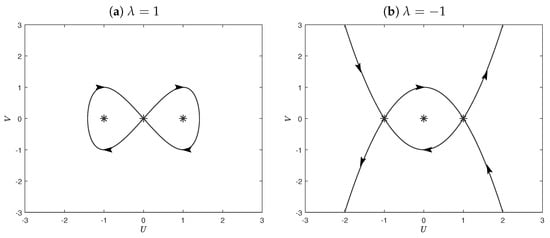
Figure 3.
Phase portraits of case I (a) and case II (b). The stars represent the equilibriums.
5. Sensitive Analysis
Sensitivity analysis pertains to the examination of how a system’s response is sensitive to alterations in parameters or initial conditions. It represents a mathematical method for evaluating the influence of variations within a variable framework on its output. Comprehending the capability and dependability of dynamic structures is of utmost significance. This type of analysis is frequently utilized to explore the changes in configurations or variables that impact the performance of systems in various disciplines like dynamical frameworks and energy.
We examined the sensitivity behaviors of Equation (14) concerning the initial values of cases I and II, as previously discussed. The results for the parameter according to case I are illustrated in Figure 4, while Figure 5 shows the outcomes for case II. In Figure 4 and Figure 5, the red curve represents the initiation at , and the blue curve represents the initiation at . Figure 4a and Figure 5a exhibit the time series for the model (21). In addition, Figure 4b and Figure 5b display phase portraits of system (21) initiated from two distinct initial conditions, highlighting sensitivity impacts. To evaluate the impact of sensitivity variations, we undertook a comparative analysis of the pathways emanating from diverse initial conditions, specifically focusing on the distinguishing patterns between the blue and red curves presented in Figure 4a,b and Figure 5a,b. The results indicate that significant changes in initial conditions have a considerable impact on the dynamic behavior of the system when the remaining parameters remain constant. Moreover, we investigated the system’s sensitivity to parameter variations by comparing Figure 4a,b with Figure 5a,b, demonstrating a significant sensitivity of the system to alterations in its parameters.
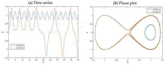
Figure 4.
Sensitivity analysis of case I.
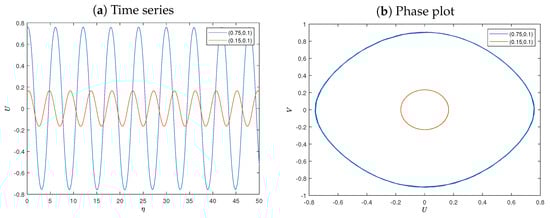
Figure 5.
Sensitivity analysis of case II.
6. Chaotic Behavior
Chaos, in the realm of science and mathematics, refers specifically to the highly complex and completely unpredictable behavior that can be observed within nonlinear systems. This concept implies a state in which the patterns and outcomes are not straightforward or easily foreseen, presenting a level of intricacy that makes it extremely challenging to accurately predict or understand the subsequent developments in such systems. Through the study of chaotic phenomena, we can acquire comprehension of the nonlinear characteristics of the fHScKdV equation and disclose their intricate temporal evolution courses. It is of great significance to consider the dynamic behaviors of system (14) in this paper.
In this segment, our primary concern is the chaotic dynamics exhibited by Equation (14) when subjected to noise-induced perturbations. We undertook an analysis of the chaotic nature of Equation (14) by contemplating a periodic perturbation model as a framework for our discussion. The model is read as:
where and denote the frequency and amplitude of noise, respectively. Equation (26) is an exact forced non-linear pendulum. There have been many similar studies, such as Neishtadt et al.’s [43] study on the dynamics of nonlinear pendulums under periodic forces with small amplitudes and slowly decreasing frequencies. Bazzani et al. [44] applied the perturbative techniques to Hamiltonians. We analyzed the sensitivity of the noise as follows. When either the amplitude or frequency was fixed and the other one varied, we studied the time series as well as phase portraits of the system (21). To study the effect of amplitude , frequency was fixed; the time series and phase portraits are shown in Figure 6 and Figure 7. Similarly, we discuss the impacts of frequency when amplitude is fixed. The results are shown in Figure 8 and Figure 9. In addition, parameter is fixed as in Figure 6 and Figure 8, while is set in Figure 7 and Figure 9.
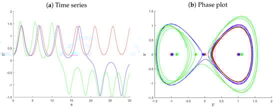
Figure 6.
Chaotic behavior analysis and the amplitude for case I.
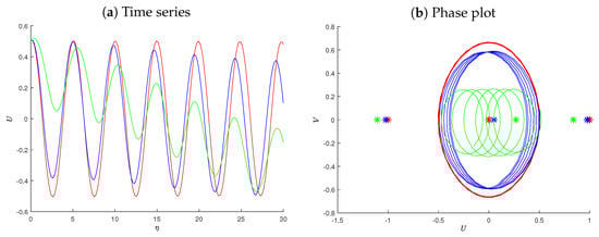
Figure 7.
Chaotic behavior analysis and amplitude for case II.
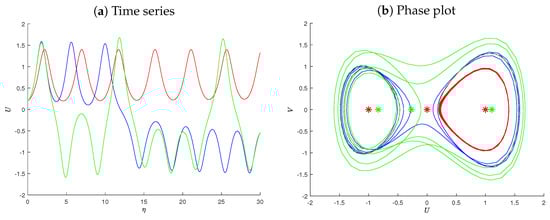
Figure 8.
Chaotic behavior analysis and frequency for case I.
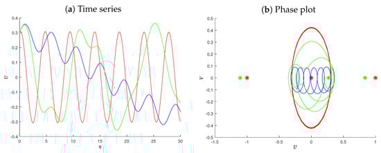
Figure 9.
Chaotic behavior analysis and frequency for case II.
We valued the parameters and as follows. In Figure 6 and Figure 7, we kept and let . The red curve represents the simulation results for the time series and phase orbits. Then, we adjusted to and ; the graphical depiction of the simulation outcomes is distinctively presented via the blue and green lines, respectively. The simulation highlights a pivotal observation: the divergence between the red line and the aforementioned curves underscores the emergence of chaotic system dynamics contingent upon the presence of noise. Notably, in both scenarios under consideration, the system manifests a pronounced sensitivity to variations in the amplitude parameter .
In Figure 8 and Figure 9, we set to 0. The red curve illustrates the simulation results for both the time series and phase orbits. We then adjusted to and to and , with the results represented by the blue and green curves, respectively. The distinction between the red curve and the others indicates that the system exhibits chaotic behavior while the noise term is present. In both cases, the system’s sensitivity to the frequency is significant.
7. Conclusions
In this paper, a transformation using the function is applied to simplify fractional differential equations into ordinary differential equations. The exact solutions of the fHScKdV equation are constructed by proposing and utilizing the logistic method. These derived solutions enable valuable understanding of the inherent physical phenomena in such systems. Furthermore, three-dimensional visualizations and line graphs are presented to depict the influence of different -order derivatives on solutions. By analyzing the plots, we conclude that the choice of has a significant impact on the function. Therefore, the careful selection of is essential in related research. Additionally, we studied the phase portraits and bifurcation behaviors of the fHScKdV model under wave transformation, examining the related sensitivity as well as chaotic behaviors. These investigations not only augment existing knowledge but also shed invaluable light on the intricate dynamics that govern the system, offering fresh insights for further exploration and understanding.
Author Contributions
Conceptualization, Y.G.; Methodology, C.J.; Software, Y.L.; Validation, Y.L.; Writing—original draft, Y.G. and Y.L.; Writing—review and editing, C.J.; Supervision, Y.G. and C.J. All authors have read and agreed to the published version of the manuscript.
Funding
This research is supported by the NSFC (11901111), Science Research Group Project of SEIG (ST202101) and Science Research Project of SEIG (ky202211).
Data Availability Statement
All data were contained in the main text.
Conflicts of Interest
The authors declare no conflicts of interest.
References
- Ullah, M.S.; Ali, M.Z.; Roshid, H.-O.; Seadawy, A.; Baleanu, D. Collision phenomena among lump, periodic and soliton solutions to a (2+1)-dimensional bogoyavlenskii’s breaking soliton model. Phys. Lett. A 2021, 397, 127263. [Google Scholar] [CrossRef]
- Wu, X.-S.; Liu, J.-G. Solving the variable coefficient nonlinear partial differential equations based on the bilinear residual network method. Nonlinear Dyn. 2024, 112, 8329–8340. [Google Scholar] [CrossRef]
- Kumar, D.; Seadawy, A.R.; Haque, M.R. Multiple soliton solutions of the nonlinear partial differential equations describing the wave propagation in nonlinear low-pass electrical transmission lines. Chaos Solitons Fractals 2018, 115, 62–76. [Google Scholar] [CrossRef]
- Tuan, N.H.; Mohammadi, H.; Rezapour, S. A mathematical model for COVID-19 transmission by using the Caputo fractional derivative. Chaos Solitons Fractals 2020, 140, 110107. [Google Scholar] [CrossRef]
- Machado, J.A.T. The bouncing ball and the Grünwald-Letnikov definition of fractional derivative. Fract. Calc. Appl. Anal. 2021, 24, 1003–1014. [Google Scholar] [CrossRef]
- Hilfer, R. Fractional diffusion based on Riemann-Liouville fractional derivatives. J. Phys. Chem. B 2000, 104, 3914–3917. [Google Scholar] [CrossRef]
- Bagheri, M.; Khani, A. Analytical method for solving the fractional order generalized KdV equation by a Beta-fractional derivative. Adv. Math. Phys. 2020, 2020, 8819183. [Google Scholar] [CrossRef]
- Ozkan, E.M. New exact solutions of some important nonlinear fractional partial differential equations with beta derivative. Fractal Fract. 2022, 6, 173. [Google Scholar] [CrossRef]
- Tang, B.; He, Y.; Wei, L.; Zhang, X. A generalized fractional sub-equation method for fractional differential equations with variable coefficients. Phys. Lett. A 2012, 376, 2588–2590. [Google Scholar] [CrossRef]
- Bekir, A.; Aksoy, E.; Cevikel, A. Exact solutions of nonlinear time fractional partial differential equations by sub-equation method. Math. Methods Appl. Sci. 2014, 38, 2779–2784. [Google Scholar] [CrossRef]
- Nisar, K.S.; Inan, I.E.; Inc, M.; Rezazadeh, H. Properties of some higher-dimensional nonlinear schrödinger equations. Results Phys. 2021, 31, 105073. [Google Scholar] [CrossRef]
- Khater, M.M.A.; Jhangeer, A.; Rezazadeh, H.; Akinyemi, L.; Akbar, M.A.; Inc, M. Propagation of new dynamics of longitudinal bud equation among a magneto-electro-elastic round rod. Mod. Phys. Lett. B 2021, 35, 2150381. [Google Scholar] [CrossRef]
- Mirzazadeh, M.; Eslami, M.; Biswas, A. Solitons and periodic solutions to a couple of fractional nonlinear evolution equations. Pramana 2014, 82, 465–476. [Google Scholar] [CrossRef]
- Eslami, M.; Fathi-Vajargah, B.; Mirzazadeh, M.; Biswas, A. Application of first integral method to fractional partial differential equations. Indian J. Phys. 2014, 88, 177–184. [Google Scholar] [CrossRef]
- Hosseini, K.; Mirzazadeh, M.; Baleanu, D.; Raza, N.; Park, C.; Ahmadian, A.; Salahshour, S. The generalized complex Ginzburg-Landau model and its dark and bright soliton solutions. Eur. Phys. J. Plus 2021, 136, 709. [Google Scholar] [CrossRef]
- Hosseini, K.; Mirzazadeh, M.; Salahshour, S.; Baleanu, D.; Zafar, A. Specific wave structures of a fifth-order nonlinear water wave equation. J. Ocean Eng. Sci. 2022, 7, 462–466. [Google Scholar] [CrossRef]
- Kaplan, M.; Bekir, A. A novel analytical method for time-fractional differential equations. Optik 2016, 127, 8209–8214. [Google Scholar] [CrossRef]
- Hosseini, K.; Bekir, A.; Ansari, R. Exact solutions of nonlinear conformable time-fractional boussinesq equations using the exp(-φ(ϵ))-expansion method. Opt. Quantum Electron. 2017, 49, 131. [Google Scholar] [CrossRef]
- Khan, K.; Akbar, M.A.; Koppelaar, H. Study of coupled nonlinear partial differential equations for finding exact analytical solutions. R. Soc. Open Sci. 2015, 2, 140406. [Google Scholar] [CrossRef]
- Zafar, A.; Raheel, M.; Asif, M.; Hosseini, K.; Mirzazadeh, M.; Akinyemi, L. Some novel integration techniques to explore the conformable m-fractional schrödinger-hirota equation. J. Ocean Eng. Sci. 2022, 7, 337–344. [Google Scholar] [CrossRef]
- Nisar, K.S.; Ali, K.K.; Inc, M.; Mehanna, M.S.; Rezazadeh, H.; Akinyemi, L. New solutions for the generalized resonant nonlinear schrödinger equation. Results Phys. 2022, 33, 105153. [Google Scholar] [CrossRef]
- Nisar, K.S.; Inan, I.E.; Yepez-Martinez, H.; Inc, M. Some new type optical and the other soliton solutions of coupled nonlinear hirota equation. Results Phys. 2022, 35, 105388. [Google Scholar] [CrossRef]
- Hu, H.; Li, X. New interaction solutions of the similarity reduction for the integrable (2+1)-dimensional boussinesq equation. Int. J. Mod. Phys. B 2022, 36, 2250001. [Google Scholar] [CrossRef]
- Raslan, K.R.; Ali, K.K.; Shallal, M.A. The modified extended tanh method with the riccati equation for solving the space-time fractional EW and MEW equations. Chaos Solitons Fractals 2017, 103, 404–409. [Google Scholar] [CrossRef]
- Kaplan, M.; Bekir, A.; Akbulut, A.; Aksoy, E. The modified simple equation method for nonlinear fractional differential equations. Rom. J. Phys. 2015, 60, 1374. [Google Scholar]
- Kaplan, M.; Koparan, M.; Bekir, A. Regarding on the exact solutions for the nonlinear fractional differential equations. Open Phys. 2016, 14, 478–482. [Google Scholar] [CrossRef]
- Rahman, Z.; Abdeljabbar, A.; Harun-Or-Roshid; Ali, M.Z. Novel precise solitary wave solutions of two time fractional nonlinear evolution models via the MSE scheme. Fractal Fract. 2022, 6, 444. [Google Scholar] [CrossRef]
- Kumar, D.; Hosseini, K.; Kaabar, M.K.A.; Kaplan, M.; Salahshour, S. On some novel solution solutions to the generalized Schrödinger-Boussinesq equations for the interaction between complex short wave and real long wave envelope. J. Ocean Eng. Sci. 2022, 7, 353–362. [Google Scholar] [CrossRef]
- Gu, Y.; Yuan, W.; Aminakbari, N.; Lin, J. Meromorphic solutions of some algebraic differential equations related Painlevé equation IV and its applications. Math. Methods Appl. Sci. 2018, 41, 3832–3840. [Google Scholar] [CrossRef]
- Gu, Y.; Wu, C.; Yao, X.; Yuan, W. Characterizations of all real solutions for the KdV equation and WR. Appl. Math. Lett. 2020, 107, 106446. [Google Scholar] [CrossRef]
- Gu, Y.; Liao, L. Closed form solutions of Gerdjikov-Ivanov equation in nonlinear fiber optics involving the beta derivatives. Int. J. Mod. Phys. B 2022, 36, 2250116. [Google Scholar] [CrossRef]
- Hirota, R.; Satsuma, J. Soliton solutions of a coupled Korteweg-de Vries equation. Phys. Lett. A 1981, 85, 407–408. [Google Scholar] [CrossRef]
- Alam, M.N.; Seadawy, A.R.; Baleanu, D. Closed-form wave structures of the space-time fractional Hirota-Satsuma coupled KdV equation with nonlinear physical phenomena. Open Phys. 2020, 18, 555–565. [Google Scholar] [CrossRef]
- Yin, Q.; Gao, B. New solutions of the time-fractional Hirota-Satsuma coupled KdV equation by three distinct methods. Int. J. Geom. Methods Mod. Phys. 2023, 20, 2350170. [Google Scholar] [CrossRef]
- Kurt, A.; Rezazadeh, H.; Senol, M.; Neirameh, A.; Tasbozan, O.; Eslami, M.; Mirzazadeh, M. Two effective approaches for solving fractional generalized Hirota-Satsuma coupled KdV system arising in interaction of long waves. J. Ocean Eng. Sci. 2019, 4, 24–32. [Google Scholar] [CrossRef]
- Yan, Z. The extended jacobian elliptic function expansion method and its application in the generalized Hirota-Satsuma coupled KdV system. Chaos Solitons Fractals 2003, 15, 575–583. [Google Scholar] [CrossRef]
- Kaplan, M.; Bekir, A. Construction of exact solutions to the space-time fractional differential equations via new approach. Optik 2017, 132, 1–8. [Google Scholar] [CrossRef]
- Atangana, A.; Baleanu, D.; Alsaedi, A. Analysis of time-fractional hunter-saxton equation: A model of neumatic liquid crystal. Open Phys. 2016, 14, 145–149. [Google Scholar] [CrossRef]
- Atangana, A.; Goufo, E.F.D. Extension of matched asymptotic method to fractional boundary layers problems. Math. Probl. Eng. 2014, 2014, e107535. [Google Scholar] [CrossRef]
- Atangana, A.; Alqahtani, R.T. Modelling the spread of river blindness disease via the Caputo fractional derivative and the beta-derivative. Entropy 2016, 18, 40. [Google Scholar] [CrossRef]
- Hosseini, K.; Mirzazadeh, M.; Gómez-Aguilar, J.F. Soliton solutions of the Sasa-Satsuma equation in the monomode optical fibers including the beta-derivatives. Optik 2020, 224, 165425. [Google Scholar] [CrossRef]
- Hosseini, K.; Kaur, L.; Mirzazadeh, M.; Baskonus, H.M. 1-Soliton solutions of the (2+1)-dimensional Heisenberg ferromagnetic spin chain model with the beta time derivative. Opt. Quantum Electron. 2021, 53, 125. [Google Scholar] [CrossRef]
- Neishtadt, A.I.; Vasiliev, A.A.; Artemyev, A.V. Capture into resonance and escape from it in a forced nonlinear pendulum. Regul. Chaotic Dyn. 2013, 18, 686–696. [Google Scholar] [CrossRef]
- Bazzani, A.; Capoani, F.; Giovannozzi, M.; Tomás, R. Nonlinear cooling of an annular beam distribution. Phys. Rev. Accel. Beams 2024, 26, 024001. [Google Scholar] [CrossRef]


Disclaimer/Publisher’s Note: The statements, opinions and data contained in all publications are solely those of the individual author(s) and contributor(s) and not of MDPI and/or the editor(s). MDPI and/or the editor(s) disclaim responsibility for any injury to people or property resulting from any ideas, methods, instructions or products referred to in the content. |
© 2024 by the authors. Licensee MDPI, Basel, Switzerland. This article is an open access article distributed under the terms and conditions of the Creative Commons Attribution (CC BY) license (https://creativecommons.org/licenses/by/4.0/).