The Averaging Principle for Caputo Type Fractional Stochastic Differential Equations with Lévy Noise

Abstract

In this paper, the averaging principle for Caputo type fractional stochastic differential equations with Lévy noise is investigated with consideration of a new method for dealing with singular integrals. Firstly, the estimate on higher moments for the solution is given. Secondly, under some suitable assumptions, we prove the averaging principle for Caputo type fractional stochastic differential equations with Lévy noise by using the Hölder inequality. Finally, a simulation example is given to verify the theoretical results.

1. Introduction

The averaging principle for fractional stochastic differential equations with Gaussian noise was first proposed by Xu et al. [1], and then Guo et al. [2] revisited this averaging principle by leveraging the idea of integration interval decomposition. Thereafter, Gao Peng [3] studied the averaging principle for multiscale stochastic reaction–diffusion–advection equations. Luo et al. [4] transferred the same idea to study the averaging principle for stochastic fractional-order delay differential equations.

In addition, Ahmedet et al. [5], Xu et al. [6,7], In addition, Ahmedet et al. [5], Xu et al. [6,7], Li et al. [8] and Wang et al. [9] used similar methods to derive the averaging principle for different type fractional-order derivative or equations under different assumptions. Recently, Xiao et al. [10] explored a new approach, which was different from [1], to deal with the singular integral term raised from fractional integrals.

Gaussian noise is an ideal noise source, which can depicts normal diffusion and simulate the fluctuation in the mean in a small range but not large fluctuations. In general, most noise is non-Gaussian, which has more spikes and contingencies. Recently, the qualitative theory of stochastic differential equations with non-Gaussian noise has been studied. For example, stability [11] and the averaging principle [12] have attracted increasing attention in recent years. Shen et al. extended the results of the averaging principle for fractional stochastic differential equations with Lévy noise to delay systems [13] and hybrid systems [14]. Further, Xu et al. [15] gave an averaging principle for a fractional stochastic dynamical system driven by non-Gaussian Lévy noise under a class of weakened Lipschitz conditions, where the standard method of integration by parts was used to deal with fractional integrals (this method produces singular integrals and cannot be solved). In order to overcome the singularity of fractional integration, Guo et al. [16] proposed a new averaging condition with a fractional integration form. Here, we emphasize that how to deal with singular integrals becomes the urgent problem to establish an averaging principle for FSDEs. This is because fractional singular kernels can cause the integral by parts formula to be inoperable, but this problem has been ignored by many researchers.

Based on previous work [10,15], we consider the averaging principle for the following standard Caputo type FSDE with Lévy noise

$$\begin{array}{c}\hfill {}^C\mathfrak{D}_t^{\alpha }X\left(t\right)=ϵf(t,X\left(t\right))+\sqrt{ϵ}g(t,X\left(t\right)){\displaystyle \frac{dL\left(t\right)}{dt}},X\left(0\right)=X_0,\alpha \in (0,1],t\ge 0,\end{array}$$

(1)

where ${}^C\mathfrak{D}_t^{\alpha }$ denotes the Caputo fractional derivative (see [17]), $f:{\mathbb{R}}^{+}\times {\mathbb{R}}^n\to {\mathbb{R}}^n$ and $g:{\mathbb{R}}^{+}\times {\mathbb{R}}^n\to {\mathbb{R}}^{n\times m}$ are continuous functions. $L(·)$ is the m-dimensional Lévy motion, $X_0$ is a random variable, satisfying $E(|X_0{|}^p)<+\infty ,p\ge 2$, where $|·|$ is ${\mathbb{R}}^n$-norm, and $E\left(X\right)$ represents the expectation of random variable X. Here, $ϵ$ is a positive small parameter in $(0,{ϵ}^{*}]$, and ${ϵ}^{*}$ is a fixed positive number.

The rest of this paper is arranged as follows. In Section 2, some preliminaries and the estimate on higher moments are given. In Section 3, we prove that the solutions of original equations can be approximated by the solutions of averaged equations in the sense of the pth moment. In Section 4, a simulation example is given to verify the correctness of our theoretical analysis. The conclusion is given in Section 5.

2. Preliminaries

Firstly, according to the important works [12,15], using the Lévy–Itô decomposition, we can rewrite the standard FSDE (1) and give a more general representation:

$$\begin{array}{ccc}\hfill {}^C\mathfrak{D}_0^{\alpha }X\left(t\right)& =& ϵb(t,X(t-))+\sqrt{ϵ}\sigma (t,X(t-)){\displaystyle \frac{dB\left(t\right)}{dt}}+{\displaystyle \frac{\sqrt{ϵ}}{dt}}{\int }_{|x|<c}H(t,X(t-),x)\tilde{N}(dt,dx)\hfill \\ & & +{\displaystyle \frac{\sqrt{ϵ}}{dt}}{\int }_{|x|\ge c}G(t,X(t-),x)N(dt,dx),\hfill \end{array}$$

(2)

where $X(t-)$ is the left limit ${lim}_{s<t,s\to t}X\left(s\right)$, $b:{\mathbb{R}}^{+}\times {\mathbb{R}}^n\to {\mathbb{R}}^n$, $\sigma :{\mathbb{R}}^{+}\times {\mathbb{R}}^n\to {\mathbb{R}}^{n\times m}$, $H:{\mathbb{R}}^{+}\times {\mathbb{R}}^n\times {\mathbb{R}}^n\to {\mathbb{R}}^n$, and $G:{\mathbb{R}}^{+}\times {\mathbb{R}}^n\times {\mathbb{R}}^n\to {\mathbb{R}}^n$ are measurable, constant $c\in (0,\infty ]$ is the maximum allowable jump size, $N(t,dx):{\mathbb{R}}^{+}\times \{{\mathbb{R}}^m\setminus \mathbf{0}\}$ controls small jumps, $\tilde{N}(dt,dx)=N(t,dx)-tv\left(dx\right)$ controls large jumps, both are compensated Poisson random measure, and v is the jump measure, $\mathbf{0}=[0,0,\cdots ,0]\in {\mathbb{R}}^m$ is a zero vector, $B(·)$ is an m-dimensional Brownian motion defined on a complete probability space $(\Omega ,\mathcal{F},P)$ with the filtration ${\left\{{\mathcal{F}}_t\right\}}_{t\ge 0}$.

According to the technique presented in [12], we consider the Lévy motion without large jumps; then, (2) can be rewritten as

$$\begin{array}{ccc}\hfill {}^C\mathfrak{D}_0^{\alpha }X\left(t\right)& =& ϵb(t,X(t-))+\sqrt{ϵ}\sigma (t,X(t-)){\displaystyle \frac{dB\left(t\right)}{dt}}+{\displaystyle \frac{\sqrt{ϵ}}{dt}}{\int }_{|x|<c}H(t,X(t-),x)\tilde{N}(dt,dx).\hfill \end{array}$$

(3)

Next, we introduce some important lemmas.

Lemma 1 

(see [18] (Theorem 1) Gronwall–Bellman inequality). Let $X(·)$ be a real continuous function on $[t_0,t_1]$, $f(·)\ge 0$ is the integrable function over interval $[t_0,t_1]$, σ is a positive real number. If

$$\begin{array}{c}\hfill X\left(t\right)\le \sigma +{\int }_{t_0}^{t}f\left(s\right)X\left(s\right)ds,t\in [t_0,t_1],\end{array}$$

then

$$\begin{array}{c}\hfill X\left(t\right)\le \sigma exp\left({\int }_{t_0}^{t}f\left(s\right)ds\right),t\in [t_0,t_1].\end{array}$$

Let $||·||$ be a matrix norm, and $a(·,x_1,x_2)=\sigma (·,x_1)\sigma {(·,x_2)}^T$ an $n\times n$ matrix; $a\vee b$ means that $max\{a,b\}$. We introduce two assumptions on functions $b(·),\sigma (·)$, and $H(·)$.

$\left[A1\right]$: For all $x_1,x_2\in {\mathbb{R}}^n$, $t\in [0,T]$, and constant $C_1>0$. Assume

$$\begin{array}{ccc}& & |b(t,x_1)-b(t,x_2){|}^2\vee ||a(t,x_1,x_1)-2a(t,x_1,x_2)+a(t,x_2,x_2)||\vee \hfill \\ & & {\int }_{|x|<c}|H(t,x_1,x)-H(t,x_2,x){|}^{2}v\left(dx\right)\le C_1{|x_1-x_2|}^2.\hfill \end{array}$$

$\left[A2\right]$: For all $x_1\in {\mathbb{R}}^n$, $t\in [0,T]$, and constant $C_2>0$. Assume

$$\begin{array}{ccc}& & |b(t,x_1){|}^2\vee ||a(t,x_1,x_1)||\vee {\int }_{|x|<c}|H(t,x_1,x){|}^{2}v\left(dx\right)\le C_2(1+|x_1{|}^2).\hfill \end{array}$$

Lemma 2 

(see [19], Theorem 3.1). If $\alpha \in ({\displaystyle \frac{1}{2}},1]$ and Assumptions $\left[A1\right]$ and $\left[A2\right]$ hold, then FSDE (1) has a unique, adapted, and càdlàg (right continuous with left limits) mild solution

$$\begin{array}{ccc}\hfill X\left(t\right):=X_{ϵ}\left(t\right)& =& X_0+{\displaystyle \frac{ϵ}{\Gamma \left(\alpha \right)}}{\int }_0^{t}b(s,X_{ϵ}(s-)){(t-s)}^{\alpha -1}ds+{\displaystyle \frac{\sqrt{ϵ}}{\Gamma \left(\alpha \right)}}{\int }_0^t\sigma (s,X_{ϵ}(s-)){(t-s)}^{\alpha -1}dB\left(s\right)\hfill \\ & & +{\displaystyle \frac{\sqrt{ϵ}}{\Gamma \left(\alpha \right)}}{\int }_0^t{(t-s)}^{\alpha -1}{\int }_{|x|<c}H(s,X(s-),x)\tilde{N}(ds,dx),\hfill \end{array}$$

where $\Gamma \left(\alpha \right)={\int }_0^{\infty }{s}^{\alpha -1}{e}^{-s}ds$ is the Gamma function, and $E({\int }_0^T|X\left(t\right){|}^{2}dt)<+\infty$ with $T<\infty$.

It is worth noting that the work [19] only proves that $E({\int }_0^T|X\left(t\right){|}^{2}dt)<+\infty$. Now, we investigate the pth moment of the solution $X(·)$.

Lemma 3 

(Estimate on higher moments). Let $p\ge 2$, $\alpha \in ({\displaystyle \frac{p-1}{p}},1]$. If Assumptions $\left[A1\right]$ and $\left[A2\right]$ hold, then the solution of FSDE (1) satisfies

$$\begin{array}{ccc}\hfill E\left(\underset{t\in [0,T]}{sup}{|X\left(t\right)|}^p\right)& \le & \left(8^{p-1}E|1+X_0{|}^p\right)exp\left({\displaystyle \frac{\Psi T^{p\alpha -p+1}}{p\alpha -p+1}}\right)+2^{p-1},\hfill \end{array}$$

where $\Psi ={\displaystyle \frac{4^{p-1}{C}_2^{\frac{p}{2}}{ϵ}^{\frac{p}{2}}}{\Gamma {\left(\alpha \right)}^p}}(2T^{{\displaystyle \frac{p-2}{2}}}+{ϵ}^{{\displaystyle \frac{p}{2}}}{T}^{p-1})$.

Proof. 

For all $p\ge 2,t\in [0,T]$, according to Lemma 2 and using the inequality ${(a+b+c+d)}^p\le 4^{p-1}(a^p+b^p+c^p+d^p)$, we have

$$\begin{array}{ccc}\hfill {|1+X\left(t\right)|}^p& =& 4^{p-1}|1+X_0{|}^p+4^{p-1}{\left({\displaystyle \frac{ϵ}{\Gamma \left(\alpha \right)}}{\int }_0^{t}b(s,X_{ϵ}(s-)){(t-s)}^{\alpha -1}ds\right)}^p\hfill \\ & & +4^{p-1}{\left({\displaystyle \frac{\sqrt{ϵ}}{\Gamma \left(\alpha \right)}}{\int }_0^t\sigma (s,X_{ϵ}(s-)){(t-s)}^{\alpha -1}dB\left(s\right)\right)}^p\hfill \\ & & +4^{p-1}{\left({\displaystyle \frac{\sqrt{ϵ}}{\Gamma \left(\alpha \right)}}{\int }_0^t{(t-s)}^{\alpha -1}{\int }_{|x|<c}H(s,X(s-),x)\tilde{N}(ds,dx)\right)}^p.\hfill \end{array}$$

Applying Hölder’s inequality and $\left[A2\right]$, we have

$$\begin{array}{ccc}\hfill E{\left({\int }_0^{t}b(s,X_{ϵ}(s-)){(t-s)}^{\alpha -1}ds\right)}^p& \le & T^{p-1}E\left({\int }_0^t{b}^p(s,X_{ϵ}(s-)){(t-s)}^{p\alpha -p}ds\right)\hfill \\ & \le & C_2^{{\displaystyle \frac{p}{2}}}{T}^{p-1}E\left({\int }_0^t(1+|X_{ϵ}(s-){|)}^p{(t-s)}^{p\alpha -p}ds\right).\hfill \end{array}$$

Next, using Itô’s isometry and $\left[A2\right]$, we have

$$\begin{array}{ccc}\hfill E{\left({\int }_0^t\sigma (s,X_{ϵ}(s-)){(t-s)}^{\alpha -1}dB\left(s\right)\right)}^p& \le & E{\left({\int }_0^t{\sigma }^2(s,X_{ϵ}(s-)){(t-s)}^{2\alpha -2}ds\right)}^{{\displaystyle \frac{p}{2}}}\hfill \\ & \le & E{\left(C_2{\int }_0^t(1+|X_{ϵ}(s-){|}^2){(t-s)}^{2\alpha -2}ds\right)}^{{\displaystyle \frac{p}{2}}}.\hfill \end{array}$$

From Hölder’s inequality, we obtain

$$\begin{array}{ccc}\hfill & & E{\left(C_2{\int }_0^t(1+|X_{ϵ}(s-){|}^2){(t-s)}^{2\alpha -2}ds\right)}^{{\displaystyle \frac{p}{2}}}\hfill \\ & \le & C_2^{{\displaystyle \frac{p}{2}}}E\left({\int }_0^t(1+|X_{ϵ}(s-){|)}^p{(t-s)}^{p\alpha -p}ds\right){\left({\int }_0^t{1}^{{\displaystyle \frac{2}{p-2}}}ds\right)}^{{\displaystyle \frac{p-2}{2}}}\hfill \\ & =& C_2^{{\displaystyle \frac{p}{2}}}{T}^{{\displaystyle \frac{p-2}{2}}}E\left({\int }_0^t(1+|X_{ϵ}(s-){|)}^p{(t-s)}^{p\alpha -p}ds\right).\hfill \end{array}$$

(4)

Next, applying Burkholder’s inequality and $\left[A2\right]$, we have

$$\begin{array}{ccc}& & E{\left({\int }_0^t{(t-s)}^{\alpha -1}{\int }_{|x|<c}H(s,X(s-),x)\tilde{N}(ds,dx)\right)}^p\hfill \\ & \le & E{\left({\int }_0^t{(t-s)}^{2\alpha -2}{\int }_{|x|<c}{|H(t,x_1,x)|}^{2}vdxds\right)}^{{\displaystyle \frac{p}{2}}}\hfill \\ & \le & E{\left(C_2{\int }_0^t(1+|X_{ϵ}(s-){|}^2){(t-s)}^{2\alpha -2}ds\right)}^{{\displaystyle \frac{p}{2}}},\hfill \end{array}$$

Repeating the proof of (4), we obtain

$$\begin{array}{ccc}& & E{\left({\int }_0^t{(t-s)}^{\alpha -1}{\int }_{|x|<c}H(s,X(s-),x)\tilde{N}(ds,dx)\right)}^p\hfill \\ & \le & C_2^{{\displaystyle \frac{p}{2}}}{T}^{{\displaystyle \frac{p-2}{2}}}E\left({\int }_0^t(1+|X_{ϵ}(s-){|)}^p{(t-s)}^{p\alpha -p}ds\right).\hfill \end{array}$$

Thus, we have

$$\begin{array}{ccc}\hfill E\left(\underset{t\in [0,T]}{sup}{|1+X\left(t\right)|}^p\right)& \le & 4^{p-1}E|1+X_0{|}^p+\Psi E\left(\underset{t\in [0,T]}{sup}{\int }_0^t(1+|X_{ϵ}(s-){|)}^p{(t-s)}^{p\alpha -p}ds\right)\hfill \\ & \le & 4^{p-1}E|1+X_0{|}^p+\Psi E\left({\int }_0^t\underset{\tau \in [0,s]}{sup}(1+|X_{ϵ}\left(\tau \right){|)}^p{(t-\tau )}^{p\alpha -p}d\tau \right),\hfill \end{array}$$

where $\Psi ={\displaystyle \frac{4^{p-1}{C}_2^{\frac{p}{2}}{ϵ}^{\frac{p}{2}}}{\Gamma {\left(\alpha \right)}^p}}(2T^{{\displaystyle \frac{p-2}{2}}}+{ϵ}^{{\displaystyle \frac{p}{2}}}{T}^{p-1})$ is a positive constant.

Now, using the Gronwall–Bellman inequality (Lemma 1), we obtain

$$\begin{array}{ccc}\hfill E\left(\underset{t\in [0,T]}{sup}{|1+X\left(t\right)|}^p\right)& \le & \left(4^{p-1}E|1+X_0{|}^p\right)exp\left({\displaystyle \frac{\Psi T^{p\alpha -p+1}}{p\alpha -p+1}}\right).\hfill \end{array}$$

Note that $E(|X_0{|}^p)<+\infty$, we can get $E(|1+X_0{|}^p)\le 2^{p-1}+2^{p-1}E(|X_0{|}^p)<+\infty$. Therefore, we can easily deduce that

$$\begin{array}{ccc}\hfill E\left(\underset{t\in [0,T]}{sup}{|X\left(t\right)|}^p\right)& \le & \left(8^{p-1}E|1+X_0{|}^p\right)exp\left({\displaystyle \frac{\Psi T^{p\alpha -p+1}}{p\alpha -p+1}}\right)+2^{p-1}<+\infty .\hfill \end{array}$$

The proof is completed. □

3. Averaging Principle

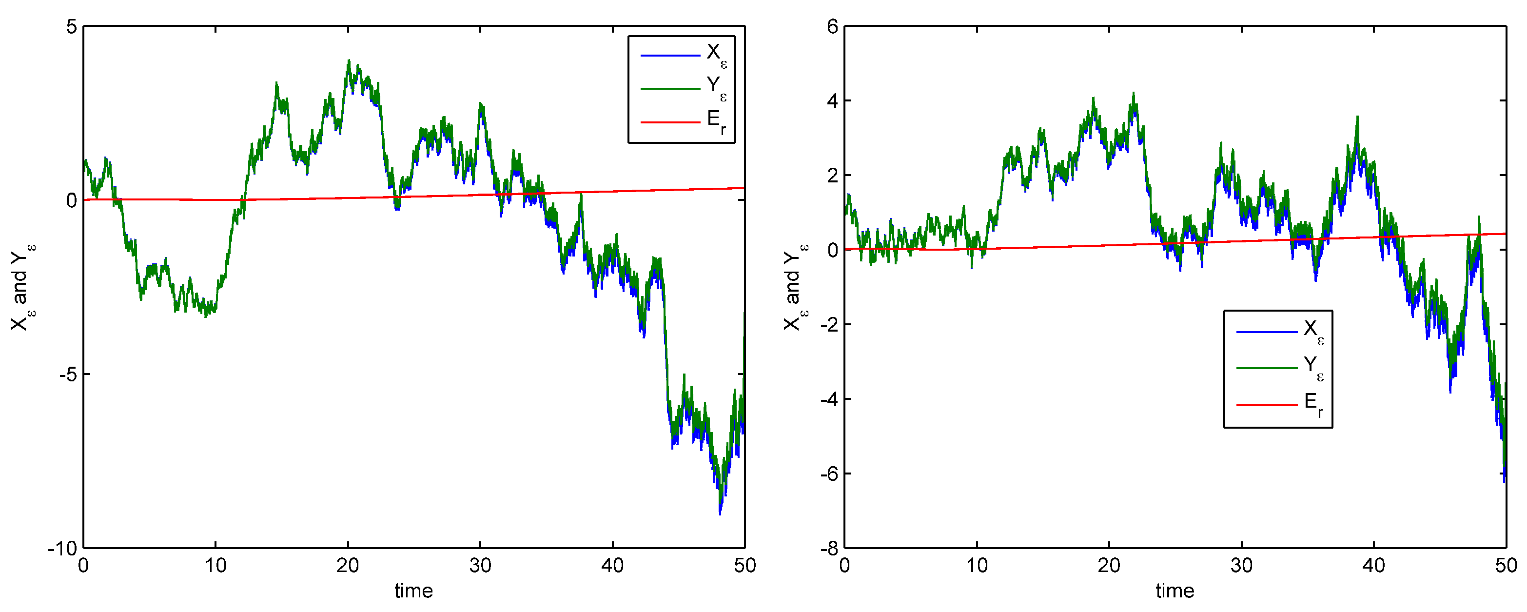
In this part, we establish the averaging principle for FSDE (1) in the sense of the pth moment. Firstly, taking the average of functions $b(·),\sigma (·)$, and $H(·)$ with respect to t, naming them $\overline{b}(·),\overline{\sigma }(·)$, and $\overline{H}(·)$, we have the following:

$$\begin{array}{ccc}\hfill \overline{b}\left(X\left(t\right)\right)& =& \underset{T_1\to \infty }{lim}{\displaystyle \frac{1}{T_1}}{\int }_0^{T_1}b(t,X\left(t\right))dt,\overline{\sigma }\left(X\left(t\right)\right)=\underset{T_1\to \infty }{lim}{\displaystyle \frac{1}{T_1}}{\int }_0^{T_1}\sigma (t,X\left(t\right))dt,\hfill \\ \hfill \overline{H}(X\left(t\right),x)& =& \underset{T_1\to \infty }{lim}{\displaystyle \frac{1}{T_1}}{\int }_0^{T_1}H(t,X\left(t\right),x)dt,\hfill \end{array}$$

with frozen slow components $X(·)$. Therefore, we can construct the following time-averaged equation

$$\begin{array}{ccc}\hfill {}^C\mathfrak{D}_0^{\alpha }Y\left(t\right)& =& ϵ\overline{b}\left(Y(t-)\right)+\sqrt{ϵ}\overline{\sigma }\left(Y(t-)\right){\displaystyle \frac{dB\left(t\right)}{dt}}+{\displaystyle \frac{\sqrt{ϵ}}{dt}}{\int }_{|x|<c}\overline{H}(Y(t-),x)\tilde{N}(dt,dx),\hfill \end{array}$$

(5)

with initial value $Y\left(0\right)=X\left(0\right)$, where $\overline{b}:{\mathbb{R}}^n\to {\mathbb{R}}^n$, $\overline{\sigma }:{\mathbb{R}}^n\to {\mathbb{R}}^n$, and $\overline{H}:{\mathbb{R}}^n\times {\mathbb{R}}^n\to {\mathbb{R}}^n$ are continuous functions. Here, $Y(·)$ is a stochastic process.

Remark 1 

(see [20], p. 193). If these three limits exist, the functions $\overline{b}(·),\overline{\sigma }(·)$, and $\overline{H}(·)$ also satisfy the linear growth condition and Lipschitz condition as functions $b(·),\sigma (·)$, and $H(·)$ with the same constant $C_1$. In addition, the limit ${lim}_{T_1\to \infty }{\displaystyle \frac{1}{T_1}}{\int }_0^{T_1}b({\xi }_t,X\left(t\right))dt=\overline{b}\left(X\left(t\right)\right)$ exists, for example, if ${\xi }_t$ is periodic or a sum of periodic functions.

Suppose functions $\overline{b}(·),\overline{\sigma }(·)$, and $\overline{H}(·)$ satisfy the following conditions:

$\left[A3\right]$: For any $t\ge 0$, $x\in {\mathbb{R}}^n$, there exist three positive bounded functions $K_1(·)$, $K_2(·)$, and $K_3(·)$ such that functions $\overline{b}(·),\overline{\sigma }(·)$, and $\overline{H}(·)$ satisfy

$$\begin{array}{c}\hfill {\displaystyle \frac{1}{t}}{\int }_0^t|b(s,X)-\overline{b}{\left(X\right)|}^{2}ds\le K_1{\left(t\right)(1+|X\left(t\right)|}^2),\\ \hfill {\displaystyle \frac{1}{t}}{\int }_0^t|\sigma (s,X)-\overline{\sigma }{\left(X\right)|}^{4}ds\le K_2{\left(t\right)(1+|X\left(t\right)|}^4),\\ \hfill {\displaystyle \frac{1}{t}}{\int }_0^t|{\int }_{|x|<c}{|H(s,Y(s-),x)-\overline{H}(Y(s-),x)|}^{2}v\left(dx\right){|}^{2}ds& \le & K_3{\left(t\right)(1+|X\left(t\right)|}^4),\hfill \end{array}$$

where ${lim}_{t\to \infty }{K}_i\left(t\right)=0,i=1,2,3$.

According to Lemma 2 and Remark 1, both FSDE (1) and averaged Equation (5) have unique solutions. Let $Y_{ϵ}$ be the unique solution of (5), $\kappa =max\{{\displaystyle \frac{p-1}{p}},{\displaystyle \frac{3}{4}}\},p\ge 2$. Now, we are ready to present the main result.

Theorem 1. 

If conditions $\left[A1\right],\left[A2\right]$, and $\left[A3\right]$ are satisfied, then there exists $L_1>0,{ϵ}_1\in [0,{ϵ}^{*}]$, and $\beta \in (0,1)$ such that for all $p\ge 2,ϵ\in (0,{ϵ}_1]$, $\alpha \in (\kappa ,1]$

$$\begin{array}{c}\hfill \underset{ϵ\to 0}{lim}E\left(\underset{t\in [0,L_1{ϵ}^{-\beta }]}{sup}{|X_{ϵ}\left(t\right)-Y_{ϵ}\left(t\right)|}^p\right)=0.\end{array}$$

Proof. 

For any $t\in [0,u]$, we have

$$\begin{array}{ccc}\hfill X_{ϵ}\left(t\right)-Y_{ϵ}\left(t\right)& =& {\displaystyle \frac{ϵ}{\Gamma \left(\alpha \right)}}{\int }_0^t[b(s,X_{ϵ}(s-))-\overline{b}\left(Y_{ϵ}(s-)\right)]{(t-s)}^{\alpha -1}ds\hfill \\ & & +{\displaystyle \frac{\sqrt{ϵ}}{\Gamma \left(\alpha \right)}}{\int }_0^t[\sigma (s,X_{ϵ}(s-))-\overline{\sigma }\left(Y_{ϵ}(s-)\right)]{(t-s)}^{\alpha -1}dB\left(s\right)\hfill \\ & & +{\displaystyle \frac{\sqrt{ϵ}}{\Gamma \left(\alpha \right)}}{\int }_0^t{(t-s)}^{\alpha -1}{\int }_{|x|<c}[H(s,X_{ϵ}(s-),x)-\overline{H}(Y_{ϵ}(s-),x)]\tilde{N}(ds,dx).\hfill \end{array}$$

From Lemma 3, we obtain $E\left({sup}_{t\in [0,T]}{|X\left(t\right)|}^p\right)<+\infty$ and $E\left({\int }_0^T{|X\left(s\right)|}^{p}ds\right)<+\infty$. Let $u<T$ be a variable. Thus, for any $p\ge 2$, using the inequality ${|a+b+c|}^p\le 3^{p-1}{(|a|}^p+{|b|}^p+{|c|}^p)$ and computing the expectation, we have

$$\begin{array}{ccc}\hfill & & E\left(\underset{t\in [0,u]}{sup}{|X_{ϵ}\left(t\right)-Y_{ϵ}\left(t\right)|}^p\right)\hfill \\ & \le & {\displaystyle \frac{3^{p-1}{ϵ}^p}{\Gamma {\left(\alpha \right)}^p}}E\left(\underset{t\in [0,u]}{sup}|{\int }_0^t[b(s,X_{ϵ}(s-))-\overline{b}\left(Y_{ϵ}(s-)\right)]{(t-s)}^{\alpha -1}ds{|}^p\right)\hfill \\ & & +{\displaystyle \frac{3^{p-1}{ϵ}^{\frac{p}{2}}}{\Gamma {\left(\alpha \right)}^p}}E\left(\underset{t\in [0,u]}{sup}|{\int }_0^t[\sigma (s,X_{ϵ}(s-))-\overline{\sigma }\left(Y_{ϵ}(s-)\right)]{(t-s)}^{\alpha -1}dB\left(s\right){|}^p\right)\hfill \\ & & +{\displaystyle \frac{3^{p-1}{ϵ}^{\frac{p}{2}}}{\Gamma {\left(\alpha \right)}^p}}E{\left(\underset{t\in [0,u]}{sup}{\int }_0^t{(t-s)}^{\alpha -1}{\int }_{|x|<c}[H(s,X_{ϵ}(s-),x)-\overline{H}(Y_{ϵ}(s-),x)]\tilde{N}(ds,dx)\right)}^p\hfill \\ & =:& I_1+I_2+I_3.\hfill \end{array}$$

(6)

Note that ${|a+b|}^p\le 2^{p-1}{|a|}^p+{|b|}^p$, so we obtain

$$\begin{array}{ccc}\hfill I_1& \le & {\displaystyle \frac{6^{p-1}{ϵ}^p}{\Gamma {\left(\alpha \right)}^p}}E\left(\underset{t\in [0,u]}{sup}|{\int }_0^t[b(s,X_{ϵ}(s-))-b(s,Y_{ϵ}(s-))]{(t-s)}^{\alpha -1}ds{|}^p\right)\hfill \\ & & +{\displaystyle \frac{6^{p-1}{ϵ}^p}{\Gamma {\left(\alpha \right)}^p}}E\left(\underset{t\in [0,u]}{sup}|{\int }_0^t[b(s,Y_{ϵ}(s-))-\overline{b}\left(Y_{ϵ}(s-)\right)]{(t-s)}^{\alpha -1}ds{|}^p\right)\hfill \\ & =:& I_{11}+I_{12}.\hfill \end{array}$$

Applying Hölder’s inequality and $\left[A1\right]$, we have

$$\begin{array}{ccc}\hfill I_{11}& \le & {\displaystyle \frac{6^{p-1}{ϵ}^p{u}^{p-1}}{\Gamma {\left(\alpha \right)}^p}}E\left(\underset{t\in [0,u]}{sup}{\int }_0^t|[b(s,X_{ϵ}(s-))-b(s,Y_{ϵ}(s-))]{(t-s)}^{\alpha -1}{|}^{p}ds\right)\hfill \\ & \le & {\displaystyle \frac{6^{p-1}{ϵ}^p{u}^{p-1}}{\Gamma {\left(\alpha \right)}^p}}{C}_1^p\underset{t\in [0,u]}{sup}{\int }_0^{u}E(|X_{ϵ}(s-)-Y_{ϵ}(s-){|}^p){(u-s)}^{p\alpha -p}ds\hfill \\ \hfill & \le & {\displaystyle \frac{6^{p-1}{ϵ}^p{u}^{p-1}}{\Gamma {\left(\alpha \right)}^p}}{C}_1^p{\int }_0^{u}E(\underset{\tau \in [0,s]}{sup}|X_{ϵ}\left(\tau \right)-Y_{ϵ}\left(\tau \right){|}^p){(u-s)}^{p\alpha -p}ds.\hfill \end{array}$$

(7)

Applying the Cauchy–Schwarz inequality and $\left[A3\right]$, we have

$$\begin{array}{ccc}\hfill I_{12}& \le & {\displaystyle \frac{6^{p-1}{ϵ}^p}{\Gamma {\left(\alpha \right)}^p}}{\left[\underset{t\in [0,u]}{sup}{\int }_0^t{(t-s)}^{2\alpha -2}dsE\left(\underset{t\in [0,u]}{sup}{\int }_0^t|b(s,Y_{ϵ}(s-))-\overline{b}\left(Y_{ϵ}(s-)\right){|}^{2}ds\right)\right]}^{{\displaystyle \frac{p}{2}}}\hfill \\ & \le & {\displaystyle \frac{6^{p-1}{ϵ}^p}{\Gamma {\left(\alpha \right)}^p}}{\left({\displaystyle \frac{u^{2\alpha -1}}{2\alpha -1}}\right)}^{{\displaystyle \frac{p}{2}}}E{\left(\underset{t\in [0,u]}{sup}\left[t·K_1\left(t\right)(1+|Y_{ϵ}\left(t\right){|}^2)\right]\right)}^{{\displaystyle \frac{p}{2}}}\hfill \\ & \le & {\displaystyle \frac{6^{p-1}{ϵ}^p{u}^{2p\alpha }}{\Gamma {\left(\alpha \right)}^p{(2\alpha -1)}^{\frac{p}{2}}}}{\left[\underset{t\in [0,u]}{sup}{K}_1\left(t\right)(1+E(\underset{t\in [0,u]}{sup}|Y_{ϵ}{\left(t\right)|}^2\left)\right)\right]}^{{\displaystyle \frac{p}{2}}}\hfill \\ \hfill & =& {\displaystyle \frac{6^{p-1}{ϵ}^p{u}^{2p\alpha }}{\Gamma {\left(\alpha \right)}^p{(2\alpha -1)}^{\frac{p}{2}}}}{{\rm Y}}_1,\hfill \end{array}$$

(8)

where ${{\rm Y}}_1=[{sup}_{t\in [0,u]}{K}_1\left(t\right)(1+E({sup}_{t\in [0,u]}|Y_{ϵ}{\left(t\right)|}^2{\left)\right)]}^{{\displaystyle \frac{p}{2}}}$ is a constant.

Note that ${|a+b|}^p\le 2^{p-1}{|a|}^p+{|b|}^p$, and applying Itô’s isometry, we have

$$\begin{array}{ccc}\hfill I_2& \le & {\displaystyle \frac{6^{p-1}{ϵ}^{\frac{p}{2}}}{\Gamma {\left(\alpha \right)}^p}}E\left(\underset{t\in [0,u]}{sup}|{\int }_0^t[\sigma (s,X_{ϵ}(s-))-\sigma (s,Y_{ϵ}(s-))]{(t-s)}^{\alpha -1}dB\left(s\right){|}^p\right)\hfill \\ & & +{\displaystyle \frac{6^{p-1}{ϵ}^{\frac{p}{2}}}{\Gamma {\left(\alpha \right)}^p}}E\left(\underset{t\in [0,u]}{sup}|{\int }_0^t[\sigma (s,Y_{ϵ}(s-))-\overline{\sigma }\left(Y_{ϵ}(s-)\right)]{(t-s)}^{\alpha -1}dB\left(s\right){|}^p\right)\hfill \\ & =& {\displaystyle \frac{6^{p-1}{ϵ}^{\frac{p}{2}}}{\Gamma {\left(\alpha \right)}^p}}E{\left(\underset{t\in [0,u]}{sup}{\int }_0^t|[\sigma (s,X_{ϵ}(s-))-\sigma (s,Y_{ϵ}(s-))]{(t-s)}^{\alpha -1}{|}^{2}ds\right)}^{{\displaystyle \frac{p}{2}}}\hfill \\ & & +{\displaystyle \frac{6^{p-1}{ϵ}^{\frac{p}{2}}}{\Gamma {\left(\alpha \right)}^p}}E{\left(\underset{t\in [0,u]}{sup}{\int }_0^t|[\sigma (s,Y_{ϵ}(s-))-\overline{\sigma }\left(Y_{ϵ}(s-)\right)]{(t-s)}^{\alpha -1}{|}^{2}ds\right)}^{{\displaystyle \frac{p}{2}}}\hfill \\ & =:& I_{21}+I_{22}.\hfill \end{array}$$

Applying $\left[A1\right]$, we have

$$\begin{array}{ccc}\hfill I_{21}& =& {\displaystyle \frac{6^{p-1}{ϵ}^{\frac{p}{2}}}{\Gamma {\left(\alpha \right)}^p}}E{\left(\underset{t\in [0,u]}{sup}{\int }_0^t|[\sigma (s,X_{ϵ}(s-))-\sigma (s,Y_{ϵ}(s-))]{(t-s)}^{\alpha -1}{|}^{2}ds\right)}^{{\displaystyle \frac{p}{2}}}\hfill \\ & \le & {\displaystyle \frac{6^{p-1}{ϵ}^{\frac{p}{2}}}{\Gamma {\left(\alpha \right)}^p}}{C}_1^{p}E{\left(\underset{t\in [0,u]}{sup}{\int }_0^t|[X_{ϵ}(s-)-Y_{ϵ}(s-)]{(t-s)}^{\alpha -1}{|}^{2}ds\right)}^{{\displaystyle \frac{p}{2}}}.\hfill \end{array}$$

(9)

Now, using Hölder’s inequality, we obtain

$$\begin{array}{ccc}\hfill I_{21}& \le & {\displaystyle \frac{6^{p-1}{ϵ}^{\frac{p}{2}}}{\Gamma {\left(\alpha \right)}^p}}{C}_1^{p}E{\left(\underset{t\in [0,u]}{sup}{\int }_0^t|[X_{ϵ}(s-)-Y_{ϵ}(s-)]{(t-s)}^{\alpha -1}{|}^{2}ds\right)}^{{\displaystyle \frac{p}{2}}}\hfill \\ & \le & {\displaystyle \frac{6^{p-1}{ϵ}^{\frac{p}{2}}}{\Gamma {\left(\alpha \right)}^p}}{C}_1^{p}E\left(\underset{t\in [0,u]}{sup}{\int }_0^t|[X_{ϵ}(s-)-Y_{ϵ}(s-)]{(t-s)}^{\alpha -1}{|}^{p}ds\right)\underset{t\in [0,u]}{sup}{\left({\int }_0^{t}1ds\right)}^{{\displaystyle \frac{p-2}{2}}}\hfill \\ \hfill & \le & {\displaystyle \frac{6^{p-1}{ϵ}^{\frac{p}{2}}}{\Gamma {\left(\alpha \right)}^p}}{u}^{{\displaystyle \frac{p-2}{2}}}{C}_1^p{\int }_0^{u}E(\underset{\tau \in [0,s]}{sup}|X_{ϵ}\left(\tau \right)-Y_{ϵ}\left(\tau \right){|}^p){(u-s)}^{p\alpha -p}ds.\hfill \end{array}$$

(10)

Next, using Hölder’s inequality and $\left[A3\right]$, one can show that

$$\begin{array}{ccc}\hfill I_{22}& \le & {\displaystyle \frac{6^{p-1}{ϵ}^{\frac{p}{2}}}{\Gamma {\left(\alpha \right)}^p}}E{\left(\underset{t\in [0,u]}{sup}{\int }_0^t|\sigma (s,Y_{ϵ}(s-))-\overline{\sigma }\left(Y_{ϵ}(s-)\right){|}^2{(t-s)}^{2\alpha -2}ds\right)}^{{\displaystyle \frac{p}{2}}}\hfill \\ & \le & {\displaystyle \frac{6^{p-1}{ϵ}^{\frac{p}{2}}}{\Gamma {\left(\alpha \right)}^p}}E\underset{t\in [0,u]}{sup}\left[{\left({\int }_0^t{(t-s)}^{4\alpha -4}ds\right)}^{{\displaystyle \frac{p}{4}}}{\left({\int }_0^t|\sigma (s,Y_{ϵ}(s-))-\overline{\sigma }\left(Y_{ϵ}(s-)\right){|}^{4}ds\right)}^{{\displaystyle \frac{p}{4}}}\right]\hfill \\ & \le & {\displaystyle \frac{6^{p-1}{ϵ}^{\frac{p}{2}}}{\Gamma {\left(\alpha \right)}^p}}{\left({\displaystyle \frac{u^{4\alpha -3}}{4\alpha -3}}\right)}^{{\displaystyle \frac{p}{4}}}{\left[\underset{t\in [0,u]}{sup}t·K_2\left(t\right)(1+E(\underset{t\in [0,u]}{sup}|Y_{ϵ}{\left(t\right)|}^4\left)\right)\right]}^{{\displaystyle \frac{p}{4}}}\hfill \\ \hfill & =& {\displaystyle \frac{6^{p-1}{ϵ}^{\frac{p}{2}}{u}^{\frac{p(2\alpha -1)}{2}}}{\Gamma {\left(\alpha \right)}^p{(4\alpha -3)}^{\frac{p}{4}}}}{{\rm Y}}_2,\hfill \end{array}$$

(11)

where ${{\rm Y}}_2={\left[{sup}_{t\in [0,u]}{K}_2\left(t\right)(1+E({sup}_{t\in [0,u]}|Y_{ϵ}{\left(t\right)|}^4\left)\right)\right]}^{{\displaystyle \frac{p}{4}}}$ is a constant.

In the sequel, for $I_3$, using Burkholder’s inequality, we have

$$\begin{array}{ccc}\hfill I_3& \le & {\displaystyle \frac{6^{p-1}{ϵ}^{\frac{p}{2}}}{\Gamma {\left(\alpha \right)}^p}}E{\left(\underset{t\in [0,u]}{sup}{\int }_0^t{(t-s)}^{\alpha -1}{\int }_{|x|<c}|H(s,X_{ϵ}(s-),x)-H(s,Y_{ϵ}(s-),x)|\tilde{N}(ds,dx)\right)}^p\hfill \\ & & +{\displaystyle \frac{6^{p-1}{ϵ}^{\frac{p}{2}}}{\Gamma {\left(\alpha \right)}^p}}E{\left(\underset{t\in [0,u]}{sup}{\int }_0^t{(t-s)}^{\alpha -1}{\int }_{|x|<c}|H(s,Y_{ϵ}(s-),x)-\overline{H}(Y_{ϵ}(s-),x)|\tilde{N}(ds,dx)\right)}^p\hfill \\ & \le & {\displaystyle \frac{6^{p-1}{ϵ}^{\frac{p}{2}}}{\Gamma {\left(\alpha \right)}^p}}E{\left(\underset{t\in [0,u]}{sup}{\int }_0^t{(t-s)}^{2\alpha -2}{\int }_{|x|<c}|H(s,X_{ϵ}(s-),x)-H(s,Y_{ϵ}(s-),x){|}^{2}v\left(dx\right)ds\right)}^{{\displaystyle \frac{p}{2}}}\hfill \\ & & +{\displaystyle \frac{6^{p-1}{ϵ}^{\frac{p}{2}}}{\Gamma {\left(\alpha \right)}^p}}E{\left(\underset{t\in [0,u]}{sup}{\int }_0^t{(t-s)}^{2\alpha -2}{\int }_{|x|<c}|H(s,Y_{ϵ}(s-),x)-\overline{H}(Y_{ϵ}(s-),x){|}^{2}v\left(dx\right)ds\right)}^{{\displaystyle \frac{p}{2}}}\hfill \\ & \le & I_{31}+I_{32}.\hfill \end{array}$$

Obviously, from $\left[A1\right]$, we obtain

$$\begin{array}{c}\hfill I_{31}\le {\displaystyle \frac{6^{p-1}{ϵ}^{\frac{p}{2}}}{\Gamma {\left(\alpha \right)}^p}}{C}_1^{p}E{\left(\underset{t\in [0,u]}{sup}{\int }_0^t|[X_{ϵ}(s-)-Y_{ϵ}(s-)]{(t-s)}^{\alpha -1}{|}^{2}ds\right)}^{{\displaystyle \frac{p}{2}}},\end{array}$$

which is the same as (9). Therefore, according to (10), we have

$$\begin{array}{ccc}\hfill I_{31}& \le & {\displaystyle \frac{6^{p-1}{ϵ}^{\frac{p}{2}}}{\Gamma {\left(\alpha \right)}^p}}{u}^{{\displaystyle \frac{p-2}{2}}}{C}_1^p{\int }_0^{u}E(\underset{\tau \in [0,s]}{sup}|X_{ϵ}\left(\tau \right)-Y_{ϵ}\left(\tau \right){|}^p){(u-s)}^{p\alpha -p}ds.\hfill \end{array}$$

(12)

From condition $\left[A3\right]$ and Hölder’s inequality, employing the same method as $I_{22}$, we have

$$\begin{array}{ccc}\hfill I_{32}& \le & {\displaystyle \frac{6^{p-1}{ϵ}^{\frac{p}{2}}}{\Gamma {\left(\alpha \right)}^p}}E\underset{t\in [0,u]}{sup}[{\left({\int }_0^t{(t-s)}^{4\alpha -4}ds\right)}^{{\displaystyle \frac{p}{4}}}\hfill \\ & & \times {\left({\int }_0^t|{\int }_{|x|<c}{|H(s,Y_{ϵ}(s-),x)-\overline{H}(Y_{ϵ}(s-),x)|}^{2}v\left(dx\right){|}^{2}ds\right)}^{{\displaystyle \frac{p}{4}}}]\hfill \\ \hfill & \le & {\displaystyle \frac{6^{p-1}{ϵ}^{\frac{p}{2}}{u}^{\frac{p(2\alpha -1)}{2}}}{\Gamma {\left(\alpha \right)}^p{(4\alpha -3)}^{\frac{p}{4}}}}{{\rm Y}}_3,\hfill \end{array}$$

(13)

where ${{\rm Y}}_3={\left[{sup}_{t\in [0,u]}{K}_3\left(t\right)(1+E({sup}_{t\in [0,u]}|Y_{ϵ}{\left(t\right)|}^4\left)\right)\right]}^{{\displaystyle \frac{p}{4}}}$ is a constant. Now, substitute (7), (8), and (10)–(13) into (6), we have

$$\begin{array}{ccc}& & E\left(\underset{t\in [0,u]}{sup}{|X_{ϵ}\left(t\right)-Y_{ϵ}\left(t\right)|}^p\right)\hfill \\ & \le & \left({\displaystyle \frac{6^{p-1}{ϵ}^p{u}^{2p\alpha }}{\Gamma {\left(\alpha \right)}^p{(2\alpha -1)}^{\frac{p}{2}}}}{{\rm Y}}_1+{\displaystyle \frac{6^{p-1}{ϵ}^{\frac{p}{2}}{u}^{\frac{p(2\alpha -1)}{2}}}{\Gamma {\left(\alpha \right)}^p{(4\alpha -3)}^{\frac{p}{4}}}}({{\rm Y}}_2+{{\rm Y}}_3)\right)\hfill \\ & & +{\displaystyle \frac{6^{p-1}{C}_1^p{ϵ}^{\frac{p}{2}}}{\Gamma {\left(\alpha \right)}^p}}({ϵ}^{{\displaystyle \frac{p}{2}}}{u}^{p-1}+2u^{{\displaystyle \frac{p-2}{2}}}){\int }_0^{u}E(\underset{\tau \in [0,s]}{sup}|X_{ϵ}\left(\tau \right)-Y_{ϵ}\left(\tau \right){|}^p){(u-s)}^{p\alpha -p}ds.\hfill \end{array}$$

Here, in order to make the integrals ${\int }_0^t{(t-s)}^{4\alpha -4}ds$ and ${\int }_0^t{(t-s)}^{p\alpha -p}ds$ solvable, we have to restrict $\alpha \in (\kappa ,1]$, $\kappa =max\{{\displaystyle \frac{p-1}{p}},{\displaystyle \frac{3}{4}}\}$. Thus, using the Gronwall–Bellman inequality (Lemma 1), we obtain

$$\begin{array}{c}\hfill E\left(\underset{t\in [0,u]}{sup}{|X_{ϵ}\left(t\right)-Y_{ϵ}\left(t\right)|}^p\right)\le \Phi \left(u\right)ϵ,\end{array}$$

(14)

where

$$\begin{array}{ccc}\hfill \Phi \left(u\right)& =& \left({\displaystyle \frac{6^{p-1}{ϵ}^{p-1}{u}^{2p\alpha }}{\Gamma {\left(\alpha \right)}^p{(2\alpha -1)}^{\frac{p}{2}}}}{{\rm Y}}_1+{\displaystyle \frac{6^{p-1}{ϵ}^{\frac{p}{2}-1}{u}^{\frac{p(2\alpha -1)}{2}}}{\Gamma {\left(\alpha \right)}^p{(4\alpha -3)}^{\frac{p}{4}}}}({{\rm Y}}_2+{{\rm Y}}_3)\right)\hfill \\ & & \times exp\left[{\displaystyle \frac{6^{p-1}{C}_1^p{ϵ}^{\frac{p}{2}}}{\Gamma {\left(\alpha \right)}^p}}({ϵ}^{{\displaystyle \frac{p}{2}}}{u}^{p-1}+2u^{{\displaystyle \frac{p-2}{2}}}){\displaystyle \frac{u^{p\alpha -p+1}}{p\alpha -p+1}}\right].\hfill \end{array}$$

This implies that we can select $\beta \in (0,1)$ and $L_1>0$, such that for all $t\in [0,L_1{ϵ}^{-\beta }]\subset [0,T]$, we have

$$\begin{array}{c}\hfill E\left(\underset{t\in [0,L_1{ϵ}^{-\beta }]}{sup}{|X_{ϵ}\left(t\right)-Y_{ϵ}\left(t\right)|}^p\right)\le {\Phi }_1\left(ϵ\right){ϵ}^{1-\beta },\end{array}$$

where

$$\begin{array}{ccc}\hfill {\Phi }_1\left(ϵ\right)& =& \left({\displaystyle \frac{6^{p-1}{L}_1^{2p\alpha }{ϵ}^{p+\beta -1-2p\alpha \beta }}{\Gamma {\left(\alpha \right)}^p{(2\alpha -1)}^{\frac{p}{2}}}}{{\rm Y}}_1+{\displaystyle \frac{6^{p-1}{L}_1^{\frac{p(2\alpha -1)}{2}}{ϵ}^{\frac{p+2\beta -2-p\beta (2\alpha -1)}{2}}}{\Gamma {\left(\alpha \right)}^p{(4\alpha -3)}^{\frac{p}{4}}}}({{\rm Y}}_2+{{\rm Y}}_3)\right)\hfill \\ & & \times exp\left[{\displaystyle \frac{6^{p-1}{C}_1^p{ϵ}^{\frac{p}{2}}}{\Gamma {\left(\alpha \right)}^p}}{\displaystyle \frac{L_1^{p\alpha -p+1}{ϵ}^{\beta (p-p\alpha -1)}}{p\alpha -p+1}}(L_1^{p-1}{ϵ}^{{\displaystyle \frac{p+2\beta -2p\beta }{2}}}+2L_1^{{\displaystyle \frac{p-2}{2}}}{ϵ}^{{\displaystyle \frac{\beta (2-p)}{2}}})\right],\hfill \end{array}$$

is a positive constant.

Note that ${\Phi }_1\left(ϵ\right)$ is an increasing continuous function with respect to variable $ϵ$, and ${inf}_{ϵ\ge 0}{\Phi }_1\left(ϵ\right){ϵ}^{1-\beta }=0$. Thus, we have ${lim}_{ϵ\to 0}{\Phi }_1\left(ϵ\right){ϵ}^{1-\beta }=0$ and ${lim}_{ϵ\to 0}{L}_1{ϵ}^{-\beta }\to +\infty$.

The proof is completed. □

Remark 2. 

According to Theorem 1 and Doob’s martingale inequality (see [21], Theorem 3.8, p. 14), for all $c>0$, we have

$$\begin{array}{c}\hfill P\left(\underset{t\in [0,L_1{ϵ}^{-\beta }]}{sup}|X_{ϵ}\left(t\right)-Y_{ϵ}\left(t\right)|>c\right)\le {\displaystyle \frac{E\left({sup}_{t\in [0,L_1{ϵ}^{-\beta }]}{|X_{ϵ}\left(t\right)-Y_{ϵ}\left(t\right)|}^p\right)}{c^p}}\le {\displaystyle \frac{{\Phi }_1\left(ϵ\right){ϵ}^{1-\beta }}{c^p}}.\end{array}$$

Note that ${lim}_{ϵ\to 0}{\Phi }_1\left(ϵ\right){ϵ}^{1-\beta }=0$ and ${lim}_{ϵ\to 0}{L}_1{ϵ}^{-\beta }\to +\infty$. This means that for all $c>0$, one has

$$\begin{array}{c}\hfill \underset{ϵ\to 0}{lim}P\left(\underset{t\in [0,L_1{ϵ}^{-\beta }]}{sup}|X_{ϵ}\left(t\right)-Y_{ϵ}\left(t\right)|\le c\right)=1.\end{array}$$

Hence, since $c>0$ is arbitrary, we obtain

$$\begin{array}{c}\hfill \underset{ϵ\to 0}{lim}P\left(\underset{t\in [0,L_1{ϵ}^{-\beta }]}{sup}|X_{ϵ}\left(t\right)-Y_{ϵ}\left(t\right)|=0\right)=1.\end{array}$$

This means that the original solution $Y_{ϵ}(·)$ can be approximated by the averaged solution $X_{ϵ}(·)$ in probability.

4. An Example

In this section, we present an example to demonstrate the procedure of the averaging principle for following Caputo type FSDEs with Lévy noise.

$$\begin{array}{c}\hfill \left\{\begin{array}{c}{}^C\mathfrak{D}_0^{\alpha }X\left(t\right)=2ϵ\left({\displaystyle \frac{cos(t+X(t\left)\right)}{e^t}}+1\right)+2\sqrt{ϵ}{\displaystyle \frac{dB\left(t\right)}{dt}}+{\displaystyle \frac{\sqrt{ϵ}}{dt}}{\int }_{|x|<c}{x}^{4}sin\left(X\left(t\right)\right){\displaystyle \frac{e^t+1}{e^t}}{v}_{\lambda }\left(dx\right),t\ge 0,\hfill \\ X\left(0\right)=1.\hfill \end{array}\right.\end{array}$$

(15)

Choose $\alpha \in (0.75,1],\lambda \in (0,2),\xi >0$, $p=2$, and a $\lambda$-stable Lévy jump measure $v_{\lambda }\left(dx\right)={\displaystyle \frac{\xi }{x^{1+\lambda }}}dx$. Set $b\left(X\left(t\right)\right)=2\left({\displaystyle \frac{cos(t+X_{ϵ}\left(t\right))}{e^t}}+1\right)$, $\sigma \left(X\right(t\left)\right)=2$, $H(X\left(t\right),x)=x^{4}sin\left(X_{ϵ}\left(t\right)\right){\displaystyle \frac{e^t+1}{e^t}}$, $t\ge 0$. Thus, with frozen slow component $X_{ϵ}$, one can compute

$$\begin{array}{ccc}\hfill \overline{b}\left(X\left(t\right)\right)& =& \underset{t\to \infty }{lim}{\displaystyle \frac{1}{t}}{\int }_0^{t}2\left({\displaystyle \frac{cos(t+X_{ϵ}\left(t\right))}{e^t}}+1\right)ds=2,\hfill \\ \hfill \overline{\sigma }\left(X\left(t\right)\right)& =& \underset{t\to \infty }{lim}{\displaystyle \frac{1}{t}}{\int }_0^t\sigma (t,X\left(t\right))ds=2,\hfill \end{array}$$

and

$$\begin{array}{ccc}& & \underset{t\to \infty }{lim}{\displaystyle \frac{1}{t}}{\int }_0^t{\int }_{|x|<c}{\displaystyle \frac{e^s+1}{e^s}}{\displaystyle \frac{\xi }{x^{1+\lambda }}}{x}^{4}sin\left(X_{ϵ}\left(t\right)\right)dxds\hfill \\ & =& \underset{t\to \infty }{lim}{\displaystyle \frac{1}{t}}{\int }_0^t{\displaystyle \frac{e^s+1}{e^s}}sin\left(X_{ϵ}\left(t\right)\right){\int }_{|x|<c}{\displaystyle \frac{\xi x^4}{x^{1+\lambda }}}dxds\hfill \\ & =& {\displaystyle \frac{\xi c^{4-\lambda }}{4-\lambda }}sin\left(X_{ϵ}\left(t\right)\right)\underset{t\to \infty }{lim}{\displaystyle \frac{1}{t}}{\int }_0^t{\displaystyle \frac{e^s+1}{e^s}}ds\hfill \\ & =& {\displaystyle \frac{\xi c^{4-\lambda }}{4-\lambda }}sin\left(X_{ϵ}\left(t\right)\right).\hfill \end{array}$$

Therefore, we obtain the following averaged equation

$$\begin{array}{c}\hfill \left\{\begin{array}{c}{}^C\mathfrak{D}_0^{\alpha }{Y}_{ϵ}\left(t\right)=2ϵ+{\displaystyle \frac{\sqrt{ϵ}\xi c^{4-\lambda }}{4-\lambda }}sin\left(Y_{ϵ}\left(t\right)\right)+\sqrt{ϵ}{\displaystyle \frac{dB\left(t\right)}{dt}},t\ge 0,\hfill \\ Y_{ϵ}\left(0\right)=1.\hfill \end{array}\right.\end{array}$$

(16)

Now, we check that condition $\left[A3\right]$ is satisfied. For function $b(·)$, we have

$$\begin{array}{ccc}\hfill {\displaystyle \frac{1}{t}}{\int }_0^t{|b(t,X_{ϵ})-\overline{b}\left(X_{ϵ}\right)|}^{2}dt& =& {\displaystyle \frac{2}{t}}{\int }_0^t\left|{\displaystyle \frac{{cos}^2(t+X_{ϵ})}{e^{2t}}}\right|dt\hfill \\ & \le & {\displaystyle \frac{2}{t}}{\int }_0^t{\displaystyle \frac{1}{e^{2t}}}dt\hfill \\ & =& {\displaystyle \frac{2}{t}}·{\displaystyle \frac{1}{2}}(1-e^{-2t})\hfill \\ & \le & {\displaystyle \frac{1-e^{-2t}}{t}}(1+|X_{ϵ}{|}^2).\hfill \end{array}$$

For function $H(·)$, we can calculate

$$\begin{array}{ccc}& & {\displaystyle \frac{1}{t}}{\int }_0^t|{\int }_{|x|<c}{|H(t,X,x)-\tilde{H}(X,x)|}^{2}v\left(dx\right){|}^{2}ds\hfill \\ & =& {\displaystyle \frac{1}{t}}{\int }_0^t|{\int }_{|x|<c}\xi e^{-2s}{|sin\left(X_{ϵ}\left(t\right)\right)|}^2{x}^{7-\lambda }dx{|}^{2}ds\hfill \\ & \le & {\displaystyle \frac{1-e^{-4t}}{4t}}{\displaystyle \frac{{\xi }^2{c}^{15-2\lambda }}{15-2\lambda }}(1+|X_{ϵ}\left(t\right){|}^2).\hfill \end{array}$$

Therefore, $\left[A3\right]$ is satisfied with $K_1\left(t\right)={\displaystyle \frac{1-e^{-2t}}{t}},K_3\left(t\right)={\displaystyle \frac{1-e^{-4t}}{4t}}{\displaystyle \frac{{\xi }^2{c}^{15-2\lambda }}{15-2\lambda }},t\ge 0$. Next, let $E_r={|X_{ϵ}-Y_{ϵ}|}^2$ be the approximation error. With the help of MATLAB software, we show the averaged solution of (16) can converge to the original solution of (15) and their approximation error $E_r$ on the interval $[0,50]$; see Figure 1.

5. Conclusions

By developing the approach in [10], sufficient conditions were established to guarantee an averaging principle for Caputo type FSDEs with non-Gaussian Lévy noise in the sense of the pth moment. Different from previous work [15], the method presented in this paper can successfully deal with the singular integral kernel caused by fractional integration, and we proved the desired averaging principle for FSDEs in the sense of the pth moment. The explored technique can be used to deal with other type of FSDEs with non-Gaussian Lévy noise.

References

1. Xu, W.; Xu, W.; Zhang, S. The averaging principle for stochastic differential equations with Caputo fractional derivative. Appl. Math. Lett. 2019, 93, 79–84. [Google Scholar] [CrossRef]
2. Guo, Z.; Hu, J.; Yuan, C. Averaging principle for a type of Caputo fractional stochastic differential equations. Chaos 2021, 31, 053123. [Google Scholar] [CrossRef] [PubMed]
3. Gao, P. Averaging principle for multiscale stochastic reaction-diffusion-advection equations. Math. Methods Appl. Sci. 2019, 42, 1122–1150. [Google Scholar] [CrossRef]
4. Luo, D.; Zhu, Q.; Zhang, Z. An averaging principle for stochastic fractional differential equations with time-delays. Appl. Math. Lett. 2020, 105, 106290. [Google Scholar] [CrossRef]
5. Ahmed, H.M.; Zhu, Q. The averaging principle of Hilfer fractional stochastic delay differential equations with Poisson jumps. Appl. Math. Lett. 2021, 112, 106755. [Google Scholar] [CrossRef]
6. Xu, W.; Xu, W. An effective averaging theory for fractional neutral stochastic equations of order 0<α<1 with Poisson jumps. Appl. Math. Lett. 2020, 106, 106344. [Google Scholar]
7. Xu, W.; Xu, W.; Lu, K. An averaging principle for stochastic differential equations of fractional order 0<α<1. Fract. Calc. Appl. Anal. 2020, 23, 908–919. [Google Scholar]
8. Li, M.; Wang, J. The existence and averaging principle for Caputo fractional stochastic delay differential systems. Fract. Calc. Appl. Anal. 2023, 26, 893–912. [Google Scholar] [CrossRef]
9. Wang, Q.; Han, Z.; Zhang, X.; Yang, Y. Dynamics of the delay-coupled bubble system combined with the stochastic term. Chaos Solitons Fractals 2021, 148, 111053. [Google Scholar] [CrossRef]
10. Xiao, G.; Fečkan, M.; Wang, J. On the averaging principle for stochastic differential equations involving Caputo fractional derivative. Chaos 2022, 32, 101105. [Google Scholar] [CrossRef] [PubMed]
11. Zhu, Q. Stability of stochastic differential equations with Lévy noise. In Proceedings of the 33rd Chinese Control Conference, Nanjing, China, 28–30 July 2014; pp. 5211–5216. [Google Scholar]
12. Xu, Y.; Duan, J.; Xu, W. An averaging principle for stochastic dynamical systems with Lévy noise. Physica D 2011, 240, 1395–1401. [Google Scholar] [CrossRef]
13. Shen, G.; Xu, W.; Wu, J. An averaging principle for stochastic differential delay equations driven by time-changed Lévy noise. Acta Math. Sci. 2022, 42, 540–550. [Google Scholar] [CrossRef]
14. Shen, G.; Xiao, R.; Yin, X. Averaging principle and stability of hybrid stochastic fractional differential equations driven by Lévy noise. Int. J. Syst. Sci. 2020, 51, 2115–2133. [Google Scholar] [CrossRef]
15. Xu, W.; Duan, J.; Xu, W. An averaging principle for fractional stochastic differential equations with Lévy noise. Chaos 2020, 30, 083126. [Google Scholar] [CrossRef] [PubMed]
16. Guo, Z.; Fu, H.; Wang, W. An averaging principle for caputo fractional stochastic differential equations with compensated Poisson random measure. J. Partial. Differ. Equ. 2022, 35, 1–10. [Google Scholar]
17. Kilbas, A.A.; Srivastava, H.M.; Trujillo, J.J. Theory and Applications of Fractional Differential Equations; Elsevier: Amsterdam, The Netherlands, 2006. [Google Scholar]
18. Ye, H.; Gao, J.; Ding, Y. A generalized Gronwall inequality and its application to a fractional differential equation. J. Math. Anal. Appl. 2007, 328, 1075–1081. [Google Scholar] [CrossRef]
19. Umamaheswari, P.; Balachandran, K.; Annapoorani, N. Existence and stability results for Caputo fractional stochastic differential equations with Lévy noise. Filomat 2020, 34, 1739–1751. [Google Scholar] [CrossRef]
20. Freidlin, M.I.; Wentzell, A.D. Random Perturbations of Dynamical Systems, 3rd ed.; Springer: Berlin/Heidelberg, Germany, 2012. [Google Scholar]
21. Mao, X. Stochastic Differential Equations and Application, 2nd ed.; Horwood Publishing Limited: Chichester, UK, 2007. [Google Scholar]
Figure 1. Comparison of X ϵ and Y ϵ with α = 0.8 , ϵ = 0.005 and α = 0.9 , ϵ = 0.02 on the time interval [ 0 , 50 ] .
Fractalfract 08 00595 g001
Disclaimer/Publisher’s Note: The statements, opinions and data contained in all publications are solely those of the individual author(s) and contributor(s) and not of MDPI and/or the editor(s). MDPI and/or the editor(s) disclaim responsibility for any injury to people or property resulting from any ideas, methods, instructions or products referred to in the content.