Formation of Optical Fractals by Chaotic Solitons in Coupled Nonlinear Helmholtz Equations

Abstract

In the present research work, we construct and examine the self-similarity of optical solitons by employing the Riccati Modified Extended Simple Equation Method (RMESEM) within the framework of non-integrable Coupled Nonlinear Helmholtz Equations (CNHEs). This system models the transmission of optical solitons and coupled wave packets in nonlinear optical fibers and describes transverse effects in nonlinear fiber optics. Initially, a complex transformation is used to convert the model into a single Nonlinear Ordinary Differential Equation (NODE), from which hyperbolic, exponential, rational, trigonometric, and rational hyperbolic solutions are produced. In order to better understand the physical dynamics, we offer several 3D, contour, and 2D illustrations for the independent selections of physical parameter values. These illustrations highlight the graphic behaviour of some optical solitons and demonstrate that, under certain constraint conditions, acquired optical solitons lose their stability when they approach an axis and display periodic-axial perturbations, which lead to the generation of optical fractals. As a framework, the generated optical solitons have several useful applications in the field of telecommunications. Furthermore, our suggested RMESEM demonstrates its use by broadening the spectrum of optical soliton solutions, offering important insights into the dynamics of the CNHEs, and suggesting possible applications in the management of nonlinear models.

1. Introduction

Nonlinear Differential Equations (NDEs) particularly Nonlinear Partial Differential Equations (NPDEs) have important applications in various fields of science such as stochastic Schrödinger equations in spontaneous emissions or thermal fluctuations [1], nonlinear Maccari’s systems in plasma physics and hydrodynamics [2], the Navier Stokes equation in fluid [3], Higgs equations in particle physics [4], the Duffing equations in oscillatory motions [5], and Kairat equations in optics [6]. Several numerical and analytical approaches have been developed by researchers to explore the underpinning nature of NPDEs. However, there are several challenges associated with solving NPDEs. These obstacles include the potential for numerous or no solutions, sensitivity to the initial conditions, nonlinearity-related complexity, and difficulty in precisely determining the solution. By offering important insights into the dynamics of nonlinear models, exact solutions of NPDEs in contrast with numerical solutions, particularly the calculation of travelling wave and soliton solutions, are crucial to the study of soliton theory. Numerous useful approaches have been established to obtain soliton solutions for understanding the physical behaviour of these nonlinear models, which aid engineers and other experts as well as provide knowledge about physical issues and their applications. Giving precise soliton solutions for NPDEs with symbolic computer tools like Matlab, Maple, Mathematica, and others that simplify intricate algebraic calculations has garnered more attention in recent years. The literature has several analytical techniques for locating novel soliton solutions, including the Khater method [7], the Sine–Gordon method [8], the Riccati–Bernoulli Sub-ODE method [9], the $(G^{\prime }/G)$-expansion method [10,11,12,13], the exp-function method [14], the Sardar sub-equation method [15], the Kudryashov method [16], the Poincaré-Lighthill-Kuo method [17], Hirota’s bilinear method [18], the extended direct algebraic method [19,20], and the modified simple equation method [21,22], among others. It is also essential to recognize that these methods may have drawbacks and limits (like the seven common errors) [23,24], even though these approaches greatly advance our comprehension of soliton dynamics and help us to relate them to the theories that explain phenomena. Additionally, many of these methods depend on the Riccati equation [25]. Since the Riccati equation has solitary solutions, such techniques are useful in the study of soliton phenomena in nonlinear models [26].

Contemporary advances in soliton theory have led to fascinating new fields of study in the subject of mathematics, particularly, fractal soliton theory, which examines the intricate connection between solitons and fractals [27,28,29]. A stable, confined wave packet exhibiting both solitonic and fractal geometry is called a fractal soliton. Fractal solitons are solitons with uneven boundaries that exhibit self-replication and intricate geometrical structures at various scales while maintaining a steady speed. The relationship between soliton dynamics and fractal geometry provides fresh insights into nonlinear phenomena in physics, engineering, as well as biological frameworks [30,31,32]. Therefore, the theory of fractal solitons has many real-world applications in several domains. For instance, fractal solitons are useful in chaos theory because of their special characteristics, which aids in comprehending the dynamics and resilience of chaotic systems. The research on fractal solitons has become a hot issue in modern mathematics, and as it continues to develop, it is anticipated to encourage creative approaches and solutions in both practical and theoretical mathematics.

In this study, a robust and efficient analytical technique namely RMESEM is applied to address CNHEs in order to discover and explore a unique array of optical soliton solutions for them. The RMESEM is one of the most significant simple and effective algebraic procedures among the previously discussed analytical methods for generating soliton solutions to NPDEs. The strategic RMESEM reduces the problem to a set of nonlinear algebraic equations by transforming NPDEs into NODEs using a wave transformation and then assuming a series form solution. Novel families of soliton solutions, including exponential, rational, hyperbolic, and trigonometric functions, are obtained after solving the resulting system by employing the Maple tool. A single, sustainable wave packet that travels across a medium without changing its speed is known as a soliton. Since soliton solutions for NPDEs provide greater depth and granularity than traditional solutions, they continue to be important from an academic standpoint. They are useful because they maintain their innate durability and endurance in a variety of scientific and technical domains.

The aim of this research is to examine optical soliton propagation in CNHEs, which is a crucial Schrödinger-class model for altering the phase and amplitude modulation of continuous waves, as well as for modeling the growing miniaturization of plasmonics and photonic devices. Physically, this system models the transmission of optical solitons and coupled wave packets in nonlinear optical fibers and describes transverse effects in nonlinear fiber optics [33]. This model is expressed as the given coupled NPDEs [34]:

$$\begin{array}{cc}\hfill & i{w}_t+\phi w_{tt}+{\displaystyle \frac{1}{2}}{w}_{xx}+{\kappa }_1\left|w^2\right|w+{\kappa }_2\left|z^2\right|w=0,\hfill \\ \hfill & i{z}_t+\phi z_{tt}+{\displaystyle \frac{1}{2}}{z}_{xx}+{\kappa }_1\left|w^2\right|z+{\kappa }_2\left|z^2\right|z=0,\hfill \end{array}$$

(1)

where $i=\sqrt{-1}$, $w=w(x,t)$, and $z=z(x,t)$ represent envelope fields, while the subscripts x and t indicate the transverse and longitudinal coordinates correspondingly. In Equation (1), the second terms $\phi w_{tt}$ and $\phi z_{tt}$ are corresponded to Helmholtz nonparaxiality, while the coefficient $\phi (>$$0)$ symbolizes the parameter of nonparaxial, and ${\kappa }_1$ and ${\kappa }_2$ are the coefficients of nonlinearity that might potentially be included into the model itself with slight modifications. Moreover, the coefficients ${\kappa }_1$ and ${\kappa }_2$ are kept in (1) to deal with different nonlinearities namely, focusing nonlinearity $({\kappa }_1,{\kappa }_2>0)$ and mixed (focusing–defocusing) nonlinearity $({\kappa }_1>0,{\kappa }_2<0$ or ${\kappa }_1<0,{\kappa }_2>0)$ and defocusing nonlinearity $({\kappa }_1,{\kappa }_2<0)$. This model leads (1) to a Helmholtz–Manakov system for ${\kappa }_1={\kappa }_2=\pm 1$.

Many other scholars have addressed the targeted CNHEs using various analytical and numerical approaches before this research project. For instance, Tamilselvan et al. employed the ansatz approach to derive a class of elliptic wave solutions of CNHEs in terms of the Jacobi elliptic functions that characterize non-paraxial ultra-broad beam propagation in nonlinear Kerr-like media. They also examined the limiting forms of these solutions, particularly hyperbolic solutions [35]. Singh et al. employed the exp$(-\Phi (\epsilon \left)\right)$-expansion technique in [36] to derive travelling wave solutions for non-integrable CNHEs that were organised as trigonometric, rational, and hyperbolic functions. Similarly, Alsaud et al. used the generalized (G′/G)-expansion approach to obtain certain optical solitons for CNHEs and then provided an analysis of modulation instability based on the obtained optical solitons [34]. Finally, in the framework of a cubic CNHE, Saha et al. in [37] examined the presence and stability characteristics of anti-dark and chirped grey solitary waves.

It is obvious from the literature that scholars have previously investigated solitonic phenomena in CNHEs, but no study has been conducted to examine and evaluate the formation of optical fractals resulting from chaotic perturbations in solitons within the context of the aimed model. This observation points to a substantial gap in the corpus of existing research. Our research, which employs the suggested RMESEM technique, closes this gap by offering an in-depth and novel analysis of the model’s fractal solitonic phenomena. To do this, we generate and analyze novel optical solitons in the form of exponential, hyperbolic, trigonometric, and rational solutions for the non-integrable CNHEs using the RMESEM. We also provide several 3D, 2D, and contour visuals of acquired optical solitons to illustrate their dynamical behaviours, which reveal that, when acquired optical solitons approach an axis, they become unsustainable under specific constraint circumstances and exhibit periodic-axial disturbances, resulting in the formation of optical fractals. There may be several practical uses for the produced optical solitons in the telecom industry.

The rest of the paperwork is arranged as follows: Section 2 provides an explanation of the RMESEM’s analytical procedures. Section 3 addresses the CNHEs in order to produce new optical soliton solutions. Section 4 provides visual representations of the perturbed behaviour of the produced optical solitons. Section 5 provides the conclusion, and the Appendix A contains the details about wave functions.

2. The Methodology of RMESEM

Numerous analytical techniques have been developed in the literature to investigate soliton occurrences in nonlinear models [21,22,23,24,25,26,27,28,29,30,31,32,33,34,35]. However, in this study, we use the RMESEM to construct and examine optical soliton solutions for targeted CNHEs. This section outlines the efficient RMESEM’s operational mechanism. Suppose the NPDE of the form [6]:

$$A(\mathfrak{z},{\mathfrak{z}}_t,{\mathfrak{z}}_{t_1},{\mathfrak{z}}_{t_2},\mathfrak{z}{\mathfrak{z}}_{t_1},\dots )=0,$$

(2)

where $\mathfrak{z}=\mathfrak{z}(t,t_1,t_2,t_3,\dots ,t_r)$.

To solve (2), the following steps are performed:

1. Initially, we execute the variable-form complex transformation $\mathfrak{z}(t,t_1,t_2,t_3,\dots ,t_r)=\mathfrak{S}\left(\chi \right)$, which can be defined in multiple ways. Using this transformation, the following NODE is obtained from (2):

$$B(\mathfrak{S},{\mathfrak{S}}^{\prime }\mathfrak{S},{\mathfrak{S}}^{\prime },\dots )=0,$$

(3)

where ${\mathfrak{S}}^{\prime }={\displaystyle \frac{d\mathfrak{S}}{d\chi }}$. Occasionally, we integrate (3) to coerce the NODE to adhere to the homogenous balancing criterion.

2. Next, the ensuing finite series-based solution for the NODE in (3) is proposed using the solution of the extended Riccati–NODE:

$$\mathfrak{S}\left(\chi \right)=\sum _{j=0}^P{c}_j{\left({\displaystyle \frac{Q^{\prime }\left(\chi \right)}{Q\left(\chi \right)}}\right)}^j+\sum _{j=0}^{P-1}{d}_j{\left({\displaystyle \frac{Q^{\prime }\left(\chi \right)}{Q\left(\chi \right)}}\right)}^j·\left({\displaystyle \frac{1}{Q\left(\chi \right)}}\right).$$

(4)

Here, $Q\left(\chi \right)$ denotes the solution to the resulting extended Riccati–NODE, and the variables $c_j(j=0,\dots ,P)$ and $d_j(j=0,\dots ,P-1)$ represent the unknown constants that need to be discovered.

$$Q^{\prime }\left(\chi \right)=\rho +\varrho Q\left(\chi \right)+\sigma {\left(Q\left(\chi \right)\right)}^2,$$

(5)

where $\rho ,\varrho$ and $\sigma$ are constants.

3. By homogeneously balancing the largest nonlinear term and the highest-order derivative in Equation (3), we can accomplish the positive integer P required in Equation (4).

4. Then, when (4) is incorporated into (3) or in the equation that results from the integration of (3), all of the terms with the same powers of $Q\left(\chi \right)$ are collected, which results in the formation of an equation in terms of $Q\left(\chi \right)$. An algebraic system of equations describing the variables $c_j(j=0,...,P)$ and $d_j(j=0,...,P-1)$ with additional associated parameters may be obtained by setting the coefficients in the resultant equation to zero.

5. The resultant system of nonlinear algebraic equations is analytically solved using Maple.

6. Finally, we compute and insert the unknown values along with $Q\left(\chi \right)$ (the Equation (5)’s solution) in Equation (4) to obtain analytical soliton solutions for (2). We may obtain multiple clusters of soliton solutions by using the general solution of (5). These clusters are shown as follows: (see

Table 1. The particular solutions $Q\left(\chi \right)$ of the Riccati equation in (5) and the formation of $\left({\displaystyle \frac{Q^{\prime }\left(\chi \right)}{Q\left(\chi \right)}}\right)$, where $z_1,z_2\in \mathrm{R}$, $\upsilon ={\varrho }^2-4\sigma \rho$, and $\theta =cosh\left({\displaystyle \frac{1}{4}}\sqrt{\upsilon }\chi \right)sinh\left({\displaystyle \frac{1}{4}}\sqrt{\upsilon }\chi \right)$.

S. No.	Cluster	Constraint(s)	$\mathit{Q}\left(\mathit{\chi }\right)$	$\left(\frac{{\mathit{Q}}^{\prime }\left(\mathit{\chi }\right)}{\mathit{Q}\left(\mathit{\chi }\right)}\right)$
1	Trigonometric Solutions	$\upsilon <0,\sigma \ne 0$
			$-{\displaystyle \frac{\varrho }{2\sigma }}+{\displaystyle \frac{\sqrt{-\upsilon }tan\left(\frac{1}{2}\sqrt{-\upsilon }\chi \right)}{2\sigma }}$,	$-{\displaystyle \frac{1}{2}}{\displaystyle \frac{\upsilon \left(1+{\left(tan\left(\frac{1}{2}\sqrt{-\upsilon }\chi \right)\right)}^2\right)}{-\varrho +\sqrt{-\upsilon }tan\left(\frac{1}{2}\sqrt{-\upsilon }\chi \right)}}$,
			$-{\displaystyle \frac{\varrho }{2\sigma }}-{\displaystyle \frac{\sqrt{-\upsilon }cot\left(\frac{1}{2}\sqrt{-\upsilon }\chi \right)}{2\sigma }}$,	${\displaystyle \frac{1}{2}}{\displaystyle \frac{\left(1+{\left(cot\left(\frac{1}{2}\sqrt{-\upsilon }\chi \right)\right)}^2\right)\upsilon }{\varrho +\sqrt{-\upsilon }cot\left(\frac{1}{2}\sqrt{-\upsilon }\chi \right)}}$,
			$-{\displaystyle \frac{\varrho }{2\sigma }}+{\displaystyle \frac{\sqrt{-\upsilon }\left(tan\left(\sqrt{-\upsilon }\chi \right)+\left(sec\left(\sqrt{-\upsilon }\chi \right)\right)\right)}{2\sigma }}$,	${\displaystyle \frac{-\upsilon \left(1+sin\left(\sqrt{-\upsilon }\chi \right)\right)sec\left(\sqrt{-\upsilon }\chi \right)}{-\varrho cos\left(\sqrt{-\upsilon }\chi \right)+\sqrt{-\upsilon }sin\left(\sqrt{-\upsilon }\chi \right)+\sqrt{-\upsilon }}}$,
			$-{\displaystyle \frac{\varrho }{2\sigma }}+{\displaystyle \frac{\sqrt{-\upsilon }\left(tan\left(\sqrt{-\upsilon }\chi \right)-\left(sec\left(\sqrt{-\upsilon }\chi \right)\right)\right)}{2\sigma }}$.	${\displaystyle \frac{\upsilon \left(sin\left(\sqrt{-\upsilon }\chi \right)-1\right)sec\left(\sqrt{-\upsilon }\chi \right)}{-\varrho cos\left(\sqrt{-\upsilon }\chi \right)+\sqrt{-\upsilon }sin\left(\sqrt{-\upsilon }\chi \right)-\sqrt{-\upsilon }}}$.
2	Hyperbolic Solutions	$\upsilon >0,\sigma \ne 0$
			$-{\displaystyle \frac{\varrho }{2\sigma }}-{\displaystyle \frac{\sqrt{\upsilon }tanh\left(\frac{1}{2}\sqrt{\upsilon }\chi \right)}{2\sigma }}$,	$-{\displaystyle \frac{1}{2}}{\displaystyle \frac{\left(-1+{\left(tanh\left(\frac{1}{2}\sqrt{\upsilon }\chi \right)\right)}^2\right)\upsilon }{\varrho +\sqrt{\upsilon }tanh\left(\frac{1}{2}\sqrt{\upsilon }\chi \right)}}$,
			$-{\displaystyle \frac{\varrho }{2\sigma }}-{\displaystyle \frac{\sqrt{\upsilon }\left(tanh\left(\sqrt{\upsilon }\chi \right)+i\left(\mathrm{sech}\left(\sqrt{\upsilon }\chi \right)\right)\right)}{2\sigma }}$,	$-{\displaystyle \frac{\upsilon \left(-1+isinh\left(\sqrt{\upsilon }\chi \right)\right)}{cosh\left(\sqrt{\upsilon }\chi \right)\left(\varrho cosh\left(\sqrt{\upsilon }\chi \right)+\sqrt{\upsilon }sinh\left(\sqrt{\upsilon }\chi \right)+i\sqrt{\upsilon }\right)}}$,
			$-{\displaystyle \frac{\varrho }{2\sigma }}-{\displaystyle \frac{\sqrt{\upsilon }\left(tanh\left(\sqrt{\upsilon }\chi \right)-i\left(\mathrm{sech}\left(\sqrt{\upsilon }\chi \right)\right)\right)}{2\sigma }}$,	$-{\displaystyle \frac{\upsilon \left(1+isinh\left(\sqrt{\upsilon }\chi \right)\right)}{cosh\left(\sqrt{\upsilon }\chi \right)\left(-\varrho cosh\left(\sqrt{\upsilon }\chi \right)-\sqrt{\upsilon }sinh\left(\sqrt{\upsilon }\chi \right)+i\sqrt{\upsilon }\right)}},$
			$-{\displaystyle \frac{\varrho }{2\sigma }}-{\displaystyle \frac{\sqrt{\upsilon }\left(coth\left(\sqrt{\upsilon }\chi \right)+\left(\mathrm{csch}\left(\sqrt{\upsilon }\chi \right)\right)\right)}{2\sigma }}$.	$-{\displaystyle \frac{1}{4}}{\displaystyle \frac{\upsilon \left(2{\left(cosh\left(\frac{1}{4}\sqrt{\upsilon }\chi \right)\right)}^2-1\right)}{\theta \left(-2\varrho \theta +\sqrt{\upsilon }\right)}}.$
3	Rational Solutions
		$\upsilon =0$	$-2{\displaystyle \frac{\rho \left(\varrho \chi +2\right)}{{\varrho }^2\chi }}$,	$-2{\displaystyle \frac{1}{\chi \left(\varrho \chi +2\right)}}$,
		$\upsilon =0$, & $\varrho =\sigma =0$	$\chi \rho$,	${\displaystyle \frac{1}{\chi }}$,
		$\upsilon =0$, & $\varrho =\rho =0$	$-{\displaystyle \frac{1}{\chi \sigma }}$.	$-{\displaystyle \frac{1}{\chi }}$.
4	Exponential Solutions
		$\sigma =0$, & $\varrho =\mu$, $\rho =b\mu$	$e^{\mu \chi }-b$,	${\displaystyle \frac{\mu {\mathrm{e}}^{\mu \chi }}{{\mathrm{e}}^{\mu \chi }-b}}$,
		$\rho =0$, & $\varrho =\mu$, $\sigma =b\mu$	${\displaystyle \frac{e^{\mu \chi }}{1-b{e}^{\mu \chi }}}$.	$-{\displaystyle \frac{\mu }{-1+b{\mathrm{e}}^{\mu \chi }}}$.
5	Rational-Hyperbolic Solutions
		$\rho =0$, & $\varrho \ne 0$, $\sigma \ne 0$	$-{\displaystyle \frac{\varrho z_1}{\sigma \left(cosh\left(\varrho \chi \right)-sinh\left(\varrho \chi \right)+z_2\right)}}$,	${\displaystyle \frac{\varrho \left(sinh\left(\varrho \chi \right)-cosh\left(\varrho \chi \right)\right)}{-cosh\left(\varrho \chi \right)+sinh\left(\varrho \chi \right)-z_2}}$,
			$-{\displaystyle \frac{\varrho \left(cosh\left(\varrho \chi \right)+sinh\left(\varrho \chi \right)\right)}{\sigma \left(cosh\left(\varrho \chi \right)+sinh\left(\varrho \chi \right)+z_2\right)}}$.	${\displaystyle \frac{\varrho z_2}{cosh\left(\varrho \chi \right)+sinh\left(\varrho \chi \right)+z_2}}$.

).

3. Establishing Optical Soliton Solutions for CNHEs

In this study, we present optical soliton solutions for Equation (1) by utilizing the suggested RMESEM. We start with the complex wave transformation that is as follows:

$$\begin{array}{cc}\hfill w(x,t)=e^{\vartheta i}W\left(\chi \right),& z(x,t)=e^{\vartheta i}Z\left(\chi \right),\hfill \\ \hfill \chi =(k_{3}x-k_3{k}_{4}t),& \vartheta =(-k_{1}x+k_{2}t+\nu ).\hfill \end{array}$$

(6)

After substituting (6) in (1) and separating the imaginary and real parts, we obtain

$$\begin{array}{cc}\hfill & ({-k_3}^2-2\phi {k_3}^2{k_4}^2)W^{″}+({k_1}^2+2k_2+2\phi {k_2}^2)W+(-2{\kappa }_1{W}^3-2{\kappa }_{2}W{Z}^2)=0,\hfill \\ \hfill & (2k_1{k}_3+2k_3{k}_4+4\phi k_2{k}_3{k}_4)W^{\prime }=0,\hfill \end{array}$$

(7)

from Equation (1)’s real part, whereas its imaginary part produces

$$\begin{array}{cc}\hfill & ({-k_3}^2-2\phi {k_3}^2{k_4}^2)Z^{″}+({k_1}^2+2k_2+2\phi {k_2}^2)Z+(-2{\kappa }_1{W}^{2}Z-2{\kappa }_2{Z}^3)=0,\hfill \\ \hfill & (2k_1{k}_3+2k_3{k}_4+4\phi k_2{k}_3{k}_4)Z^{\prime }=0.\hfill \end{array}$$

(8)

When (8) undergoes transformation via $Z=\beta W$, we mitigate the entire system to a single NODE whenever $\beta$ is set to 1; alternatively, the system fails to be solved using the RMESEM. The resultant NODE is given as

$${\Pi }_{1}W+{\Pi }_{2}W″+{\Pi }_3{W}^3=0,$$

(9)

in conjunction with the constraint condition from imaginary part:

$$k_4={\displaystyle \frac{-k_1}{1+2\phi k_2}}.$$

(10)

Additionally, in (9),

$$\begin{array}{cc}\hfill & {\Pi }_1=({k_1}^2+2k_2+2\phi {k_2}^2),\hfill \\ \hfill & {\Pi }_2=({-k_3}^2-2\phi {k_3}^2{k_4}^2),\hfill \\ \hfill & {\Pi }_3=(-2({\kappa }_1+{\kappa }_2)).\hfill \end{array}$$

Utilizing (9) to determine the homogeneous balancing principle within $W″\left(\chi \right)$ and $W^3\left(\chi \right)$, $P=1$ is recommended. Inputting $P=1$ into (4) yields the following series solution for Equation (9):

$$W\left(\chi \right)=\sum _{j=0}^1{c}_j{\left({\displaystyle \frac{Q^{\prime }\left(\chi \right)}{Q\left(\chi \right)}}\right)}^j+d_0\left({\displaystyle \frac{1}{Q\left(\chi \right)}}\right).$$

(11)

By inserting (11) into (9) and collecting every single term with the same power of $Q\left(\chi \right)$, an expression in $Q\left(\chi \right)$ is obtained. By setting the coefficients in the resultant equation to zero, a system of nonlinear algebraic equations is produced. Using Maple to solve the resulting problem, the following three (3) cases of solutions are found:

• Case 1:

$$\begin{array}{cc}\hfill & c_1=0,c_0={\displaystyle \frac{1}{2}}{\displaystyle \frac{d_0\varrho }{\rho }},d_0=d_0,k_1={\displaystyle \frac{1}{2}}\sqrt{-8{k_3}^2\rho \sigma -8\phi {k_2}^2-8k_2-2{k_3}^2{\varrho }^2}\left(2\phi k_2+1\right){\rm Y},k_3=k_3,\hfill \\ \hfill & {\kappa }_1={\displaystyle \frac{4{d_0}^2{\kappa }_2{\phi }^2{k_2}^2+4{d_0}^2{\kappa }_2\phi k_2+{k_3}^2\phi {\varrho }^2{d_0}^2{\kappa }_2+{k_3}^2{\rho }^2+{d_0}^2{\kappa }_2-4{k_3}^2\phi \rho \sigma {d_0}^2{\kappa }_2}{{d_0}^2}}{{\rm Y}}^2,{\kappa }_2={\kappa }_2.\hfill \end{array}$$

(12)

• Case 2:

$$\begin{array}{cc}\hfill & c_1=c_1,c_0=c_0,d_0=d_0,k_1=-\sqrt{-2\phi {k_2}^2-2k_2},k_3=0,{\kappa }_1=-{\kappa }_2,{\kappa }_2={\kappa }_2.\hfill \end{array}$$

(13)

• Case 3:

$$\begin{array}{cc}\hfill & c_1=c_1,c_0=-{\displaystyle \frac{1}{2}}{c}_1\varrho ,d_0=-c_1\rho ,k_1={\displaystyle \frac{1}{2}}\sqrt{-8{k_3}^2\rho \sigma -8\phi {k_2}^2-8k_2-2{k_3}^2{\varrho }^2}\left(2\phi k_2+1\right){\rm Y},k_3=k_3,\hfill \\ \hfill & {\kappa }_1=-{\displaystyle \frac{-4{\kappa }_2{c_1}^2{\phi }^2{k_2}^2-4{\kappa }_2{c_1}^2\phi k_2-{k_3}^2\phi {\varrho }^2{\kappa }_2{c_1}^2-{k_3}^2-{\kappa }_2{c_1}^2+4{k_3}^2\phi \rho \sigma {\kappa }_2{c_1}^2}{{c_1}^2}}{{\rm Y}}^2,{\kappa }_2={\kappa }_2.\hfill \end{array}$$

(14)

• Case 4:

$$\begin{array}{cc}\hfill & c_1={\rm Y}{k}_3,c_0=-{\displaystyle \frac{1}{2}}{k}_3\varrho {\rm Y},d_0=-\rho k_3{\rm Y},k_3=k_3,{\kappa }_1={\kappa }_1,{\kappa }_2={\kappa }_2\hfill \\ \hfill & k_1={\displaystyle \frac{1}{2}}\sqrt{-8{k_3}^2\rho \sigma -8\phi {k_2}^2-8k_2-2{k_3}^2{\varrho }^2}\left(2\phi k_2+1\right){\rm Y}.\hfill \end{array}$$

(15)

where ${\rm Y}:={\displaystyle \frac{1}{\sqrt{\left({\kappa }_1+{\kappa }_2\right)\left(-{k_3}^2\phi {\varrho }^2-1-4\phi k_2-4{\phi }^2{k_2}^2+4{k_3}^2\phi \rho \sigma \right)}}}$.

We build the subsequent novel clusters of optical soliton solutions for (1) by assuming Case 1 and employing (6) and (11) together with the corresponding solution of (5):

• Cluster 1.1: For $\upsilon <0$ and $\sigma \ne 0$,

$$\begin{array}{c}\hfill w_{1,1}(t,x)=z_{1,1}(t,x)=e^{\vartheta i}\left({\displaystyle \frac{1}{2}}{\displaystyle \frac{d_0\varrho }{\rho }}+d_0{\left(-{\displaystyle \frac{1}{2}}{\displaystyle \frac{\varrho }{\sigma }}+{\displaystyle \frac{1}{2}}{\displaystyle \frac{\sqrt{-\upsilon }tan\left(\frac{1}{2}\sqrt{-\upsilon }\chi \right)}{\sigma }}\right)}^{-1}\right),\end{array}$$

(16)

$$\begin{array}{c}\hfill w_{1,2}(t,x)=z_{1,2}(t,x)=e^{\vartheta i}\left({\displaystyle \frac{1}{2}}{\displaystyle \frac{d_0\varrho }{\rho }}+d_0{\left(-{\displaystyle \frac{1}{2}}{\displaystyle \frac{\varrho }{\sigma }}-{\displaystyle \frac{1}{2}}{\displaystyle \frac{\sqrt{-\upsilon }cot\left(\frac{1}{2}\sqrt{-\upsilon }\chi \right)}{\sigma }}\right)}^{-1}\right),\end{array}$$

(17)

$$\begin{array}{c}\hfill w_{1,3}(t,x)=z_{1,3}(t,x)=e^{\vartheta i}\left({\displaystyle \frac{1}{2}}{\displaystyle \frac{d_0\varrho }{\rho }}+d_0{\left(-{\displaystyle \frac{1}{2}}{\displaystyle \frac{\varrho }{\sigma }}+{\displaystyle \frac{1}{2}}{\displaystyle \frac{\sqrt{-\upsilon }\left(tan\left(\sqrt{-\upsilon }\chi \right)+sec\left(\sqrt{-\upsilon }\chi \right)\right)}{\sigma }}\right)}^{-1}\right),\end{array}$$

(18)

and

$$\begin{array}{c}\hfill w_{1,4}(t,x)=z_{1,4}(t,x)=e^{\vartheta i}\left({\displaystyle \frac{1}{2}}{\displaystyle \frac{d_0\varrho }{\rho }}+d_0{\left(-{\displaystyle \frac{1}{2}}{\displaystyle \frac{\varrho }{\sigma }}+{\displaystyle \frac{1}{2}}{\displaystyle \frac{\sqrt{-\upsilon }\left(tan\left(\sqrt{-\upsilon }\chi \right)-sec\left(\sqrt{-\upsilon }\chi \right)\right)}{\sigma }}\right)}^{-1}\right).\end{array}$$

(19)

• Cluster 1.2: For $\upsilon >0$ and $\sigma \ne 0$,

$$\begin{array}{c}\hfill w_{1,5}(t,x)=z_{1,5}(t,x)=e^{\vartheta i}\left({\displaystyle \frac{1}{2}}{\displaystyle \frac{d_0\varrho }{\rho }}+d_0{\left(-{\displaystyle \frac{1}{2}}{\displaystyle \frac{\varrho }{\sigma }}-{\displaystyle \frac{1}{2}}{\displaystyle \frac{\sqrt{\upsilon }tanh\left(\frac{1}{2}\sqrt{\upsilon }\chi \right)}{\sigma }}\right)}^{-1}\right),\end{array}$$

(20)

$$\begin{array}{c}\hfill w_{1,6}(t,x)=z_{1,6}(t,x)=e^{\vartheta i}\left({\displaystyle \frac{1}{2}}{\displaystyle \frac{d_0\varrho }{\rho }}+d_0{\left(-{\displaystyle \frac{1}{2}}{\displaystyle \frac{\varrho }{\sigma }}-{\displaystyle \frac{1}{2}}{\displaystyle \frac{\sqrt{\upsilon }\left(tanh\left(\sqrt{\upsilon }\chi \right)+i\mathrm{sech}\left(\sqrt{\upsilon }\chi \right)\right)}{\sigma }}\right)}^{-1}\right),\end{array}$$

(21)

$$\begin{array}{c}\hfill w_{1,7}(t,x)=z_{1,7}(t,x)=e^{\vartheta i}\left({\displaystyle \frac{1}{2}}{\displaystyle \frac{d_0\varrho }{\rho }}+d_0{\left(-{\displaystyle \frac{1}{2}}{\displaystyle \frac{\varrho }{\sigma }}-{\displaystyle \frac{1}{2}}{\displaystyle \frac{\sqrt{\upsilon }\left(tanh\left(\sqrt{\upsilon }\chi \right)-i\mathrm{sech}\left(\sqrt{\upsilon }\chi \right)\right)}{\sigma }}\right)}^{-1}\right),\end{array}$$

(22)

and

$$\begin{array}{c}\hfill w_{1,8}(t,x)=z_{1,8}(t,x)=e^{\vartheta i}\left({\displaystyle \frac{1}{2}}{\displaystyle \frac{d_0\varrho }{\rho }}+d_0{\left(-{\displaystyle \frac{1}{2}}{\displaystyle \frac{\varrho }{\sigma }}-{\displaystyle \frac{1}{4}}{\displaystyle \frac{\sqrt{\upsilon }\left(tanh\left(\frac{1}{4}\sqrt{\upsilon }\chi \right)-coth\left(\frac{1}{4}\sqrt{\upsilon }\chi \right)\right)}{\sigma }}\right)}^{-1}\right).\end{array}$$

(23)

• Cluster 1.3: For $\upsilon =0$ and $\varrho \ne 0$,

$$\begin{array}{c}\hfill w_{1,9}(t,x)=z_{1,9}(t,x)=e^{\vartheta i}\left({\displaystyle \frac{1}{2}}{\displaystyle \frac{d_0\varrho }{\rho }}-{\displaystyle \frac{1}{2}}{\displaystyle \frac{d_0{\varrho }^2\chi }{\rho \left(\varrho \chi +2\right)}}\right).\end{array}$$

(24)

• Cluster 1.4: For $\upsilon =0$, when $\varrho =\sigma =0$,

$$\begin{array}{c}\hfill w_{1,10}(t,x)=z_{1,10}(t,x)=e^{\vartheta i}\left({\displaystyle \frac{d_0}{\rho \chi }}\right).\end{array}$$

(25)

• Cluster 1.5: For $\varrho =\mu$, $\rho =b\mu (b\ne 0)$, and $\sigma =0$,

$$\begin{array}{c}\hfill w_{1,11}(t,x)=z_{1,11}(t,x)=e^{\vartheta i}\left({\displaystyle \frac{1}{2}}{\displaystyle \frac{d_0\mu }{\rho }}+{\displaystyle \frac{d_0}{{\mathrm{e}}^{\mu \chi }-b}}\right).\end{array}$$

(26)

We build the subsequent novel clusters of optical soliton solutions for (1) by presuming Case 2 and employing (6) and (11) together with the corresponding solution of (5):

• Cluster 2.1: For $\upsilon <0$ and $\sigma \ne 0$,

$$\begin{array}{c}\hfill w_{2,1}(t,x)=z_{2,1}(t,x)=e^{\vartheta i}\left(c_0-{\displaystyle \frac{1}{2}}{\displaystyle \frac{c_1\upsilon \left(1+{\left(tan\left(\frac{1}{2}\sqrt{-\upsilon }\chi \right)\right)}^2\right)}{-\varrho +\sqrt{-\upsilon }tan\left(\frac{1}{2}\sqrt{-\upsilon }\chi \right)}}+{\displaystyle \frac{d_0}{\left(-\frac{1}{2}\frac{\varrho }{\sigma }+\frac{1}{2}\frac{\sqrt{-\upsilon }tan\left(\frac{1}{2}\sqrt{-\upsilon }\chi \right)}{\sigma }\right)}}\right),\end{array}$$

(27)

$$\begin{array}{cc}\hfill w_{2,2}(t,x)=z_{2,2}(t,x)=& e^{\vartheta i}(c_0-{\displaystyle \frac{c_1\upsilon \left(1+sin\left(\sqrt{-\upsilon }\chi \right)\right)}{cos\left(\sqrt{-\upsilon }\chi \right)\left(-\varrho cos\left(\sqrt{-\upsilon }\chi \right)+\sqrt{-\upsilon }sin\left(\sqrt{-\upsilon }\chi \right)+\sqrt{-\upsilon }\right)}}\hfill \\ \hfill & +d_0{\left(-{\displaystyle \frac{1}{2}}{\displaystyle \frac{\varrho }{\sigma }}+{\displaystyle \frac{1}{2}}{\displaystyle \frac{\sqrt{-\upsilon }\left(tan\left(\sqrt{-\upsilon }\chi \right)+sec\left(\sqrt{-\upsilon }\chi \right)\right)}{\sigma }}\right)}^{-1}),\hfill \end{array}$$

(28)

and

$$\begin{array}{cc}\hfill w_{2,3}(t,x)=z_{2,3}(t,x)=& e^{\vartheta i}(c_0+{\displaystyle \frac{c_1\upsilon \left(sin\left(\sqrt{-\upsilon }\chi \right)-1\right)}{cos\left(\sqrt{-\upsilon }\chi \right)\left(-\varrho cos\left(\sqrt{-\upsilon }\chi \right)+\sqrt{-\upsilon }sin\left(\sqrt{-\upsilon }\chi \right)-\sqrt{-\upsilon }\right)}}\hfill \\ \hfill & +d_0{\left(-{\displaystyle \frac{1}{2}}{\displaystyle \frac{\varrho }{\sigma }}+{\displaystyle \frac{1}{2}}{\displaystyle \frac{\sqrt{-\upsilon }\left(tan\left(\sqrt{-\upsilon }\chi \right)-sec\left(\sqrt{-\upsilon }\chi \right)\right)}{\sigma }}\right)}^{-1}).\hfill \end{array}$$

(29)

• Cluster 2.2: For $\upsilon >0$ and $\sigma \ne 0$,

$$\begin{array}{c}\hfill w_{2,4}(t,x)=z_{2,4}(t,x)=e^{\vartheta i}\left(c_0-{\displaystyle \frac{1}{2}}{\displaystyle \frac{c_1\upsilon \left(-1+{\left(tanh\left(\frac{1}{2}\sqrt{\upsilon }\chi \right)\right)}^2\right)}{\varrho +\sqrt{\upsilon }tanh\left(\frac{1}{2}\sqrt{\upsilon }\chi \right)}}+{\displaystyle \frac{d_0}{\left(-\frac{1}{2}\frac{\varrho }{\sigma }-\frac{1}{2}\frac{\sqrt{\upsilon }tanh\left(\frac{1}{2}\sqrt{\upsilon }\chi \right)}{\sigma }\right)}}\right),\end{array}$$

(30)

$$\begin{array}{cc}\hfill w_{2,5}(t,x)=z_{2,5}(t,x)=& e^{\vartheta i}(c_0-{\displaystyle \frac{c_1\upsilon \left(-1+isinh\left(\sqrt{\upsilon }\chi \right)\right)}{cosh\left(\sqrt{\upsilon }\chi \right)\left(\varrho cosh\left(\sqrt{\upsilon }\chi \right)+\sqrt{\upsilon }sinh\left(\sqrt{\upsilon }\chi \right)+i\sqrt{\upsilon }\right)}}\hfill \\ \hfill & +d_0{\left(-{\displaystyle \frac{1}{2}}{\displaystyle \frac{\varrho }{\sigma }}-{\displaystyle \frac{1}{2}}{\displaystyle \frac{\sqrt{\upsilon }\left(tanh\left(\sqrt{\upsilon }\chi \right)+i\mathrm{sech}\left(\sqrt{\upsilon }\chi \right)\right)}{\sigma }}\right)}^{-1}),\hfill \end{array}$$

(31)

$$\begin{array}{cc}\hfill w_{2,6}(t,x)=z_{2,6}(t,x)=& e^{\vartheta i}(c_0-{\displaystyle \frac{c_1\upsilon \left(1+isinh\left(\sqrt{\upsilon }\chi \right)\right)}{cosh\left(\sqrt{\upsilon }\chi \right)\left(-\varrho cosh\left(\sqrt{\upsilon }\chi \right)-\sqrt{\upsilon }sinh\left(\sqrt{\upsilon }\chi \right)+i\sqrt{\upsilon }\right)}}\hfill \\ \hfill & +d_0{\left(-{\displaystyle \frac{1}{2}}{\displaystyle \frac{\varrho }{\sigma }}-{\displaystyle \frac{1}{2}}{\displaystyle \frac{\sqrt{\upsilon }\left(tanh\left(\sqrt{\upsilon }\chi \right)-i\mathrm{sech}\left(\sqrt{\upsilon }\chi \right)\right)}{\sigma }}\right)}^{-1}),\hfill \end{array}$$

(32)

• Cluster 2.3: For $\varrho =\mu$, $\rho =b\mu (b\ne 0)$, and $\sigma =0$,

$$\begin{array}{c}\hfill w_{2,7}(t,x)=z_{2,7}(t,x)=e^{\vartheta i}\left(c_0+{\displaystyle \frac{c_1\mu {\mathrm{e}}^{\mu \chi }}{{\mathrm{e}}^{\mu \chi }-b}}+{\displaystyle \frac{d_0}{{\mathrm{e}}^{\mu \chi }-b}}\right).\end{array}$$

(33)

• Cluster 2.4: For $\varrho =\mu$, $\sigma =b\mu (b\ne 0)$, and $\rho =0$,

$$\begin{array}{c}\hfill w_{2,8}(t,x)=z_{2,8}(t,x)=e^{\vartheta i}\left(c_0-{\displaystyle \frac{c_1\mu }{-1+b{\mathrm{e}}^{\mu \chi }}}+{\displaystyle \frac{d_0\left(1-b{\mathrm{e}}^{\mu \chi }\right)}{{\mathrm{e}}^{\mu \chi }}}\right).\end{array}$$

(34)

• Cluster 2.5: For $\rho =0$, $\sigma \ne 0$, and $\varrho \ne 0$,

$$\begin{array}{c}\hfill w_{2,9}(t,x)=z_{2,9}(t,x)=e^{\vartheta i}\left(c_0+{\displaystyle \frac{c_1\varrho \left(sinh\left(\varrho \chi \right)-cosh\left(\varrho \chi \right)\right)}{-cosh\left(\varrho \chi \right)+sinh\left(\varrho \chi \right)-z_2}}-{\displaystyle \frac{d_0\sigma \left(cosh\left(\varrho \chi \right)-sinh\left(\varrho \chi \right)+z_2\right)}{z_1\varrho }}\right),\end{array}$$

(35)

and

$$\begin{array}{c}\hfill w_{2,10}(t,x)=z_{2,10}(t,x)=e^{\vartheta i}\left(c_0+{\displaystyle \frac{c_1\varrho z_2}{cosh\left(\varrho \chi \right)+sinh\left(\varrho \chi \right)+z_2}}-{\displaystyle \frac{d_0\sigma \left(cosh\left(\varrho \chi \right)+sinh\left(\varrho \chi \right)+z_2\right)}{\varrho \left(cosh\left(\varrho \chi \right)+sinh\left(\varrho \chi \right)\right)}}\right).\end{array}$$

(36)

We build the subsequent novel clusters of optical soliton solutions for (1) by presuming Case 3 and employing (6) and (11) together with the corresponding solution of (5):

• Cluster 3.1: For $\upsilon <0$ and $\sigma \ne 0$,

$$\begin{array}{c}\hfill w_{3,1}(t,x)=z_{3,1}(t,x)=e^{\vartheta i}\left(-{\displaystyle \frac{1}{2}}{c}_1\varrho -{\displaystyle \frac{1}{2}}{\displaystyle \frac{c_1\upsilon \left(1+{\left(tan\left(\frac{1}{2}\sqrt{-\upsilon }\chi \right)\right)}^2\right)}{-\varrho +\sqrt{-\upsilon }tan\left(\frac{1}{2}\sqrt{-\upsilon }\chi \right)}}-{\displaystyle \frac{c_1\rho }{\left(-\frac{1}{2}\frac{\varrho }{\sigma }+\frac{1}{2}\frac{\sqrt{-\upsilon }tan\left(\frac{1}{2}\sqrt{-\upsilon }\chi \right)}{\sigma }\right)}}\right),\end{array}$$

(37)

$$\begin{array}{c}\hfill w_{3,2}(t,x)=z_{3,2}(t,x)=e^{\vartheta i}\left(-{\displaystyle \frac{1}{2}}{c}_1\varrho +{\displaystyle \frac{1}{2}}{\displaystyle \frac{c_1\upsilon \left(1+{\left(cot\left(\frac{1}{2}\sqrt{-\upsilon }\chi \right)\right)}^2\right)}{\varrho +\sqrt{-\upsilon }cot\left(\frac{1}{2}\sqrt{-\upsilon }\chi \right)}}-{\displaystyle \frac{c_1\rho }{\left(-\frac{1}{2}\frac{\varrho }{\sigma }-\frac{1}{2}\frac{\sqrt{-\upsilon }cot\left(\frac{1}{2}\sqrt{-\upsilon }\chi \right)}{\sigma }\right)}}\right),\end{array}$$

(38)

$$\begin{array}{cc}\hfill w_{3,3}(t,x)=z_{3,3}(t,x)=& e^{\vartheta i}(-{\displaystyle \frac{1}{2}}{c}_1\varrho -{\displaystyle \frac{c_1\upsilon \left(1+sin\left(\sqrt{-\upsilon }\chi \right)\right)}{cos\left(\sqrt{-\upsilon }\chi \right)\left(-\varrho cos\left(\sqrt{-\upsilon }\chi \right)+\sqrt{-\upsilon }sin\left(\sqrt{-\upsilon }\chi \right)+\sqrt{-\upsilon }\right)}}\hfill \\ \hfill & -c_1\rho {\left(-{\displaystyle \frac{1}{2}}{\displaystyle \frac{\varrho }{\sigma }}+{\displaystyle \frac{1}{2}}{\displaystyle \frac{\sqrt{-\upsilon }\left(tan\left(\sqrt{-\upsilon }\chi \right)+sec\left(\sqrt{-\upsilon }\chi \right)\right)}{\sigma }}\right)}^{-1}),\hfill \end{array}$$

(39)

and

$$\begin{array}{cc}\hfill w_{3,4}(t,x)=z_{3,4}(t,x)=& e^{\vartheta i}(-{\displaystyle \frac{1}{2}}{c}_1\varrho +{\displaystyle \frac{c_1\upsilon \left(sin\left(\sqrt{-\upsilon }\chi \right)-1\right)}{cos\left(\sqrt{-\upsilon }\chi \right)\left(-\varrho cos\left(\sqrt{-\upsilon }\chi \right)+\sqrt{-\upsilon }sin\left(\sqrt{-\upsilon }\chi \right)-\sqrt{-\upsilon }\right)}}\hfill \\ \hfill & -c_1\rho {\left(-{\displaystyle \frac{1}{2}}{\displaystyle \frac{\varrho }{\sigma }}+{\displaystyle \frac{1}{2}}{\displaystyle \frac{\sqrt{-\upsilon }\left(tan\left(\sqrt{-\upsilon }\chi \right)-sec\left(\sqrt{-\upsilon }\chi \right)\right)}{\sigma }}\right)}^{-1}).\hfill \end{array}$$

(40)

• Cluster 3.2: For $\upsilon >0$ and $\sigma \ne 0$,

$$\begin{array}{c}\hfill w_{3,5}(t,x)=z_{3,5}(t,x)=e^{\vartheta i}\left(-{\displaystyle \frac{1}{2}}{c}_1\varrho -{\displaystyle \frac{1}{2}}{\displaystyle \frac{c_1\upsilon \left(-1+{\left(tanh\left(\frac{1}{2}\sqrt{\upsilon }\chi \right)\right)}^2\right)}{\varrho +\sqrt{\upsilon }tanh\left(\frac{1}{2}\sqrt{\upsilon }\chi \right)}}-{\displaystyle \frac{c_1\rho }{\left(-\frac{1}{2}\frac{\varrho }{\sigma }-\frac{1}{2}\frac{\sqrt{\upsilon }tanh\left(\frac{1}{2}\sqrt{\upsilon }\chi \right)}{\sigma }\right)}}\right),\end{array}$$

(41)

$$\begin{array}{cc}\hfill w_{3,6}(t,x)=z_{3,6}(t,x)=& e^{\vartheta i}(-{\displaystyle \frac{1}{2}}{c}_1\varrho -{\displaystyle \frac{c_1\upsilon \left(-1+isinh\left(\sqrt{\upsilon }\chi \right)\right)}{cosh\left(\sqrt{\upsilon }\chi \right)\left(\varrho cosh\left(\sqrt{\upsilon }\chi \right)+\sqrt{\upsilon }sinh\left(\sqrt{\upsilon }\chi \right)+i\sqrt{\upsilon }\right)}}\hfill \\ \hfill & -c_1\rho {\left(-{\displaystyle \frac{1}{2}}{\displaystyle \frac{\varrho }{\sigma }}-{\displaystyle \frac{1}{2}}{\displaystyle \frac{\sqrt{\upsilon }\left(tanh\left(\sqrt{\upsilon }\chi \right)+i\mathrm{sech}\left(\sqrt{\upsilon }\chi \right)\right)}{\sigma }}\right)}^{-1}),\hfill \end{array}$$

(42)

$$\begin{array}{cc}\hfill w_{3,7}(t,x)=z_{3,7}(t,x)=& e^{\vartheta i}(-{\displaystyle \frac{1}{2}}{c}_1\varrho -{\displaystyle \frac{c_1\upsilon \left(1+isinh\left(\sqrt{\upsilon }\chi \right)\right)}{cosh\left(\sqrt{\upsilon }\chi \right)\left(-\varrho cosh\left(\sqrt{\upsilon }\chi \right)-\sqrt{\upsilon }sinh\left(\sqrt{\upsilon }\chi \right)+i\sqrt{\upsilon }\right)}}\hfill \\ \hfill & -c_1\rho {\left(-{\displaystyle \frac{1}{2}}{\displaystyle \frac{\varrho }{\sigma }}-{\displaystyle \frac{1}{2}}{\displaystyle \frac{\sqrt{\upsilon }\left(tanh\left(\sqrt{\upsilon }\chi \right)-i\mathrm{sech}\left(\sqrt{\upsilon }\chi \right)\right)}{\sigma }}\right)}^{-1}),\hfill \end{array}$$

(43)

and

$$\begin{array}{cc}\hfill w_{3,8}(t,x)=z_{3,8}(t,x)=& e^{\vartheta i}(-{\displaystyle \frac{1}{2}}{c}_1\varrho -{\displaystyle \frac{1}{4}}{\displaystyle \frac{c_1\upsilon \left(2{\left(cosh\left(\frac{1}{4}\sqrt{\upsilon }\chi \right)\right)}^2-1\right)}{\theta \left(-2\varrho \theta +\sqrt{\upsilon }\right)}}\hfill \\ \hfill & -c_1\rho {\left(-{\displaystyle \frac{1}{2}}{\displaystyle \frac{\varrho }{\sigma }}-{\displaystyle \frac{1}{4}}{\displaystyle \frac{\sqrt{\upsilon }\left(tanh\left(\frac{1}{4}\sqrt{\upsilon }\chi \right)-coth\left(\frac{1}{4}\sqrt{\upsilon }\chi \right)\right)}{\sigma }}\right)}^{-1}).\hfill \end{array}$$

(44)

• Cluster 3.3: For $\upsilon =0$ and $\varrho \ne 0$,

$$\begin{array}{c}\hfill w_{3,9}(t,x)=z_{3,9}(t,x)=e^{\vartheta i}\left(-{\displaystyle \frac{1}{2}}{c}_1\varrho -2{\displaystyle \frac{c_1}{\chi \left(\varrho \chi +2\right)}}+{\displaystyle \frac{1}{2}}{\displaystyle \frac{c_1{\varrho }^2\chi }{\varrho \chi +2}}\right).\end{array}$$

(45)

• Cluster 3.4: For $\upsilon =0$, when $\varrho =\rho =0$,

$$\begin{array}{c}\hfill w_{3,10}(t,x)=z_{3,10}(t,x)=-e^{\vartheta i}\left({\displaystyle \frac{c_1}{\chi }}\right).\end{array}$$

(46)

• Cluster 3.5: For $\varrho =\mu$, $\rho =b\mu (b\ne 0)$, and $\sigma =0$,

$$\begin{array}{c}\hfill w_{3,11}(t,x)=z_{3,11}(t,x)=e^{\vartheta i}\left(-{\displaystyle \frac{1}{2}}{c}_1\mu +{\displaystyle \frac{c_1\mu {\mathrm{e}}^{\mu \chi }}{{\mathrm{e}}^{\mu \chi }-b}}-{\displaystyle \frac{c_{1}b\mu }{{\mathrm{e}}^{\mu \chi }-b}}\right).\end{array}$$

(47)

• Cluster 3.6: For $\varrho =\mu$, $\sigma =b\mu (b\ne 0)$, and $\rho =0$,

$$\begin{array}{c}\hfill w_{3,12}(t,x)=z_{3,12}(t,x)=e^{\vartheta i}\left(-{\displaystyle \frac{1}{2}}{c}_1\mu -{\displaystyle \frac{c_1\mu }{-1+b{\mathrm{e}}^{\mu \chi }}}\right).\end{array}$$

(48)

• Cluster 3.7: For $\rho =0$, $\sigma \ne 0$, and $\varrho \ne 0$,

$$\begin{array}{c}\hfill w_{3,13}(t,x)=z_{3,13}(t,x)=e^{\vartheta i}\left(-{\displaystyle \frac{1}{2}}{c}_1\varrho +{\displaystyle \frac{c_1\varrho \left(sinh\left(\varrho \chi \right)-cosh\left(\varrho \chi \right)\right)}{-cosh\left(\varrho \chi \right)+sinh\left(\varrho \chi \right)-z_2}}\right),\end{array}$$

(49)

and

$$\begin{array}{c}\hfill w_{3,14}(t,x)=z_{3,14}(t,x)=e^{\vartheta i}\left(-{\displaystyle \frac{1}{2}}{c}_1\varrho +{\displaystyle \frac{c_1\varrho z_2}{cosh\left(\varrho \chi \right)+sinh\left(\varrho \chi \right)+z_2}}\right).\end{array}$$

(50)

We build the subsequent novel clusters of optical soliton solutions for (1) by presuming Case 4 and employing (6) and (11) together with the corresponding solution of (5):

• Cluster 4.1: For $\upsilon <0\sigma \ne 0$,

$$\begin{array}{c}\hfill w_{4,1}(t,x)=z_{4,1}(t,x)=e^{\vartheta i}\left({\displaystyle \frac{-k_3\varrho {\rm Y}}{2}}-{\displaystyle \frac{{\rm Y}{k}_3\upsilon \left(1+{\left(tan\left(\frac{1}{2}\sqrt{-\upsilon }\chi \right)\right)}^2\right)}{2(-\varrho +\sqrt{-\upsilon }tan\left(\frac{1}{2}\sqrt{-\upsilon }\chi \right))}}-{\displaystyle \frac{\rho k_3{\rm Y}}{\left(-\frac{1}{2}\frac{\varrho }{\sigma }+\frac{1}{2}\frac{\sqrt{-\upsilon }tan\left(\frac{1}{2}\sqrt{-\upsilon }\chi \right)}{\sigma }\right)}}\right),\end{array}$$

(51)

$$\begin{array}{c}\hfill w_{4,2}(t,x)=z_{4,2}(t,x)=e^{\vartheta i}\left({\displaystyle \frac{-k_3\varrho {\rm Y}}{2}}+{\displaystyle \frac{{\rm Y}{k}_3\upsilon \left(1+{\left(cot\left(\frac{1}{2}\sqrt{-\upsilon }\chi \right)\right)}^2\right)}{2(\varrho +\sqrt{-\upsilon }cot\left(\frac{1}{2}\sqrt{-\upsilon }\chi \right))}}-{\displaystyle \frac{\rho k_3{\rm Y}}{\left(-\frac{1}{2}\frac{\varrho }{\sigma }-\frac{1}{2}\frac{\sqrt{-\upsilon }cot\left(\frac{1}{2}\sqrt{-\upsilon }\chi \right)}{\sigma }\right)}}\right),\end{array}$$

(52)

$$\begin{array}{cc}\hfill w_{4,3}(t,x)=z_{4,3}(t,x)=& e^{\vartheta i}({\displaystyle \frac{-k_3\varrho {\rm Y}}{2}}-{\displaystyle \frac{{\rm Y}{k}_3\upsilon \left(1+sin\left(\sqrt{-\upsilon }\chi \right)\right)}{cos\left(\sqrt{-\upsilon }\chi \right)\left(-\varrho cos\left(\sqrt{-\upsilon }\chi \right)+\sqrt{-\upsilon }sin\left(\sqrt{-\upsilon }\chi \right)+\sqrt{-\upsilon }\right)}}\hfill \\ \hfill & -\rho k_3{\rm Y}{\left(-{\displaystyle \frac{1}{2}}{\displaystyle \frac{\varrho }{\sigma }}+{\displaystyle \frac{1}{2}}{\displaystyle \frac{\sqrt{-\upsilon }\left(tan\left(\sqrt{-\upsilon }\chi \right)+sec\left(\sqrt{-\upsilon }\chi \right)\right)}{\sigma }}\right)}^{-1}),\hfill \end{array}$$

(53)

and

$$\begin{array}{cc}\hfill w_{4,4}(t,x)=z_{4,4}(t,x)=& e^{\vartheta i}({\displaystyle \frac{-k_3\varrho {\rm Y}}{2}}+{\displaystyle \frac{{\rm Y}{k}_3\upsilon \left(sin\left(\sqrt{-\upsilon }\chi \right)-1\right)}{cos\left(\sqrt{-\upsilon }\chi \right)\left(-\varrho cos\left(\sqrt{-\upsilon }\chi \right)+\sqrt{-\upsilon }sin\left(\sqrt{-\upsilon }\chi \right)-\sqrt{-\upsilon }\right)}}\hfill \\ \hfill & -\rho k_3{\rm Y}{\left(-{\displaystyle \frac{1}{2}}{\displaystyle \frac{\varrho }{\sigma }}+{\displaystyle \frac{1}{2}}{\displaystyle \frac{\sqrt{-\upsilon }\left(tan\left(\sqrt{-\upsilon }\chi \right)-sec\left(\sqrt{-\upsilon }\chi \right)\right)}{\sigma }}\right)}^{-1}).\hfill \end{array}$$

(54)

• Cluster 4.2: For $\upsilon >0$ and $\sigma \ne 0$,

$$\begin{array}{c}\hfill w_{4,5}(t,x)=z_{4,5}(t,x)=e^{\vartheta i}\left({\displaystyle \frac{-k_3\varrho {\rm Y}}{2}}-{\displaystyle \frac{{\rm Y}{k}_3\upsilon \left(-1+{\left(tanh\left(\frac{1}{2}\sqrt{\upsilon }\chi \right)\right)}^2\right)}{2(\varrho +\sqrt{\upsilon }tanh\left(\frac{1}{2}\sqrt{\upsilon }\chi \right))}}-{\displaystyle \frac{\rho k_3{\rm Y}}{\left(-\frac{1}{2}\frac{\varrho }{\sigma }-\frac{1}{2}\frac{\sqrt{\upsilon }tanh\left(\frac{1}{2}\sqrt{\upsilon }\chi \right)}{\sigma }\right)}}\right),\end{array}$$

(55)

$$\begin{array}{cc}\hfill w_{4,6}(t,x)=z_{4,6}(t,x)=& e^{\vartheta i}({\displaystyle \frac{-k_3\varrho {\rm Y}}{2}}-{\displaystyle \frac{{\rm Y}{k}_3\upsilon \left(-1+isinh\left(\sqrt{\upsilon }\chi \right)\right)}{cosh\left(\sqrt{\upsilon }\chi \right)\left(\varrho cosh\left(\sqrt{\upsilon }\chi \right)+\sqrt{\upsilon }sinh\left(\sqrt{\upsilon }\chi \right)+i\sqrt{\upsilon }\right)}}\hfill \\ \hfill & -\rho k_3{\rm Y}{\left(-{\displaystyle \frac{1}{2}}{\displaystyle \frac{\varrho }{\sigma }}-{\displaystyle \frac{1}{2}}{\displaystyle \frac{\sqrt{\upsilon }\left(tanh\left(\sqrt{\upsilon }\chi \right)+i\mathrm{sech}\left(\sqrt{\upsilon }\chi \right)\right)}{\sigma }}\right)}^{-1}),\hfill \end{array}$$

(56)

$$\begin{array}{cc}\hfill w_{4,7}(t,x)=z_{4,7}(t,x)=& e^{\vartheta i}({\displaystyle \frac{-k_3\varrho {\rm Y}}{2}}+{\displaystyle \frac{{\rm Y}{k}_3\upsilon \left(1+isinh\left(\sqrt{\upsilon }\chi \right)\right)}{cosh\left(\sqrt{\upsilon }\chi \right)\left(\varrho cosh\left(\sqrt{\upsilon }\chi \right)+\sqrt{\upsilon }sinh\left(\sqrt{\upsilon }\chi \right)-i\sqrt{\upsilon }\right)}}\hfill \\ \hfill & -\rho k_3{\rm Y}{\left(-{\displaystyle \frac{1}{2}}{\displaystyle \frac{\varrho }{\sigma }}-{\displaystyle \frac{1}{2}}{\displaystyle \frac{\sqrt{\upsilon }\left(tanh\left(\sqrt{\upsilon }\chi \right)-i\mathrm{sech}\left(\sqrt{\upsilon }\chi \right)\right)}{\sigma }}\right)}^{-1}),\hfill \end{array}$$

(57)

and

$$\begin{array}{cc}\hfill w_{4,8}(t,x)=z_{4,8}(t,x)=& e^{\vartheta i}({\displaystyle \frac{-k_3\varrho {\rm Y}}{2}}-{\displaystyle \frac{1}{4}}{\displaystyle \frac{{\rm Y}{k}_3\upsilon \left(2{\left(cosh\left(\frac{1}{4}\sqrt{\upsilon }\chi \right)\right)}^2-1\right)}{\theta \left(-2\varrho \theta +\sqrt{\upsilon }\right)}}\hfill \\ \hfill & -\rho k_3{\rm Y}{\left(-{\displaystyle \frac{1}{2}}{\displaystyle \frac{\varrho }{\sigma }}-{\displaystyle \frac{1}{4}}{\displaystyle \frac{\sqrt{\upsilon }\left(tanh\left(\frac{1}{4}\sqrt{\upsilon }\chi \right)-coth\left(\frac{1}{4}\sqrt{\upsilon }\chi \right)\right)}{\sigma }}\right)}^{-1}).\hfill \end{array}$$

(58)

• Cluster 4.3: For $\upsilon =0$ and $\varrho \ne 0$,

$$\begin{array}{c}\hfill w_{4,9}(t,x)=z_{4,9}(t,x)=e^{\vartheta i}\left({\displaystyle \frac{-k_3\varrho {\rm Y}}{2}}-2{\displaystyle \frac{{\rm Y}{k}_3}{\chi \left(\varrho \chi +2\right)}}+{\displaystyle \frac{1}{2}}{\displaystyle \frac{{\rm Y}{k}_3{\varrho }^2\chi }{\varrho \chi +2}}\right).\end{array}$$

(59)

• Cluster 4.4: For $\upsilon =0$, when $\varrho =\rho =0$,

$$\begin{array}{c}\hfill w_{4,10}(t,x)=z_{4,10}(t,x)=-e^{\vartheta i}\left(-{\displaystyle \frac{k_3}{\sqrt{\left({\kappa }_1+{\kappa }_2\right)\left(-1-4\phi k_2-4{\phi }^2{k_2}^2\right)}\chi }}\right).\end{array}$$

(60)

• Cluster 4.5: For $\varrho =\mu$, $\rho =b\mu (b\ne 0)$, and $\sigma =0$,

$$\begin{array}{c}\hfill w_{4,11}(t,x)=z_{4,11}(t,x)=e^{\vartheta i}\left({\displaystyle \frac{1}{2}}{\displaystyle \frac{k_3\mu }{\sqrt{-\left({\kappa }_1+{\kappa }_2\right)\left({k_3}^2\phi {\mu }^2+1+4\phi k_2+4{\phi }^2{k_2}^2\right)}}}\right).\end{array}$$

(61)

• Cluster 4.6: For $\varrho =\mu$, $\sigma =b\mu (b\ne 0)$, and $\rho =0$,

$$\begin{array}{c}\hfill w_{4,12}(t,x)=z_{4,12}(t,x)=e^{\vartheta i}\left(-{\displaystyle \frac{1}{2}}{\displaystyle \frac{k_3\mu \left(1+b{\mathrm{e}}^{\mu \chi }\right)}{\sqrt{-\left({\kappa }_1+{\kappa }_2\right)\left({k_3}^2\phi {\mu }^2+1+4\phi k_2+4{\phi }^2{k_2}^2\right)}\left(-1+b{\mathrm{e}}^{\mu \chi }\right)}}\right).\end{array}$$

(62)

• Cluster 4.7: For $\rho =0$, $\sigma \ne 0$, and $\varrho \ne 0$,

$$\begin{array}{c}\hfill w_{4,13}(t,x)=z_{4,13}(t,x)={\displaystyle \frac{k_3\varrho \left(-cosh\left(\varrho \chi \right)+sinh\left(\varrho \chi \right)+z_2\right)e^{\vartheta i}}{2\sqrt{-\left({\kappa }_1+{\kappa }_2\right)\left({k_3}^2\phi {\varrho }^2+1+4\phi k_2+4{\phi }^2{k_2}^2\right)}\left(-cosh\left(\varrho \chi \right)+sinh\left(\varrho \chi \right)-z_2\right)}},\end{array}$$

(63)

and

$$\begin{array}{c}\hfill w_{4,14}(t,x)=z_{4,14}(t,x)={\displaystyle \frac{-k_3\varrho \left(cosh\left(\varrho \chi \right)+sinh\left(\varrho \chi \right)-z_2\right)e^{\vartheta i}}{2\sqrt{-\left({\kappa }_1+{\kappa }_2\right)\left({k_3}^2\phi {\varrho }^2+1+4\phi k_2+4{\phi }^2{k_2}^2\right)}\left(cosh\left(\varrho \chi \right)+sinh\left(\varrho \chi \right)+z_2\right)}}.\end{array}$$

(64)

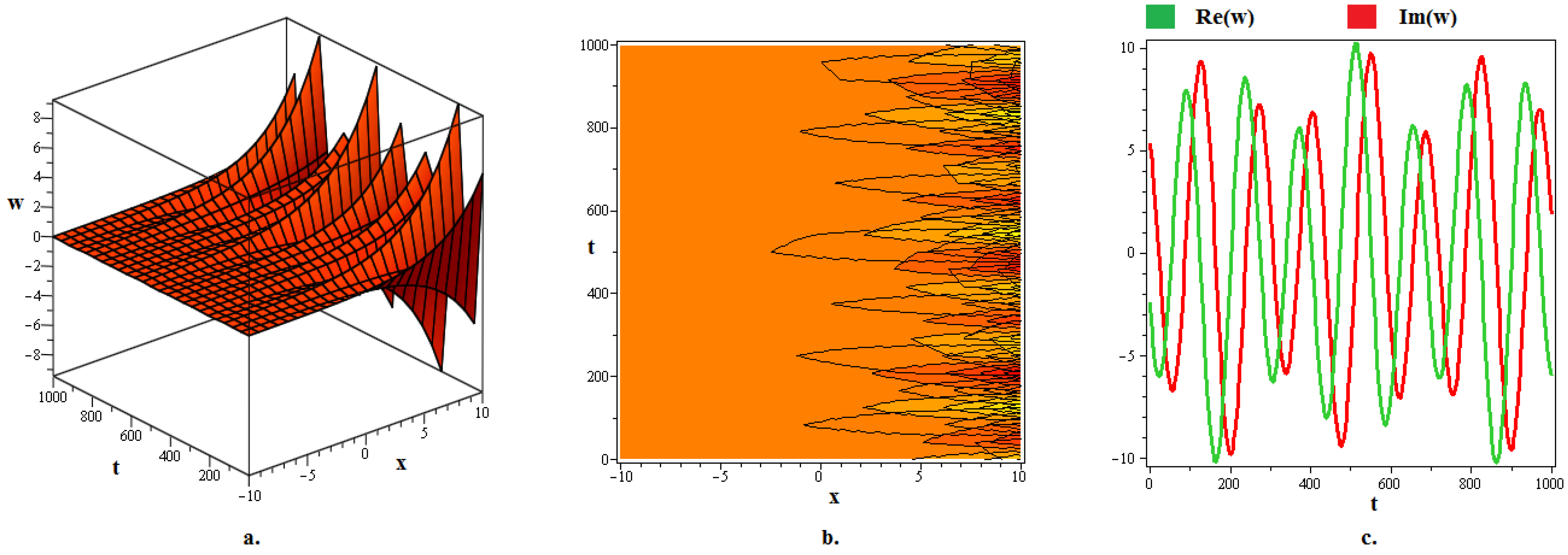
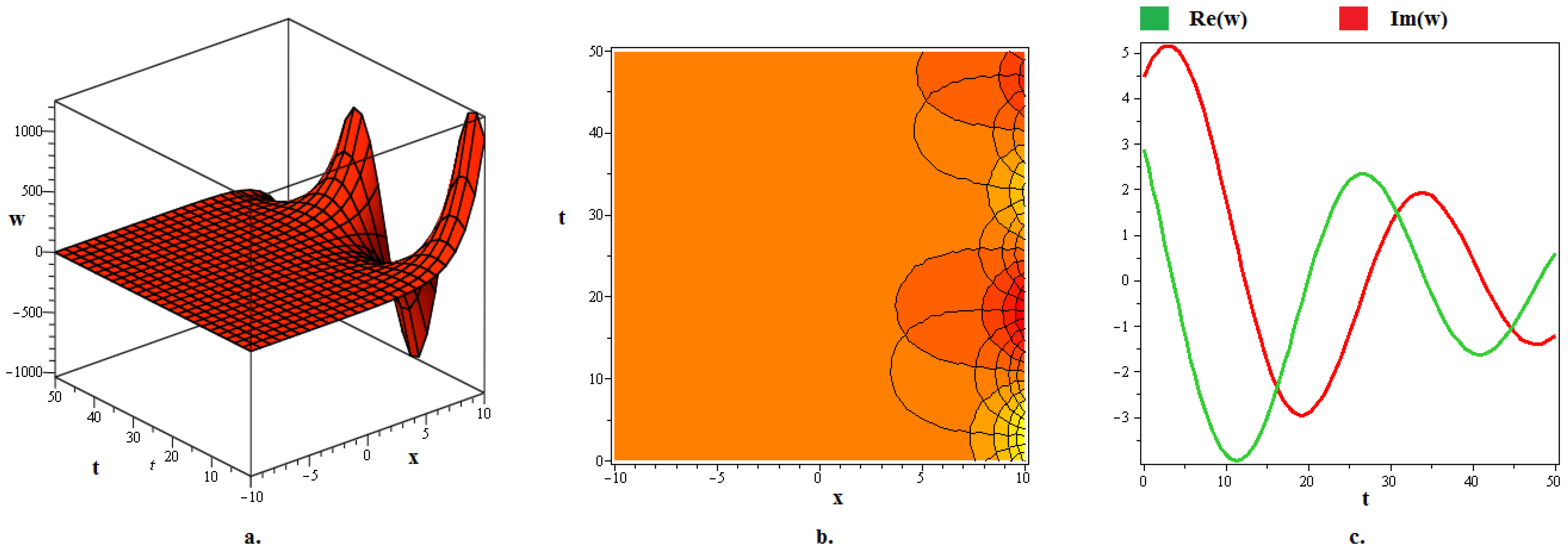
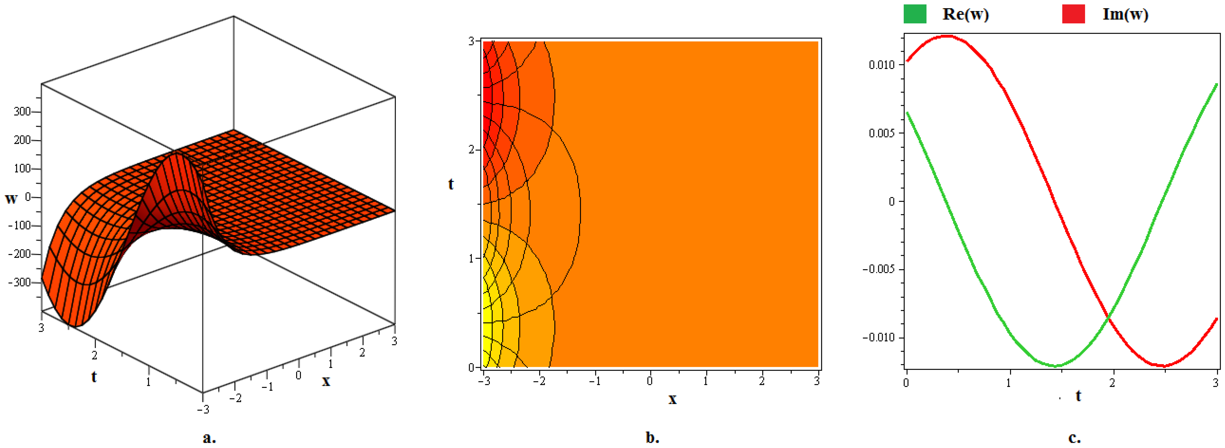
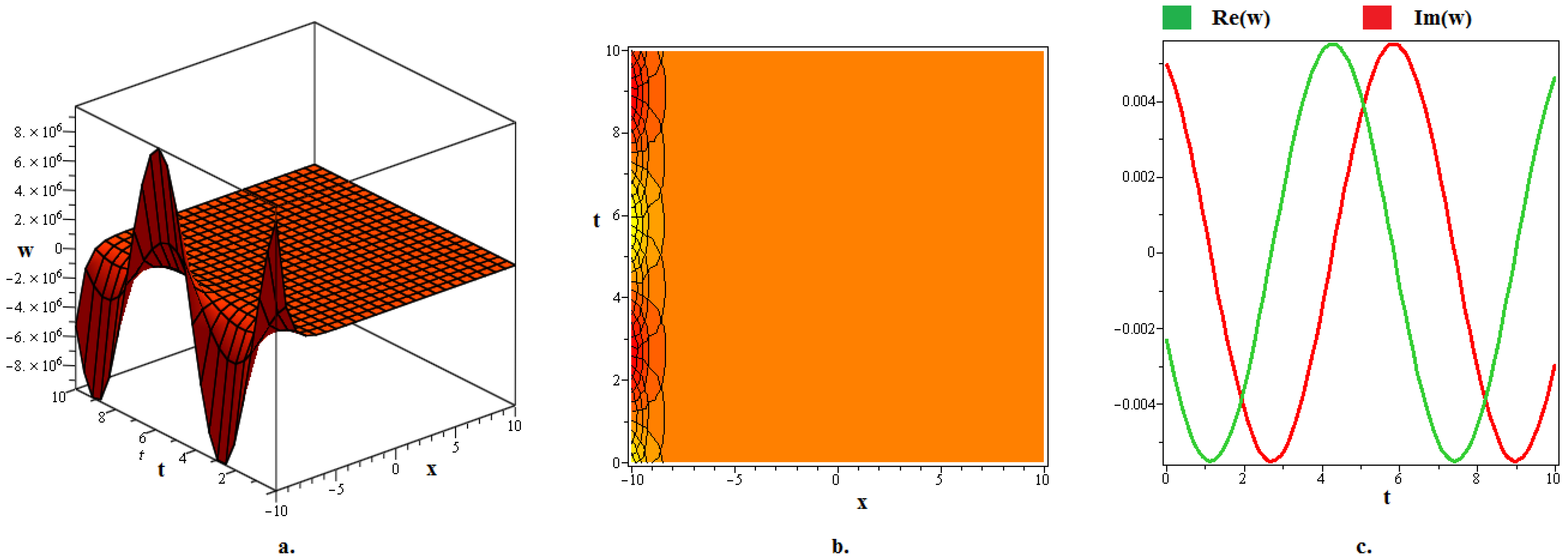
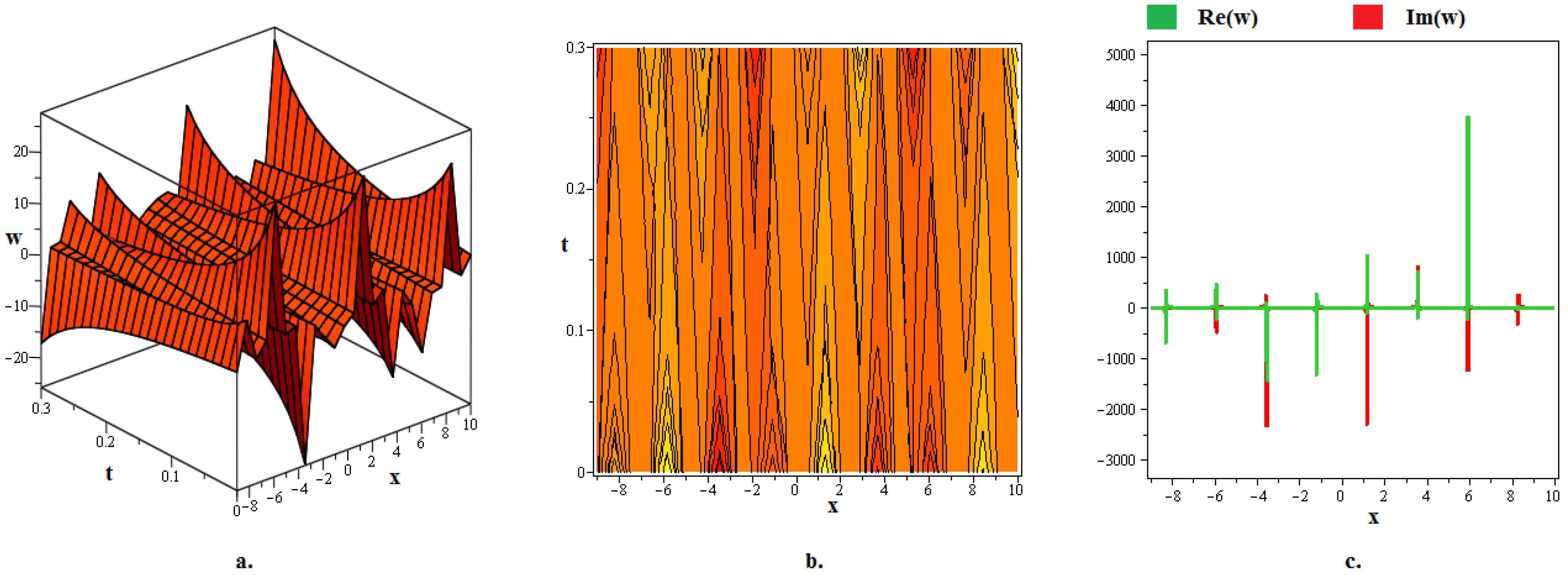
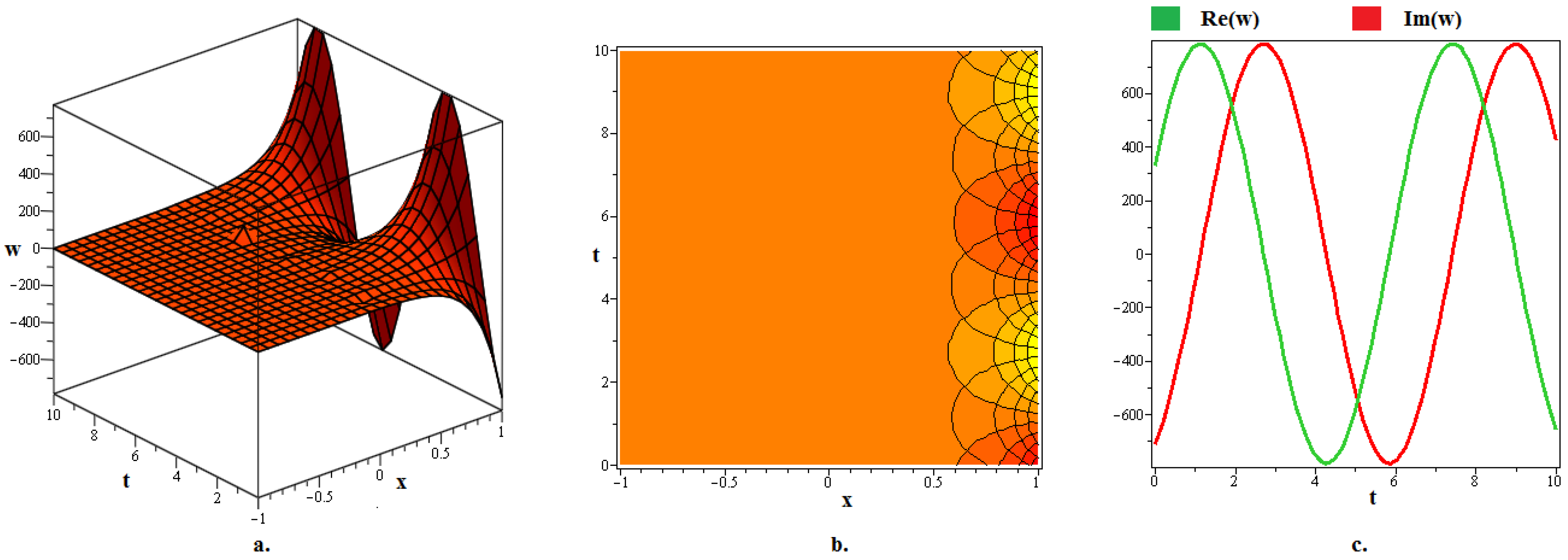
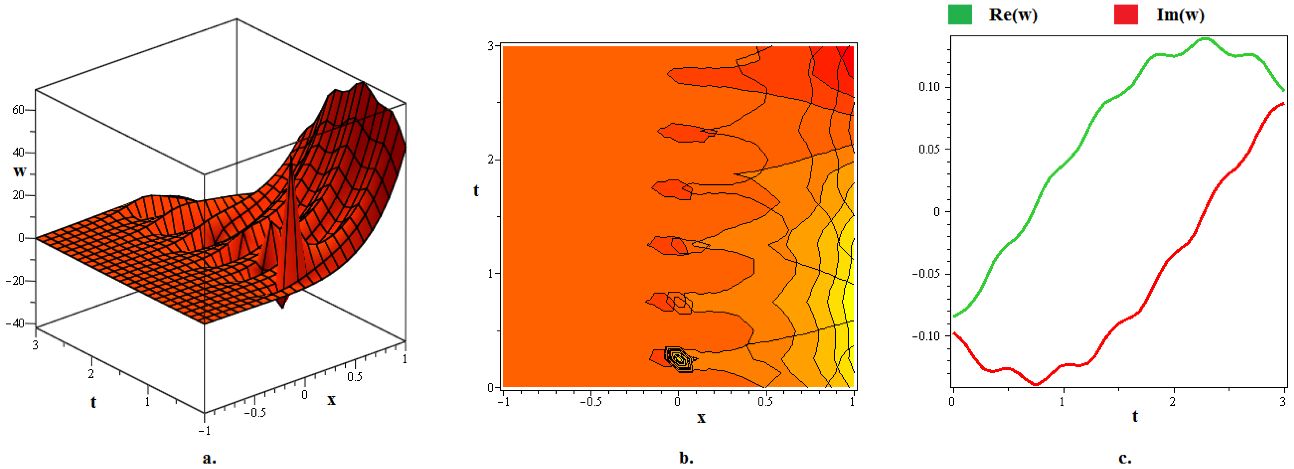
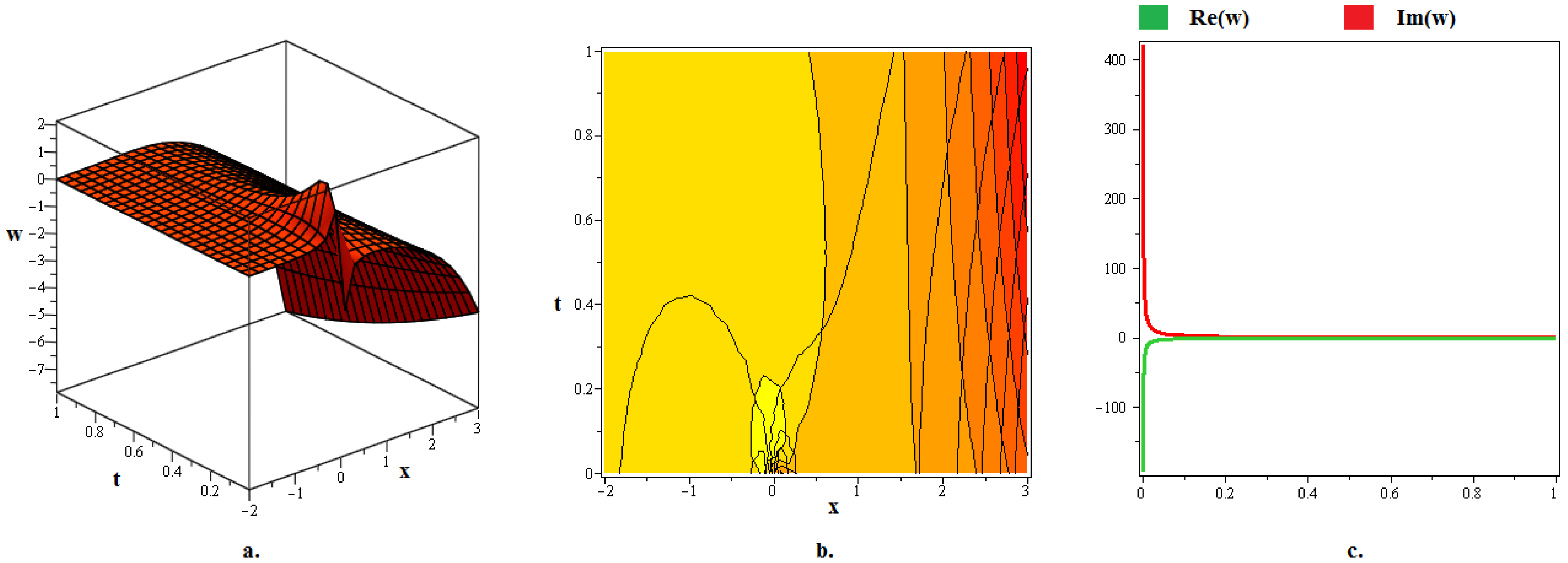
4. Discussion and Graphs

In this section of the study, we discuss various optical wave forms that were found in the model. We were able to extract and vividly exhibit optical solitons’ wave patterns in 3D, contour, and 2D formats using RMESEMs. Our comprehension of the dynamics of optical pulse theory in optical fibers may be greatly advanced by the developed optical soliton solutions. Additionally, the optical solitons in the context of CNHEs were shown to visually illustrate how certain limitation conditions cause them to lose stability as they approach an axis, exhibiting periodic axial disturbances and ultimately forming optical fractals. This periodic behaviour of the soliton may also be attributed to the formation of a Duffing equation as stated in (9) from the CNHEs, after the implementation of a complex transformation since a Duffing equation possesses periodic solutions [38]. An optical soliton, as found in the context of CNHEs, is a self-sustaining waveform that travels through fiber optic media without changing its speed and shape. These waves are renowned for their capacity to rebuild and stabilize themselves following a collision with other waves of a similar nature. Nevertheless, our analysis showed that the presence of external forces and the dispersion of nonlinearity cause axial and periodic disturbances in the generated solitons which results in the formation of optical fractals because this chaotic perturbation induces instabilities in the soliton. However, in some of our solitons, the fractal shape has also formed due to the soliton interaction (particularly with singular lumps) and self similarities. Singularities can arise in the setting of CNHEs because of the nonlinear interplay and complex parameter dependencies inside the non-integrable system, especially when periodic and axial perturbations affect the optical solitons. Singular points or localized spikes in the solution may result from these perturbations, which have the potential to destabilize the optical soliton. Furthermore, our proposed RMESEM demonstrates its usefulness by broadening the spectrum of optical soliton solutions, offering important insights into the dynamics of the CNHEs, and suggesting possible applications in the management of nonlinear models. Figure 1, the (a) 3D graph, (b) contour graph, and (c) 2D graph (when $x=10$) represent the optical soliton solution $u_{1,5}(t,x)$ articulated in (20) for $\rho :=4,\varrho :=5,\sigma :=1,\phi :=0.25\times {10}^{-2},k_2:=0.45\times {10}^{-1},k_3:=0.2\times {10}^{-1},\nu :=2,d_0:=1$. In this depiction, the optical fractal is formed due to the chaotic axial perturbation. Figure 2, the (a) 3D graph, (b) contour graph, and (c) 2D graph (when $x=1$) represent the optical soliton solution $u_{1,9}(t,x)$ articulated in (24) for $\rho :=1,\varrho :=2,\sigma :=1,\phi :=0.15\times {10}^{-2},k_2:=0.235,k_3:=0.124,\nu :=1,d_0:=3$. In this depiction, the optical fractal is formed due to the periodic axial perturbation. Figure 3, the (a) 3D graph, (b) contour graph, and (c) 2D graph (when $x=1.5$) represent the optical soliton solution $u_{1,11}(t,x)$ articulated in (26) for $\rho :=6,\varrho :=3,\sigma :=0,\phi :=0.95\times {10}^{-3},k_2:=0.445,k_3:=0.66,\nu :=4,d_0:=1,b:=2,\mu :=3$. In this depiction, the optical fractal is formed due to the chaotic periodic axial perturbation. Figure 4, the (a) 3D graph, (b) contour graph, and (c) 2D graph (when $x=3$) represent the optical soliton solution $u_{2,4}(t,x)$ articulated in (30) for $\rho :=2,\varrho :=10,\sigma :=8,\phi :=0.15\times {10}^{-2},k_3:=0,k_2:=1.5,\nu :=1,c_2:=1,c_0:=2,d_0:=1$. In this depiction, the optical fractal is formed due to the periodic axial perturbation. Figure 5, the (a) 3D graph, (b) contour graph, and (c) 2D graph (when $x=5$) represent the optical soliton solution $u_{2,8}(t,x)$ articulated in (34) for $\rho :=0,\varrho :=1,\sigma :=-2,\phi :=0.75\times {10}^{-2},k_3:=0,k_2:=1,\nu :=2,c_2:=2,c_0:=3,d_0:=1,\mu :=1,b:=-2$. In this depiction, the optical fractal is formed due to the periodic axial perturbation. Figure 6, the (a) 3D graph, (b) contour graph, and (c) 2D graph (when $t=0$) represent the optical soliton solution $u_{3,1}(t,x)$ articulated in (37) for $\rho :=1,\varrho :=1,\sigma :=4,\phi :=0.1\times {10}^{-3},k_3:=0.685,k_2:=0.115,\nu :=1,c_2:=2$. In this depiction, the optical fractal is formed due to the chaotic bi-axial perturbation. Figure 7, the (a) 3D graph, (b) contour graph, and (c) 2D graph (when $x=1$) represent the optical soliton solution $u_{3,5}(t,x)$ articulated in (41) for $\rho :=1,\varrho :=10,\sigma :=9,\phi :=0.35\times {10}^{-2},k_3:=1,k_2:=1,\nu :=2,c_2:=1$. In this depiction, the optical fractal is formed due to the periodic axial perturbation. Figure 8, the (a) 3D graph, (b) contour graph, and (c) 2D graph (when $x=-1$) represent the optical soliton solution $u_{3,13}(t,x)$ articulated in (49) for $\rho :=0,\varrho :=2,\sigma :=5,\phi :=0.22\times {10}^{-2},k_3:=2,k_2:=1,\nu :=4,c_2:=3,z_2:=1$. In this depiction, the optical fractal is formed due to the chaotic axial perturbation.

Figure 9, the (a) 3D graph, (b) contour graph, and (c) 2D graph (when $x=0$) represent the optical soliton solution $u_{4,9}(t,x)$ articulated in (59) for $\rho :=4,\varrho :=4,\sigma :=1,\phi :=0.15\times {10}^{-2},k_3:=2,k_2:=1,\nu :=2,c_2:=3,z_2:=5,{\kappa }_2:=1,{\kappa }_2:=4$. In this depiction, the optical fractal is formed due to the chaotic axial perturbation of the optical lump. Figure 10, the (a) 3D graph, (b) contour graph, and (c) 2D graph (when $x=0$) represent the optical soliton solution $u_{4,14}(t,x)$ articulated in (64) for $\rho :=0,\varrho :=1,\sigma :=3,\phi :=0.45\times {10}^{-2},k_3:=3,k_2:=2,\nu :=5,c_2:=1,z_2:=4,{\kappa }_2:=2,{\kappa }_2:=1$. In this depiction, the optical fractal is formed due to the chaotic axial perturbation of the singular lump.

5. Conclusions

In this work, we used the effective RMESEM to create and analyze novel optical soliton solutions for CNHEs in the form of exponential, rational, trigonometric, hyperbolic, and rational hyperbolic functions. We also offered some 3D, contour, and 2D plots for the free selections of the physical parameters to more clearly show the propagating behaviours of the produced optical solitons. These visuals reveal that, when acquired optical solitons approach an axis, they lose stability under specific constraint conditions and exhibit periodic axial perturbations, resulting in the formation of optical fractals. There are several practical uses for the produced optical solitons in the fields of optics. Moreover, our hired RMESEM also proves its efficacy by expanding the range of optical soliton solutions, providing valuable insights into the CNHE dynamics, and indicating potential uses in addressing nonlinear models. While the RMESEM has significantly improved our understanding of soliton dynamics and their relationship to the models under investigation, it is important to acknowledge the limitations of this method; particularly, this method fails when the greatest derivative and nonlinear term are not balanced homogeneously. Notwithstanding this limitation, the present investigation demonstrates that the methodology employed in this work is extremely dependable, transferable, and productive for nonlinear problems in a variety of natural science domains. Moreover, the future goal of this investigation is to delve into the sensitiveness of fractal solitons, the incorporation and impact of the fractional derivatives on fractal solitons, and the calculation of scaling factors of fractal theory.

References

1. Abdelrahman, M.A.; Mohammed, W.W.; Alesemi, M.; Albosaily, S. The effect of multiplicative noise on the exact solutions of nonlinear Schrödinger equation. AIMS Math. 2021, 6, 2970–2980. [Google Scholar] [CrossRef]
2. Alomair, R.A.; Hassan, S.Z.; Abdelrahman, M.A. A new structure of solutions to the coupled nonlinear Maccari’s systems in plasma physics. AIMS Math. 2020, 7, 8588–8606. [Google Scholar] [CrossRef]
3. Navier, C.L. Navier Stokes Equation; Chez Carilian-Goeury: Paris, France, 1838. [Google Scholar]
4. Hafez, M.G.; Alam, M.N.; Akbar, M.A. Traveling wave solutions for some important coupled nonlinear physical models via the coupled Higgs equation and the Maccari system. J. King Saud-Univ.-Sci. 2015, 27, 105–112. [Google Scholar] [CrossRef]
5. El-Naggar, A.M.; Ismail, G.M. Analytical solution of strongly nonlinear Duffing oscillators. Alex. Eng. J. 2016, 55, 1581–1585. [Google Scholar] [CrossRef]
6. Xiao, Y.; Barak, S.; Hleili, M.; Shah, K. Exploring the dynamical behaviour of optical solitons in integrable kairat-II and kairat-X equations. Phys. Scr. 2024, 99, 095261. [Google Scholar] [CrossRef]
7. Ali, R.; Barak, S.; Altalbe, A. Analytical study of soliton dynamics in the realm of fractional extended shallow water wave equations. Phys. Scr. 2024, 99, 065235. [Google Scholar] [CrossRef]
8. Akbar, M.A.; Akinyemi, L.; Yao, S.W.; Jhangeer, A.; Rezazadeh, H.; Khater, M.M.; Ahmad, H.; Mustafa Inc. Soliton solutions to the Boussinesq equation through sine-Gordon method and Kudryashov method. Results Phys. 2021, 25, 104228. [Google Scholar] [CrossRef]
9. Yang, X.F.; Deng, Z.C.; Wei, Y. A Riccati-Bernoulli sub-ODE method for nonlinear partial differential equations and its application. Adv. Differ. Equ. 2015, 2015, 117. [Google Scholar] [CrossRef]
10. Khan, H.; Barak, S.; Kumam, P.; Arif, M. Analytical solutions of fractional Klein-Gordon and gas dynamics equations, via the (G′/G)-expansion method. Symmetry 2019, 11, 566. [Google Scholar] [CrossRef]
11. Khan, H.; Baleanu, D.; Kumam, P.; Al-Zaidy, J.F. Families of travelling waves solutions for fractional-order extended shallow water wave equations, using an innovative analytical method. IEEE Access 2019, 7, 107523–107532. [Google Scholar] [CrossRef]
12. Hammad, M.M.A.; Shah, R.; Alotaibi, B.M.; Alotiby, M.; Tiofack, C.G.L.; Alrowaily, A.W.; El-Tantawy, S.A. On the modified versions of ( G G ) -expansion technique for analyzing the fractional coupled Higgs system. AIP Adv. 2013, 13, 105131. [Google Scholar] [CrossRef]
13. Ali, R.; Tag-eldin, E. A comparative analysis of generalized and extended ( G G ) -Expansion methods for travelling wave solutions of fractional Maccari’s system with complex structure. Alex. Eng. J. 2023, 79, 508–530. [Google Scholar] [CrossRef]
14. He, J.H.; Wu, X.H. Exp-function method for nonlinear wave equations. Chaos Solitons Fractals 2006, 30, 700–708. [Google Scholar] [CrossRef]
15. Cinar, M.; Secer, A.; Ozisik, M.; Bayram, M. Derivation of optical solitons of dimensionless Fokas-Lenells equation with perturbation term using Sardar sub-equation method. Opt. Quantum Electron. 2022, 54, 402. [Google Scholar] [CrossRef]
16. Barman, H.K.; Islam, M.E.; Akbar, M.A. A study on the compatibility of the generalized Kudryashov method to determine wave solutions. Propuls. Power Res. 2021, 10, 95–105. [Google Scholar] [CrossRef]
17. Shi-qiang, D. Poincare-Lighthill-Kuo method and symbolic computation. Appl. Math. Mech. 2001, 22, 261–269. [Google Scholar] [CrossRef]
18. Hietarinta, J. Introduction to the Hirota bilinear method. In Integrability of Nonlinear Systems, Proceedings of the CIMPA School Pondicherry University, India, 8–26 January 1996; Springer: Berlin/Heidelberg, Germany, 2007; pp. 95–103. [Google Scholar]
19. Bilal, M.; Iqbal, J.; Ali, R.; Awwad, F.A.; AIsmail, E.A. Exploring Families of Solitary Wave Solutions for the Fractional Coupled Higgs System Using Modified Extended Direct Algebraic Method. Fractal Fract. 2023, 7, 653. [Google Scholar] [CrossRef]
20. Aldandani, M.; Altherwi, A.A.; Abushaega, M.M. Propagation patterns of dromion and other solitons in nonlinear Phi-Four (ϕ4) equation. AIMS Math. 2024, 9, 19786–19811. [Google Scholar] [CrossRef]
21. Mirzazadeh, M. Modified simple equation method and its applications to nonlinear partial differential equations. Inf. Sci. Lett. 2014, 3, 1. [Google Scholar] [CrossRef]
22. Zayed, E.M.E.; Al-Nowehy, A.G. The Modified Simple Equation Method, the Exp-Function Method, and the Method of Soliton Ansatz for Solving the Long-Short Wave Resonance Equations. Z. Naturforschung A 2016, 71, 103–112. [Google Scholar] [CrossRef]
23. Kudryashov, N.A. Seven common errors in finding exact solutions of nonlinear differential equations. Commun. Nonlinear Sci. Numer. Simul. 2009, 14, 3507–3529. [Google Scholar] [CrossRef]
24. Navickas, Z.; Ragulskis, M. Comments on “A new algorithm for automatic computation of solitary wave solutions to nonlinear partial differential equations based on the Exp-function method”. Appl. Math. Comput. 2014, 243, 419–425. [Google Scholar] [CrossRef]
25. Antonova, A.O.; Kudryashov, N.A. Generalization of the simplest equation method for nonlinear non-autonomous differential equations. Commun. Nonlinear Sci. Numer. Simul. 2014, 19, 4037–4041. [Google Scholar] [CrossRef]
26. Navickas, Z.; Marcinkevicius, R.; Telksniene, I.; Telksnys, T.; Ragulskis, M. Structural stability of the hepatitis C model with the proliferation of infected and uninfected hepatocytes. Math. Comput. Model. Dyn. Syst. 2024, 30, 51–72. [Google Scholar] [CrossRef]
27. Martin-Vergara, F.; Rus, F.; Villatoro, F.R. Fractal structure of the soliton scattering for the graphene superlattice equation. Chaos Solitons Fractals 2021, 151, 111281. [Google Scholar] [CrossRef]
28. Wang, K. A new fractal model for the soliton motion in a microgravity space. Int. J. Numer. Methods Heat Fluid Flow 2021, 31, 442–451. [Google Scholar] [CrossRef]
29. Zheng, C.L. Coherent soliton structures with chaotic and fractal behaviors in a generalized (2+ 1)-dimensional Korteweg de-Vries system. Chin. J. Phys. 2003, 41, 442–455. [Google Scholar]
30. Bunde, A.; Havlin, S. (Eds.) Fractals in Science; Springer: Berlin/Heidelberg, Germany, 2013. [Google Scholar]
31. Stanley, H.E. Fractal landscapes in physics and biology. Phys. Stat. Mech. Its Appl. 1992, 186, 1–32. [Google Scholar] [CrossRef]
32. Bizzarri, M.; Giuliani, A.; Cucina, A.; D’Anselmi, F.; Soto, A.M.; Sonnenschein, C. Fractal analysis in a systems biology approach to cancer. In Seminars in Cancer Biology; Academic Press: Cambridge, MA, USA, 2011; Volume 21, pp. 175–182. [Google Scholar]
33. Abraham, N.B.; Firth, W.J. Overview of transverse effects in nonlinear-optical systems. JOSA B 1990, 7, 951–962. [Google Scholar] [CrossRef]
34. Alsaud, H.; Youssoufa, M.; Inc, M.; Inan, I.E.; Bicer, H. Some optical solitons and modulation instability analysis of (3+ 1)-dimensional nonlinear Schrödinger and coupled nonlinear Helmholtz equations. Opt. Quantum Electron. 2024, 56, 1138. [Google Scholar] [CrossRef]
35. Tamilselvan, K.; Kanna, T.; Khare, A. Nonparaxial elliptic waves and solitary waves in coupled nonlinear Helmholtz equations. Commun. Nonlinear Sci. Numer. Simul. 2016, 39, 134–148. [Google Scholar] [CrossRef]
36. Singh, S.; Kaur, L.; Sakthivel, R.; Murugesan, K. Computing solitary wave solutions of coupled nonlinear Hirota and Helmholtz equations. Phys. Stat. Mech. Its Appl. 2020, 560, 125114. [Google Scholar] [CrossRef]
37. Saha, N.; Roy, B.; Khare, A. Coupled Helmholtz equations: Chirped solitary waves. Chaos Interdiscip. J. Nonlinear Sci. 2021, 31, 113104. [Google Scholar] [CrossRef] [PubMed]
38. Yamaguti, M.; Yoshihara, H.; Niahida, T. Periodic solutions of Duffing equation. CiNii J. 1988, 673, 80–95. [Google Scholar]
Figure 1. The (a) 3D graph, (b) contour graph, and (c) 2D graph (when x = 10 ) represent the optical soliton solution u 1 , 5 ( t , x ) articulated in (20) for ρ : = 4 , ϱ : = 5 , σ : = 1 , φ : = 0.25 × 10 2 , k 2 : = 0.45 × 10 1 , k 3 : = 0.2 × 10 1 , ν : = 2 , d 0 : = 1 . In this depiction, the optical fractal is formed due to the chaotic axial perturbation.
Fractalfract 08 00594 g001
Figure 2. The (a) 3D graph, (b) contour graph, and (c) 2D graph (when x = 1 ) represent the optical soliton solution u 1 , 9 ( t , x ) articulated in (24) for ρ : = 1 , ϱ : = 2 , σ : = 1 , φ : = 0.15 × 10 2 , k 2 : = 0.235 , k 3 : = 0.124 , ν : = 1 , d 0 : = 3 . In this depiction, the optical fractal is formed due to the periodic axial perturbation.
Fractalfract 08 00594 g002
Figure 3. The (a) 3D graph, (b) contour graph, and (c) 2D graph (when x = 1.5 ) represent the optical soliton solution u 1 , 11 ( t , x ) articulated in (26) for ρ : = 6 , ϱ : = 3 , σ : = 0 , φ : = 0.95 × 10 3 , k 2 : = 0.445 , k 3 : = 0.66 , ν : = 4 , d 0 : = 1 , b : = 2 , μ : = 3 . In this depiction, the optical fractal is formed due to the chaotic periodic axial perturbation.
Fractalfract 08 00594 g003
Figure 4. The (a) 3D graph, (b) contour graph, and (c) 2D graph (when x = 3 ) represent the optical soliton solution u 2 , 4 ( t , x ) articulated in (30) for ρ : = 2 , ϱ : = 10 , σ : = 8 , φ : = 0.15 × 10 2 , k 3 : = 0 , k 2 : = 1.5 , ν : = 1 , c 2 : = 1 , c 0 : = 2 , d 0 : = 1 . In this depiction, the optical fractal is formed due to the periodic axial perturbation.
Fractalfract 08 00594 g004
Figure 5. The (a) 3D graph, (b) contour graph, and (c) 2D graph (when x = 5 ) represent the optical soliton solution u 2 , 8 ( t , x ) articulated in (34) for ρ : = 0 , ϱ : = 1 , σ : = 2 , φ : = 0.75 × 10 2 , k 3 : = 0 , k 2 : = 1 , ν : = 2 , c 2 : = 2 , c 0 : = 3 , d 0 : = 1 , μ : = 1 , b : = 2 . In this depiction, the optical fractal is formed due to the periodic axial perturbation.
Fractalfract 08 00594 g005
Figure 6. The (a) 3D graph, (b) contour graph, and (c) 2D graph (when t = 0 ) represent the optical soliton solution u 3 , 1 ( t , x ) articulated in (37) for ρ : = 1 , ϱ : = 1 , σ : = 4 , φ : = 0.1 × 10 3 , k 3 : = 0.685 , k 2 : = 0.115 , ν : = 1 , c 2 : = 2 . In this depiction, the optical fractal is formed due to the chaotic bi-axial perturbation.
Fractalfract 08 00594 g006
Figure 7. The (a) 3D graph, (b) contour graph, and (c) 2D graph (when x = 1 ) represent the optical soliton solution u 3 , 5 ( t , x ) articulated in (41) for ρ : = 1 , ϱ : = 10 , σ : = 9 , φ : = 0.35 × 10 2 , k 3 : = 1 , k 2 : = 1 , ν : = 2 , c 2 : = 1 . In this depiction, the optical fractal is formed due to the periodic axial perturbation.
Fractalfract 08 00594 g007
Figure 8. The (a) 3D graph, (b) contour graph, and (c) 2D graph (when x = 1 ) represent the optical soliton solution u 3 , 13 ( t , x ) articulated in (49) for ρ : = 0 , ϱ : = 2 , σ : = 5 , φ : = 0.22 × 10 2 , k 3 : = 2 , k 2 : = 1 , ν : = 4 , c 2 : = 3 , z 2 : = 1 . In this depiction, the optical fractal is formed due to the chaotic axial perturbation.
Fractalfract 08 00594 g008