Compact ADI Difference Scheme for the 2D Time Fractional Nonlinear Schrödinger Equation

Abstract

In this paper, we will introduce a compact alternating direction implicit (ADI) difference scheme for solving the two-dimensional (2D) time fractional nonlinear Schrödinger equation. The difference scheme is constructed by using the $L1-2-3$ formula to approximate the Caputo fractional derivative in time and the fourth-order compact difference scheme is adopted in the space direction. The proposed difference scheme with a convergence accuracy of $O({\tau }^{1+\alpha }+h_x^4+h_y^4)(\alpha \in (0,1))$ is obtained by adding a small term, where $\tau$, $h_x$, $h_y$ are the temporal and spatial step sizes, respectively. The convergence and unconditional stability of the difference scheme are obtained. Moreover, numerical experiments are given to verify the accuracy and efficiency of the difference scheme.

1. Introduction

The Schrödinger equation, as a basic equation in quantum mechanics, is widely used in plasma physics, nonlinear photonics, water waves, bimolecular dynamics, and other fields. Models with fractional derivatives are better at describing the motion of things in real situations. In 2004, the time fractional Schrödinger equation is proposed in [1], which is considered by changing the first-order derivative to a Caputo fractional derivative. Various nonlinear development equations are discussed in [2], and finite difference schemes are used to solve these equations. This approach is also applied to the nonlinear Schrödinger equation.

In this paper, we will discuss the following 2D time fractional nonlinear Shrödinger equation (TFNSE) [3] with the Caputo fractional derivative:

$$\left\{\begin{array}{c}i{\displaystyle \frac{{\partial }^{\alpha }u(x,y,t)}{\partial t^{\alpha }}}=\left({\displaystyle \frac{{\partial }^2}{\partial x^2}}+{\displaystyle \frac{{\partial }^2}{\partial y^2}}\right)u\left(x,y,t\right)+f\left({\left|u\left(x,y,t\right)\right|}^2\right)u\left(x,y,t\right),(x,y)\in \Omega ,t\in (0,T],\hfill \\ u\left(x,y,0\right)=u_0\left(x,y\right),(x,y)\in \Omega ,\hfill \\ u\left(x,y,t\right)=0,(x,y,t)\in \partial \Omega \times (0,T],\hfill \end{array}\right.$$

(1)

here, $u_0(x,y),f$ are the given smooth functions, $i=\sqrt{-1}$, $\Omega =[0,L_x]\times [0,L_y]$ represents the domin and $\partial \Omega$ is the boundary. The $\alpha$-order Caputo fractional derivative [4] is defined by

$${\mathcal{D}}_t^{\alpha }u\left(t\right)={\displaystyle \frac{1}{\Gamma (1-\alpha )}}{\int }_0^t{\displaystyle \frac{u^{\prime }\left(s\right)}{{(t-s)}^{\alpha }}}ds,$$

(2)

with $\alpha \in (0,1)$.

For Equation (2), this paper will apply the time-fractional Schrödinger equation, which is classified as an integral-differential equation. Due to the challenges in obtaining an analytical solution, the use of numerical methods to address the time-fractional Schrödinger equation has emerged as a widely debated and significant topic. The $L2-1$ formula is proposed in [5] for approximating the $\alpha$-order Caputo fractional derivative for solving time-fractional sub-diffusion equation. The $L2-1\sigma$ formula is proposed in [6,7] for the time-fractional reaction sub-diffusion equation. Further, the $L2$ formula is proposed for Caputo-type time-fractional sub-diffusion equations in [8]. The paper [9] focused on a conservative implicit difference scheme for one dimensional nonlinear Schrödinger equation by presupposing a higher-order difference scheme, and proving its stability and convergence with second-order accuracy in time and fourth-order accuracy in space.

In order to obtain high-order accuracy and reduce the cost of computation, this article will discuss a compact ADI scheme in the space direction for Equation (1). A compact ADI scheme is proposed in [10] for the 2D fractional sub-diffusion equation, and the error of the compact scheme is discussed. Based on previous papers, a new ADI scheme is introduced in [11] for solving three-dimensional parabolic equations. And a compact difference scheme for solving the nonlinear time-space fractional Schrödinger equation is discussed in [12], it is also proved that the scheme has second-order accuracy in time and space directions. And a new high order ADI numerical difference formula is discussed in [13] for a time-fractional convection–diffusion equation. In [14], several high-order compact finite difference schemes are presented and analyzed for the numerical solution of one and two-dimensional linear time fractional Schrödinger equations. The time Caputo fractional derivative is approximated using the $L1$ and $L1-2$ formula. Spatial discretization employs a fourth-order compact finite difference method. Furthermore, the unconditional stability of the proposed scheme is examined using Fourier analysis.

The following sections of this paper are organized as follows. Section 2 is devoted to some notations and useful lemmas. In Section 3, the derivation of the compact ADI difference scheme is discussed for Equation (1). The convergence and stability are analyzed seriously in Section 4. In Section 5, some numerical experiments are given to illustrate the efficiency of the scheme which introduced in this work. Finally, the paper ends with a conclusion section.

2. Preliminaries

We first introduce some notations used in this paper. $M_x$, $M_y$, and N are the spatial and temporal partition parameters, respectively, and are the positive integers. We set the spatial step size as $h_x=L_x/M_x$, $h_y=L_y/M_y$ and the time step size as $\tau =T/N$. Denote $x_j=j{h}_x(j=0,1,2,\cdots ,M_x)$, $y_k=k{h}_y(k=0,1,2,\cdots ,M_y)$, $t_n=n\tau (n=0,1,2,\cdots ,N)$, $h_x=h_y=h$. Suppose $\tilde{U}=u_{jk}^n$ is a grid function on $\overline{\Omega }(\overline{\Omega }=\Omega \times [0,T])$, and ${\overline{u}}_{jk}^n$ is a conjugate function of $u_{jk}^n$, for any $u,v\in \tilde{U}$, given the discrete notation as follows:

$$\begin{array}{c}{\delta }_x{u}_{j+{\displaystyle \frac{1}{2}},k}={\displaystyle \frac{u_{j+1,k}-u_{j,k}}{h_x}},{\delta }_x^2{u}_{jk}={\displaystyle \frac{u_{j-1,k}-2u_{jk}+u_{j+1,k}}{h_x^2}},H_x{u}_{jk}=\left(1+{\displaystyle \frac{h_x^2}{12}}{\delta }_x^2\right)u_{jk},\\ {\delta }_y{u}_{j,k+{\displaystyle \frac{1}{2}}}={\displaystyle \frac{u_{j,k+1}-u_{j,k}}{h_y}},{\delta }_y^2{u}_{jk}={\displaystyle \frac{u_{j,k-1}-2u_{jk}+u_{j,k+1}}{h_y^2}},H_y{u}_{jk}=\left(1+{\displaystyle \frac{h_y^2}{12}}{\delta }_y^2\right)u_{jk},\\ (u,v)=h_x{h}_y\sum _{j=1}^{M_x-1}\sum _{k=1}^{M_y-1}{u}_{jk}{\overline{v}}_{jk},\left|\right|u\left|\right|=\sqrt{(u,u)}{,\left|\right|u\left|\right|}_{\infty }=\underset{1\le j\le M_x-1,1\le k\le M_y-1}{max}\left|u_{jk}\right|,\\ ({\delta }_{x}u,{\delta }_{x}v)=h_x{h}_y\sum _{j=0}^{M_x-1}\sum _{k=0}^{M_y-1}({\delta }_x{u}_{j+{\displaystyle \frac{1}{2}},k})({\delta }_x{\overline{v}}_{j+{\displaystyle \frac{1}{2}},k}),\left|\right|{\delta }_{x}u{\left|\right|}^2=({\delta }_{x}u,{\delta }_{x}u),\\ ({\delta }_{y}u,{\delta }_{y}v)=h_x{h}_y\sum _{j=0}^{M_x-1}\sum _{k=0}^{M_y-1}({\delta }_y{u}_{j,k+{\displaystyle \frac{1}{2}}})({\delta }_y{\overline{v}}_{j,k+{\displaystyle \frac{1}{2}}}),\left|\right|{\delta }_{y}u{\left|\right|}^2=({\delta }_{y}u,{\delta }_{y}u),\\ {\Delta }_h{u}_{jk}={\delta }_x^2{u}_{jk}+{\delta }_y^2{u}_{jk},\left|\right|{\nabla }_{h}u{\left|\right|}^2=({\delta }_{x}u,{\delta }_{x}u)+({\delta }_{y}u,{\delta }_{y}u).\end{array}$$

Definition 1 

(Formula $L1-2-3$ [15]). Assume that $0<\alpha <1$, $u\left(t\right)\in C^4[0,T]$, then

$$\begin{array}{cc}\hfill {}_0{}^C\mathcal{D}_t^{\alpha }u\left(t^n\right)=& {\displaystyle \frac{1}{{\tau }^{\alpha }\Gamma (2-\alpha )}}\left[{\varpi }_0{u}^n-\sum _{\gamma =1}^{n-1}({\varpi }_{n-\gamma -1}-{\varpi }_{n-\gamma })u^{\gamma }-{\varpi }_{n-1}{u}^0\right],\hfill \end{array}$$

when $n=1$, ${\varpi }_0=1$. When $n=2$,

$${\varpi }_{\gamma }=\left\{\begin{array}{cc}{p}_{\gamma }+q_{\gamma },\hfill & \gamma =0,\hfill \\ p_{\gamma }-q_{\gamma -1},\hfill & \gamma =1.\hfill \end{array}\right.$$

When $n=3$,

$${\varpi }_{\gamma }=\left\{\begin{array}{cc}{p}_{\gamma }+q_{\gamma }+r_{\gamma },\hfill & \gamma =0,\hfill \\ p_{\gamma }+q_{\gamma }-q_{\gamma -1}-2r_{\gamma -1},\hfill & \gamma =1,\hfill \\ p_{\gamma }-q_{\gamma -1}+r_{\gamma -2},\hfill & \gamma =2,\hfill \end{array}\right.$$

and when $n⩾4$,

$${\varpi }_{\gamma }=\left\{\begin{array}{cc}{p}_{\gamma }+q_{\gamma }+r_{\gamma },\hfill & \gamma =0,\hfill \\ p_{\gamma }+q_{\gamma }-q_{\gamma -1}+r_{\gamma }-2r_{\gamma -1},\hfill & \gamma =1,\hfill \\ p_{\gamma }+q_{\gamma }-q_{\gamma -1}+r_{\gamma }-2r_{\gamma -1}+r_{\gamma -2},\hfill & 2⩽\gamma ⩽n-3,\hfill \\ p_{\gamma }+q_{\gamma }-q_{\gamma -1}-2r_{\gamma -1}+r_{\gamma -2},\hfill & \gamma =n-2,\hfill \\ p_{\gamma }-q_{\gamma -1}+r_{\gamma -2},\hfill & \gamma =n-1,\hfill \end{array}\right.$$

where

$$\begin{array}{c}{p}_{\gamma }={(\gamma +1)}^{1-\alpha }-{\gamma }^{1-\alpha },\\ q_{\gamma }={\displaystyle \frac{{(\gamma +1)}^{2-\alpha }-{\gamma }^{2-\alpha }}{2-\alpha }}-{\displaystyle \frac{{(\gamma +1)}^{1-\alpha }-{\gamma }^{1-\alpha }}{2}},\\ r_{\gamma }={\displaystyle \frac{{(\gamma +1)}^{3-\alpha }-{\gamma }^{3-\alpha }}{(2-\alpha )(3-\alpha )}}-{\displaystyle \frac{{(\gamma +1)}^{1-\alpha }+2{\gamma }^{1-\alpha }}{6}}-{\displaystyle \frac{{\gamma }^{2-\alpha }}{2-\alpha }}.\end{array}$$

Lemma 1 

([16]). When $n⩾4$, we have

$$\begin{array}{c}{\varpi }_0>\left|{\varpi }_1\right|,{\varpi }_0>{\varpi }_2⩾{\varpi }_3⩾\cdots ⩾{\varpi }_{n-1}>0.\end{array}$$

Lemma 2 

([16]). For $\forall {\varpi }_j(j=0,1,2)$, we have

$$\begin{array}{c}{\varpi }_0>1,3{\varpi }_0+2{\varpi }_1-2{\varpi }_2>2.\end{array}$$

Lemma 3 

([17]). Let $u^n$ and $v^n$ be the nonnegative sequence, and $c\ge 0$, then for $\forall n\ge 1$, if

$$u^n\le c+\sum _{\gamma =0}^{n-1}{u}^{\gamma }{v}_{\gamma },$$

then, we have the following inequality

$$u^n\le c\prod _{\gamma =0}^{n-1}(1+v_n)\le cexp(\sum _{\gamma =0}^{n-1}{v}_{\gamma }).$$

Lemma 4 

([3]). For $\forall u,v\in \tilde{U}$, we obtain

$$({\delta }_x^{2}u,v)=-({\delta }_{x}u,{\delta }_{x}v),({\delta }_y^{2}u,v)=-({\delta }_{y}u,{\delta }_{y}v).$$

Lemma 5 

([18]). For $\forall u\in \tilde{U}$, we can obtain

$${\left|\right|u\left|\right|}_{\infty }\le \sqrt{{\displaystyle \frac{1}{h_x{h}_y}}}\left|\right|u\left|\right|.$$

Lemma 6 

([19]). For $\forall u\in \tilde{U}$, we have

$$\left|\right|{\delta }_{x}u\left|\right|\le {\displaystyle \frac{2}{h_x}}\left|\right|u\left|\right|,\left|\right|{\delta }_{y}u\left|\right|\le {\displaystyle \frac{2}{h_y}}\left|\right|u\left|\right|,$$

$$\left|\right|{\delta }_x^{2}u\left|\right|\le {\displaystyle \frac{4}{h_x^2}}\left|\right|u\left|\right|,\left|\right|{\delta }_y^{2}u\left|\right|\le {\displaystyle \frac{4}{h_y^2}}\left|\right|u\left|\right|,\left|\right|{\delta }_x\delta yu\left|\right|\le {\displaystyle \frac{4}{h_x{h}_y}}\left|\right|u\left|\right|.$$

Lemma 7 

([20]). For $\forall u\in \tilde{U}$, we have

$$\left|\right|u\left|\right|\le {\displaystyle \frac{L}{\sqrt{6}}}\left|\right|{\delta }_{x}u\left|\right|,\left|\right|u\left|\right|\le {\displaystyle \frac{L}{\sqrt{6}}}\left|\right|{\delta }_{y}u\left|\right|.$$

Lemma 8 

([21]). For $\forall u\in \tilde{U}$, we can obtain

$${\displaystyle \frac{4}{9}}\left|\right|u\left|\right|\le \left|\right|Hu\left|\right|\le {\displaystyle \frac{16}{9}}\left|\right|u\left|\right|.$$

Lemma 9 

([21]). Let $\sigma \left(s\right)=5{(1-s)}^3-3{(1-s)}^5$, for any $g\in C^6[0,1]$, when $1\le j\le M_x-1$, which satisfies the following conditions

$${\displaystyle \frac{1}{12}}[g^{″}\left(x_{j-1}\right)+10g^{″}\left(x_j\right)+g^{″}\left(x_{j+1}\right)]=$$

$${\displaystyle \frac{1}{h_x^2}}[g\left(x_{j-1}\right)-2g\left(x_j\right)+g\left(x_{j+1}\right)]+{\displaystyle \frac{h_x^4}{360}}{\int }_0^1[g^{\left(6\right)}(x_j-s{h}_x)+g^{\left(6\right)}(x_j+s{h}_x)]\sigma \left(s\right)ds.$$

Lemma 10 

([22]). For $\forall u\in \tilde{U}$, we obtain

$${\displaystyle \frac{2}{3}}\left|\right|{\Delta }_h{u\left|\right|}^2\le (H_y{\delta }_x^{2}u+H_x{\delta }_y^{2}u,{\Delta }_{h}u)\le \left|\right|{\Delta }_{h}u{\left|\right|}^2.$$

Lemma 11 

([22]). For $\forall u\in \widehat{U}$, we have ${\displaystyle \frac{1}{3}}\left|\right|{\nabla }_h{u\left|\right|}^2\le (Hu,-{\Delta }_{h}u)\le \left|\right|{\nabla }_{h}u{\left|\right|}^2.$

Theorem 1 

([13]). Let

$${ϵ}_3\left(u(·,t^n)\right)={\displaystyle \frac{{\partial }^{\alpha }u(·,t^n)}{\partial t^{\alpha }}}-{}_0{}^C\mathcal{D}_t^{\alpha }u(·,t^n),$$

when

$$u(x,t)\in C^{6,5}\left(\overline{\Omega }\right),$$

we have

$$\begin{array}{cc}\hfill |{ϵ}_3\left(u(·,t^1)\right)|& ⩽{\displaystyle \frac{\alpha }{2\Gamma (3-\alpha )}}{m}_{tt}{\tau }^{2-\alpha },\hfill \\ \hfill |{ϵ}_3\left(u(·,t^2)\right)|& ⩽{\displaystyle \frac{\alpha }{3(1-\alpha )(2-\alpha )\Gamma (1-\alpha )}}\left({\displaystyle \frac{1}{2}}+{\displaystyle \frac{1}{3-\alpha }}\right)M_{ttt}{\tau }^{3-\alpha }\hfill \\ \hfill & +{\displaystyle \frac{\alpha }{12\Gamma (1-\alpha )}}{(t^2-t^1)}^{-\alpha -1}{M}_{tt}{\tau }^3,\hfill \\ \hfill |{ϵ}_3\left(u(·,t^n)\right)|& ⩽{\displaystyle \frac{12\alpha }{\Gamma (1-\alpha )}}{(t^n-t^1)}^{-\alpha -1}{M}_{tt}{\tau }^3+{\displaystyle \frac{\alpha }{8\Gamma (1-\alpha )}}{(t^n-t^2)}^{-\alpha -1}{M}_{ttt}{\tau }^4\hfill \\ & +{\displaystyle \frac{\alpha }{\Gamma (1-\alpha )}}\left({\displaystyle \frac{1}{2}}+{\displaystyle \frac{1}{12}}{\displaystyle \frac{27-10\alpha +{\alpha }^2}{{\prod }_{i=1}^4(\alpha -i)}}\right)M_{tttt}{\tau }^{4-\alpha },n⩾3,\hfill \end{array}$$

where

$$\begin{array}{c}{m}_{tt}=\underset{0⩽t⩽t^1}{max}{u}_{tt}(·,t),M_{tt}=\underset{0⩽t⩽t^1}{max}\left|u_{tt}(·,t)\right|,\\ M_{ttt}=\underset{0⩽t⩽t^2}{max}\left|u_{ttt}(·,t)\right|,M_{tttt}=\underset{0⩽t⩽t^n}{max}\left|u_{tttt}(·,t)\right|.\end{array}$$

3. Derivation of the Compact ADI Difference Scheme

For Equatoion (1), in the time direction, we use the $L1-2-3$ formula, then, we can obtain the following equation:

$$i_0^C{D}_t^{\alpha }{U}_{jk}^n={\displaystyle \frac{{\partial }^2{U}_{jk}^n}{\partial x^2}}+{\displaystyle \frac{{\partial }^2{U}_{jk}^n}{\partial y^2}}+f\left(|U_{jk}^n{|}^2\right)U_{jk}^n-i{T}_{1jk}^n,$$

(3)

where $U_{jk}^n=u(x_j,y_k,t_n)$. The truncation error, denoted as $T_{1jk}^n$, pertains to the temporal domain. And in space, we use the fourth-order compact difference scheme, and use H on both sides of the equation, and we obtain

$$i_0^C{\mathcal{D}}_t^{\alpha }H{U}_{jk}^n=H_y{\delta }_x^2{U}_{jk}^n+H_x{\delta }_y^2{U}_{jk}^n+f\left(|U_{jk}^n{|}^2\right)H{U}_{jk}^n-iH{T}_{1jk}^n,$$

(4)

where $H=H_x{H}_y.$

Utilizing Lemma 9, we have

$$i_0^C{\mathcal{D}}_t^{\alpha }H{U}_{jk}^n=H_y{\delta }_x^2{U}_{jk}^n+H_x{\delta }_y^2{U}_{jk}^n+f\left(|U_{jk}^{n-1}{|}^2\right)H{U}_{jk}^{n-1}+T_{2jk}^n,$$

(5)

where

$$\begin{array}{cc}\hfill T_{2jk}^n=& -iH{T}_{1jk}^n+f\left(|U_{jk}^n{|}^2\right)H{U}_{jk}^n-f\left(|U_{jk}^{n-1}{|}^2\right)H{U}_{jk}^{n-1}\hfill \\ & +{\displaystyle \frac{h_x^4}{360}}{\int }_0^1{H}_y[{\displaystyle \frac{{\partial }^{6}u}{\partial x^6}}\left(x_j-s{h}_x,y_k,t^n\right)+{\displaystyle \frac{{\partial }^{6}u}{\partial x^6}}\left(x_j+s{h}_x,y_k,t^n\right)]\sigma \left(s\right)ds\hfill \\ & +{\displaystyle \frac{h_y^4}{360}}{\int }_0^1{H}_x[{\displaystyle \frac{{\partial }^{6}u}{\partial y^6}}\left(x_j,y_k-s{h}_y,t^n\right)+{\displaystyle \frac{{\partial }^{6}u}{\partial y^6}}\left(x_j,y_k+s{h}_y,t^n\right)]\sigma \left(s\right)ds.\hfill \end{array}$$

Using Lemma 9, Theorem 1, and the Taylor expansion, we can learn about

$$|T_{2jk}^n|=O\left({\tau }^3+h_x^4+h_y^4\right),$$

(6)

then, we have

$$i_0^C{\mathcal{D}}_t^{\alpha }H{U}_{jk}^n=H_y{\delta }_x^2{U}_{jk}^n+H_x{\delta }_y^2{U}_{jk}^n+f\left(|U_{jk}^{n-1}{|}^2\right)H{U}_{jk}^{n-1}+O\left({\tau }^3+h_x^4+h_y^4\right).$$

(7)

Multiply both sides by $-{\displaystyle \frac{i\mu }{{\varpi }_0}}$ and add ${\left({\displaystyle \frac{i\mu }{{\varpi }_0}}\right)}^2{\delta }_x^2{\delta }_y^2\left(U_{jk}^n-U_{jk}^{n-1}\right)$ to the left-hand side of Equation (7); thus, we obtain

$$\begin{array}{cc}\hfill [H+& {\displaystyle \frac{i\mu }{{\varpi }_0}}\left(H_y{\delta }_x^2+H_x{\delta }_y^2\right)+{\left({\displaystyle \frac{i\mu }{{\varpi }_0}}\right)}^2{\delta }_x^2{\delta }_y^2]U_{jk}^n=H\sum _{\gamma =1}^{n-1}{\displaystyle \frac{{\varpi }_{n-\gamma -1}-{\varpi }_{n-\gamma }}{{\varpi }_0}}{U}_{jk}^{\gamma }\hfill \\ & +H{\displaystyle \frac{{\varpi }_{n-1}}{{\varpi }_0}}{U}_{jk}^0-{\displaystyle \frac{i\mu }{{\varpi }_0}}Hf\left(|U_{jk}^{n-1}{|}^2\right)U_{jk}^{n-1}+{\left({\displaystyle \frac{i\mu }{{\varpi }_0}}\right)}^2{\delta }_x^2{\delta }_y^2{U}_{jk}^{n-1}\hfill \\ & +O\left({\tau }^{3+\alpha }+{\tau }^{\alpha }{h}_x^4+{\tau }^{\alpha }{h}_y^4\right),\hfill \end{array}$$

(8)

It can easily to be seen that,

$$\left|{\left({\displaystyle \frac{i\mu }{{\varpi }_0}}\right)}^2{\delta }_x^2{\delta }_y^2\left(U_{jk}^n-U_{jk}^{n-1}\right)\right|=O\left({\tau }^{2\alpha +1}\right),$$

(9)

then, Equation (8) can be written as follows:

$$\left\{\begin{array}{c}[H+i\mu \left(H_y{\delta }_x^2+H_x{\delta }_y^2\right)+{\left(i\mu \right)}^2{\delta }_x^2{\delta }_y^2]U_{jk}^1\hfill \\ =H{U}_{jk}^0-i\mu Hf\left(|U_{jk}^0{|}^2\right)U_{jk}^0+{\left(i\mu \right)}^2{\delta }_x^2{\delta }_y^2{U}_{jk}^0\hfill \\ +O\left({\tau }^{3+\alpha }+{\tau }^{\alpha }{h}_x^4+{\tau }^{\alpha }{h}_y^4\right),n=1,\hfill \\ \left[H+{\displaystyle \frac{i\mu }{{\varpi }_0}}\left(H_y{\delta }_x^2+H_x{\delta }_y^2\right)+{\left({\displaystyle \frac{i\mu }{{\varpi }_0}}\right)}^2{\delta }_x^2{\delta }_y^2\right]U_{jk}^n\hfill \\ =H\sum _{\gamma =1}^{n-1}{\displaystyle \frac{{\varpi }_{n-\gamma -1}-{\varpi }_{n-\gamma }}{{\varpi }_0}}{U}_{jk}^{\gamma }+H{\displaystyle \frac{{\varpi }_{n-1}}{{\varpi }_0}}{U}_{jk}^0\hfill \\ -{\displaystyle \frac{i\mu }{{\varpi }_0}}Hf\left(|U_{jk}^{n-1}{|}^2\right)U_{jk}^{n-1}+{\left({\displaystyle \frac{i\mu }{{\varpi }_0}}\right)}^2{\delta }_x^2{\delta }_y^2{U}_{jk}^{n-1}\hfill \\ +O\left({\tau }^{3+\alpha }+{\tau }^{\alpha }{h}_x^4+{\tau }^{\alpha }{h}_y^4\right).n⩾2.\hfill \end{array}\right.$$

(10)

For Equation (10), by omitting the error and replacing $U_j^n$ with $u_j^n$, we can obtain the following difference scheme:

$$\left\{\begin{array}{c}[H+i\mu \left(H_y{\delta }_x^2+H_x{\delta }_y^2\right)+{\left(i\mu \right)}^2{\delta }_x^2{\delta }_y^2]u_{jk}^1\hfill \\ =H{u}_{jk}^0-i\mu Hf\left(|u_{jk}^0{|}^2\right)u_{jk}^0+{\left(i\mu \right)}^2{\delta }_x^2{\delta }_y^2{u}_{jk}^0,n=1,\hfill \\ \left[H+{\displaystyle \frac{i\mu }{{\varpi }_0}}\left(H_y{\delta }_x^2+H_x{\delta }_y^2\right)+{\left({\displaystyle \frac{i\mu }{{\varpi }_0}}\right)}^2{\delta }_x^2{\delta }_y^2\right]u_{jk}^n\hfill \\ =H\sum _{\gamma =1}^{n-1}{\displaystyle \frac{{\varpi }_{n-\gamma -1}-{\varpi }_{n-\gamma }}{{\varpi }_0}}{u}_{jk}^{\gamma }+H{\displaystyle \frac{{\varpi }_{n-1}}{{\varpi }_0}}{u}_{jk}^0\hfill \\ -{\displaystyle \frac{i\mu }{{\varpi }_0}}Hf\left(|u_{jk}^{n-1}{|}^2\right)u_{jk}^{n-1}+{\left({\displaystyle \frac{i\mu }{{\varpi }_0}}\right)}^2{\delta }_x^2{\delta }_y^2{u}_{jk}^{n-1}.n⩾2.\hfill \end{array}\right.$$

(11)

The above equation can be written as follows:

$$\left\{\begin{array}{c}\left(H_x+i\mu {\delta }_x^2\right)\left(H_y+i\mu {\delta }_y^2\right)u_{jk}^1=H{u}_{jk}^0-i\mu Hf\left(|u_{jk}^0{|}^2\right)u_{jk}^0+{\left(i\mu \right)}^2{\delta }_x^2{\delta }_y^2{u}_{jk}^0,n=1,\hfill \\ \left(H_x+{\displaystyle \frac{i\mu }{{\varpi }_0}}{\delta }_x^2\right)\left(H_y+{\displaystyle \frac{i\mu }{{\varpi }_0}}{\delta }_y^2\right)u_{jk}^n=H\sum _{\gamma =1}^{n-1}{\displaystyle \frac{{\varpi }_{n-\gamma -1}-{\varpi }_{n-\gamma }}{{\varpi }_0}}{u}_{jk}^{\gamma }+H{\displaystyle \frac{{\varpi }_{n-1}}{{\varpi }_0}}{u}_{jk}^0\hfill \\ -{\displaystyle \frac{i\mu }{{\varpi }_0}}Hf\left(|u_{jk}^{n-1}{|}^2\right)u_{jk}^{n-1}+{\left({\displaystyle \frac{i\mu }{{\varpi }_0}}\right)}^2{\delta }_x^2{\delta }_y^2{u}_{jk}^{n-1},n⩾2.\hfill \end{array}\right.$$

(12)

So we derive the following compact ADI scheme for problem (1):

$$\left\{\begin{array}{c}\left(H_x+i\mu {\delta }_x^2\right)u_{jk}^{1\left(*\right)}=H{u}_{jk}^0-i\mu Hf\left(|u_{jk}^0{|}^2\right)u_{jk}^0+{\left(i\mu \right)}^2{\delta }_x^2{\delta }_y^2{u}_{jk}^0,\hfill \\ \left(H_y+i\mu {\delta }_y^2\right)u_{jk}^1=u_{jk}^{1\left(*\right)}\hfill & n=1,\hfill \\ \left(H_x+{\displaystyle \frac{i\mu }{{\varpi }_0}}{\delta }_x^2\right)u_{jk}^{n\left(*\right)}=H\sum _{\gamma =1}^{n-1}{\displaystyle \frac{{\varpi }_{n-\gamma -1}-{\varpi }_{n-\gamma }}{{\varpi }_0}}{u}_{jk}^{\gamma }+H{\displaystyle \frac{{\varpi }_{n-1}}{{\varpi }_0}}{u}_{jk}^0\hfill \\ -{\displaystyle \frac{i\mu }{{\varpi }_0}}Hf\left(|u_{jk}^{n-1}{|}^2\right)u_{jk}^{n-1}+{\left({\displaystyle \frac{i\mu }{{\varpi }_0}}\right)}^2{\delta }_x^2{\delta }_y^2{u}_{jk}^{n-1},\hfill \\ \left(H_y+{\displaystyle \frac{i\mu }{{\varpi }_0}}{\delta }_y^2\right)u_{jk}^n=u_{jk}^{n\left(*\right)}\hfill & 2⩽n⩽N,\hfill \\ u_{0k}^n=u_{M_{x}k}^n=0\hfill & 0⩽k⩽M_y,\hfill \\ u_{j0}^n=u_{j{M}_y}^n=u_{j0}^{n\left(*\right)}=u_{j{M}_y}^{n\left(*\right)}=0\hfill & 0⩽j⩽M_x,\hfill \\ u_{jk}^0=u_0\left(x_j,y_k\right)1⩽j⩽M_x-1,\hfill & 1⩽k⩽M_y-1.\hfill \end{array}\right.$$

(13)

4. Stability and Convergence Analysis

Theorem 2. 

The compact ADI scheme (13) is unconditionally stable.

Proof. 

The compact ADI scheme (13) can be written as follows:

$$\begin{array}{cc}\hfill \left[H+{\displaystyle \frac{i\mu }{{\varpi }_0}}\left(H_y{\delta }_x^2+H_x{\delta }_y^2\right)\right]u_{jk}^n=& H\sum _{\gamma =1}^{n-1}{\displaystyle \frac{{\varpi }_{n-\gamma -1}-{\varpi }_{n-\gamma }}{{\varpi }_0}}{u}_{jk}^{\gamma }\hfill \\ \hfill & +H{\displaystyle \frac{{\varpi }_{n-1}}{{\varpi }_0}}{u}_{jk}^0-{\displaystyle \frac{i\mu }{{\varpi }_0}}Hf\left(|u_{jk}^{n-1}{|}^2\right)u_{jk}^{n-1},\hfill \end{array}$$

(14)

the inner product of (14) and $-{\Delta }_h{u}^n$ yields:

$$\begin{array}{cc}\hfill \left(H{u}^n,-{\Delta }_h{u}^n\right)=& {\displaystyle \frac{i\mu }{{\varpi }_0}}\left(H_y{\delta }_x^2{u}^n+H_x{\delta }_y^2{u}^n,{\Delta }_h{u}^n\right)\hfill \\ \hfill & +\sum _{\gamma =1}^{n-1}{\displaystyle \frac{\left({\varpi }_{n-\gamma -1}-{\varpi }_{n-\gamma }\right)}{{\varpi }_0}}\left(H{u}^{\gamma },-{\Delta }_h{u}^n\right)+{\displaystyle \frac{{\varpi }_{n-1}}{{\varpi }_0}}\left(H{u}^0,-{\Delta }_h{u}^n\right)\hfill \\ \hfill & +{\displaystyle \frac{i\mu }{{\varpi }_0}}f\left(|u^{n-1}{|}^2\right)\left(H{u}^{n-1},{\Delta }_h{u}^n\right).\hfill \end{array}$$

(15)

Consider the real parts of (15)

$$\begin{array}{cc}\hfill Re\left(H{u}^n,-{\Delta }_h{u}^n\right)=& -{\displaystyle \frac{\mu }{{\varpi }_0}}Im\left(H_y{\delta }_x^2{u}^n+H_x{\delta }_y^2{u}^n,{\Delta }_h{u}^n\right)+\sum _{\gamma =1}^{n-1}{\displaystyle \frac{{\varpi }_{n-\gamma -1}-{\varpi }_{n-\gamma }}{{\varpi }_0}}Re\left(H{u}^{\gamma },-{\Delta }_h{u}^n\right)\hfill \\ & +{\displaystyle \frac{{\varpi }_{n-1}}{{\varpi }_0}}Re\left(H{u}^0,-{\Delta }_h{u}^n\right)+{\displaystyle \frac{\mu }{{\varpi }_0}}f\left(|u^{n-1}{|}^2\right)Im\left(H{u}^{n-1},-{\Delta }_h{u}^n\right)\hfill \\ \hfill ⩽& -{\displaystyle \frac{\mu }{{\varpi }_0}}Im\left(H_y{\delta }_x^2{u}^1+H_x{\delta }_y^2{u}^1,{\Delta }_h{u}^1\right)+\sum _{\gamma =1}^{n-1}{\displaystyle \frac{{\varpi }_{n-\gamma -1}-{\varpi }_{n-\gamma }}{{\varpi }_0}}\left|\right|H{u}^{\gamma }\left|\right|·\left|\right|{\Delta }_h{u}^n\left|\right|\hfill \\ & +{\displaystyle \frac{{\varpi }_{n-1}}{{\varpi }_0}}\left|\right|H{u}^0\left|\right|·\left|\right|{\Delta }_h{u}^n\left|\right|+{\displaystyle \frac{\mu }{{\varpi }_0}}f\left(|u^{n-1}{|}^2\right)\left|\right|H{u}^{n-1}\left|\right|·\left|\right|{\Delta }_h{u}^n\left|\right|,\hfill \end{array}$$

when $n=1$, using Lemma 8, Lemma 10, Lemma 11, and Cauchy–Schwarz inequality

$$\begin{array}{cc}\hfill {\displaystyle \frac{1}{3}}\left|\right|{\nabla }_h{u}^1{\left|\right|}^2⩽& -{\displaystyle \frac{2\mu }{3}}\left|\right|{\Delta }_h{u}^1{\left|\right|}^2+{\displaystyle \frac{1}{4ϵ}}\left|\right|H{u}^0{\left|\right|}^2+ϵ\left|\right|{\Delta }_h{u}^1{\left|\right|}^2\hfill \\ & +{\displaystyle \frac{\left(\mu f{\left(|u^0{|}^2\right)}^2\right)}{4ϵ}}\left|\right|H{u}^0{\left|\right|}^2+ϵ\left|\right|{\Delta }_h{u}^1{\left|\right|}^2\hfill \\ \hfill ⩽& -{\displaystyle \frac{2\mu }{3}}\left|\right|{\Delta }_h{u}^1{\left|\right|}^2+{\displaystyle \frac{64}{81ϵ}}\left|\right|u^0{\left|\right|}^2+ϵ\left|\right|{\Delta }_h{u}^1{\left|\right|}^2\hfill \\ & +{\displaystyle \frac{64\left(\mu f{\left(|u^0{|}^2\right)}^2\right)}{81ϵ}}\left|\right|u^0{\left|\right|}^2+ϵ\left|\right|{\Delta }_h{u}^1{\left|\right|}^2\hfill \\ \hfill =& \left(-{\displaystyle \frac{2\mu }{3}}+2ϵ\right)\left|\right|{\delta }_x^2{u}^1+{\delta }_y^2{u}^1{\left|\right|}^2+{\displaystyle \frac{64+64{\left(\mu f\left(|u^0{|}^2\right)\right)}^2}{81ϵ}}\left|\right|u^0{\left|\right|}^2.\hfill \end{array}$$

Using the Lemma 6 and Lemma 7, we can obtain

$$\begin{array}{cc}\hfill 4\left|\right|u^1{\left|\right|}^2⩽& L^2\left(-{\displaystyle \frac{2\mu }{3}}+2ϵ\right)\left|\right|{\delta }_x^2{u}^1+{\delta }_y^2{u}^1{\left|\right|}^2+{\displaystyle \frac{64L^2+64L^2{\left(\mu f\left(|u^0{|}^2\right)\right)}^2}{81ϵ}}\left|\right|u^0{\left|\right|}^2\hfill \\ \hfill ⩽& L^2\left(-{\displaystyle \frac{2\mu }{3}}+2ϵ\right)\left(\left|\right|{\delta }_x^2{u}^1{\left|\right|}^2+\left|\right|{\delta }_y^2{u}^1{\left|\right|}^2+\left|\right|{\delta }_x{\delta }_y{u}^1{\left|\right|}^2\right)\hfill \\ & +{\displaystyle \frac{64L^2+64L^2{\left(\mu f\left(|u^0{|}^2\right)\right)}^2}{81ϵ}}\left|\right|u^0{\left|\right|}^2\hfill \\ \hfill ⩽& L^2\left(-{\displaystyle \frac{2\mu }{3}}+2ϵ\right){\displaystyle \frac{64}{h^4}}\left|\right|u^1{\left|\right|}^2+{\displaystyle \frac{64L^2+64L^2{\left(\mu f\left(|u^0{|}^2\right)\right)}^2}{81ϵ}}\left|\right|u^0{\left|\right|}^2,\hfill \end{array}$$

then, we have

$$\begin{array}{c}\hfill \left|\right|u^1\left|\right|⩽\sqrt{{\displaystyle \frac{64L^2\left(1+{\left(\mu f\left(|u^0{|}^2\right)\right)}^2\right)}{81ϵ}}}\left|\right|u^0\left|\right|,\end{array}$$

where $ϵ={\displaystyle \frac{3h^4}{128L^2}}+{\displaystyle \frac{\mu }{3}}$.

Where $n=2$, using Lemma 8, Lemma 10, and Lemma 11 and Cauchy–Schwarz inequality

$$\begin{array}{cc}\hfill {\displaystyle \frac{1}{3}}\left|\right|{\nabla }_h{u}^2{\left|\right|}^2⩽& -{\displaystyle \frac{2\mu }{3{\varpi }_0}}\left|\right|{\Delta }_h{u}^2{\left|\right|}^2+{\displaystyle \frac{{\varpi }_0-{\varpi }_1}{{\varpi }_0}}\left({\displaystyle \frac{1}{4ϵ}}\left|\right|H{u}^1\left|\right|+ϵ\left|\right|{\Delta }_h{u}^2\left|\right|\right)\hfill \\ & +{\displaystyle \frac{{\varpi }_1}{{\varpi }_0}}\left({\displaystyle \frac{1}{4ϵ}}\left|\right|H{u}^0{\left|\right|}^2+ϵ\left|\right|{\Delta }_h{u}^2{\left|\right|}^2\right)+{\displaystyle \frac{{\left(\mu f\left(|u^1{|}^2\right)\right)}^2}{4{\varpi }_0^2ϵ}}\left|\right|H{u}^1{\left|\right|}^2+ϵ\left|\right|{\Delta }_h{u}^2{\left|\right|}^2\hfill \\ \hfill ⩽& -{\displaystyle \frac{2\mu }{3{\varpi }_0}}\left|\right|{\Delta }_h{u}^2{\left|\right|}^2+{\displaystyle \frac{{\varpi }_0-{\varpi }_1}{{\varpi }_0}}\left({\displaystyle \frac{64}{81ϵ}}\left|\right|u^1\left|\right|+ϵ\left|\right|{\Delta }_h{u}^2\left|\right|\right)\hfill \\ & +{\displaystyle \frac{{\varpi }_1}{{\varpi }_0}}\left({\displaystyle \frac{64}{81ϵ}}\left|\right|u^0{\left|\right|}^2+ϵ\left|\right|{\Delta }_h{u}^2{\left|\right|}^2\right)+{\displaystyle \frac{64{\left(\mu f\left(|u^1{|}^2\right)\right)}^2}{81{\varpi }_0^2ϵ}}\left|\right|u^1{\left|\right|}^2+ϵ\left|\right|{\Delta }_h{u}^2{\left|\right|}^2\hfill \\ \hfill =& \left(-{\displaystyle \frac{2\mu }{3{\varpi }_0}}+2ϵ\right)\left|\right|{\delta }_x^2{u}^2+{\delta }_y^2{u}^2{\left|\right|}^2+{\displaystyle \frac{64}{81ϵ}}\left({\displaystyle \frac{{\varpi }_0-{\varpi }_1}{{\varpi }_0}}+{\displaystyle \frac{{\left(\mu f\left(|u^1{|}^2\right)\right)}^2}{{\varpi }_0^2}}\right)\left|\right|u^1{\left|\right|}^2\hfill \\ & +{\displaystyle \frac{64{\varpi }_1}{81{\varpi }_0ϵ}}\left|\right|u^0{\left|\right|}^2.\hfill \end{array}$$

Using Lemma 6 and Lemma 7, we have

$$\begin{array}{cc}\hfill 4\left|\right|u^2{\left|\right|}^2⩽& L^2\left(-{\displaystyle \frac{2\mu }{3{\varpi }_0}}+2ϵ\right)\left|\right|{\delta }_x^2{u}^2+{\delta }_y^2{u}^2{\left|\right|}^2+{\displaystyle \frac{64L^2}{81ϵ}}\left({\displaystyle \frac{{\varpi }_0-{\varpi }_1}{{\varpi }_0}}+{\displaystyle \frac{{\left(\mu f\left(|u^1{|}^2\right)\right)}^2}{{\varpi }_0^2}}\right)\left|\right|u^1{\left|\right|}^2\hfill \\ & +{\displaystyle \frac{64{\varpi }_1{L}^2}{81{\varpi }_0ϵ}}\left|\right|u^0{\left|\right|}^2\hfill \\ \hfill ⩽& L^2\left(-{\displaystyle \frac{2\mu }{3{\varpi }_0}}+2ϵ\right)\left(\left|\right|{\delta }_x^2{u}^2{\left|\right|}^2+\left|\right|{\delta }_y^2{u}^2{\left|\right|}^2+\left|\right|{\delta }_x{\delta }_y{u}^2{\left|\right|}^2\right)\hfill \\ & +{\displaystyle \frac{64L^2}{81ϵ}}\left({\displaystyle \frac{{\varpi }_0-{\varpi }_1}{{\varpi }_0}}+{\displaystyle \frac{{\left(\mu f\left(|u^1{|}^2\right)\right)}^2}{{\varpi }_0^2}}\right)\left|\right|u^1{\left|\right|}^2+{\displaystyle \frac{64{\varpi }_1{L}^2}{81{\varpi }_0ϵ}}\left|\right|u^0{\left|\right|}^2\hfill \\ \hfill ⩽& L^2\left(-{\displaystyle \frac{2\mu }{3{\varpi }_0}}+2ϵ\right){\displaystyle \frac{64}{h^4}}\left|\right|u^2{\left|\right|}^2+{\displaystyle \frac{64L^2}{81ϵ}}\left({\displaystyle \frac{{\varpi }_0-{\varpi }_1}{{\varpi }_0}}+{\displaystyle \frac{{\left(\mu f\left(|u^1{|}^2\right)\right)}^2}{{\varpi }_0^2}}\right)\left|\right|u^1{\left|\right|}^2\hfill \\ & +{\displaystyle \frac{64{\varpi }_1{L}^2}{81{\varpi }_0ϵ}}\left|\right|u^0{\left|\right|}^2,\hfill \end{array}$$

therefore,

$$\begin{array}{c}\hfill \left|\right|u^2{\left|\right|}^2⩽{\displaystyle \frac{64L^2}{81ϵ}}\left({\displaystyle \frac{{\varpi }_0-{\varpi }_1}{{\varpi }_0}}+{\displaystyle \frac{{\left(\mu f\left(|u^1{|}^2\right)\right)}^2}{{\varpi }_0^2}}\right)\left|\right|u^1{\left|\right|}^2+{\displaystyle \frac{64{\varpi }_1{L}^2}{81{\varpi }_0ϵ}}\left|\right|u^0{\left|\right|}^2,\end{array}$$

where $ϵ={\displaystyle \frac{3h^4}{128L^2}}+{\displaystyle \frac{\mu }{3{\varpi }_0}}$. For any $\eta ⩾0$, we have

$$\begin{array}{c}\hfill \left|\right|u^2{\left|\right|}^2⩽\eta \left|\right|u^0{\left|\right|}^2+\sum _{\gamma =0}^1{v}_{\gamma }\left|\right|u^{\gamma }{\left|\right|}^2,\end{array}$$

where $v_0={\displaystyle \frac{64{\varpi }_1{L}^2}{81{\varpi }_0ϵ}}$, $v_1={\displaystyle \frac{64L^2}{81ϵ}}\left({\displaystyle \frac{{\varpi }_0-{\varpi }_1}{{\varpi }_0}}+{\displaystyle \frac{{\left(\mu f\left(|u^1{|}^2\right)\right)}^2}{{\varpi }_0^2}}\right)$.

By using Lemma 1 and Lemma 3, we can obtain

$$\begin{array}{c}\hfill \left|\right|u^2{\left|\right|}^2⩽\eta exp\left(\sum _{\gamma =0}^1{v}_{\gamma }\right)\left|\right|u^0{\left|\right|}^2=\eta exp\left({\displaystyle \frac{64L^2}{81ϵ}}+{\displaystyle \frac{64L^2{\left(\mu f\left(|u^1{|}^2\right)\right)}^2}{81{\varpi }_0^2ϵ}}\right)\left|\right|u^0{\left|\right|}^2,\end{array}$$

choose $\eta =64L^2\left(1+{\left(\mu f\left(|u^1{|}^2\right)\right)}^2\right)/81{\varpi }_0^2ϵexp\left({\displaystyle \frac{64L^2}{81ϵ}}+{\displaystyle \frac{64L^2{\left(\mu f\left(|u^1{|}^2\right)\right)}^2}{81ϵ}}\right)$, then

$$\begin{array}{c}\hfill \left|\right|u^2\left|\right|⩽\sqrt{{\displaystyle \frac{64L^2\left(1+{\left(\mu f\left(|u^1{|}^2\right)\right)}^2\right)}{81ϵ}}}\left|\right|u^0\left|\right|.\end{array}$$

When $n⩾3$ and ${\varpi }_1>{\varpi }_2$, using Lemma 8, Lemma 10, Lemma 11, and Cauchy–Schwarz inequality

$$\begin{array}{cc}\hfill {\displaystyle \frac{1}{3}}\left|\right|{\nabla }_h{u}^n{\left|\right|}^2⩽& -{\displaystyle \frac{2\mu }{3{\varpi }_0}}\left|\right|{\Delta }_h{u}^n{\left|\right|}^2+\sum _{\gamma =1}^{n-1}{\displaystyle \frac{{\varpi }_{n-\gamma -1}-{\varpi }_{n-\gamma }}{{\varpi }_0}}\left({\displaystyle \frac{1}{4ϵ}}\left|\right|H{u}^{\gamma }\left|\right|+ϵ\left|\right|{\Delta }_h{u}^n\left|\right|\right)\hfill \\ & +{\displaystyle \frac{{\varpi }_{n-1}}{{\varpi }_0}}\left({\displaystyle \frac{1}{4ϵ}}\left|\right|H{u}^0{\left|\right|}^2+ϵ\left|\right|{\Delta }_h{u}^n{\left|\right|}^2\right)+{\displaystyle \frac{{\left(\mu f\left(|u^{n-1}{|}^2\right)\right)}^2}{4{\varpi }_0^2ϵ}}\left|\right|H{u}^{n-1}{\left|\right|}^2+ϵ\left|\right|{\Delta }_h{u}^n{\left|\right|}^2\hfill \\ \hfill ⩽& -{\displaystyle \frac{2\mu }{3{\varpi }_0}}\left|\right|{\Delta }_h{u}^n{\left|\right|}^2+\sum _{\gamma =1}^{n-1}{\displaystyle \frac{{\varpi }_{n-\gamma -1}-{\varpi }_{n-\gamma }}{{\varpi }_0}}\left({\displaystyle \frac{64}{81ϵ}}\left|\right|u^{\gamma }\left|\right|+ϵ\left|\right|{\Delta }_h{u}^n\left|\right|\right)+ϵ\left|\right|{\Delta }_h{u}^n{\left|\right|}^2\hfill \\ & +{\displaystyle \frac{{\varpi }_{n-1}}{{\varpi }_0}}\left({\displaystyle \frac{64}{81ϵ}}\left|\right|u^0{\left|\right|}^2+ϵ\left|\right|{\Delta }_h{u}^n{\left|\right|}^2\right)+{\displaystyle \frac{64{\left(\mu f\left(|u^{n-1}{|}^2\right)\right)}^2}{81{\varpi }_0^2ϵ}}\left|\right|u^{n-1}{\left|\right|}^2\hfill \\ \hfill =& \left(-{\displaystyle \frac{2\mu }{3{\varpi }_0}}+2ϵ\right)\left|\right|{\delta }_x^2{u}^n+{\delta }_y^2{u}^n{\left|\right|}^2+{\displaystyle \frac{64}{81ϵ}}\sum _{\gamma =1}^{n-1}{\displaystyle \frac{{\varpi }_{n-\gamma -1}-{\varpi }_{n-\gamma }}{{\varpi }_0}}\left|\right|u^{\gamma }{\left|\right|}^2\hfill \\ & +{\displaystyle \frac{64{\left(\mu f\left(|u^{n-1}{|}^2\right)\right)}^2}{81{\varpi }_0^2ϵ}}\left|\right|u^{n-1}{\left|\right|}^2+{\displaystyle \frac{64{\varpi }_{n-1}}{81{\varpi }_0ϵ}}\left|\right|u^0{\left|\right|}^2.\hfill \end{array}$$

Using Lemma 6 and Lemma 7, we have

$$\begin{array}{cc}\hfill 4\left|\right|u^n{\left|\right|}^2⩽& L^2\left(-{\displaystyle \frac{2\mu }{3{\varpi }_0}}+2ϵ\right)\left|\right|{\delta }_x^2{u}^n+{\delta }_y^2{u}^n{\left|\right|}^2+{\displaystyle \frac{64L^2}{81ϵ}}\sum _{\gamma =1}^{n-1}{\displaystyle \frac{{\varpi }_{n-\gamma -1}-{\varpi }_{n-\gamma }}{{\varpi }_0}}\left|\right|u^{\gamma }{\left|\right|}^2\hfill \\ & +{\displaystyle \frac{64L^2{\left(\mu f\left(|u^{n-1}{|}^2\right)\right)}^2}{81{\varpi }_0^2ϵ}}\left|\right|u^{n-1}{\left|\right|}^2+{\displaystyle \frac{64L^2{\varpi }_{n-1}}{81{\varpi }_0ϵ}}\left|\right|u^0{\left|\right|}^2\hfill \\ \hfill ⩽& L^2\left(-{\displaystyle \frac{2\mu }{3{\varpi }_0}}+2ϵ\right)\left(\left|\right|{\delta }_x^2{u}^n{\left|\right|}^2+\left|\right|{\delta }_y^2{u}^n{\left|\right|}^2+\left|\right|{\delta }_x{\delta }_y{u}^n{\left|\right|}^2\right)+{\displaystyle \frac{64L^2{\varpi }_{n-1}}{81{\varpi }_0ϵ}}\left|\right|u^0{\left|\right|}^2\hfill \\ & +{\displaystyle \frac{64L^2{\left(\mu f\left(|u^{n-1}{|}^2\right)\right)}^2}{81{\varpi }_0^2ϵ}}\left|\right|u^{n-1}{\left|\right|}^2+{\displaystyle \frac{64L^2}{81ϵ}}\sum _{\gamma =1}^{n-1}{\displaystyle \frac{{\varpi }_{n-\gamma -1}-{\varpi }_{n-\gamma }}{{\varpi }_0}}\left|\right|u^{\gamma }{\left|\right|}^2\hfill \\ \hfill ⩽& L^2\left(-{\displaystyle \frac{2\mu }{3{\varpi }_0}}+2ϵ\right){\displaystyle \frac{64}{h^4}}\left|\right|u^n{\left|\right|}^2+{\displaystyle \frac{64L^2}{81ϵ}}\sum _{\gamma =1}^{n-1}{\displaystyle \frac{{\varpi }_{n-\gamma -1}-{\varpi }_{n-\gamma }}{{\varpi }_0}}\left|\right|u^{\gamma }{\left|\right|}^2\hfill \\ & +{\displaystyle \frac{64L^2{\left(\mu f\left(|u^{n-1}{|}^2\right)\right)}^2}{81{\varpi }_0^2ϵ}}\left|\right|u^{n-1}{\left|\right|}^2+{\displaystyle \frac{64L^2{\varpi }_{n-1}}{81{\varpi }_0ϵ}}\left|\right|u^0{\left|\right|}^2,\hfill \end{array}$$

therefore,

$$\begin{array}{c}\hfill \left|\right|u^n{\left|\right|}^2⩽{\displaystyle \frac{64L^2}{81ϵ}}\sum _{\gamma =1}^{n-1}{\displaystyle \frac{{\varpi }_{n-\gamma -1}-{\varpi }_{n-\gamma }}{{\varpi }_0}}\left|\right|u^{\gamma }{\left|\right|}^2+{\displaystyle \frac{64L^2{\left(\mu f\left(|u^{n-1}{|}^2\right)\right)}^2}{81{\varpi }_0^2ϵ}}\left|\right|u^{n-1}{\left|\right|}^2+{\displaystyle \frac{64L^2{\varpi }_{n-1}}{81{\varpi }_0ϵ}}\left|\right|u^0{\left|\right|}^2,\end{array}$$

where $ϵ={\displaystyle \frac{3h^4}{128L^2}}+{\displaystyle \frac{\mu }{3{\varpi }_0}}$. For any $\eta ⩾0$, we have

$$\begin{array}{c}\hfill \left|\right|u^n{\left|\right|}^2⩽\eta \left|\right|u^0{\left|\right|}^2+\sum _{\gamma =0}^{n-1}{v}_{\gamma }\left|\right|u^{\gamma }{\left|\right|}^2,\end{array}$$

where $v_0={\displaystyle \frac{64L^2{\varpi }_{n-1}}{81{\varpi }_0ϵ}}$, $v_1={\displaystyle \frac{64L^2\left({\varpi }_{n-\gamma -1}-{\varpi }_{n-\gamma }\right)}{81ϵ{\varpi }_0}}\left(\gamma =1,2,\cdots ,n-2\right)$, $v_{n-1}={\displaystyle \frac{64L^2{\left(\mu f\left(|u^{n-1}{|}^2\right)\right)}^2}{81{\varpi }_0^2ϵ}}$.

From Lemma 1 and Lemma 3, we have

$$\begin{array}{c}\hfill \left|\right|u^n{\left|\right|}^2⩽\eta exp\left(\sum _{\gamma =0}^1{v}_{\gamma }\right)\left|\right|u^0{\left|\right|}^2=\eta exp\left({\displaystyle \frac{64L^2}{81ϵ}}+{\displaystyle \frac{64L^2{\left(\mu f\left(|u^1{|}^2\right)\right)}^2}{81{\varpi }_0^2ϵ}}\right)\left|\right|u^0{\left|\right|}^2,\end{array}$$

choose $\eta =64L^2\left(1+{\left(\mu f\left(|u^{n-1}{|}^2\right)\right)}^2\right)/81ϵexp\left({\displaystyle \frac{64L^2}{81ϵ}}+{\displaystyle \frac{64L^2{\left(\mu f\left(|u^1{|}^2\right)\right)}^2}{81ϵ}}\right)$, then

$$\begin{array}{c}\hfill \left|\right|u^n\left|\right|⩽\sqrt{{\displaystyle \frac{64L^2\left(1+{\left(\mu f\left(|u^{n-1}{|}^2\right)\right)}^2\right)}{81ϵ}}}\left|\right|u^0\left|\right|.\end{array}$$

When $n⩾3$ and ${\varpi }_1<{\varpi }_2$, using Lemma 8, Lemma 10, Lemma 11, and Cauchy–Schwarz inequality

$$\begin{array}{cc}\hfill {\displaystyle \frac{1}{3}}\left|\right|{\nabla }_h{u}^n{\left|\right|}^2⩽& -{\displaystyle \frac{2\mu }{3{\varpi }_0}}\left|\right|{\Delta }_h{u}^n{\left|\right|}^2+\sum _{\gamma =1,\gamma \ne n-2}^{n-1}{\displaystyle \frac{{\varpi }_{n-\gamma -1}-{\varpi }_{n-\gamma }}{{\varpi }_0}}\left({\displaystyle \frac{1}{4ϵ}}\left|\right|H{u}^l\left|\right|+ϵ\left|\right|{\Delta }_h{u}^n\left|\right|\right)\hfill \\ & +{\displaystyle \frac{{\varpi }_2-{\varpi }_1}{{\varpi }_0}}\left({\displaystyle \frac{1}{4ϵ}}\left|\right|H{u}^{n-2}\left|\right|+ϵ\left|\right|{\Delta }_h{u}^n\left|\right|\right)+{\displaystyle \frac{{\varpi }_{n-1}}{{\varpi }_0}}\left({\displaystyle \frac{1}{4ϵ}}\left|\right|H{u}^0{\left|\right|}^2+ϵ\left|\right|{\Delta }_h{u}^n{\left|\right|}^2\right)\hfill \\ & +{\displaystyle \frac{{\left(\mu f\left(|u^{n-1}{|}^2\right)\right)}^2}{4{\varpi }_0^2ϵ}}\left|\right|H{u}^{n-1}{\left|\right|}^2+ϵ\left|\right|{\Delta }_h{u}^n{\left|\right|}^2\hfill \\ \hfill ⩽& -{\displaystyle \frac{2\mu }{3{\varpi }_0}}\left|\right|{\Delta }_h{u}^n{\left|\right|}^2+\sum _{\gamma =1,l\ne n-2}^{n-1}{\displaystyle \frac{{\varpi }_{n-\gamma -1}-{\varpi }_{n-\gamma }}{{\varpi }_0}}\left({\displaystyle \frac{64}{81ϵ}}\left|\right|u^{\gamma }\left|\right|+ϵ\left|\right|{\Delta }_h{u}^n\left|\right|\right)\hfill \\ & +{\displaystyle \frac{{\varpi }_2-{\varpi }_1}{{\varpi }_0}}\left({\displaystyle \frac{64}{81ϵ}}\left|\right|u^{n-2}{\left|\right|}^2+ϵ\left|\right|{\Delta }_h{u}^n{\left|\right|}^2\right)+{\displaystyle \frac{{\varpi }_{n-1}}{{\varpi }_0}}\left({\displaystyle \frac{64}{81ϵ}}\left|\right|u^0{\left|\right|}^2+ϵ\left|\right|{\Delta }_h{u}^n{\left|\right|}^2\right)\hfill \\ & +{\displaystyle \frac{64{\left(\mu f\left(|u^{n-1}{|}^2\right)\right)}^2}{81{\varpi }_0^2ϵ}}\left|\right|u^{n-1}{\left|\right|}^2+ϵ\left|\right|{\Delta }_h{u}^n{\left|\right|}^2\hfill \\ \hfill =& \left(-{\displaystyle \frac{2\mu }{3{\varpi }_0}}+{\displaystyle \frac{2{\varpi }_0-2{\varpi }_1+2{\varpi }_2}{{\varpi }_0}}ϵ\right)\left|\right|{\delta }_x^2{u}^n+{\delta }_y^2{u}^n{\left|\right|}^2\hfill \\ & +{\displaystyle \frac{64}{81ϵ}}\sum _{\gamma =1,\gamma \ne n-2}^{n-1}{\displaystyle \frac{{\varpi }_{n-\gamma -1}-{\varpi }_{n-\gamma }}{{\varpi }_0}}\left|\right|u^{\gamma }{\left|\right|}^2+{\displaystyle \frac{64\left({\varpi }_2-{\varpi }_1\right)}{81{\varpi }_0ϵ}}\left|\right|u^{n-2}{\left|\right|}^2\hfill \\ & +{\displaystyle \frac{64{\varpi }_{n-1}}{81{\varpi }_0ϵ}}\left|\right|u^0{\left|\right|}^2+{\displaystyle \frac{64{\left(\mu f\left(|u^{n-1}{|}^2\right)\right)}^2}{81{\varpi }_0^2ϵ}}\left|\right|u^{n-1}{\left|\right|}^2.\hfill \end{array}$$

Using Lemma 6 and Lemma 7, we can obtain

$$\begin{array}{cc}\hfill 4\left|\right|u^n{\left|\right|}^2⩽& L^2\left(-{\displaystyle \frac{2\mu }{3{\varpi }_0}}+{\displaystyle \frac{2{\varpi }_0-2{\varpi }_1+2{\varpi }_2}{{\varpi }_0}}ϵ\right)\left|\right|{\delta }_x^2{u}^2+{\delta }_y^2{u}^2{\left|\right|}^2\hfill \\ & +{\displaystyle \frac{64L^2}{81ϵ}}\sum _{\gamma =1,l\ne n-2}^{n-1}{\displaystyle \frac{{\varpi }_{n-\gamma -1}-{\varpi }_{n-\gamma }}{{\varpi }_0}}\left|\right|u^{\gamma }{\left|\right|}^2\hfill \\ & +{\displaystyle \frac{64L^2\left({\varpi }_2-{\varpi }_1\right)}{81{\varpi }_0ϵ}}\left|\right|u^{n-2}{\left|\right|}^2+{\displaystyle \frac{64L^2{\varpi }_{n-1}}{81{\varpi }_0ϵ}}\left|\right|u^0{\left|\right|}^2+{\displaystyle \frac{64L^2{\left(\mu f\left(|u^{n-1}{|}^2\right)\right)}^2}{81{\varpi }_0^2ϵ}}\left|\right|u^{n-1}{\left|\right|}^2\hfill \\ \hfill ⩽& L^2\left(-{\displaystyle \frac{2\mu }{3{\varpi }_0}}+{\displaystyle \frac{2{\varpi }_0-2{\varpi }_1+2{\varpi }_2}{{\varpi }_0}}ϵ\right)\left(\left|\right|{\delta }_x^2{u}^n{\left|\right|}^2+\left|\right|{\delta }_y^2{u}^n{\left|\right|}^2+\left|\right|{\delta }_x{\delta }_y{u}^n{\left|\right|}^2\right)\hfill \\ & +{\displaystyle \frac{64L^2}{81ϵ}}\sum _{\gamma =1,\gamma \ne n-2}^{n-1}{\displaystyle \frac{{\varpi }_{n-\gamma -1}-{\varpi }_{n-\gamma }}{{\varpi }_0}}\left|\right|u^{\gamma }{\left|\right|}^2+{\displaystyle \frac{64L^2\left({\varpi }_2-{\varpi }_1\right)}{81{\varpi }_0ϵ}}\left|\right|u^{n-2}{\left|\right|}^2\hfill \\ & +{\displaystyle \frac{64L^2{\varpi }_{n-1}}{81{\varpi }_0ϵ}}\left|\right|u^0{\left|\right|}^2+{\displaystyle \frac{64L^2{\left(\mu f\left(|u^{n-1}{|}^2\right)\right)}^2}{81{\varpi }_0^2ϵ}}\left|\right|u^{n-1}{\left|\right|}^2\hfill \\ \hfill ⩽& L^2\left(-{\displaystyle \frac{2\mu }{3{\varpi }_0}}+{\displaystyle \frac{2{\varpi }_0-2{\varpi }_1+2{\varpi }_2}{{\varpi }_0}}ϵ\right){\displaystyle \frac{64}{h^4}}\left|\right|u^n{\left|\right|}^2+{\displaystyle \frac{64L^2}{81ϵ}}\sum _{\gamma =1,\gamma \ne n-2}^{n-1}{\displaystyle \frac{{\varpi }_{n-\gamma -1}-{\varpi }_{n-\gamma }}{{\varpi }_0}}\left|\right|u^{\gamma }{\left|\right|}^2\hfill \\ & +{\displaystyle \frac{64L^2\left({\varpi }_2-{\varpi }_1\right)}{81{\varpi }_0ϵ}}\left|\right|u^{n-2}{\left|\right|}^2+{\displaystyle \frac{64L^2{\varpi }_{n-1}}{81{\varpi }_0ϵ}}\left|\right|u^0{\left|\right|}^2+{\displaystyle \frac{64L^2{\left(\mu f\left(|u^{n-1}{|}^2\right)\right)}^2}{81{\varpi }_0^2ϵ}}\left|\right|u^{n-1}{\left|\right|}^2,\hfill \end{array}$$

then,

$$\begin{array}{cc}\hfill \left|\right|u^n{\left|\right|}^2⩽& {\displaystyle \frac{64L^2}{81ϵ}}\sum _{\gamma =1,\gamma \ne n-2}^{n-1}{\displaystyle \frac{{\varpi }_{n-\gamma -1}-{\varpi }_{n-\gamma }}{{\varpi }_0}}\left|\right|u^{\gamma }{\left|\right|}^2+{\displaystyle \frac{64L^2\left({\varpi }_2-{\varpi }_1\right)}{81{\varpi }_0ϵ}}\left|\right|u^{n-2}{\left|\right|}^2\hfill \\ & +{\displaystyle \frac{64L^2{\varpi }_{n-1}}{81{\varpi }_0ϵ}}\left|\right|u^0{\left|\right|}^2+{\displaystyle \frac{64L^2{\left(\mu f\left(|u^{n-1}{|}^2\right)\right)}^2}{81{\varpi }_0^2ϵ}}\left|\right|u^{n-1}{\left|\right|}^2,\hfill \end{array}$$

which $ϵ={\displaystyle \frac{\left(3h^4/64L^2+2\mu /3{\varpi }_0\right)}{\left(2{\varpi }_0-2{\varpi }_1+2{\varpi }_2\right)/{\varpi }_0}}$.

For any $\eta ⩾0$, we have

$$\begin{array}{c}\hfill \left|\right|u^n{\left|\right|}^2⩽\eta \left|\right|u^0{\left|\right|}^2+\sum _{\gamma =0}^1{v}_{\gamma }\left|\right|u^{\gamma }{\left|\right|}^2,\end{array}$$

which $v_0={\displaystyle \frac{64{\varpi }_{n-1}{L}^2}{81{\varpi }_0ϵ}}$, $v_1={\displaystyle \frac{64L^2\left({\varpi }_{n-\gamma -1}-{\varpi }_{n-\gamma }\right)}{81{\varpi }_0ϵ}}\left(\gamma =1,2,\cdots ,n-3\right)$, $v_{n-2}={\displaystyle \frac{64L^2\left({\varpi }_2-{\varpi }_1\right)}{81{\varpi }_0ϵ}}$, $v_{n-1}={\displaystyle \frac{64L^2{\left(\mu f\left(|u^{n-1}{|}^2\right)\right)}^2}{81{\varpi }_0^2ϵ}}+{\displaystyle \frac{64L^2\left({\varpi }_0-{\varpi }_1\right)}{81{\varpi }_0ϵ}}$, using Lemma 1 and Lemma 3, have

$$\begin{array}{c}\hfill \left|\right|u^n{\left|\right|}^2⩽\eta exp\left(\sum _{\gamma =0}^1{v}_{\gamma }\right)\left|\right|u^0{\left|\right|}^2=\eta exp\left({\displaystyle \frac{64L^2\left({\varpi }_0-2{\varpi }_1+2{\varpi }_2\right)}{81{\varpi }_0ϵ}}+{\displaystyle \frac{64L^2{\left(\mu f\left(|u^{n-1}{|}^2\right)\right)}^2}{81{\varpi }_0^2}}ϵ\right)\left|\right|u^0{\left|\right|}^2,\end{array}$$

choose $\eta =64L^2\left(1+{\left(\mu f\left(|u^{n-1}{|}^2\right)\right)}^2\right)/81ϵ\left(exp\left({\displaystyle \frac{4L^2}{9ϵ}}\left({\displaystyle \frac{{\varpi }_0-2{\varpi }_1+2{\varpi }_2}{{\varpi }_0}}+{\displaystyle \frac{\mu f\left(|u^{n-1}{|}^2\right)}{{\varpi }_0}}\right)\right)\right)$, we have

$$\begin{array}{c}\hfill \left|\right|u^n\left|\right|⩽\sqrt{{\displaystyle \frac{64L^2\left(1+{\left(\mu f\left(|u^{n-1}{|}^2\right)\right)}^2\right)}{81ϵ}}}\left|\right|u^0\left|\right|.\end{array}$$

Therefore, for any $n⩾1$, using Lemma 5, we have

$$\left|\right|u^n{\left|\right|}_{\infty }⩽\sqrt{1/\left(h_x{h}_y\right)}\left|\right|u^n\left|\right|⩽\sqrt{{\displaystyle \frac{64L^2\left(1+{\left(\mu f\left(|u^{n-1}{|}^2\right)\right)}^2\right)}{81h_x{h}_yϵ}}}\left|\right|u^0\left|\right|.$$

□

Theorem 3. 

Define $e_{jk}^n=U_{jk}^n-u_{jk}^n$, then for positive integers $C_4$, we have

$$\left|\right|e^n\left|\right|⩽C_4\left({\tau }^{1+\alpha }+h_x^4+h_y^4\right),0⩽n⩽N.$$

(16)

Proof. 

Associate Equation (6) with Equation (9), then the truncation errors $T_{jk}^n$ satisfy the following conditions:

$$\begin{array}{c}\hfill |T_{jk}^n|⩽C_{41}\left({\tau }^{1+\alpha }+h_x^4+h_y^4\right).\end{array}$$

Subtracting Equation (10) from Equation (11), we obtain

$$\left\{\begin{array}{c}[H+i\mu \left(H_y{\delta }_x^2+H_x{\delta }_y^2\right)+{\left(i\mu \right)}^2{\delta }_x^2{\delta }_y^2]e_{jk}^1\hfill \\ =H{e}_{jk}^0-i\mu \left(Hf\left(|U_{jk}^0{|}^2\right)U_{jk}^0-Hf\left(|u_{jk}^0{|}^2\right)u_{jk}^0\right)+{\left(i\mu \right)}^2{\delta }_x^2{\delta }_y^2{e}_{jk}^0+T_{jk}^1,\hfill \\ \left[H+{\displaystyle \frac{i\mu }{{\varpi }_0}}\left(H_y{\delta }_x^2+H_x{\delta }_y^2\right)+{\left({\displaystyle \frac{i\mu }{{\varpi }_0}}\right)}^2{\delta }_x^2{\delta }_y^2\right]e_{jk}^n\hfill \\ =H\sum _{\gamma =1}^{n-1}{\displaystyle \frac{{\varpi }_{n-\gamma -1}-{\varpi }_{n-\gamma }}{{\varpi }_0}}{e}_{jk}^{\gamma }-{\displaystyle \frac{i\mu }{{\varpi }_0}}\left(Hf\left(|U_{jk}^{n-1}{|}^2\right)U_{jk}^{n-1}-Hf\left(|u_{jk}^{n-1}{|}^2\right)u_{jk}^{n-1}\right)\hfill \\ +H{\displaystyle \frac{{\varpi }_{n-1}}{{\varpi }_0}}{e}_{jk}^0+{\left({\displaystyle \frac{i\mu }{{\varpi }_0}}\right)}^2{\delta }_x^2{\delta }_y^2{e}_{jk}^{n-1}+T_{jk}^n.\hfill \end{array}\right.$$

(17)

Take the inner product of Equation (17) with $H{e}^n$ and extract its real part

$$\left\{\begin{array}{c}Re\left(H{e}^1,H{e}^1\right)-\mu Im\left(H_y{\delta }_x^2{e}^1+H_x{\delta }_y^2{e}^1,H{e}^1\right)-{\left(\mu \right)}^{2}Re\left({\delta }_x^2{\delta }_y^2{e}^1,H{e}^1\right)\hfill \\ =Re\left(H{e}^0,H{e}^1\right)+\mu Im\left(Hf\left(|U^0{|}^2\right)U^0-Hf\left(|u^0{|}^2\right)u^0,H{e}^1\right)\hfill \\ -{\mu }^{2}Re\left({\delta }_x^2{\delta }_y^2{e}^0,H{e}^1\right)+Re\left(T^1,H{e}^1\right),\hfill \\ Re\left(H{e}^n,H{e}^n\right)-{\displaystyle \frac{\mu }{{\varpi }_0}}Im\left(H_y{\delta }_x^2{e}^n+H_x{\delta }_y^2{e}^n,H{e}^n\right)-{\left({\displaystyle \frac{\mu }{{\varpi }_0}}\right)}^{2}Re\left({\delta }_x^2{\delta }_y^2{e}^n,H{e}^n\right)\hfill \\ =\sum _{\gamma =1}^{n-1}{\displaystyle \frac{{\varpi }_{n-\gamma -1}-{\varpi }_{n-\gamma }}{{\varpi }_0}}Re\left(H{e}^l,H{e}^n\right)\hfill \\ +{\displaystyle \frac{\mu }{{\varpi }_0}}Im\left(Hf\left(|U^{n-1}{|}^2\right)U^{n-1}-Hf\left(|u^{n-1}{|}^2\right)u^{n-1},H{e}^n\right)+{\displaystyle \frac{{\varpi }_{n-1}}{{\varpi }_0}}Re\left(H{e}^0,H{e}^n\right)\hfill \\ -{\left({\displaystyle \frac{\mu }{{\varpi }_0}}\right)}^{2}Re\left({\delta }_x^2{\delta }_y^2{e}^{n-1},H{e}^n\right)+Re\left(T^n,H{e}^n\right).\hfill \end{array}\right.$$

(18)

Using the partial integration method, for any $n⩾1$, we have

$$\begin{array}{c}\hfill Im\left(H_y{\delta }_x^2{e}^n+H_x{\delta }_y^2{e}^n,H{e}^n\right)=0,\end{array}$$

thus, Equation (18) can be written as follows:

$$\left\{\begin{array}{c}Re\left(H{e}^1,H{e}^1\right)-{\left(\mu \right)}^{2}Re\left({\delta }_x^2{\delta }_y^2{e}^1,H{e}^1\right)=Re\left(H{e}^0,H{e}^1\right)\hfill \\ +\mu Im\left(Hf\left(|U^0{|}^2\right)U^0-Hf\left(|u^0{|}^2\right)u^0,H{e}^1\right)-{\mu }^{2}Re\left({\delta }_x^2{\delta }_y^2{e}^0,H{e}^1\right)+Re\left(T^1,H{e}^1\right),\hfill \\ Re\left(H{e}^n,H{e}^n\right)-{\left({\displaystyle \frac{\mu }{{\varpi }_0}}\right)}^{2}Re\left({\delta }_x^2{\delta }_y^2{e}^n,H{e}^n\right)=\sum _{\gamma =1}^{n-1}{\displaystyle \frac{{\varpi }_{n-\gamma -1}-{\varpi }_{n-\gamma }}{{\varpi }_0}}Re\left(H{e}^{\gamma },H{e}^n\right)\hfill \\ +{\displaystyle \frac{\mu }{{\varpi }_0}}Im\left(Hf\left(|U^{n-1}{|}^2\right)U^{n-1}-Hf\left(|u^{n-1}{|}^2\right)u^{n-1},H{e}^n\right)+{\displaystyle \frac{{\varpi }_{n-1}}{{\varpi }_0}}Re\left(H{e}^0,H{e}^n\right)\hfill \\ -{\left({\displaystyle \frac{\mu }{{\varpi }_0}}\right)}^{2}Re\left({\delta }_x^2{\delta }_y^2{e}^{n-1},H{e}^n\right)+Re\left(T^n,H{e}^n\right).\hfill \end{array}\right.$$

(19)

When $n=0$, Equation (16) clearly holds, when $n=1$, we have

$$\begin{array}{c}\hfill \left|\right|u^0{\left|\right|}_{\infty }⩽\left|\right|U^0{\left|\right|}_{\infty }+\left|\right|e^0{\left|\right|}_{\infty }⩽\left|\right|U^0{\left|\right|}_{\infty }+{\displaystyle \frac{c_{41}}{\sqrt{h_x{h}_y}}}\left({\tau }^{min\{2\alpha +2,3\}}+h_x^4+h_y^4\right)⩽\left|\right|U^0{\left|\right|}_{\infty }+1,\end{array}$$

and have

$$\begin{array}{cc}\hfill \left|\right|f(& |U^0{|}^2)U^0-f\left(|u^0{|}^2\right)u^0\left|\right|=\left|\right|f\left(|U^0{|}^2\right)e^0+\left(f\left(|U^0{|}^2\right)-f\left(|u^0{|}^2\right)\right)u^0\left|\right|\hfill \\ \hfill & ⩽\left|\right|f\left(|U^0{|}^2\right)e^0\left|\right|+\left|\right|f^{\prime }\left(\xi \right)\left(|U^0|+|u^0|\right)|e^0|u^0\left|\right|\hfill \\ \hfill & ⩽\left|\right|f\left(|U^0{|}^2\right){\left|\right|}_{\infty }\left|\right|e^0\left|\right|+\left|\right|f^{\prime }\left(\xi \right){\left|\right|}_{\infty }\left(2\left|\right|U^0{\left|\right|}_{\infty }+1\right)\left(\left|\right|U^0{\left|\right|}_{\infty }+1\right)\left|\right|e^0\left|\right|\hfill \\ \hfill & =\sqrt{c_{42}}\left|\right|e^0\left|\right|.\hfill \end{array}$$

(20)

Uisng Cauchy–Schwarz inequality, Equation (19) can be written as follows:

$$\begin{array}{c}\hfill \left|\right|H{e}^1{\left|\right|}^2⩽c_{43}\left|\right|T^1{\left|\right|}^2+5\left|\right|H{e}^0{\left|\right|}^2+5{\mu }^2\left|\right|H\left(f\left(|U^0{|}^2\right)U^0-f\left(|u^0{|}^2\right)u^0\right){\left|\right|}^2.\end{array}$$

Using Lemma 8 and Equation (20), we can obtain

$$\begin{array}{c}\hfill \left|\right|e^1{\left|\right|}^2⩽c_{44}\left|\right|T^1{\left|\right|}^2+80\left(1+{\mu }^2{c}_2\right)\left|\right|e^0{\left|\right|}^2,\end{array}$$

and by Lemma 3, we have

$$\begin{array}{c}\hfill \left|\right|e^1{\left|\right|}^2⩽c_{44}\left|\right|T^1{\left|\right|}^{2}exp\left(80\left(1+{\mu }^2{c}_2\right)\right),\end{array}$$

then, we have

$$\begin{array}{c}\hfill \left|\right|e^1\left|\right|⩽\sqrt{c_{44}exp\left(80\left(1+{\mu }^2{c}_2\right)\right)}\left|\right|T^1\left|\right|⩽C_{42}\left({\tau }^{1+\alpha }+h_x^4+h_y^4\right).\end{array}$$

When $n=2$,

$$\begin{array}{c}\hfill \left|\right|u^1{\left|\right|}_{\infty }⩽\left|\right|U^1{\left|\right|}_{\infty }+\left|\right|e^1{\left|\right|}_{\infty }⩽\left|\right|U^1{\left|\right|}_{\infty }+{\displaystyle \frac{C_{42}}{\sqrt{h_x{h}_y}}}\left({\tau }^{min\{2\alpha +2,3\}}+h_x^4+h_y^4\right)⩽\left|\right|U^1{\left|\right|}_{\infty }+1,\end{array}$$

we get

$$\begin{array}{cc}\hfill \left|\right|f(& |U^1{|}^2)U^1-f\left(|u^1{|}^2\right)u^1\left|\right|=\left|\right|f\left(|U^1{|}^2\right)e^1+\left(f\left(|U^1{|}^2\right)-f\left(|u^1{|}^2\right)\right)u^1\left|\right|\hfill \\ \hfill & ⩽\left|\right|f\left(|U^1{|}^2\right)e^1\left|\right|+\left|\right|f^{\prime }\left(\xi \right)\left(|U^1|+|u^1|\right)|e^1|u^1\left|\right|\hfill \\ \hfill & ⩽\left|\right|f\left(|U^1{|}^2\right){\left|\right|}_{\infty }\left|\right|e^1\left|\right|+\left|\right|f^{\prime }\left(\xi \right){\left|\right|}_{\infty }\left(2\left|\right|U^1{\left|\right|}_{\infty }+1\right)\left(\left|\right|U^1{\left|\right|}_{\infty }+1\right)\left|\right|e^1\left|\right|\hfill \\ \hfill & =\sqrt{c_{45}}\left|\right|e^1\left|\right|.\hfill \end{array}$$

(21)

Using Cauchy–Schwarz inequality, Equation (19) can be written as follows:

$$\begin{array}{cc}\hfill \left|\right|H{e}^2{\left|\right|}^2⩽& c_{46}\left|\right|T^2{\left|\right|}^2+{\displaystyle \frac{5\left({\varpi }_0-{\varpi }_1\right)}{d_0}}\left|\right|H{e}^1\left|\right|+{\displaystyle \frac{5d_1}{{\varpi }_0}}\left|\right|H{e}^0{\left|\right|}^2\hfill \\ & +{\displaystyle \frac{5{\mu }^2}{{\varpi }_0^2}}\left|\right|H\left(f\left(|U^1{|}^2\right)U^1-f\left(|u^1{|}^2\right)u^1\right){\left|\right|}^2.\hfill \end{array}$$

Using Lemma 8 and Equation (20), we have

$$\begin{array}{c}\hfill \left|\right|e^2{\left|\right|}^2⩽c_{47}\left|\right|T^2{\left|\right|}^2+\left({\displaystyle \frac{80\left({\varpi }_0-{\varpi }_1\right)}{{\varpi }_0}}+{\displaystyle \frac{80{\mu }^2{c}_{45}}{{\varpi }_0^2}}\right)\left|\right|e^1{\left|\right|}^2+{\displaystyle \frac{80{\varpi }_1}{{\varpi }_0}}\left|\right|e^0{\left|\right|}^2,\end{array}$$

and using Lemma 1 and Lemma 3, we have

$$\begin{array}{c}\hfill \left|\right|e^2{\left|\right|}^2⩽c_{47}\left|\right|T^2{\left|\right|}^{2}exp\left(80+{\displaystyle \frac{80{\mu }^2{c}_{45}}{{\varpi }_0^2}}\right),\end{array}$$

therefore,

$$\begin{array}{c}\hfill \left|\right|e^2\left|\right|⩽\sqrt{c_{47}exp\left(80+{\displaystyle \frac{80{\mu }^2{c}_{45}}{{\varpi }_0^2}}\right)}\left|\right|T^2\left|\right|⩽C_{43}\left({\tau }^{1+\alpha }+h_x^4+h_y^4\right).\end{array}$$

Assume that $3⩽n⩽s$, Equation (16) holds true, and when $n=s$, we have

$$\begin{array}{cc}\hfill \left|\right|u^{s-1}{\left|\right|}_{\infty }& ⩽\left|\right|U^{s-1}{\left|\right|}_{\infty }+\left|\right|e^{s-1}{\left|\right|}_{\infty }\hfill \\ & ⩽\left|\right|U^{s-1}{\left|\right|}_{\infty }+{\displaystyle \frac{C_{43}}{\sqrt{h_x{h}_y}}}\left({\tau }^{min\{2\alpha +2,3\}}+h_x^4+h_y^4\right)⩽\left|\right|U^{s-1}{\left|\right|}_{\infty }+1,\hfill \end{array}$$

we have

$$\begin{array}{cc}\hfill \left|\right|f(& |U^{s-1}{|}^2)U^{s-1}-f\left(|u^{s-1}{|}^2\right)u^{s-1}\left|\right|=\left|\right|f\left(|U^{s-1}{|}^2\right)e^{s-1}+\left(f\left(|U^{s-1}{|}^2\right)-f\left(|u^{s-1}{|}^2\right)\right)u^{s-1}\left|\right|\hfill \\ \hfill & ⩽\left|\right|f\left(|U^{s-1}{|}^2\right)e^{s-1}\left|\right|+\left|\right|f^{\prime }\left(\xi \right)\left(|U^{s-1}|+|u^{s-1}|\right)|e^{s-1}|u^{s-1}\left|\right|\hfill \\ \hfill & ⩽\left|\right|f\left(|U^{s-1}{|}^2\right){\left|\right|}_{\infty }\left|\right|e^{s-1}\left|\right|+\left|\right|f^{\prime }\left(\xi \right){\left|\right|}_{\infty }\left(2\left|\right|U^{s-1}{\left|\right|}_{\infty }+1\right)\left(\left|\right|U^{s-1}{\left|\right|}_{\infty }+1\right)\left|\right|e^{s-1}\left|\right|\hfill \\ \hfill & =\sqrt{c_{48}}\left|\right|e^{s-1}\left|\right|.\hfill \end{array}$$

(22)

When ${\varpi }_1>{\varpi }_2$, Using Cauchy–Schwarz inequality, Equation (19) can be written as follows:

$$\begin{array}{cc}\hfill \left|\right|H{e}^s{\left|\right|}^2⩽& c_{49}\left|\right|T^s{\left|\right|}^2+{\displaystyle \frac{5{\sum }_{\gamma =1}^{s-1}\left({\varpi }_{s-\gamma -1}-{\varpi }_{s-\gamma }\right)}{{\varpi }_0}}\left|\right|H{e}^{\gamma }{\left|\right|}^2+{\displaystyle \frac{5{\varpi }_{s-1}}{{\varpi }_0}}\left|\right|H{e}^0{\left|\right|}^2\hfill \\ & +{\displaystyle \frac{5{\mu }^2}{{\varpi }_0^2}}\left|\right|H\left(f\left(|U^{s-1}{|}^2\right)U^{s-1}-f\left(|u^{s-1}{|}^2\right)u^{s-1}\right){\left|\right|}^2.\hfill \end{array}$$

Using Lemma 8 and Equation (20), we have

$$\begin{array}{cc}\hfill \left|\right|e^s{\left|\right|}^2⩽& c_{410}\left|\right|T^s{\left|\right|}^2+{\displaystyle \frac{80{\sum }_{\gamma =1}^{s-1}\left({\varpi }_{s-\gamma -1}-{\varpi }_{s-\gamma }\right)}{{\varpi }_0}}\left|\right|e^{\gamma }{\left|\right|}^2+{\displaystyle \frac{80{\varpi }_{s-1}}{{\varpi }_0}}\left|\right|e^0{\left|\right|}^2+{\displaystyle \frac{80{\mu }^2{c}_{48}}{{\varpi }_0^2}}\left|\right|e^{s-1}{\left|\right|}^2.\hfill \end{array}$$

Using Lemma 1 and Lemma 3, we have

$$\begin{array}{c}\hfill \left|\right|e^s{\left|\right|}^2⩽c_{410}\left|\right|T^s{\left|\right|}^{2}exp\left(80+{\displaystyle \frac{80{\mu }^2{c}_{48}}{{\varpi }_0^2}}\right),\end{array}$$

thus,

$$\begin{array}{c}\hfill \left|\right|e^s\left|\right|⩽\sqrt{c_{410}exp\left(80+{\displaystyle \frac{80{\mu }^2{c}_{48}}{{\varpi }_0^2}}\right)}\left|\right|T^s\left|\right|⩽C_{44}\left({\tau }^{1+\alpha }+h_x^4+h_y^4\right).\end{array}$$

When ${\varpi }_1<{\varpi }_2$, Using Cauchy–Schwarz inequality, Equation (19) can be written as follows:

$$\begin{array}{cc}\hfill \left|\right|H{e}^s{\left|\right|}^2⩽& c_{411}\left|\right|T^s{\left|\right|}^2+{\displaystyle \frac{{\sum }_{\gamma =1,\gamma \ne n-2}^{s-1}\left({\varpi }_{s-\gamma -1}-{\varpi }_{s-\gamma }\right)}{2{\varpi }_0ϵ}}\left|\right|H{e}^{\gamma }{\left|\right|}^2+{\displaystyle \frac{{\varpi }_2-{\varpi }_1}{2{\varpi }_0ϵ}}\left|\right|H{e}^{s-2}{\left|\right|}^2\hfill \\ & +{\displaystyle \frac{{\varpi }_{s-1}}{2{\varpi }_0ϵ}}\left|\right|H{e}^0{\left|\right|}^2+{\displaystyle \frac{{\mu }^2}{2{\varpi }_0^2ϵ}}\left|\right|H\left(f\left(|U^{s-1}{|}^2\right)U^{s-1}-f\left(|u^{s-1}{|}^2\right)u^{s-1}\right){\left|\right|}^2.\hfill \end{array}$$

Using Lemma 8 and Equation (20), we can obtain

$$\begin{array}{cc}\hfill \left|\right|e^s{\left|\right|}^2⩽& c_{412}\left|\right|T^s{\left|\right|}^2+{\displaystyle \frac{8{\sum }_{\gamma =1,\gamma \ne n-2}^{s-1}\left({\varpi }_{s-\gamma -1}-{\varpi }_{s-\gamma }\right)}{{\varpi }_0ϵ}}\left|\right|e^{\gamma }{\left|\right|}^2+{\displaystyle \frac{8\left({\varpi }_2-{\varpi }_1\right)}{{\varpi }_0ϵ}}\left|\right|e^{s-2}{\left|\right|}^2\hfill \\ & +{\displaystyle \frac{8d_{s-1}}{{\varpi }_0ϵ}}\left|\right|e^0{\left|\right|}^2+{\displaystyle \frac{8{\mu }^2{c}_{48}}{{\varpi }_0^2ϵ}}\left|\right|e^{s-1}{\left|\right|}^2,\hfill \end{array}$$

with $ϵ={\displaystyle \frac{{\varpi }_0}{2\left(5{\varpi }_0-2{\varpi }_1+2{\varpi }_2\right)}}$, using the Lemma 1 and Lemma 3, we have

$$\begin{array}{c}\hfill \left|\right|e^s{\left|\right|}^2⩽c_{412}\left|\right|T^s{\left|\right|}^{2}exp\left(8\left({\displaystyle \frac{{\varpi }_0-2{\varpi }_1+2{\varpi }_2}{{\varpi }_0ϵ}}+{\displaystyle \frac{{\mu }^2{c}_{48}}{{\varpi }_0^2ϵ}}\right)\right),\end{array}$$

thus,

$$\begin{array}{c}\hfill \left|\right|e^s\left|\right|⩽\sqrt{c_{412}exp\left(8\left({\displaystyle \frac{{\varpi }_0-2{\varpi }_1+2{\varpi }_2}{{\varpi }_0ϵ}}+{\displaystyle \frac{{\mu }^2{c}_{48}}{{\varpi }_0^2ϵ}}\right)\right)}\left|\right|T^s\left|\right|⩽C_{45}\left({\tau }^{1+\alpha }+h_x^4+h_y^4\right),\end{array}$$

therefore, for any $n⩾1$, we have

$$\begin{array}{c}\hfill \left|\right|e^n\left|\right|⩽C_4\left({\tau }^{1+\alpha }+h_x^4+h_y^4\right).\end{array}$$

□

5. Numerical Experiments

In this section, we will present two numerical experiments to illustrate the theoretical analysis results. All of our experiments were conducted in MATLAB R2019b.

Example 1. 

In the first example, we consider the following 2D time fractional Schrödinger equation:

$$\begin{array}{c}i{\displaystyle \frac{{\partial }^{\alpha }u(x,y,t)}{\partial t^{\alpha }}}={\displaystyle \frac{{\partial }^{2}u(x,y,t)}{\partial x^2}}+{\displaystyle \frac{{\partial }^{2}u(x,y,t)}{\partial y^2}}+f(x,y,t),(x,y)\in \Omega =(0,1)\times (0,1),t\in (0,1],\\ f(x,y,t)=(1+i)\left(2t^2\left(x(1-x)+y(1-y)\right)+2ixy(x-1)(y-1){\displaystyle \frac{t^{2-\alpha }}{\Gamma (3-\alpha )}}\right),\end{array}$$

and the initial and boundary conditions are given by the following exact solution:

$$u(x,y,t)=(1+i)(x-1)(y-1)xy{t}^2.$$

Table 1 displays the $L^{\infty }$-error and the convergence rate in the spatial domain for Example 1, examining $\alpha$ values of 0.1, 0.5, and 0.9. This evaluation is performed by halving the spatial step size from h to ${\displaystyle \frac{h}{2}}$ and the time step size from $\tau$ to ${\displaystyle \frac{\tau }{2^{\frac{4}{(1+\alpha )}}}}$. The findings confirm that the compact difference scheme $\left(13\right)$ achieves a fourth-order precision in spatial discretization.

Table 1. Example 1: when $T=1$, computational errors and orders of convergence.

$\mathit{\alpha }$	h	N	${\mathit{L}}^{\mathit{\infty }}$-Error	Order
	1/5	50	0.0100	-
0.1	1/10	622	$6.7288\times {10}^{-4}$	3.8942
	1/20	7735	$4.20620\times {10}^{-5}$	3.9998
	1/5	50	$1.9113\times {10}^{-3}$	-
0.5	1/10	317	$1.2934\times {10}^{-4}$	3.8853
	1/20	2016	$8.0751\times {10}^{-6}$	4.0002
	1/5	50	$4.8193\times {10}^{-4}$	-
0.9	1/10	215	$3.2282\times {10}^{-5}$	3.9001
	1/20	925	$2.0017\times {10}^{-6}$	4.0114

Table 2 shows the infinite norm error and the convergence order in the temporal direction for Example 1 with $M=100$ and various $\alpha$ values of $0.25,0.5$, and 0.75 at distinct time steps. The data reveal that the temporal convergence accuracy of the compact difference scheme (13) is $O\left({\tau }^{1+\alpha }\right)$.

Table 2. Example 1: when $T=1,M=100$, computational errors and orders of convergence.

$\mathit{\alpha }$	$\mathit{\tau }$	${\mathit{L}}^{\mathit{\infty }}$-Error	Order	CPU(s)
	1/20	$1.7270\times {10}^{-2}$	-	10.39
0.25	1/40	$7.4475\times {10}^{-3}$	1.2134	15.50
	1/80	$3.1473\times {10}^{-3}$	1.2427	43.42
	1/20	$7.9638\times {10}^{-3}$	-	14.05
0.5	1/40	$2.8504\times {10}^{-3}$	1.4823	19.17
	1/80	$1.0154\times {10}^{-3}$	1.4892	36.78
	1/20	$3.9405\times {10}^{-3}$	-	11.69
0.75	1/40	$1.1939\times {10}^{-3}$	1.7227	24.53
	1/80	$3.6110\times {10}^{-4}$	1.7252	40.39

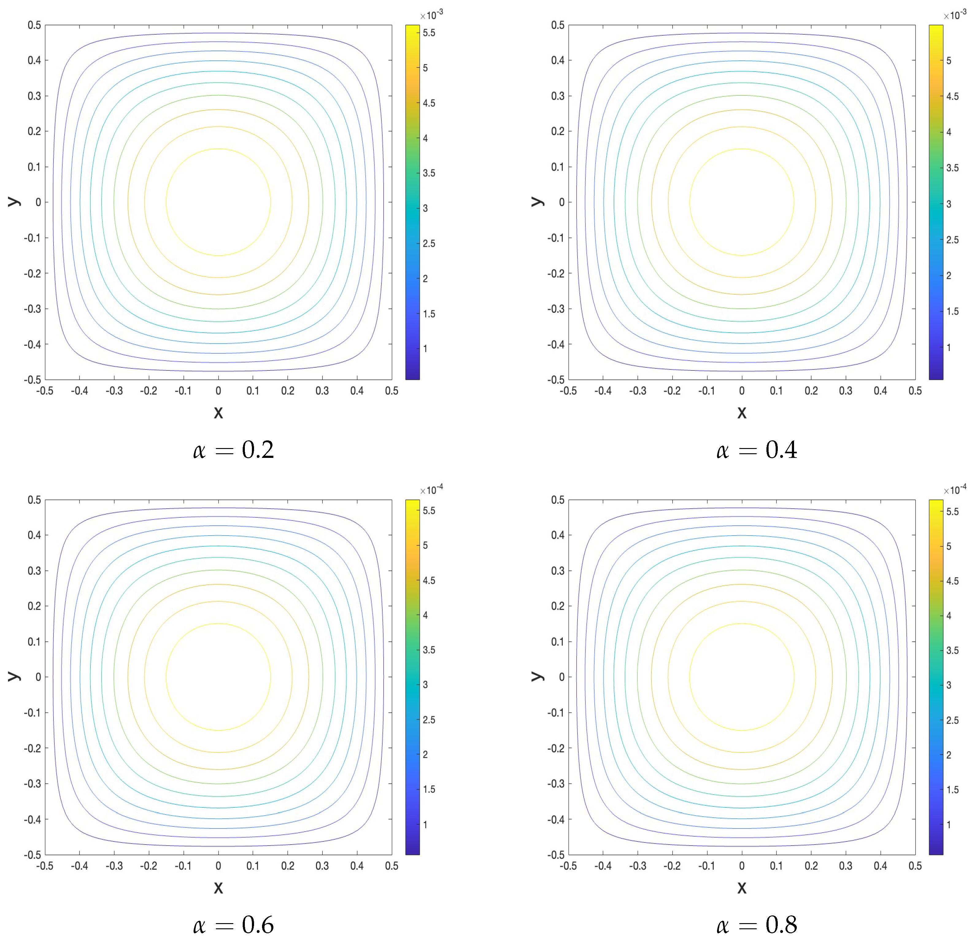
Figure 1 depicts a comparison of the numerical errors for $\alpha$ values of 0.2, 0.4, 0.6, and 0.8 when $M=N=100$.

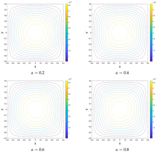
Figure 1. Contour plots of the numerical errors when $M=N=100$ for different values of $\alpha$.

Example 2. 

In this example, we consider the following 2D time-fractional nonlinear Schrödinger equation:

$$\begin{array}{c}i{\displaystyle \frac{{\partial }^{\alpha }u\left(x,y,t\right)}{\partial t^{\alpha }}}={\displaystyle \frac{{\partial }^{2}u\left(x,y,t\right)}{\partial x^2}}+{\displaystyle \frac{{\partial }^{2}u\left(x,y,t\right)}{\partial y^2}}+{\left|u\left(x,y,t\right)\right|}^{2}u\left(x,y,t\right)+f\left(x,y,t\right),\\ (x,y)\in \Omega =\left(0,1\right)\times \left(0,1\right),t\in \left(0,1\right],\\ f\left(x,y,t\right)=\left(1+i\right)\left(2t^2\left(x\left(1-x\right)+y\left(1-y\right)\right)+2{\left(\left(x-1\right)\left(y-1\right)xy{t}^2\right)}^3\right.\\ +\left.2ixy\left(x-1\right)\left(y-1\right){\displaystyle \frac{t^{2-\alpha }}{\Gamma \left(3-\alpha \right)}}\right).\end{array}$$

The initial and boundary values of the equation are given by the following exact solution:

$$u\left(x,y,t\right)=\left(1+i\right)\left(x-1\right)\left(y-1\right)xy{t}^2.$$

Table 3 shows the $L^{\infty }$-error and the convergence order in space, when h is reduced from h to ${\displaystyle \frac{h}{2}}$ and $\tau$ is reduced from $\tau$ to ${\displaystyle \frac{\tau }{2^{\frac{4}{1+\alpha }}}}$, respectively. The result shows that the difference scheme $\left(13\right)$ has fourth-order accuracy in a spatial direction for Example 2.

Table 3. Example 2: when $T=1$, computational errors and orders of convergence.

$\mathit{\alpha }$	h	N	${\mathit{L}}^{\mathit{\infty }}$-Error	Order
	1/5	100	$4.6778\times {10}^{-3}$	-
0.1	1/10	1243	$3.1551\times {10}^{-4}$	3.8901
	1/20	15457	$1.8410\times {10}^{-5}$	4.0091
	1/5	100	$6.7882\times {10}^{-4}$	-
0.5	1/10	635	$4.5434\times {10}^{-5}$	3.9012
	1/20	4031	$2.8172\times {10}^{-6}$	4.0114
	1/5	100	$1.3734\times {10}^{-4}$	-
0.9	1/10	430	$9.1009\times {10}^{-6}$	3.9156
	1/20	1850	$5.5536\times {10}^{-7}$	4.0345

From Table 4, it can be observed that the difference scheme (13) has $O\left({\tau }^{1+\alpha }\right)$ convergence accuracy in time, which shows the $L^{\infty }$-error and the convergence order in time with different values of $\alpha (0.25,0.5,0.75)$ when $M=100$ for Example 2.

Table 4. Example 2: when $T=1,M=100$, computational errors and orders of convergence.

$\mathit{\alpha }$	$\mathit{\tau }$	${\mathit{L}}^{\mathit{\infty }}$-Error	Order	CPU(s)
	1/20	$1.7278\times {10}^{-2}$	-	9.94
0.25	1/40	$7.4531\times {10}^{-3}$	1.2130	17.12
	1/80	$3.1501\times {10}^{-3}$	1.2424	33.43
	1/20	$7.9676\times {10}^{-3}$	-	9.05
0.5	1/40	$2.8518\times {10}^{-3}$	1.4823	16.98
	1/80	$1.0154\times {10}^{-3}$	1.4898	37.28
	1/20	$3.9413\times {10}^{-3}$	-	12.59
0.75	1/40	$1.1928\times {10}^{-3}$	1.7243	20.57
	1/80	$3.5950\times {10}^{-4}$	1.7303	34.23

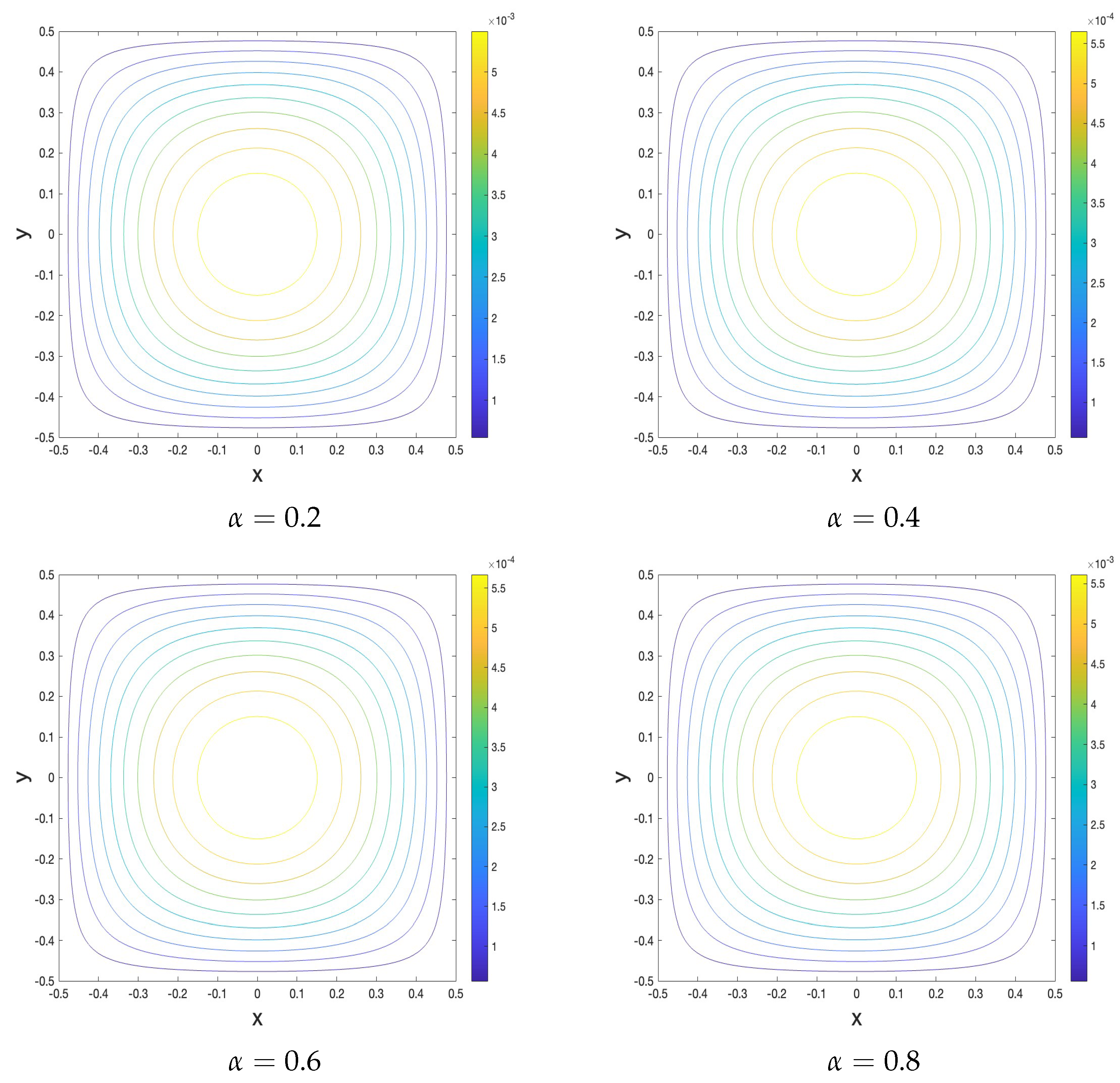
Figure 2 displays contour plots of the numerical errors for $\alpha$ with different values $0.2,0.4,0.6$, and 0.8 when $M=N=100$.

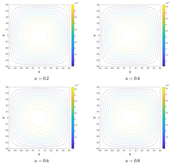
Figure 2. Contour plots of the numerical errors when $M=N=100$ for different values of $\alpha$.

6. Conclusions

In this article, we applied the $L1-2-3$ formula and the fourth-order compact difference formula to construct a linearized high-order compact difference scheme for the 2D time-fractional nonlinear Schrödinger equation with the well-known Caputo time-fractional derivative of order $\alpha$, the difference scheme (13) with convergence order $O({\tau }^{1+\alpha }+h_x^4+h_y^4)$. Similarity, we have proved that the unconditional stability and convergence of the compact difference scheme, and provide examples to illustrate the effectiveness of the difference scheme.

This paper provides two numerical experiments and compares the present compact ADI scheme with a difference scheme in [14]. The results of the numerical examples show that the difference scheme proposed in this paper is very effective at solving the two-dimensional time fractional nonlinear Schrödinger equation. In the future, we will consider some high-order exponential difference schemes [23] to improve the computational efficiency in time.

References

- Naber, M. Time fractional Schrödinger equation. J. Math. Phys. 2004, 45, 3339–3352. [Google Scholar] [CrossRef]
- Sun, Z.Z.; Zhang, Q.; Gao, G. Finite Difference Methods for Nonlinear Evolution Equations; Walter de Gruyter GmbH & Co. KG: Berlin, Germany, 2023. [Google Scholar]
- Gao, Z.; Xie, S. Fourth-order alternating direction implicit compact finite difference schemes for two-dimensional Schrödinger equations. Appl. Numer. Math. 2011, 61, 593–614. [Google Scholar] [CrossRef]
- Podlubny, I. Fractional Differential Equations; Academic Press: Cambridge, MA, USA, 1999. [Google Scholar]
- Gao, G.H.; Sun, Z.Z.; Zhang, H.W. A new fractional numerical differentiation formula to approximate the Caputo fractional derivative and its applications. J. Comput. Phys. 2014, 259, 33–50. [Google Scholar] [CrossRef]
- Alikhanov, A.A. A New Difference Scheme for the Time Fractional Diffusion Equation; Academic Press Professional, Inc.: Cambridge, MA, USA, 2015. [Google Scholar]
- Roul, P.; Rohil, V. A novel high-order numerical scheme and its analysis for the two-dimensional time-fractional reaction-subdiffusion equation. Numer. Algorithms 2022, 90, 1357–1387. [Google Scholar] [CrossRef]
- Wang, Y.M.; Ren, L. A high-order L2-compact difference method for Caputo-type time-fractional sub-diffusion equations with variable coefficients. Appl. Math. Comput. 2019, 342, 71–93. [Google Scholar] [CrossRef]
- Jin, C.; Zhizhong, S.; Hongwei, W. A high accurate and conservative difference scheme for the solution of nonlinear Schrödinger eqaution. Numer. Math. J. Chin. Univ. 2015, 37, 31–52. [Google Scholar]
- Rezamokhtari, G. Stability and Convergence Analyses of the FDM Based on Some L-Type Formulae for Solving the Subdiffusion Equation. Numer. Math. Theory Methods Appl. 2021, 14, 945. [Google Scholar]
- Dai, W.; Nassar, R. A New ADI Scheme for Solving Three-Dimensional Parabolic Equations with First-Order Derivatives and Variable Coefficients. J. Comput. Anal. Appl. 2000, 2, 293–308. [Google Scholar]
- Fei, M.; Wang, N.; Huang, C.; Ma, X. A second-order implicit difference scheme for the nonlinear time-space fractional Schrödinger equation. Appl. Numer. Math. 2020, 153, 399–411. [Google Scholar] [CrossRef]
- Wu, L.; Zhai, S. A new high order ADI numerical difference formula for time-fractional convection-diffusion equation. Appl. Math. Comput. 2019, 387, 124564. [Google Scholar] [CrossRef]
- Eskar, R.; Feng, X.; Kasim, E. On high-order compact schemes for the multidimensional time-fractional Schrödinger equation. Adv. Differ. Equ. 2020, 2020, 492. [Google Scholar] [CrossRef]
- Mokhtari, R.; Mostajeran, F. A high order formula to approximate the Caputo fractional derivative. Appl. Math. Comput. 2020, 2, 29. [Google Scholar] [CrossRef]
- Lin, Y.; Xu, C. Finite difference/spectral approximations for the time-fractional diffusion equation. J. Comput. Phys. 2007, 225, 1533–1552. [Google Scholar] [CrossRef]
- Holte, J.M. Discrete Gronwall lemma and applications. In Proceedings of the MAA-NCS Meeting at the University of North Dakota, Collegeville, MN, USA, 19–24 July 2009; Sciene Press: Beijing, China, 2021; 24, pp. 1–7. [Google Scholar]
- Zhang, Y.N.; Sun, Z.Z. Error Analysis of a Compact ADI Scheme for the 2D Fractional Subdiffusion Equation. J. Sci. Comput. 2014, 59, 104–128. [Google Scholar] [CrossRef]
- Wang, Y.M. Error and extrapolation of a compact LOD method for parabolic differential equations. J. Comput. Appl. Math. 2011, 235, 1367–1382. [Google Scholar] [CrossRef]
- Sun, Z.Z. Numerical Solution of Partial Differential Equations; Science Press: Beijing, China, 2005. [Google Scholar]
- Atouani, N.; Omrani, K. On the convergence of conservative difference schemes for the 2D generalized Rosenau–Korteweg de Vries equation. Appl. Math. Comput. 2015, 250, 832–847. [Google Scholar] [CrossRef]
- Liao, H.L.; Sun, Z.Z. Maximum norm error bounds of ADI and compact ADI methods for solving parabolic equations. Numer. Methods Partial Differ. Equ. 2010, 26, 37–60. [Google Scholar] [CrossRef]
- Bhatt, H.P.; Khaliq, A.Q.M. Higher order exponential time differencing scheme for system of coupled nonlinear Schrdinger equations. Appl. Math. Comput. 2014, 228, 271–291. [Google Scholar]
Disclaimer/Publisher’s Note: The statements, opinions and data contained in all publications are solely those of the individual author(s) and contributor(s) and not of MDPI and/or the editor(s). MDPI and/or the editor(s) disclaim responsibility for any injury to people or property resulting from any ideas, methods, instructions or products referred to in the content. |
© 2024 by the authors. Licensee MDPI, Basel, Switzerland. This article is an open access article distributed under the terms and conditions of the Creative Commons Attribution (CC BY) license (https://creativecommons.org/licenses/by/4.0/).