Article

Bifurcation Analysis and Chaos Control of a Discrete Fractional-Order Modified Leslie–Gower Model with Nonlinear Harvesting Effects

1
School of Mathematics and Physics, Hebei University of Engineering, Handan 056038, China
2
School of Mathematics and Statistics, Shandong University Weihai, Weihai 264209, China
3
Department of Mathematics, Harbin Institute of Technology Weihai, Weihai 264209, China
*
Author to whom correspondence should be addressed.
Fractal Fract. 2024, 8(12), 744; https://doi.org/10.3390/fractalfract8120744
Submission received: 8 November 2024 / Revised: 29 November 2024 / Accepted: 14 December 2024 / Published: 16 December 2024

Abstract

:
This paper investigates the dynamical behavior of a discrete fractional-order modified Leslie–Gower model with a Michaelis–Menten-type harvesting mechanism and a Holling-II functional response. We analyze the existence and stability of the nonnegative equilibrium points. For the interior equilibrium points, we study the conditions for period-doubling and Neimark–Sacker bifurcations using the center manifold theorem and bifurcation theory. To control the chaos arising from these bifurcations, two chaos control strategies are proposed. Numerical simulations are performed to validate the theoretical results. The findings provide valuable insights into the sustainable management and conservation of ecological systems.

1. Introduction

1.1. Motivation and Literature Review

The interactions between prey and predator populations have long been a central focus in mathematical ecology. In 1910, Lotka [1] proposed a prey–predator model resembling a chemical reaction, followed by Volterra [2,3], who explored similar dynamics in 1926. Later, Holling [4,5] expanded the model to include density-dependent prey growth and various functional responses. The Leslie–Gower model [6,7], another key framework in prey–predator studies, was subsequently modified by May [8].
In [9], Gupta and Chandra proposed a modified Leslie–Gower model that incorporates the Holling-II functional response and a Michaelis–Menten-type prey harvesting effect. The model is expressed as follows:
d X d T = r X 1 X K a 1 X Y n + X q E X m 1 E + m 2 X , d Y d T = s Y 1 a 2 Y n + X ,
with initial conditions X ( 0 ) 0 and Y ( 0 ) 0 . Here, all parameters are positive, and a concise description of each parameter, emphasizing its biological significance, is provided in Table 1. In [10], Hu and Cao examined the existence and stability of possible equilibrium points within the system, identifying saddle-node, transcritical, Hopf, and Bogdanov–Takens bifurcations at these points. Song et al. [11] provided rigorous results regarding the Hopf bifurcation properties in a diffusive predator–prey system. Chen et al. [12] explored a discrete-time prey–predator model featuring Michaelis–Menten-type harvesting, and exhibited Fold, Flip, and Neimark–Sacker bifurcations under specific conditions. Numerous additional studies have contributed to this model; for more information, see [13,14,15] and their references.
Here, we adopt a parameter scaling approach as outlined in a previous study [16], implementing the following transformations:
t = r T , x = X K , y = a 1 Y K , ω = 1 r , β = a 2 a 1 , k = n K , σ = q E r m 2 K , m = m 1 E m 2 K , γ = s r .
The system in (1) is then transformed into
d x d t = x 1 x ω x y k + x σ x m + x , d y d t = γ y 1 β y k + x ,
with the initial conditions x ( 0 ) = x 0 0 and y ( 0 ) = y 0 0 .
Considering that the responses between biological populations often have delay effects, integer-order derivative models can only describe instantaneous changes and fail to capture the variations from previous moments. Therefore, we further investigate fractional-order derivative models, as they can better account for past dynamics and more effectively simulate the interactions between organisms in real-world environments. Moustafa et al. [17] proposed and analyzed a fractional-order eco-epidemiological model with the disease affecting the prey species, demonstrating the non-negativity and boundedness of the model’s solutions. Arif et al. [18] examined a fractional-order system modeling a predator and two prey populations, utilizing the Caputo fractional derivative. They determined the equilibrium points of this system and assessed its stability. Wang and Li [19] investigated a fractional-order predator–prey model incorporating anti-predator behavior and a Holling-IV functional response. They analyzed the local asymptotic stability, period-doubling bifurcation, and Neimark–Sacker bifurcation of the discretized version of the model. Mua et al. [20] investigated the dynamics and feedback control tactics of a discrete predator–prey competitive model. For additional findings on this topic, readers can consult [21,22,23,24,25,26] and their references. Inspired by this idea, we seek to extend Equation (2) into a fractional-order model by incorporating the left conformable fractional derivative [27,28]. The left conformable fractional derivative is defined as follows:
Definition 1.
Let f : [ h , ) R be a function. The left conformable fractional derivative of f ( t ) at t > h of order 0 < α 1 is defined as
T h α f ( t ) = lim ε 0 f ( t + ε ( t h ) 1 α ) f ( t ) ε .
When h = 0 , the left conformable fractional derivative T h α is equal to the conformable fractional derivative T α . It is shown in [28] that the following result holds:
T h α f ( t ) = ( t h ) 1 α f ( t ) .
Note that when calculating the left conformable fractional derivative of a function f ( t ) , both the fractional order α and the starting point h are fixed parameters, while t is the variable that changes. To highlight the dependence of the derivative on both α and h, we adopt the notation T h α , which explicitly reflects this relationship. It is important to emphasize that this notation does not suggest that the derivative operation itself is multi-valued.
By substituting the integer-order derivative in model (2) with the left conformable fractional derivative, we obtain the following fractional-order model:
T α x = x 1 x ω x y k + x σ x m + x , T α y = γ y 1 β y k + x .
where the fractional-order parameter α ( 0 , 1 ] . In particular, when α = 1 , the fractional-order model (3) reduces to the classical integer-order model (2), demonstrating that the fractional-order model serves as a generalization of the integer-order model. Moreover, in fractional calculus, the rate of change at any given time, as described by the fractional-order derivative, is not solely dependent on the current state but also on the population dynamics over a preceding time interval. This inherent feature endows the fractional-order model (3) with the capacity to capture memory effects, thereby providing a more nuanced representation of population dynamics that accounts for past influences.

1.2. Discrete Fractional-Order Modified Leslie–Gower Model with Harvesting

In practice, biological sample data are typically collected at discrete intervals, such as weekly or monthly, rather than on a continuous basis. Consequently, discrete models often provide greater accuracy compared to continuous models. Moreover, discrete models are particularly appropriate for populations that exhibit non-overlapping generation characteristics or small sizes [29]. Therefore, using discrete models to study the dynamic behavior of biological populations holds considerable practical significance. In previous studies, such as Shi et al. [16,30], researchers applied the piecewise constant approximation technique to discretize continuous fractional-order predator–prey models, thoroughly analyzing the associated dynamical behaviors. Singh and Sharma [31] focused on a discrete predator–prey model with a Holling type II functional response, incorporating prey refuges, and investigated bifurcation phenomena, as well as chaos control strategies through state feedback, pole placement, and hybrid methods. In another study, Berkal and Almatrafi [32] employed an exponential piecewise constant approximation to discretize a continuous fractional-order activator–inhibitor system. Their analysis included stability evaluations, an exploration of Neimark–Sacker and period-doubling bifurcations, and numerical simulations, which corroborated the theoretical results on the system’s dynamics. For additional insights into the field of discrete population models, readers are encouraged to refer to works such as [19,33,34,35] and other related references. However, to date, there has been a noticeable gap in the literature concerning fractional discrete-time Leslie–Gower predator–prey models, particularly those that integrate nonlinear harvesting mechanisms in the prey population.
Next, we apply the piecewise constant argument approach [36] to derive the discretized version of model (3). Since x ( t ) > 0 and y ( t ) > 0 , model (3) can be expressed as follows:
T α x x = 1 x ω y k + x σ m + x , T α y y = γ 1 β y k + x .
Using the piecewise constant argument approach, model (4) transforms into
T α x ( t ) x ( t ) = 1 x t h h ω y t h h k + x t h h σ m + x t h h , T α y ( t ) y ( t ) = γ 1 β y t h h k + x t h h ,
where t h denotes the integer part of t [ n h , ( n + 1 ) h ) , n = 0 , 1 , . And h > 0 is a discretization parameter that represents the time interval for production. Applying Definition 1 to the first equation of model (5), we obtain
( t n h ) 1 α d x ( t ) x ( t ) d t = 1 x ( n h ) ω y ( n h ) k + x ( n h ) σ m + x ( n h ) .
Integrating this equation over the interval [ n h , t ) leads to
ln ( x ( t ) ) ln ( x ( n h ) ) = 1 x ( n h ) ω y ( n h ) k + x ( n h ) σ m + x ( n h ) ( t n h ) α α .
Letting t ( n + 1 ) h and replacing x ( n h ) and y ( n h ) by x n and y n , respectively, we have
x n + 1 = x n e h α α 1 x n ω y n k + x n σ m + x n .
The second equation of model (5) is solved in a similar manner, resulting in
y n + 1 = y n e h α α γ 1 β y n k + x n .
Thus, the discrete version of the model (3) is presented as follows:
x n + 1 = x n e h α α 1 x n ω y n k + x n σ m + x n , y n + 1 = y n e h α α γ 1 β y n k + x n .

1.3. Main Contributions

This paper aims to explore the dynamical properties of model (6). The main contributions of this study are as follows:
Establishing conditions for the existence and stability of nonnegative equilibrium points in model (6);
Identifying bifurcation sets and conducting a comprehensive analysis of the interior equilibrium point;
Employing state feedback control and hybrid control methodologies to manage bifurcations and chaos in model (6);
Validating our theoretical findings through numerical simulations using MATLAB and Mathematica.

1.4. Structure of the Paper

This paper is organized as follows: Section 2 determines the nonnegative equilibrium points of model (6) and analyzes their stability. Section 3 derives the sufficient conditions for period-doubling and Neimark–Sacker bifurcations and examines the stability of the resulting orbits using the center manifold theorem and bifurcation theory. In Section 4, we apply state feedback and hybrid control strategies to control chaos in model (6). Section 5 presents numerical simulations to validate the key analytical results. The paper concludes with a summary of the findings and recommendations for future research in the final section.

2. Existence and Stability of Nonnegative Equilibrium Points

2.1. Existence of Nonnegative Equilibrium Points

To identify the nonnegative equilibrium points, we must solve the following system:
x = x e h α α 1 x ω y k + x σ m + x , y = y e h α α γ 1 β y k + x .
We begin by examining the boundary equilibrium points, corresponding to the cases where either x = 0 or y = 0 . When x = 0 , the model (6) yields two boundary equilibrium points: B 0 = ( 0 , 0 ) and B y = 0 , k β . For y = 0 , substituting into (7) leads to the equation for x:
x 2 + ( m 1 ) x + σ m = 0 .
as shown in Equation (8). A necessary condition for the existence of boundary equilibrium points is that ( m + 1 ) 2 4 σ . In this case, the roots of (8) can be expressed as
x 1 = 1 m + ( m + 1 ) 2 4 σ 2 , x 2 = 1 m ( m + 1 ) 2 4 σ 2 ,
Specifically, when ( m + 1 ) 2 = 4 σ , the roots x 1 and x 2 collide, which we denote as
x 3 = 1 m 2 .
Considering the biological significance of model (6), we focus on its positive solutions to equation (8). Consequently, we can readily summarize the following findings regarding the existence of boundary equilibrium points for model (6).
Theorem 1.
The model (6) consistently exhibits two boundary equilibrium points: B 0 = ( 0 , 0 ) and B y = 0 , k β . For the existence of additional boundary equilibrium points, the following conditions are established:
(1) 
If m < σ , m < 1 , and ( m + 1 ) 2 > 4 σ , two distinct boundary equilibrium points, B x 1 = ( x 1 , 0 ) and B x 2 = ( x 2 , 0 ) , exist;
(2) 
If m < 1 and ( m + 1 ) 2 = 4 σ , only one boundary equilibrium point, B x 3 = ( x 3 , 0 ) , exists;
(3) 
If either m = σ < 1 or m > σ , a single boundary equilibrium point, B x 1 = ( x 1 , 0 ) , exists.
The values of x 1 , x 2 , and x 3 are given by Equations (9) and (10), respectively.
Next, we examine the interior equilibrium points, which satisfy the system of equations:
1 x ω y k + x σ m + x = 0 , 1 β y k + x = 0 .
Substituting y = k + x β into the first equation of (11) leads to the quadratic equation:
β x 2 + [ ω + ( m 1 ) β ] x + m ω + ( σ m ) β = 0 .
Let Δ denote the discriminant of this quadratic equation, defined as
Δ = [ ω + ( m 1 ) β ] 2 4 β [ m ω + ( σ m ) β ] = [ ω ( m + 1 ) β ] 2 4 σ β 2 .
The condition for real solutions is Δ 0 . When Δ > 0 , the Equation (12) has two distinct solutions:
x 1 * = ω ( m 1 ) β + Δ 2 β , x 2 * = ω ( m 1 ) β Δ 2 β ,
and when Δ = 0 , there is a unique solution:
x 3 * = ω ( m 1 ) β 2 β .
Thus, the existence of interior equilibrium points of model (6) is determined by the conditions summarized below.
Theorem 2.
The following conditions characterize the interior equilibrium points of model (6):
(1) 
If m ω > ( m σ ) β , ω < ( 1 m ) β , and [ ω ( m + 1 ) β ] 2 > 4 σ β 2 , then there are two distinct interior equilibrium points, E 1 = ( x 1 * , y 1 * ) and E 2 = ( x 2 * , y 2 * ) ;
(2) 
If ω < ( 1 m ) β and [ ω ( m + 1 ) β ] 2 = 4 σ β 2 , then there is only one interior equilibrium point, E 3 = ( x 3 * , y 3 * ) ;
(3) 
If either ( m σ ) β m = ω < ( 1 m ) β or m ω < ( m σ ) β , then there is only one interior equilibrium point, E 1 = ( x 1 * , y 1 * ) .
Here, x i * are given by (13) or (14), and y i * = k + x i * β for i = 1 , 2 , 3 .

2.2. Stability of Nonnegative Equilibrium Points

We denote the Jacobian matrix evaluated at the equilibrium point ( x , y ) as follows:
J ( ( x , y ) ) = J 11 J 12 J 21 J 22
where
J 11 = 1 + h α x α 1 + ω y ( k + x ) 2 + σ ( m + x ) 2 e h α α 1 x ω y k + x σ m + x , J 12 = h α ω x α ( k + x ) e h α α 1 x ω y k + x σ m + x , J 21 = h α γ β y 2 α ( k + x ) 2 e h α α γ 1 β y k + x , J 22 = 1 h α y γ β α ( k + x ) e h α α γ 1 β y k + x .
The characteristic equation of J ( E ) is expressed as F ( λ ) = λ 2 M λ + N = 0 , where λ 1 and λ 2 are its roots. To analyze the stability of these equilibrium points, we first present the following definition and lemma.
Definition 2
([37,38]). The classification of the equilibrium point ( x , y ) is as follows:
(1) 
If | λ 1 |   < 1 and | λ 2 |   < 1 , the equilibrium point exhibits a sink-point behavior and is locally asymptotically stable;
(2) 
If | λ 1 |   > 1 and | λ 2 |   > 1 , the equilibrium point exhibits a source-point behavior and is locally unstable;
(3) 
If | λ 1 |   > 1 and | λ 2 |   < 1 (or | λ 1 |   < 1 and | λ 2 |   > 1 ), the equilibrium point exhibits a saddle-point behavior;
(4) 
If either | λ 1 |   = 1 or | λ 2 |   = 1 , the equilibrium point exhibits a non-hyperbolic-point behavior.
Lemma 1
([37,38]). The following statements are applicable to the roots of the characteristic equation F ( λ ) = λ 2 M λ + N = 0 .
(1) 
If F ( 1 ) > 0 , then
(a) 
| λ 1 |   < 1 and | λ 2 |   < 1 if and only if F ( 1 ) > 0 and F ( 0 ) < 1 ;
(b) 
| λ 1 |   < 1 and | λ 2 |   > 1 (or | λ 1 |   > 1 and | λ 2 |   < 1 ) if and only if F ( 1 ) < 0 ;
(c) 
| λ 1 |   > 1 and | λ 2 |   > 1 if and only if F ( 1 ) > 0 and F ( 0 ) > 1 ;
(d) 
λ 1 = 1 and | λ 2 |   1 if and only if F ( 1 ) = 0 and M 0 , 2 ;
(e) 
λ 1 and λ 2 are a pair of conjugate complex roots and | λ 1 , 2 |   = 1 if and only if M 2 < 4 N and F ( 0 ) = 1 .
(2) 
If F ( 1 ) = 0 , then one of the roots satisfies λ 1 = 1 . Furthermore, the other root | λ 2 |   < 1 (or | λ 2 |   = 1 or | λ 2 |   > 1 ) holds if and only if | F ( 0 ) | < 1 (or | F ( 0 ) | = 1 or | F ( 0 ) | > 1 ).
(3) 
If F ( 1 ) < 0 , then one root satisfies λ 1 ( 1 , ) , which implies | λ 1 |   > 1 . Furthermore, the other root
(a) 
| λ 2 |   > 1 if and only if F ( 1 ) < 0 ;
(b) 
| λ 2 |   < 1 if and only if F ( 1 ) > 0 ;
(c) 
λ 2 = 1 if and only if F ( 1 ) = 0 .
From Equation (15), we can derive the Jacobian matrices at the boundary equilibrium points B 0 and B y as follows:
J ( B 0 ) = e h α α 1 σ m 0 0 e h α α γ ,
J ( B y ) = e h α α 1 ω β σ m 0 h α γ α β 1 h α γ α .
Thus, the eigenvalues of B 0 are λ 1 = e h α α 1 σ m and λ 2 = e h α α γ > 1 . When σ < m , λ 1 < 1 , and based on Definition 2(2), we conclude that the equilibrium point B 0 exhibits a source-point behavior. When σ > m , λ 1 > 1 , and based on Definition 2(3), we conclude that B 0 exhibits a saddle-point behavior. When σ = m , λ 1 = 1 , and based on Definition 2(4), we conclude that B 0 exhibits a non-hyperbolic-point behavior. Similarly, the local stability of B y can be deduced, leading to the following theorem.
Theorem 3.
The subsequent statements hold for the boundary equilibrium points B 0 and B y .
(1) 
The point B 0 ( 0 , 0 ) exhibits the following behaviors:
(a) 
The equilibrium point B 0 ( 0 , 0 ) exhibits a source-point behavior if σ < m ;
(b) 
The equilibrium point B 0 ( 0 , 0 ) exhibits a saddle-point behavior if σ > m ;
(c) 
The equilibrium point B 0 ( 0 , 0 ) exhibits a non-hyperbolic-point behavior if σ = m .
(2) 
The point B y ( 0 , k β ) exhibits the following behaviors:
(a) 
The equilibrium point B y ( 0 , k β ) exhibits a sink-point behavior if ω β + σ m > 1 and h α γ < 2 α ;
(b) 
The equilibrium point B y ( 0 , k β ) exhibits a source-point behavior if ω β + σ m < 1 and h α γ > 2 α ;
(c) 
The equilibrium point B y ( 0 , k β ) exhibits a non-hyperbolic-point behavior if ω β + σ m = 1 or h α γ = 2 α ;
(d) 
The equilibrium point B y ( 0 , k β ) exhibits a saddle-point behavior under other conditions.
Similarly, we can use Definition 2 to conduct a systematic stability analysis of the remaining boundary equilibrium points.
Theorem 4.
Under the conditions of the existence of boundary equilibrium points of model (6) in Theorem 1:
(1) 
The point B x 1 exhibits the following behaviors:
(a) 
The equilibrium point B x 1 exhibits a saddle-point behavior if h α α < 2 ( m + x 1 ) x 1 ( m + 1 ) 2 4 σ ;
(b) 
The equilibrium point B x 1 exhibits a source-point behavior if h α α > 2 ( m + x 1 ) x 1 ( m + 1 ) 2 4 σ ;
(c) 
The equilibrium point B x 1 exhibits a non-hyperbolic-point behavior if h α α = 2 ( m + x 1 ) x 1 ( m + 1 ) 2 4 σ .
(2) 
The point B x 2 always exhibits a source-point behavior and is unstable.
(3) 
The point B x 3 always exhibits a non-hyperbolic-point behavior.
Proof. 
At the boundary equilibrium points B x i ( i = 1 , 2 , 3 ) , we have 1 x i = σ m + x i . The Jacobian matrix can be expressed as
J ( B x i ) = 1 + h α x i α 1 + σ ( m + x i ) 2 h α ω x i α ( k + x i ) 0 e h α α γ , i = 1 , 2 , 3 .
Thus, the eigenvalues of J ( B x i ) are λ 1 = 1 + h α x i α 1 + σ ( m + x i ) 2 and λ 2 = e h α α γ > 1 .
(1)
For x 1 = 1 m + ( m + 1 ) 2 4 σ 2 , we can obtain
( m + x 1 ) 2 σ = 1 4 1 + m + ( m + 1 ) 2 4 σ 2 σ = 1 4 2 ( m + 1 ) 2 + 2 ( m + 1 ) ( m + 1 ) 2 4 σ 4 σ σ = ( m + 1 ) 2 4 σ 2 ( m + 1 ) 2 4 σ + 1 + m > 0 ,
which implies
λ 1 = 1 + h α x 1 α 1 + σ ( m + x 1 ) 2 = 1 + h α x 1 α σ ( m + x 1 ) 2 ( m + x 1 ) 2 < 1 .
Additionally, since x 1 satisfies 1 x 1 σ m + x 1 = 0 , we have
h α x 1 α 1 + σ ( m + x 1 ) 2 = h α x 1 α 1 + 1 x 1 m + x 1 = h α x 1 α ( m + 1 ) 2 4 σ m + x 1
Therefore, if h α α < 2 ( m + x 1 ) x 1 ( m + 1 ) 2 4 σ holds, then | λ 1 |   < 1 , indicating that B x 1 is a saddle point. This completes the proof for part (a). The proofs for parts (b) and (c) follow similarly.
(2)
For x 2 = 1 m ( m + 1 ) 2 4 σ 2 , we find that
( m + x 2 ) 2 σ = 1 4 1 + m ( m + 1 ) 2 4 σ 2 σ = 1 4 2 ( m + 1 ) 2 2 ( m + 1 ) ( m + 1 ) 2 4 σ 4 σ σ = ( m + 1 ) 2 4 σ 2 ( m + 1 ) 2 4 σ ( 1 + m ) < 0 .
Consequently, we deduce that λ 1 > 1 . According to Definition 2, B x 2 is a source and it is unstable when it exists.
(3)
For x 3 = 1 m 2 , from ( m + 1 ) 2 4 σ = 0 , we can conclude that ( m + x 3 ) 2 = σ . Therefore, the eigenvalues of J ( B x 3 ) are λ 1 = 1 and λ 2 > 1 , indicating that B x 3 is always classified as non-hyperbolic according to Definition 2.
This completes the proof. □
Next, we analyze the stability of the interior equilibrium points E i ( x i * , y i * ) , i = 1 , 2 , 3 . The characteristic equation of the Jacobian matrix J ( E i ) is
F ( λ ) λ 2 ( A M + 2 ) λ + A 2 N + A M + 1 = 0 ,
where
A = h α α , M = x i * 1 + ω β ( k + x i * ) + σ ( m + x i * ) 2 γ , N = x i * γ 1 σ ( m + x i * ) 2 .
Thus,
F ( 1 ) = A 2 N , F ( 1 ) = A 2 N + 2 A M + 4 .
We use Definition 2 and Lemma 1 to investigate the stability of each interior equilibrium point.
Theorem 5.
Suppose that one of the following three conditions is satisfied:
(i) 
m ω > ( m σ ) β , ω < ( 1 m ) β , and [ ω ( m + 1 ) β ] 2 > 4 σ β 2 ;
(ii) 
( m σ ) β m = ω < ( 1 m ) β ;
(iii) 
m ω < ( m σ ) β .
Then, the interior equilibrium point E 1 of model (6) exhibits the following behaviors:
(1) 
The interior equilibrium point E 1 exhibits a sink-point behavior if one of the following conditions holds:
(a) 
M 2 4 N and 0 < A < M M 2 4 N N ;
(b) 
M 2 < 4 N and 0 < A < M N .
(2) 
The interior equilibrium point E 1 exhibits a saddle-point behavior if M 2 4 N and M M 2 4 N N < A < M + M 2 4 N N .
(3) 
The interior equilibrium point E 1 exhibits a source-point behavior if one of the following conditions holds:
(a) 
M 2 4 N and A > M + M 2 4 N N ;
(b) 
M 2 < 4 N and A > M N .
(4) 
The interior equilibrium point E 1 exhibits a non-hyperbolic-point behavior if one of the following conditions holds:
(a) 
M 2 4 N and A = M ± M 2 4 N N ;
(b) 
M 2 < 4 N and A = M N .
Proof. 
We start by determining the sign of F ( 1 ) = A 2 N , which depends on the sign of N. Since E 1 ( x 1 * , y 1 * ) satisfies (11) and x 1 * = ω ( m 1 ) β + Δ 2 β , we deduce that
N x 1 * = x 1 * γ 1 σ ( m + x 1 * ) 2 = x 1 * γ 1 1 m + x 1 * 1 x 1 * ω β = x 1 * γ m + x 1 * 2 x 1 * + m 1 + ω β = x 1 * γ Δ β ( m + x 2 * ) > 0 .
Thus, it follows that F ( 1 ) > 0 .
Next, we consider F ( 1 ) = A 2 N + 2 A M + 4 . When M 2 4 N , the equation F ( 1 ) = 0 becomes a quadratic equation in terms of A with two solutions given by
A = M ± M 2 4 N N .
If
0 < A < M M 2 4 N N , o r A > M + M 2 4 N N ,
then F ( 1 ) > 0 . Conversely, when M 2 < 4 N , it follows directly that F ( 1 ) > 0 .
Finally, we examine the equation F ( 0 ) = A 2 N + A M + 1 . Since N ( x 1 * ) > 0 , we conclude that F ( 0 ) < 1 holds under the condition A < M N .
In summary, the conclusion for case (1) follows directly from the application of Lemma 1(1)(a). Cases (2)–(4) can be established in a similar manner by applying Lemma 1(1)(b)–(e), respectively. □
For the interior equilibrium point E 2 ( x 2 * , y 2 * ) , a calculation analogous to that for N ( x 1 * ) yields
N x 2 * = x 2 * γ Δ β ( m + x 2 * ) < 0 ,
which implies that F ( 1 ) < 0 . With the aid of Lemma 1, the following theorem can be readily established.
Theorem 6.
Suppose that m ω > ( m σ ) β , ω < ( 1 m ) β , and [ ω ( m + 1 ) β ] 2 > 4 σ β 2 . Then, the interior equilibrium point E 2 of model (6) satisfies the following:
(1) 
The interior equilibrium point E 2 exhibits a saddle-point behavior if 0 < A < M + M 2 4 N N ;
(2) 
The interior equilibrium point E 2 exhibits a source-point behavior if A > M + M 2 4 N N ;
(3) 
The interior equilibrium point E 2 exhibits a non-hyperbolic-point behavior if A = M + M 2 4 N N .
For the interior equilibrium point E 3 ( x 3 * , y 3 * ) , a calculation analogous to N ( x 1 * ) results in N ( x 3 * ) = 0 , thereby implying F ( 1 ) = 0 .
Theorem 7.
When [ ω ( m + 1 ) β ] 2 = 4 σ β 2 and ω < ( 1 m ) β , the interior equilibrium point E 3 of model (6) always exhibits non-hyperbolic-point behavior.

3. Bifurcation Analysis

In this section, we examine the bifurcation behavior near the equilibrium points of the model (6). We exclude an analysis of boundary equilibrium points corresponding to the extinction of either the predator or prey, which results in a single surviving population. Since the bifurcation analysis at the interior equilibrium points E i follows a similar procedure, we focus specifically on the local bifurcation behavior at the interior equilibrium point E 1 , taking h as the bifurcation parameter.

3.1. Period-Doubling Bifurcation

If a period-doubling bifurcation occurs at the equilibrium point, the stability of that point changes. Specifically, an initially stable equilibrium point can become unstable, leading to the emergence of new periodic orbits, typically with a period twice that of the original orbit. For such a bifurcation, the eigenvalues λ 1 , 2 of the Jacobian matrix J ( x 1 * , y 1 * ) must satisfy λ 1 = 1 and | λ 2 |   1 . This condition implies that
A M + 2 2 4 A 2 N + A M + 1 ,
h = h 1 : = α M M 2 4 N N 1 α , or h = h 2 : = α M + M 2 4 N N 1 α ,
and
h 2 α M 1 α , and h 4 α M 1 α .
These conditions indicate that a period-doubling bifurcation may occur at the interior equilibrium point E 1 when the parameters satisfy Equations (17)–(19). In this work, we focus on the case h = h 1 and omit the corresponding analysis for h = h 2 , as the reasoning is similar.
First, let u n = x n x 1 * and v n = y n y 1 * , which transforms the equilibrium point E 1 ( x 1 * , y 1 * ) to the origin O ( 0 , 0 ) , and model (6) is changed to
u n + 1 = ( u n + x 1 * ) e h α α 1 ( u n + x 1 * ) ω ( v n + y 1 * ) k + u n + x 1 * σ m + u n + x 1 * x 1 * , v n + 1 = ( v n + y 1 * ) e h α α γ 1 β ( v n + y 1 * ) k + u n + x 1 * y 1 * .
Second, given a small perturbation h * of the parameter h around the critical value h 1 , i.e., h * = h h 1 with 0 < h * 1 , then model (20) is perturbed into
u n + 1 = ( u n + x 1 * ) e ( h 1 + h * ) α α 1 ( u n + x 1 * ) ω ( v n + y 1 * ) k + u n + x 1 * σ m + u n + x 1 * x 1 * , v n + 1 = ( v n + y 1 * ) e ( h 1 + h * ) α α γ 1 β ( v n + y 1 * ) k + u n + x 1 * y 1 * .
Letting h n + 1 * = h n * = h * , model (21) becomes
u n + 1 = ( u n + x 1 * ) e ( h 1 + h n * ) α α 1 ( u n + x 1 * ) ω ( v n + y 1 * ) k + u n + x 1 * σ m + u n + x 1 * x 1 * , v n + 1 = ( v n + y 1 * ) e ( h 1 + h n * ) α α γ 1 β ( v n + y 1 * ) k + u n + x 1 * y 1 * , h n + 1 * = h n * .
Using the Taylor expansion of model (22) at ( u n , v n , h n * ) = ( 0 , 0 , 0 ) to the third order yields
u n + 1 v n + 1 h n + 1 * = a 11 a 12 0 a 21 a 22 0 0 0 1 u n v n h n * + f ( u n , v n , h n * ) + O ( ρ 1 3 ) g ( u n , v n , h n * ) + O ( ρ 1 3 ) 0 ,
where ρ 1 = u n 2 + v n 2 + ( h n * ) 2 ,
f ( u n , v n , h n * ) = a 13 u n 2 + a 14 u n v n + a 15 v n 2 + a 16 u n 3 + a 17 u n 2 v n + a 18 u n v n 2 + a 19 v n 3 + b 11 u n h n * + b 12 v n h n * + b 13 ( h n * ) 2 + b 14 u n 2 h n * + b 15 v n 2 h n * + b 16 u n v n h n * + b 17 ( h n * ) 3 + b 18 u n ( h n * ) 2 + b 19 v n ( h n * ) 2 , g ( u n , v n , h n * ) = a 23 u n 2 + a 24 u n v n + a 25 v n 2 + a 26 u n 3 + a 27 u n 2 v n + a 28 u n v n 2 + a 29 v n 3 + b 21 u n h n * + b 22 v n h n * + b 23 ( h n * ) 2 + b 24 u n 2 h n * + b 25 v n 2 h n * + b 26 u n v n h n * + b 27 ( h n * ) 3 + b 28 u n ( h n * ) 2 + b 29 v n ( h n * ) 2 ,
and the calculated values of a 11 , ⋯, a 19 , b 11 , ⋯, b 19 , a 21 , ⋯, a 29 , b 11 , ⋯, and b 29 are given in Appendix A.
Therefore, we obtain the Jacobian matrix of model (6) at the equilibrium point E 1 .
J ( E 1 ) = a 11 a 12 0 a 21 a 22 0 0 0 1 ,
and its eigenvalues
λ 1 = 1 , λ 2 = A M + 3 , λ 3 = 1 ,
with corresponding eigenvectors
( ξ 1 , ζ 1 , η 1 ) T = ( a 12 , 1 a 11 , 0 ) T , ( ξ 2 , ζ 2 , η 2 ) T = ( a 12 , λ 2 a 11 , 0 ) T , ( ξ 3 , ζ 3 , η 3 ) T = ( 0 , 0 , 1 ) T ,
respectively. Set
T 1 = a 12 a 12 0 1 a 11 λ 2 a 11 0 0 0 1 ,
then
T 1 1 = 1 a 12 ( 1 + λ 2 ) λ 2 a 11 a 12 0 1 + a 11 a 12 0 0 0 a 12 ( 1 + λ 2 ) .
Taking the transformation ( u n , v n , h n * ) T = T 1 ( p n , q n , w n ) T , then model (23) is changed into the following form:
p n + 1 = p n + f 1 ( p n , q n , w n ) + O ( ρ 2 3 ) , q n + 1 = λ 2 q n + g 1 ( p n , q n , w n ) + O ( ρ 2 3 ) , w n + 1 = w n ,
where ρ 2 = p n 2 + q n 2 + w n 2 ,
f 1 ( p n , q n , w n ) = I 13 u n 2 + I 14 u n v n + I 15 v n 2 + I 16 u n 3 + I 17 u n 2 v n + I 18 u n v n 2 + I 19 v n 3 + I 21 u n w n + I 22 v n w n + I 23 w n 2 + I 24 u n 2 w n + I 25 v n 2 w n + I 26 u n v n w n + I 27 w n 3 + I 28 u n w n 2 + I 29 v n w n 2 , g 1 ( p n , q n , w n ) = J 13 u n 2 + J 14 u n v n + J 15 v n 2 + J 16 u n 3 + J 17 u n 2 v n + J 18 u n v n 2 + J 19 v n 3 + J 21 u n w n + J 22 v n w n + J 23 w n 2 + J 24 u n 2 w n + J 25 v n 2 w n + J 26 u n v n w n + J 27 w n 3 + J 28 u n w n 2 + J 29 v n w n 2 ,
and
u n = a 12 ( p n + q n ) , v n = ( 1 + a 11 ) p n + ( λ 2 a 11 ) q n ,
I 1 i = ( λ 2 a 11 ) a 1 i a 12 a 2 i a 12 ( 1 + λ 2 ) , I 2 i = ( λ 2 a 11 ) b 1 i a 12 b 2 i a 12 ( 1 + λ 2 ) ,
J 1 i = ( 1 + a 11 ) a 1 i + a 12 a 2 i a 12 ( 1 + λ 2 ) , J 2 i = ( 1 + a 11 ) b 1 i + a 12 b 2 i a 12 ( 1 + λ 2 ) .
Assume on the center manifold that
q n = m ( p n , w n ) = m 20 p n 2 + m 11 p n w n + m 02 w n 2 + O ( ρ 3 2 ) ,
where ρ 3 = p n 2 + w n 2 . Then, according to Equation (24), we obtain
q n + 1 = m ( p n + 1 , w n + 1 ) = m 20 p n + 1 2 + m 11 p n + 1 w n + 1 + m 02 w n + 1 2 + O ( ρ 3 2 ) = m 20 p n + f 1 ( p n , m ( p n , w n ) , w n ) 2 + m 11 p n + f 1 ( p n , m ( p n , w n ) , w n ) w n + m 02 w n 2 + O ( ρ 3 2 ) = m 20 p n 2 m 11 p n w n + m 02 w n 2 + O ( ρ 3 2 ) ,
and
q n + 1 = λ 2 q n + g 1 ( p n , q n , w n ) + O ( ρ 2 3 ) = λ 2 m ( p n , w n ) + g 1 ( p n , m ( p n , w n ) , w n ) + O ( ρ 2 3 ) = λ 2 m 20 + J 13 a 12 2 J 14 a 12 ( 1 + a 11 ) + J 15 ( 1 + a 11 ) 2 p n 2 + λ 2 m 11 + J 21 a 12 J 22 ( 1 + a 11 ) p n w n + λ 2 m 02 + J 23 w n 2 + O ( ρ 3 2 ) .
By comparing the coefficients of corresponding terms of equal order in the above center manifold equation, we obtain
m 20 = a 12 2 J 13 ( 1 + a 11 ) a 12 J 14 + ( 1 + a 11 ) 2 J 15 1 λ 2 , m 11 = ( 1 + a 11 ) J 22 a 12 J 21 1 + λ 2 , m 02 = J 23 1 λ 2 .
Therefore, the restriction of model (24) to the center manifold takes the following form:
p n + 1 = φ ( p n , w n ) : = p n + f 1 ( p n , m ( p n , w n ) , w n ) + O ( ρ 2 3 ) = p n + s 1 p n 2 + s 2 p n w n + s 3 p n 2 w n + s 4 p n w n 2 + s 5 p n 3 + s 6 w n 2 + s 7 w n 3 + O ( ρ 3 4 ) ,
where
s 1 = a 12 2 I 13 a 12 ( 1 + a 11 ) I 14 + ( 1 + a 11 ) 2 I 15 , s 2 = a 12 I 21 ( 1 + a 11 ) I 22 , s 3 = 2 a 12 2 m 2 I 13 + [ a 12 ( λ 2 a 11 ) a 11 ( 1 + a 11 ) ] m 2 I 14 2 ( 1 + a 11 ) ( λ 2 a 11 ) m 2 I 15 + a 12 m 1 I 21 + ( λ 2 a 11 ) m 1 I 22 , s 4 = 2 a 12 2 m 3 I 13 + [ a 12 ( λ 2 a 11 ) a 11 ( 1 + a 11 ) ] m 3 I 14 2 ( 1 + a 11 ) ( λ 2 a 11 ) m 3 I 15 + a 12 m 2 I 21 + ( λ 2 a 11 ) m 2 I 22 , s 5 = 2 a 12 2 m 1 I 13 + [ a 12 ( λ 2 a 11 ) a 11 ( 1 + a 11 ) ] m 1 I 14 2 ( 1 + a 11 ) ( λ 2 a 11 ) m 1 I 15 + a 12 3 I 16 a 12 2 ( 1 + a 11 ) I 17 + a 12 ( 1 + a 11 ) 2 I 18 ( 1 + a 11 ) 3 I 19 , s 6 = I 23 , s 7 = a 12 m 3 I 21 + ( λ 2 a 11 ) m 3 I 22 + I 27 .
According to the period-doubling bifurcation theorem [29], the occurrence of a period-doubling bifurcation of model (6) at the equilibrium point E 1 * needs to satisfy the following conditions:
1 = 2 φ p n w n + 1 2 φ w n · 2 φ p n 2 | ( 0 , 0 ) = s 2 0 , 2 = 1 6 · 3 φ p n 3 + 1 4 · 2 φ p n 2 2 | ( 0 , 0 ) = s 5 + s 1 2 0 .
Theorem 8.
Suppose that Equations (17)–(19) and Equation (26) are satisfied. Then, model (6) undergoes a period-doubling bifurcation at the interior equilibrium point E 1 as the parameter h varies within a small neighborhood of h 1 . Moreover, if 2 > 0 ( 2 < 0 , respectively), the two-periodic orbit bifurcating from the interior equilibrium point E 1 is stable (unstable, respectively).

3.2. Neimark–Sacker Bifurcation

If a Neimark–Sacker bifurcation occurs at the equilibrium point, it can give rise to a bifurcating invariant circle surrounding the equilibrium point. For a Neimark–Sacker bifurcation to occur, the two eigenvalues λ 1 , 2 of the Jacobian matrix J ( x 1 * , y 1 * ) must form a complex conjugate pair, with | λ 1 , 2 |   = 1 . This condition implies that
( A M + 2 ) 2 4 ( A 2 N + A M + 1 ) < 0 ,
and A 2 N + A M + 1 = 1 , which implies M 2 < 4 N , and
h = h 3 : = α M N 1 α .
Equations (27) and (28) are crucial for characterizing the Neimark–Sacker bifurcation. Specifically, Equation (27) ensures that the eigenvalues of the Jacobian matrix form a complex conjugate pair, while Equation (28) guarantees that the modulus of these eigenvalues is 1. Together, these conditions are necessary for the Neimark–Sacker bifurcation to occur at the interior equilibrium point E 1 .
As in the previous analysis, we define u n = x n x 1 * and v n = y n y 1 * and rewrite model (6) in the following form:
u n + 1 = ( u n + x 1 * ) e h 3 α α 1 ( u n + x 1 * ) ω ( v n + y 1 * ) k + u n + x 1 * σ m + u n + x 1 * x 1 * , v n + 1 = ( v n + y 1 * ) e h 3 α α γ 1 β ( v n + y 1 * ) k + u n + x 1 * y 1 * .
We now consider a small perturbation parameter | h ¯ |   1 and consider the following perturbed model:
u n + 1 = ( u n + x 1 * ) e ( h ¯ + h 3 ) α α 1 ( u n + x 1 * ) ω ( v n + y 1 * ) k + u n + x 1 * σ m + u n + x 1 * x 1 * , v n + 1 = ( v n + y 1 * ) e ( h ¯ + h 3 ) α α γ 1 β ( v n + y 1 * ) k + u n + x 1 * y 1 * .
The characteristic equation for the linearized equation at the origin, ( u , v ) = ( 0 , 0 ) , is given by
F ( λ ) = λ 2 P ( h ¯ ) λ + Q ( h ¯ ) = 0
where
P ( h ¯ ) = ( h 3 + h ¯ ) α α M + 2 , Q ( h ¯ ) = ( h 3 + h ¯ ) α α 2 N + ( h 3 + h ¯ ) α α M + 1 .
Notice that
P 2 ( 0 ) 4 Q ( 0 ) = ( h 3 + h ¯ ) α α 2 ( M 2 4 N ) < 0 .
So, for | h ¯ |   1 , the two roots of F ( λ ) = 0 in (30) are
λ 1 , 2 ( h ¯ ) = 1 + M ( h 3 + h ¯ ) α 2 α ± i ( h 3 + h ¯ ) α 2 α 4 N M 2 .
For the Neimark–Sacker bifurcation to occur, the following two conditions must hold [29]:
Hypothesis 1.
d | λ 1 , 2 ( h ¯ ) | 2 d h ¯ | h ¯ = 0 0 ;
Hypothesis 2.
λ 1 , 2 θ ( 0 ) 1 , θ = 1 , 2 , 3 , 4 .
It is straightforward to verify that | λ 1 , 2 ( h ¯ ) | = Q ( h ¯ ) and | λ 1 , 2 ( 0 ) | = Q ( 0 ) = 1 , so we find that
d | λ 1 , 2 ( h ¯ ) | 2 d h ¯ | h ¯ = 0 = N h 3 2 α 1 α > 0 ( 0 ) .
Thus, Hypothesis 1 is satisfied.
For Hypothesis 2, the conditions λ 1 , 2 θ ( 0 ) 1   ( θ = 1 , 2 , 3 , 4 ) is equivalent to requiring that P ( h ¯ ) 2 , 1 , 0 , 2 . Given that h = h 1 , it follows that P ( 0 ) 2 , 2 . Therefore, it is sufficient to ensure that P ( 0 ) 0 , 1 , leading to the following restrictions:
h 3 2 α M 1 α , h 3 3 α M 1 α .
Finally, we expand model (29) near h ¯ = 0 into a power series up to the third order, yielding the normal form:
u n + 1 = a 11 u n + a 12 v n + a 13 u n 2 + a 14 u n v n + a 15 v n 2 + a 16 u n 3 + a 17 u n 2 v n + a 18 u n v n 2 + a 19 v n 3 + O ( ρ 4 4 ) , v n + 1 = a 21 u n + a 22 v n + a 23 u n 2 + a 24 u n v n + a 25 v n 2 + a 26 u n 3 + a 27 u n 2 v n + a 28 u n v n 2 + a 29 v n 3 + O ( ρ 4 4 ) ,
where ρ 4 = u n 2 + v n 2 , and the coefficients a i j are provided in Appendix A with h 1 replaced by h 3 + h ¯ .
Let
μ = 1 + M h 3 α 2 α , ω = h 3 α 2 α 4 N M 2
and
T 2 = a 12 0 μ a 11 ω .
With the transformation
u n v n = T 2 p n q n ,
and we transform model (32) into
p n q n μ ω ω μ p n q n + F ( p n , q n ) G ( p n , q n ) ,
where
F ( p n , q n ) = a 13 a 12 u n 2 + a 14 a 12 u n v n + a 15 a 12 v n 2 + a 16 a 12 u n 3 + a 17 a 12 u n 2 v n + a 18 a 12 u n v n 2 + a 19 a 12 v n 3 + O ( ( | u n | + | v n | ) 4 ) , G ( p n , q n ) = a 13 ( μ a 11 ) a 12 a 23 a 12 ω u n 2 + a 14 ( μ a 11 ) a 12 a 24 a 12 ω u n v n + a 15 ( μ a 11 ) a 12 a 25 a 12 ω v n 2 + a 16 ( μ a 11 ) a 12 a 26 a 12 ω u n 3 + a 17 ( μ a 11 ) a 12 a 27 a 12 ω u n 2 v n + a 18 ( μ a 11 ) a 12 a 28 a 12 ω u n v n 2 + a 19 ( μ a 11 ) a 12 a 29 a 12 ω v n 3 + O ( ( | u n | + | v n | ) 4 ) ,
and
u n = a 12 p n , v n = ( μ a 11 ) p n ω q n .
To confirm the occurrence of a Neimark–Sacker bifurcation, it is necessary to verify that the determinant L satisfies the condition
L = Re ( 1 2 λ ) λ ¯ 2 1 λ ξ 11 ξ 20 1 2 | ξ 11 | 2 | ξ 02 | 2 + Re ( λ ¯ ξ 21 ) | h ¯ = 0 0 ,
where
ξ 20 = 1 8 ( F p n p n F q n q n + 2 G p n q n ) + i ( G p n p n G q n q n 2 F p n q n ) , ξ 11 = 1 4 ( F p n p n + F q n q n ) + i ( G p n p n + G q n q n ) , ξ 02 = 1 8 ( F p n p n F q n q n 2 G p n q n ) + i ( G p n p n G q n q n + 2 F p n q n ) , ξ 21 = 1 16 ( F p n p n p n + F p n q n q n + G p n p n q n + G q n q n q n ) + i ( G p n p n p n + G p n q n q n F p n p n q n F q n q n q n ) .
The following theorem, then, directly follows from the preceding analysis and the relevant bifurcation theory [29].
Theorem 9.
Assuming that the conditions (27), (28), (31), and (33) hold, model (6) undergoes a Neimark–Sacker bifurcation at the interior equilibrium point E 1 when the parameter h varies in a small neighborhood of h 3 . Furthermore, if L < 0 ( L > 0 , respectively), a stable (unstable, respectively) closed invariant curve bifurcates from the equilibrium point E 1 for h > h 3 ( h < h 3 , respectively).

4. Strategies for Chaos Control

Chaos is a pervasive nonlinear phenomenon encountered in a wide range of dynamical systems. It is defined as the sensitive dependence on initial conditions in deterministic systems, where small differences in initial states lead to exponentially diverging outcomes. Chaotic systems exhibit deterministic yet aperiodic behavior, characterized by topological mixing and dense periodic orbits. Despite their deterministic nature, the evolution of these systems appears random and unpredictable due to the complexity of their trajectories. The emergence of chaos often complicates the behavior of these systems, leading to outcomes that can be both unpredictable and, at times, catastrophic. Consequently, controlling chaos is essential to ensure both stability and predictability. In this section, we explore several strategies for chaos control, including state feedback and hybrid control methods. In the following section, we present numerical simulations to illustrate the effectiveness of these approaches [31,39,40].

4.1. State Feedback Control Strategy

We introduce a fractional-order controller for model (6) in the following form:
x n + 1 = x n e h α α 1 x n ω y n k + x n σ m + x n + S n , y n + 1 = y n e h α α γ 1 β y n k + x n ,
where the feedback control term S n is given by S n = c 1 ( x n x * ) c 2 ( y n y * ) , with c 1 and c 2 being the feedback gains, and ( x * , y * ) denoting the interior equilibrium point of model (6). The feedback control term is designed to adjust the population dynamics in response to real-time changes, ensuring that the interactions between predators and prey remain balanced and sustainable. This helps prevent extreme population fluctuations or the risk of species extinction, promoting stability and predictability in the ecosystem’s behavior.
The Jacobian matrix of model (34) evaluated at the equilibrium point ( x * , y * ) is
J 1 ( x * , y * ) = 1 + A a 11 c 1 A a 12 c 2 A a 21 1 + A a 22 ,
where the parameters A, a 11 , a 12 , a 21 , and a 22 are defined in Equations (16) and (23). The corresponding characteristic equation for the Jacobian matrix is
λ 2 2 + A a 11 + A a 22 c 1 λ + 1 + A a 11 c 1 1 + A a 22 A a 21 A a 12 c 2 = 0 .
Let λ 1 and λ 2 be the eigenvalues of the characteristic Equation (35). We have the following relation:
λ 1 λ 2 = 1 + A a 11 c 1 1 + A a 22 A a 21 A a 12 c 2 .
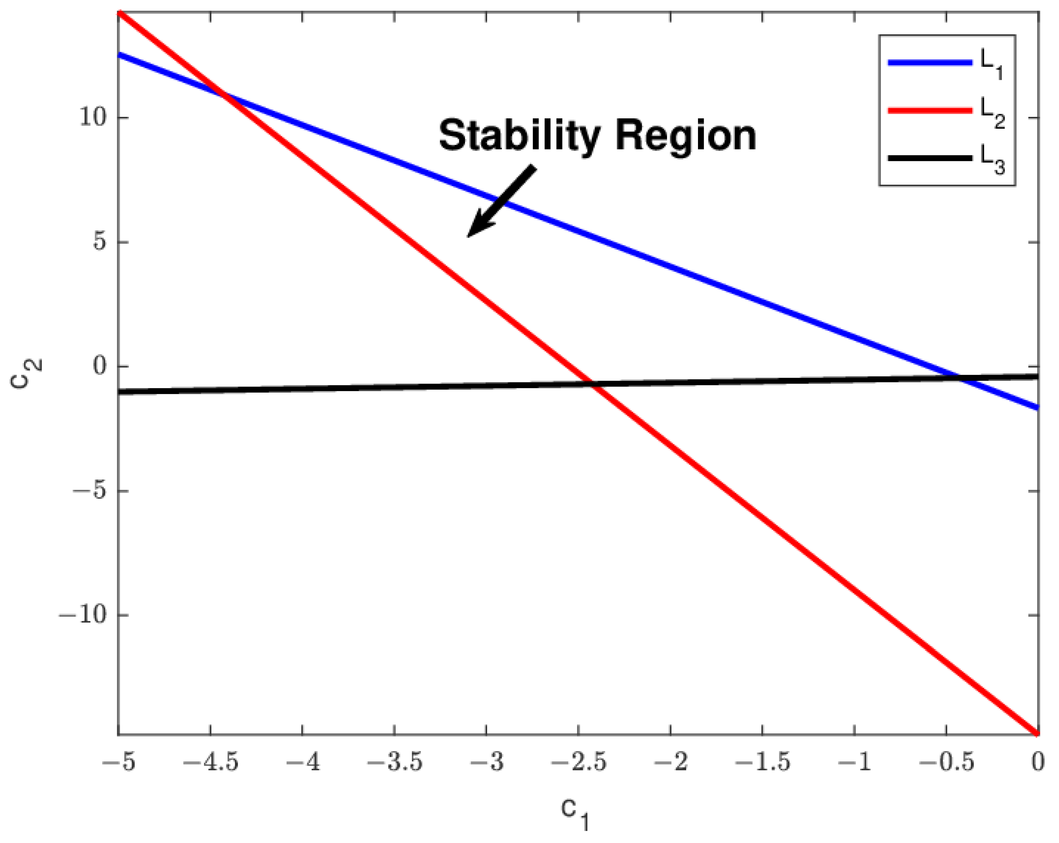
The lines of marginal stability, denoted L 1 , L 2 , and L 3 , are determined by solving λ 1 λ 2 = 1 , λ 1 = 1 , and λ 2 = 1 , respectively. These conditions ensure that the eigenvalues λ 1 and λ 2 remain inside the unit circle, i.e., | λ 1 , 2 |   < 1 . The marginal stability lines are derived as follows:
L 1 : ( 1 + A a 22 ) c 1 A a 21 c 2 = A 2 a 11 a 22 a 12 a 21 + A a 11 + a 22 , L 2 : a 22 c 1 a 21 c 2 = A a 11 a 22 a 12 a 21 , L 3 : ( A a 22 + 2 ) c 1 A a 21 c 2 = A 2 a 11 a 22 a 12 a 21 + 2 A a 11 + a 22 + 4 .
Thus, lines L 1 , L 2 , and L 3 in the ( c 1 , c 2 ) -plane define a triangular region within which | λ 1 , 2 |   < 1 .
Theorem 10.
If the feedback gains c 1 and c 2 lie within the triangular region bounded by the lines L 1 , L 2 , and L 3 , then the controller (34) is stable.

4.2. Hybrid Control Strategy

Following the hybrid control approach outlined in [31], we modify the uncontrolled model (6) into a controlled system as follows:
x n + 1 = ρ x n e h α α 1 x n ω y n k + x n σ m + x n + ( 1 ρ ) x n , y n + 1 = ρ y n e h α α γ 1 β y n k + x n + ( 1 ρ ) y n ,
where ρ ( 0 , 1 ) is a control parameter. This parameter modulates the influence of the original model (6) relative to the controlled model (36). If ρ is negative, it suggests that the controlled model may exhibit a reversed influence compared to the original model (6). On the other hand, if ρ exceeds 1, it implies that the original model has an amplified effect on the controlled model, potentially leading to impractical or undesirable behavior.
Notably, both the controlled model (36) and the uncontrolled model (6) share the same equilibrium point. The Jacobian matrix of the controlled model (36) at the interior equilibrium point ( x * , y * ) is given by
J 2 ( x * , y * ) = 1 + A ρ a 11 A ρ a 12 A ρ a 21 1 + A ρ a 22 ,
where A , a 11 , a 12 , a 21 , a 22 are defined in Equations (16) and (23). The characteristic equation of this Jacobian matrix is
λ 2 K 1 λ + K 0 = 0 ,
where the coefficients K 1 and K 0 are expressed as
K 1 = 2 + A ρ ( a 11 + a 22 ) , K 0 = ( 1 + A ρ a 11 ) ( 1 + A ρ a 22 ) A 2 ρ 2 a 12 a 21 .
The interior equilibrium ( x * , y * ) of the controlled model (36) is locally asymptotically stable if the roots of the characteristic equation lie within the open unit disk. By the Jury condition, the equilibrium point remains stable if and only if the following condition is satisfied:
| K 1 |   < 1 + K 0 < 2 .
Theorem 11.
If the condition | K 1 |   < 1 + K 0 < 2 holds, the controlled model (36) will be stable.

5. Numerical Experiments

This section provides a comprehensive analysis of specific instances of model (6), thereby validating the theoretical results presented earlier. Furthermore, numerical simulations substantiate the efficacy of both state feedback and hybrid control strategies in mitigating chaos, highlighting their practical applicability for the regulation of dynamic systems.
Example 1.
Take
α = 0.77 , ω = 0.89 , k = 2.57 , σ = 0.16 , m = 2.15 , γ = 1.32 , β = 1.42 .
With straightforward calculations, we can derive the interior equilibrium point
E 1 = ( 0.308149832276177 , 2.026866079067730 ) ,
and the bifurcation critical value
h 1 = 1.337170983163482 .
The Jacobian matrix of model (6) at the interior equilibrium point E 1 with h = h 1 is given by
J ( E 1 ) = 0.621717153436147 0.154778903236994 1.509936933944106 1.144110446200629 .
The associated eigenvalues are
λ 1 = 1 , λ 2 = 0.477606707235517 ,
noting that | λ 2 |   1 . By Theorem 8, model (6) experiences a period-doubling bifurcation at the interior equilibrium point E 1 as h passes through h 1 . This behavior, confirmed by the bifurcation diagrams shown in Figure 1, utilizes the initial conditions ( x 0 , y 0 ) = ( 0.3 , 2.1 ) and varies h over the range [ 1.2 , 2.6 ] .
Example 2.
In this example, we consider the following parameter values:
α = 0.86 , ω = 0.63 , k = 3.71 , σ = 0.89 , m = 1.78 , γ = 0.32 , β = 5.81 .
Using these parameters, we can determine the interior equilibrium point
E 1 = ( 0.501466259773058 , 0.724865104952334 ) ,
and the bifurcation critical value
h 3 = 6.005782590365195 .
The Jacobian matrix of model (6) at the interior equilibrium point E 1 with h = h 3 is given by
J ( E 1 ) = 1.188631385137408 0.407587026446246 0.299257646703919 0.738686927349767 .
The associated eigenvalues are
λ 1 , 2 = 0.963659156243587 ± 0.267134854685602 i ,
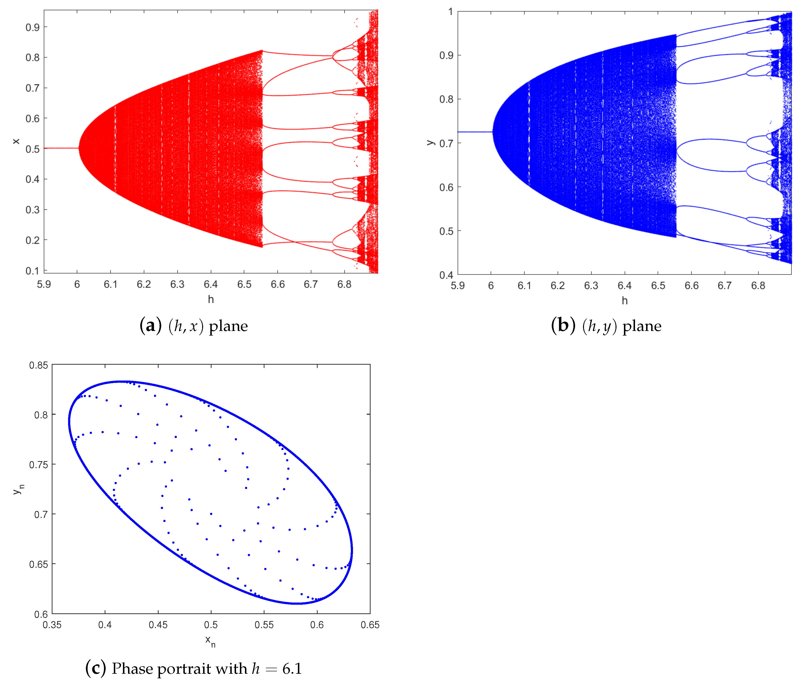
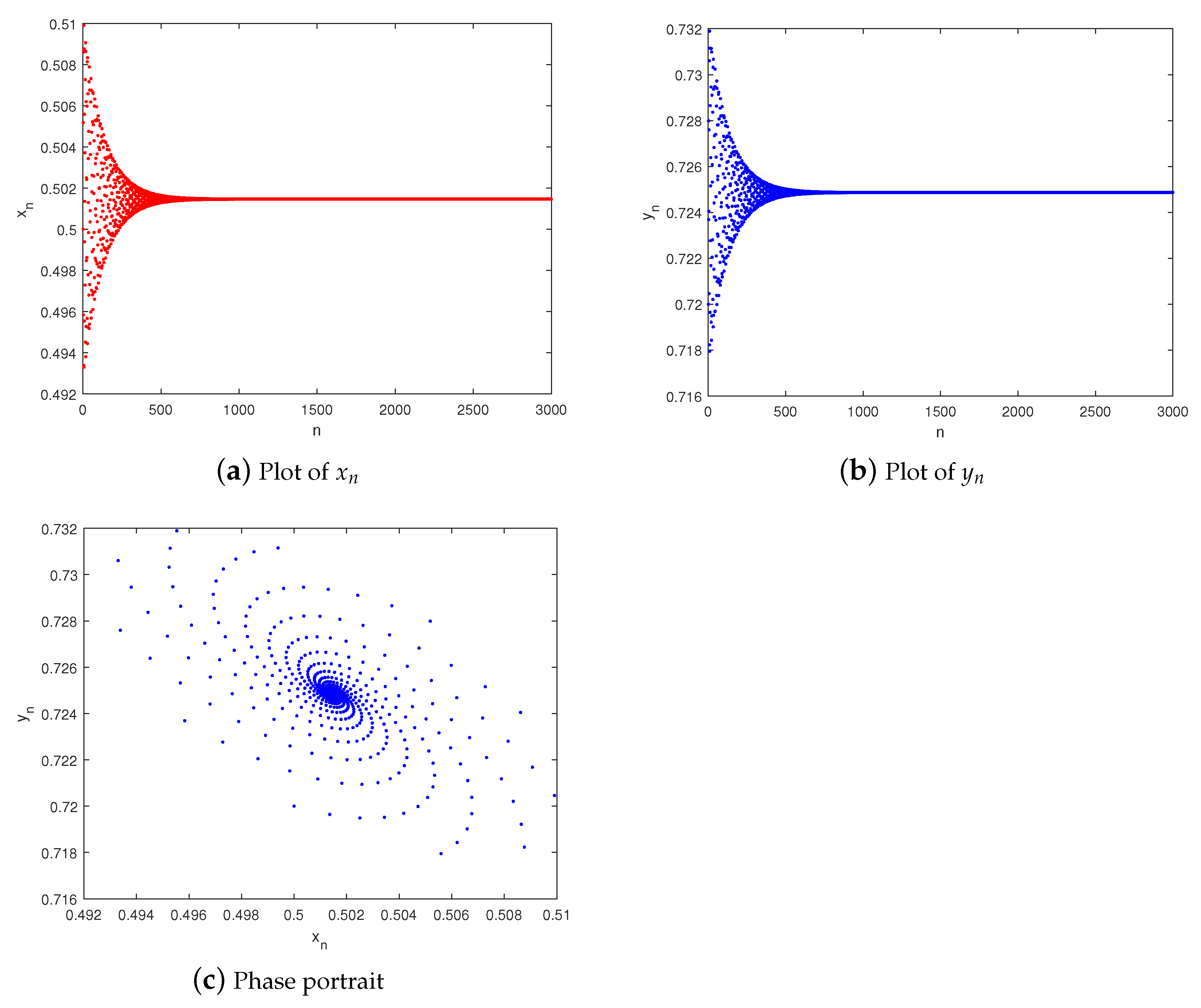
with | λ 1 , 2 |   = 1 . By Theorem 9, the model (6) experiences a Neimark–Sacker bifurcation at the interior equilibrium point E 1 as h passes through h 3 . This behavior, confirmed by the bifurcation diagrams and the phase portrait shown in Figure 2, utilizes the initial conditions ( x 0 , y 0 ) = ( 0.5 , 0.7 ) and varies h over the range [ 5.9 , 6.9 ] .
Example 3.
We begin by setting the parameters as follows:
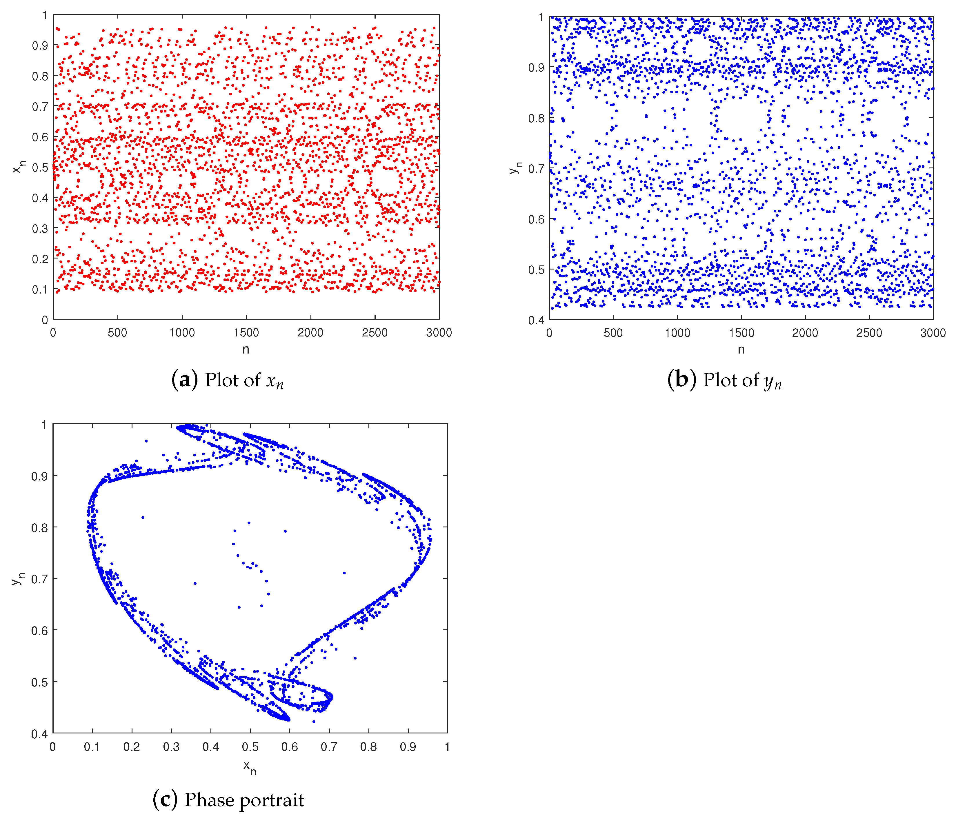
α = 0.86 , ω = 0.63 , k = 3.71 , σ = 0.89 , m = 1.78 , γ = 0.32 , β = 5.81 , h = 6.9 .
Figure 3 illustrates that, under these parameter values, the variables x n and y n in model (6) exhibit a chaotic behavior near the equilibrium point.
To address this, we apply Theorem 10 to identify a triangular region within which the feedback gains c 1 and c 2 can be chosen to control the chaotic dynamics effectively, as shown in Figure 4. Within this region, the system can be stabilized to achieve asymptotic convergence toward the equilibrium point E 1 .
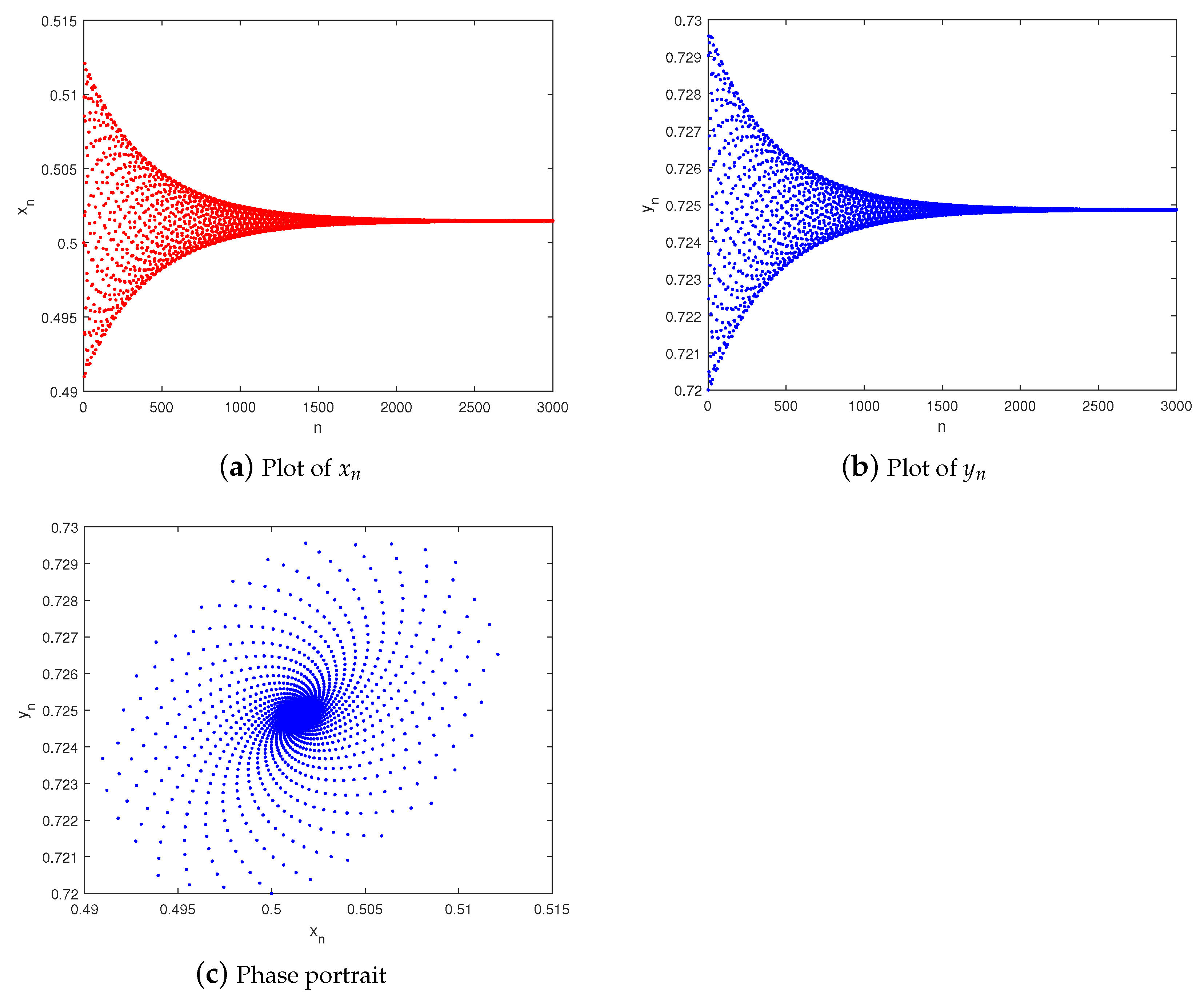
Specifically, we set c 1 = 0.98 and c 2 = 1.11 and activate the control at the 3000th iteration. As shown in Figure 5, this choice of feedback gains successfully stabilizes the chaotic trajectory, bringing it to the equilibrium point E 1 . This confirms that the feedback control approach effectively mitigates chaotic behavior, demonstrating a reliable method for managing bifurcation and suppressing chaos in the system.
Example 4.
Finally, we apply the hybrid control method to manage the chaos observed in the previous example. Using the same parameter values as in Equation (39), the Jacobian matrix of the controlled model (36), evaluated at the equilibrium point E 1 , is given by
1 2.466113036814840 ρ 0.459262206683825 ρ 0.337198483451670 ρ 1 1.959123188854205 ρ .
The characteristic polynomial corresponding to this Jacobian matrix is expressed as
λ 2 ( 2 4.425236225669045 ρ ) λ + 4.986281756360071 ρ 2 4.425236225669045 ρ + 1 = 0 .
The roots of this polynomial lie within the open unit disk if and only if 0 < ρ < 0.887482184500424 . We choose a specific value of ρ = 0.884 for the plots of x n and y n of the controlled model (36), as shown in Figure 6. From this figure, it is evident that the interior equilibrium point E 1 is stable. Thus, we conclude that the hybrid control approach is effective in mitigating bifurcation and controlling chaos within model (6).

6. Conclusions

This paper investigates the dynamical behavior of a discrete fractional modified Leslie–Gower model, incorporating a Holling-II functional response and a Michaelis–Menten-type harvesting effect. We first establish the existence and stability of nonnegative equilibrium points. Subsequently, we derive sufficient conditions for the occurrence of period-doubling and Neimark–Sacker bifurcations at the interior equilibrium point E 1 . Numerical simulations are presented, which not only validate the theoretical results but also uncover new dynamical phenomena, including the onset of chaos. To mitigate this chaotic behavior, we propose specific criteria for the implementation of state feedback and hybrid control strategies.
The findings of this study are intended to stimulate further exploration of the dynamic behavior of discrete systems, enhancing the understanding of bifurcation theory and chaos control. Moreover, these insights offer a deeper understanding of population dynamics in natural ecosystems.
In future work, we aim to extend the model to multi-species systems in order to better capture the complexities of predator–prey dynamics. Additionally, incorporating stochastic effects and environmental variability into the fractional-order model could improve its applicability to real-world ecosystems. We also plan to explore adaptive control strategies for real-time bifurcation management, which could provide valuable insights into addressing dynamic ecological challenges.

Author Contributions

Conceptualization, Y.S. and X.L.; Formal analysis, Y.S.; Funding acquisition, Y.S., X.L. and Z.W.; Investigation, Y.S. and X.L.; Validation, Y.S. and Z.W.; Writing—original draft, Y.S. and Z.W.; Writing—review and editing, Y.S. and X.L. All authors have read and agreed to the published version of the manuscript.

Funding

This research was funded by the Natural Science Foundation of Shandong Province (Grant Nos. ZR2023QF062), the National Natural Science Foundation of China (Grant Nos. 12401519), and the Central Guidance on Local Science and Technology Development Fund of Hebei Province (Grant Nos. 246Z1825G).

Data Availability Statement

Data are contained within the article.

Acknowledgments

We are grateful to the editor and reviewers for their valuable comments and suggestions, which greatly improved the presentation of this paper.

Conflicts of Interest

The authors declare no conflicts of interest.

Appendix A

a 11 = 1 + x 1 * h 1 α α 1 + ω β ( k + x 1 * ) + σ ( m + x 1 * ) 2 , a 12 = x 1 * ω h 1 α α ( k + x 1 * ) , a 13 = h 1 α α 1 + ω k β ( k + x 1 * ) 2 + m σ ( m + x 1 * ) 3 + x 1 * h 1 2 α 2 α 2 1 + ω β ( k + x 1 * ) + σ ( m + x 1 * ) 2 2 , a 14 = ω k h 1 α α ( k + x 1 * ) 2 x 1 * ω h 1 2 α α 2 ( k + x 1 * ) 1 + ω β ( k + x 1 * ) + σ ( m + x 1 * ) 2 , a 15 = x 1 * ω 2 h 1 2 α 2 α 2 ( k + x 1 * ) 2 , a 16 = h 1 α α k ω β ( k + x 1 * ) 3 m σ ( m + x 1 * ) 4 + h 1 2 α 2 α 2 1 + ω β ( k + x 1 * ) + σ ( m + x 1 * ) 2 2 x 1 * h 1 2 α α 2 ω β ( k + x 1 * ) 2 + σ ( m + x 1 * ) 3 1 + ω β ( k + x 1 * ) + σ ( m + x 1 * ) 2 + x 1 * h 1 3 α 6 α 3 1 + ω β ( k + x 1 * ) + σ ( m + x 1 * ) 2 3 , a 17 = ω k h 1 α α ( k + x 1 * ) 3 + h 1 2 α α 2 ( k + x 1 * ) 2 k ω ω 2 ( k x 1 * ) β ( k + x 1 * ) σ ω ( k m x 1 * 2 ) ( m + x 1 * ) 3 + x 1 * ω h 1 3 α 2 α 3 ( k + x 1 * ) 1 + ω β ( k + x 1 * ) + σ ( m + x 1 * ) 2 2 , a 18 = ω 2 ( k x 1 * ) h 1 2 α 2 α 2 ( k + x 1 * ) 3 + x 1 * ω 2 h 1 3 α 2 α 3 ( k + x 1 * ) 2 1 + ω β ( k + x 1 * ) + σ ( m + x 1 * ) 2 , a 19 = x 1 * ω 3 h 1 3 α 6 α 3 ( k + x 1 * ) 3 , b 11 = h 1 α 1 1 2 x 1 * k ω β ( k + x 1 * ) m σ ( m + x 1 * ) 2 , b 12 = ω x 1 * h 1 α 1 k + x 1 * , b 13 = 0 , b 15 = x 1 * ω 2 h 1 2 α 1 α ( k + x 1 * ) 2 , b 16 = ω k h 1 α 1 ( k + x 1 * ) 2 , b 17 = 0 , b 14 = h 1 α 1 1 + ω k β ( k + x 1 * ) 2 + m σ ( m + x 1 * ) 3 + x 1 * h 1 2 α 1 α 1 + ω β ( k + x 1 * ) + σ ( m + x 1 * ) 2 2 , b 18 = x 1 * ( α 1 ) h 1 α 2 2 1 + ω β ( k + x 1 * ) + σ ( m + x 1 * ) 2 , b 19 = x 1 * ( α 1 ) ω h 1 α 2 2 ( k + x 1 * ) , a 21 = γ h 1 α β α , a 22 = 1 γ h 1 α α , a 23 = γ h 1 α ( k + x 1 * ) β α + γ 2 h 2 α 2 β α 2 ( k + x 1 * ) , a 24 = 2 γ h α α ( k + x 1 * ) β 2 h 2 α α 2 ( k + x 1 * ) , a 25 = γ β h α α ( k + x 1 * ) + γ β 2 h 2 α 2 α 2 ( k + x 1 * ) , a 26 = γ h α β α ( k + x 1 * ) 2 γ 2 h 2 α β α 2 ( k + x 1 * ) 2 + γ 3 h 3 α 6 β α 3 ( k + x 1 * ) 2 , a 27 = 2 h α γ α ( k + x 1 * ) 2 + 5 γ 2 h 2 α 2 α 2 ( k + x 1 * ) 2 γ 3 h 3 α 2 α 3 ( k + x 1 * ) 2 , a 28 = h α γ β α ( k + x 1 * ) 2 2 γ 2 β h 2 α α 2 ( k + x 1 * ) 2 + γ 3 β h 3 α 2 α 3 ( k + x 1 * ) 2 , a 29 = γ 2 β 2 h 2 α 2 α 2 ( k + x 1 * ) 2 γ 3 β 2 h 3 α 6 α 3 ( k + x 1 * ) 2 , b 21 = γ h α 1 β , b 22 = γ h α 1 , b 23 = 0 , b 24 = γ h α 1 ( k + x 1 * ) β + γ 2 h 2 α 1 β α ( k + x 1 * ) , b 25 = γ β h α 1 k + x 1 * + γ 2 β h 2 α 1 α ( k + x 1 * ) , b 26 = 2 γ h α 1 ( k + x 1 * ) 2 γ 2 h 2 α 1 α ( k + x 1 * ) , b 27 = 0 , b 28 = ( α 1 ) γ h α 2 2 β , b 29 = ( α 1 ) γ h α 2 2 .

References

  1. Lotka, A.J. Contribution to the theory of periodic reaction. J. Phys. Chem. 1910, 14, 271–274. [Google Scholar] [CrossRef]
  2. Volterra, V. Variazioni e fluttuazioni del numero d’individui in specie animali conviventi. Mem. R. Accad. Naz. Lincei. 1926, 2, 31–113. [Google Scholar]
  3. Volterra, V. Variations and fluctuations of the number of individuals in animal species living together. Anim. Ecol. 1931, 412–433. [Google Scholar] [CrossRef]
  4. Holling, C.S. The components of predation as revealed by a study of small-mammal predation of the European pine sawfly. Can. Entomol. 1959, 91, 293–320. [Google Scholar] [CrossRef]
  5. Holling, C.S. Some characteristics of simple types of predation and parasitism. Can. Entomol. 1959, 91, 385–398. [Google Scholar] [CrossRef]
  6. Leslie, P.H. Some further notes on the use of matrices in population mathematics. Biometrika 1948, 35, 213–245. [Google Scholar] [CrossRef]
  7. Leslie, P.H.; Gower, J.C. The properties of a stochastic model for the predator-prey type of interaction between two species. Biometrika 1960, 47, 219–234. [Google Scholar] [CrossRef]
  8. May, R. Stability and complexity in model ecosystems. In Monographs in Population Biology; Princeton University Press: Princeton, NJ, USA, 1974. [Google Scholar]
  9. Gupta, R.P.; Chandra, P. Bifurcation analysis of modified Leslie-Gower predator-prey model with Michaelis-Menten type prey harvesting. J. Math. Anal. Appl. 2013, 398, 278–295. [Google Scholar] [CrossRef]
  10. Hu, D.; Cao, H. Stability and bifurcation analysis in a predator-prey system with Michaelis-Menten type predator harvesting. Nonlinear Anal. Real World Appl. 2017, 33, 58–82. [Google Scholar] [CrossRef]
  11. Song, Q.; Yang, R.; Zhang, C.; Tang, L. Bifurcation analysis in a diffusive predator-prey system with Michaelis-Menten-type predator harvesting. Adv. Differ. Equ. 2018, 329, 2018. [Google Scholar] [CrossRef]
  12. Singh, A.; Malik, P. Bifurcations in a modified Leslie-Gower predator-prey discrete model with Michaelis-Menten prey harvesting. J. Appl. Math. Comput. 2021, 67, 143–174. [Google Scholar] [CrossRef]
  13. Chen, J.; Zhu, Z.; He, X.; Chen, F. Bifurcation and chaos in a discrete predator-prey system of Leslie type with Michaelis-Menten prey harvesting. Open Math. 2022, 20, 608–628. [Google Scholar] [CrossRef]
  14. Khan, M.S.; Abbas, M.; Bonyah, E.; Qi, H. Michaelis-Menten-type prey harvesting in discrete modified Leslie-Gower predator-prey model. J. Funct. Spaces 2022, 2022, 9575638. [Google Scholar] [CrossRef]
  15. Han, X.; Du, X. Dynamics study of nonlinear discrete predator-prey system with Michaelis-Menten type harvesting. Math. Biosci. Eng. 2023, 20, 16939–16961. [Google Scholar] [CrossRef]
  16. Shi, Y.; Ma, Q.; Ding, X. Dynamical behaviors in a discrete fractional-order predator-prey system. Filomat 2018, 32, 5857–5874. [Google Scholar] [CrossRef]
  17. Moustafa, M.; Mohd, M.H.; Ismail, A.I.; Abdullah, F.A. Dynamical analysis of a fractional-order eco-epidemiological model with disease in prey population. Adv. Differ. Equ. 2020, 2020, 1–24. [Google Scholar] [CrossRef]
  18. Arif, M.S.; Abodayeh, K.; Ejaz, A. Stability analysis of fractional-order predator-prey system with consuming food resource. Axioms 2023, 12, 64. [Google Scholar] [CrossRef]
  19. Wang, B.; Li, X. Modeling and dynamical analysis of a fractional-order predator-prey system with anti-predator behavior and a Holling type IV functional response. Fractals Fract. 2023, 7, 722. [Google Scholar] [CrossRef]
  20. Xu, C.; Cui, X.; Li, P.; Yan, J.; Yao, L. Exploration on dynamics in a discrete predatorprey competitive model involving feedback controls. J. Biol. Dyn. 2023, 17, 2220349. [Google Scholar] [CrossRef]
  21. Xu, C.; Mu, D.; Pan, Y.; Aouiti, C.; Yao, L. Exploring bifurcation in a fractional-order predator-prey system with mixed delays. J. Appl. Anal. Comput. 2023, 13, 1119–1136. [Google Scholar] [CrossRef]
  22. Xu, C.; Cui, Q.; Liu, Z.; Pan, Y.; Cui, X.; Ou, W.; Rahman, M.U.; Farman, M.; Ahmad, S.; Zeb, A. Extended hybrid controller design of bifurcation in a delayed chemostat model. MATCH Commun. Math. Comput. Chem. 2023, 90, 609–648. [Google Scholar] [CrossRef]
  23. Zhang, Y.; Li, P.; Xu, C.; Peng, X.; Qiao, R. Investigating the effects of a fractional operator on the evolution of the enso model: Bifurcations, stability and numerical analysis. Fractal Fract. 2023, 7, 602. [Google Scholar] [CrossRef]
  24. Li, B.; Eskandari, Z.; Avazzadeh, Z. Dynamical behaviors of an SIR epidemic model with discrete time. Fractal Fract. 2022, 6, 659. [Google Scholar] [CrossRef]
  25. Tassaddiq, A.; Shabbir, M.S.; Din, Q.; Naaz, H. Discretization, bifurcation, and control for a class of predator-prey interactions. Fractal Fract. 2020, 6, 31. [Google Scholar] [CrossRef]
  26. Rahmi, E.; Darti, I.; Suryanto, A.; Trisilowati. A modified Leslie-Gower model incorporating Beddington-DeAngelis functional response, double Allee effect and memory effect. Fractal Fract. 2021, 5, 84. [Google Scholar] [CrossRef]
  27. Khalil, R.; Al Horani, M.; Yousef, A.; Sababheh, M. A new definition of fractional derivative. J. Comput. Appl. Math. 2014, 264, 65–70. [Google Scholar] [CrossRef]
  28. Abdeljawad, T. On conformable fractional calculus. J. Comput. Appl. Math. 2015, 279, 57–66. [Google Scholar] [CrossRef]
  29. Kuzenetsov, Y.A. Elements of Applied Bifurcation Theory, 4th ed.; Springer: New York, NY, USA, 2023; pp. 129–173. [Google Scholar]
  30. Shi, Y.; Wang, Z. Bifurcation analysis and chaos control of a discrete fractional-order Leslie-Gower model with fear factor. AIMS Math. 2024, 9, 30298–30319. [Google Scholar] [CrossRef]
  31. Singh, A.; Sharma, V.S. Bifurcations and chaos control in a discrete-time prey-predator model with Holling type-II functional response and prey refuge. J. Comput. Appl. Math. 2023, 418, 114666. [Google Scholar] [CrossRef]
  32. Berkal, M.; Almatrafi, M.B. Bifurcation and stability of two-dimensional activator-inhibitor model with fractional-order derivative. Fractal Fract. 2023, 7, 344. [Google Scholar] [CrossRef]
  33. Saadeh, R.; Abbes, A.; Al-Husban, A.; Ouannas, A.; Grassi, G. The fractional discrete predator-prey model: Chaos, control and synchronization. Fractal Fract. 2023, 7, 120. [Google Scholar] [CrossRef]
  34. Din, Q.; Naseem, R.A.; Shabbir, M.S. Predator-prey interaction with fear effects: Stability, bifurcation and two-parameter analysis incorporating complex and fractal behavior. Fractal Fract. 2024, 8, 221. [Google Scholar] [CrossRef]
  35. Ishaque, W.; Din, Q.; Khan, K.; Mabela, R. Dynamics of predator-prey model based on fear effect with bifurcation analysis and chaos control. Qual. Theory Dyn. Syst. 2024, 23, 26. [Google Scholar] [CrossRef]
  36. Wiener, J. Differential Equations with Piecewise Constant Delays, Trends in Theory and Practice of Nonlinear Differential Equations: Lecture Notes in Pure and Applied Math; Dekke: New York, NY, USA, 1984. [Google Scholar]
  37. Luo, A.C.J. Regularity and Complexity in Dynamical Systems; Springer: New York, NY, USA, 2012. [Google Scholar]
  38. Guckenheimer, J.; Holmes, P. Nonlinear Oscillations, Dynamical Systems, and Bifurcations of Vector Fields; Springer: New York, NY, USA, 1983. [Google Scholar]
  39. Luo, X.S.; Chen, G.; Wang, B.H.; Fang, J.Q. Hybrid control of period-doubling bifurcation and chaos in discrete nonlinear dynamical systems. Chaos Solitons Fractals 2003, 18, 775–783. [Google Scholar] [CrossRef]
  40. Din, Q. Compexity and chaos control in a discrete-time prey-predator model. Commun. Nonlinear Sci. Numer. Simul. 2017, 49, 113–134. [Google Scholar] [CrossRef]
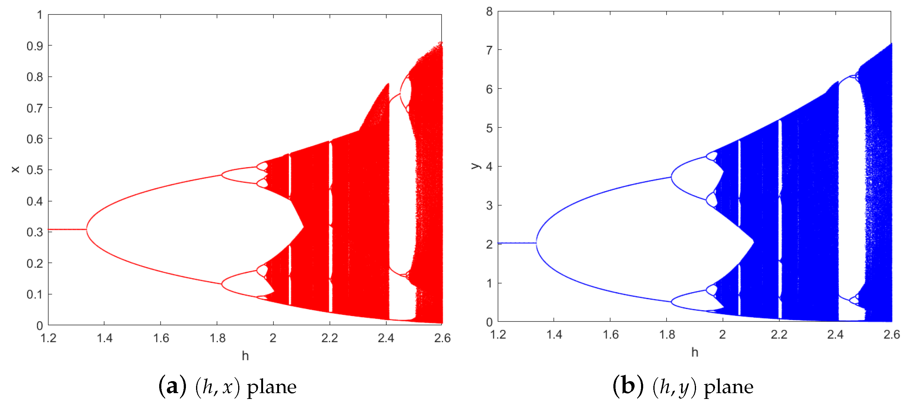
Figure 1. Period-doubling bifurcation diagrams for model (6), with the parameter values given by Equation (38) and the initial conditions ( 0.3 , 2.1 ) .
Fractalfract 08 00744 g001
Figure 2. Neimark–Sacker bifurcation diagrams and phase portrait for model (6), with the parameter values given by Equation (39) and the initial conditions ( 0.5 , 0.7 ) .
Fractalfract 08 00744 g002
Figure 3. Plots for model (6) with the parameter values given by Equation (40) and the initial conditions ( 0.50 , 0.72 ) .
Fractalfract 08 00744 g003
Figure 4. Stability region for the controlled model (34).
Fractalfract 08 00744 g004
Figure 5. Plots for the controlled model (34) with the parameter values given by Equation (40), c 1 = 0.98 , c 2 = 1.11 , and the initial conditions ( 0.50 , 0.72 ) .
Fractalfract 08 00744 g005
Figure 6. Plots for the controlled model (36) with the parameter values given by Equation (40), ρ = 0.884 , and the initial conditions ( 0.50 , 0.72 ) .
Fractalfract 08 00744 g006
Table 1. Biological interpretation of all parameters in model (1).
ParametersInterpretation
X , Y the prey and predator species densities, respectively
rthe prey species’ intrinsic growth rate
Kthe environment’s maximum carrying capacity for the prey species
a 1 the rate at which the prey is consumed
nthe half-saturation constant
qthe prey catchability coefficient
Ethe harvesting effort applied to capture individuals
m 1 , 2 suitable positive constants
sthe predator species’ intrinsic growth rate
s a 2 the maximum per capita reduction rate of the predator
Disclaimer/Publisher’s Note: The statements, opinions and data contained in all publications are solely those of the individual author(s) and contributor(s) and not of MDPI and/or the editor(s). MDPI and/or the editor(s) disclaim responsibility for any injury to people or property resulting from any ideas, methods, instructions or products referred to in the content.