Analysis and Warning Prediction of Tunnel Deformation Based on Multifractal Theory

Abstract

To better analyze the fluctuation characteristics and development law of tunnel deformation data, multifractal theory is applied to tunnel deformation analysis. That is, the multifractal detrended fluctuation analysis (MF-DFA) model is first utilized to carry out the multifractal characterization of tunnel deformation data. Further, Mann–Kendall (M–K) analysis is utilized to construct the dual criterion (∆α indicator criterion and ∆f(α) indicator criterion) for the tunnel deformation early warning study. In addition, the particle swarm optimization long-short-term memory (PSO-LSTM) prediction model is used for predicting tunnel settlement. The results show that, in reference to the tunnel warning level criteria and based on the Z-value results of the indicator criterion, the warning level of all four sections is class II. At the same time, through the analysis of tunnel settlement predictions, the PSO-LSTM model has a better prediction effect and stability for tunnel settlement. The predicted results show a slow increase in tunnel settlement over the next 5 days. Finally, the tunnel warning level and the predicted results of tunnel settlement are analyzed in a comprehensive manner. The deformation will increase slowly in the future. Therefore, monitoring and measurement should be strengthened, and disaster preparedness plans should be prepared.

1. Introduction

With the continuous development of transportation construction in China, the scale and technical level of tunnel construction have reached new heights [1]. By the end of 2022, the national railroad operating mileage reached 155,000 km, boasting 17,873 operational railroad tunnels with a cumulative length of approximately 22,000 km. Of these, 259 extra-long railroad tunnels and 12 tunnels exceeding 20 km in length are in operation [2]. Notably, over the past five years, railroad tunnel development has experienced remarkable acceleration. This surge is attributed to the rapid growth of the high-speed railroad industry and the consistent enhancement of tunnel trimming technology, resulting in the emergence of numerous tunnels traversing diverse types of special strata [3]. However, concurrent with this progress, there exist design and construction irregularities in high-speed railroad tunnels that may lead to deformation, water leakage, cracking, and other issues [4,5,6,7,8].

In tunnel construction, the control of tunnel deformation stands out as pivotal technology [9]. Consequently, the monitoring and stability evaluation of tunnel deformation are paramount. Current methods for deformation monitoring and analysis encompass numerical simulation methods [10,11,12,13], time series analysis methods [14,15,16,17], fuzzy comprehensive evaluation methods [18,19,20,21], and machine learning methods [22,23,24,25]. Yet, the complexity of the geological environment and deformation-inducing factors introduce a nonlinear characteristic to the tunnel deformation monitoring time-course curve, causing fluctuations [26]. Therefore, the multifractal detrended fluctuation analysis (MF-DFA) method presents an effective approach for tunnel deformation analysis.

Fractal theory, pioneered by the French mathematicians Mandelbrot et al. [27], describes chaotic, complex, and self-similar systems with regularity. Researchers, such as Zuo et al., have applied fractal theory to analyze and predict tunnel surface settlement, evaluating surface settlement stability [28]. Ye et al. established a model based on fractal theory to study the interaction between microstructure evolution and tunnel leakage behavior, offering insight into the tunnel leakage mechanism [29]. Additionally, MF-DFA, initially proposed by Grassberger [30], finely describes the volatility of tunnel deformation monitoring data at different levels. At present, the multifractal theory has been widely used. Lei et al. used multifractal theory and subcomponent combination prediction to synthesize the warning level of landslides [31]. Mao et al. revealed early warning signals of rock slope deformation based on the multiple fractal time-varying response characteristics of micro-seismic waveforms associated with rock rupture [32]. Zhou et al. applied multifractal theory to the deformation pattern analysis of dams and utilized MF-DFA, multivariate multifractal detrended fluctuation analysis (MV-MFDFA), and asymmetric multifractal detrended fluctuation analysis (A-MFDFA) to resolve the multiple fractal features of deformation states and their asymmetry [33].

Accurate prediction of tunnel deformation is crucial for disaster prevention and early warning. Currently, soil settlement prediction methods include empirical methods [34,35,36], theoretical methods [37,38,39,40], modeling methods [41,42,43,44], and machine learning methods [45,46,47,48]. Long short-term memory (LSTM) is particularly effective in handing time-related information and is widely used in temporal tunnel settlement prediction [49]. Li et al. employed three machine learning algorithms (LSTM, RF, and GRU) to forecast surface settlement. Their findings indicated that the LSTM algorithm demonstrated superior accuracy in predicting maximum surface settlement and effectively anticipated settlement progression in various strata [50]. Cao et al. proposed the complete ensemble empirical mode decomposition with adaptive noise long short-term memory (CEEMDAN-LSTM) model, combining high prediction accuracy with acceptable computational efficiency [51]. Duan et al. utilized the auto regressive integrated moving average (ARIMA) and LSTM models for predicting structural deformation trends during tunnel operation, determining that LSTM performs better with high data quality and sufficient samples [52].

From the above research results, it can be concluded that research on tunnel deformation analysis and early warning prediction is necessary. Therefore, this paper analyzes tunnel deformation data. Firstly, the deformation rate and the deformation of the tunnel are investigated by multiple fractal characterizations using MF-DFA. Secondly, the Mann–Kendall (M–K) analysis method [53,54] is used to evaluate the early warning classification of tunnel deformation. Furthermore, the prediction of tunnel deformation is realized by the particle swarm optimization LSTM (PSO-LSTM) prediction model. Finally, the results of tunnel deformation early warning classification and the tunnel deformation prediction results are jointly addressed. The tunnel deformation law is evaluated comprehensively to provide theoretical guidance for its monitoring, measurement, and prevention. This study calculates and analyzes the multifractal features of tunnel monitoring data by integrating the M–K method to determine the tunnel’s warning level. Furthermore, the PSO-LSTM model is found to exhibit high accuracy in predicting tunnel deformation, offering a novel perspective for advancing research on tunnel early warning prediction.

2. Materials and Methods

The process of tunnel deformation analysis and early warning prediction, established in this paper based on multiple fractal theory, is illustrated in Figure 1. The steps can be summarized as follows:

First, tunnel deformation monitoring and measurement are conducted to obtain tunnel deformation data. Second, the monitoring data are segmented into 12 groups, and multifractal eigenvalues are calculated and analyzed using the M–K method. The warning level is then determined in conjunction with the warning level criteria. Third, the parameters of the LSTM prediction model are optimized using the PSO optimization algorithm, and the PSO-LSTM prediction model is formulated for predicting tunnel settlement. Fourth, the warning level and prediction results are jointly analyzed to obtain the warning outcomes. Finally, corresponding preventive measures are implemented based on the results of the warning level.

This comprehensive approach provides a systematic framework for tunnel deformation analysis, early warning prediction, and subsequent preventive action.

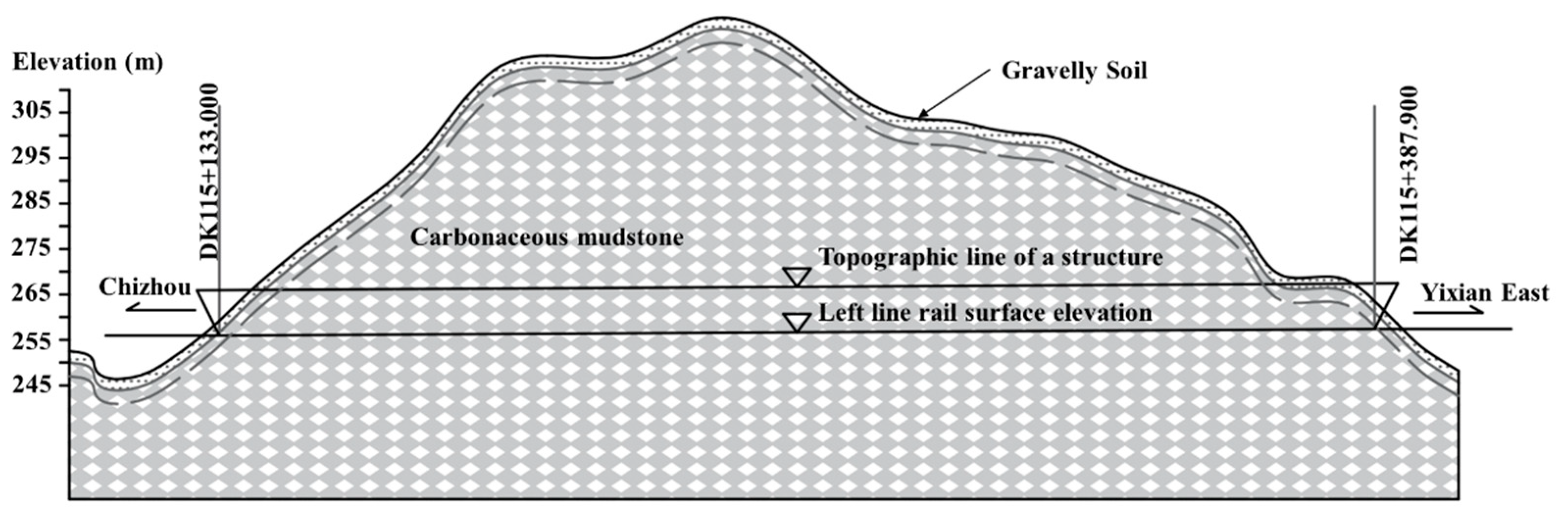
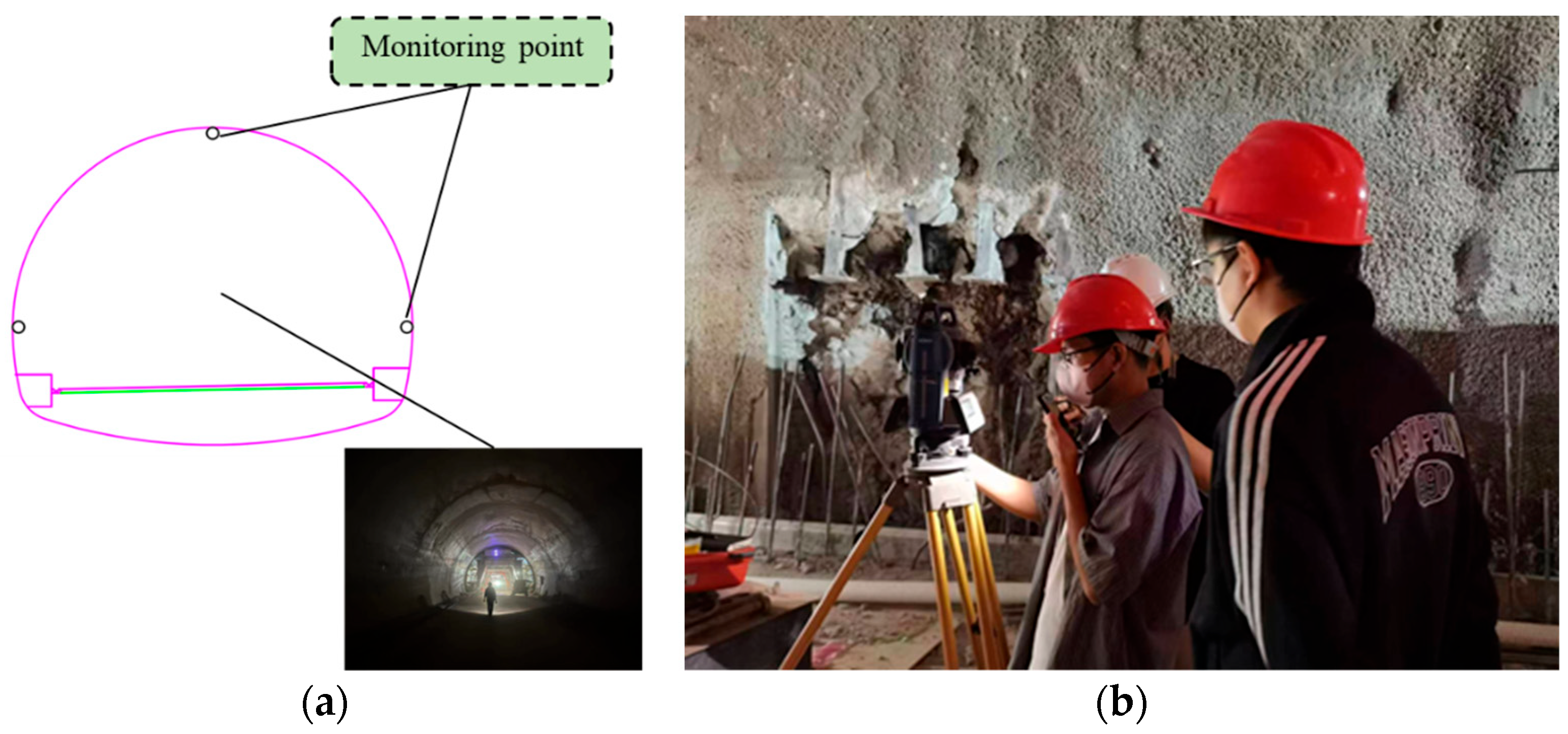
2.1. Project Overview and Monitoring Data

The high-speed rail tunnel has a total length of 254.9 m, with the starting and ending mileage marked as DK115 + 133.0~DK115 + 387.9. It is positioned between the Sangujian No. 1 Tunnel and the Xikeng bridge. Geographically, it is situated on the western side of the mountain, in Tamkou Village, Xidi Town, Yixian County, Huangshan City. The surface vegetation on the mountain is characterized by bamboo forests, low shrubs, trees, and low weeds. The terrain is steep, with a natural slope ranging from 30° to approximately 55°. The tunnel is surrounded by dense mountain vegetation, and the entrance and exit are marked by ravine confluence, making traffic inconvenient. The perimeter rock grade is classified as IV, and the excavation employs the three-step method.

The tunnel is situated in the low hills, originating from Huangshan Mountain. It is characterized by undulating terrain with mountain elevations ranging from 250 m to 325 m and a maximum elevation difference of approximately 75 m. The mountain exhibits a monoclinic structure, with steeper south and north slopes. The tunnel primarily traverses carbonaceous mudstone of the Cambrian Hotang formation, with a maximum tunnel depth of about 65 m. (Refer to Figure 2 for a visualization of the tunnel cross-section.)

To ensure the safety of tunnel construction operations, a total station is utilized for manual measurement of tunnel settlement and convergence. This paper involves monitoring the settlement of the tunnel vault and tunnel convergence utilizing the rear rendezvous method and the opposite side measurement method, respectively. For arch settlement monitoring, a single monitoring point is positioned at the arch of each section. In contrast, for tunnel convergence monitoring, two monitoring points are symmetrically arranged on both sides of the tunnel, employing the opposite side measurement method. Consequently, three monitoring points are allocated in each section, with a monitoring frequency of 2 times/day. Further details are depicted in Figure 3.

As shown in Figure 4 and Figure 5, this paper examines the monitoring data regarding tunnel settlement and convergence in the section from DK115 + 261~DK115 + 290. Additionally, the data from monitoring points are counted. The cumulative deformation–time diagram and deformation rate–time diagram of tunnel settlement and convergence are obtained, respectively.

In Figure 4, it is evident that both the cumulative tunnel settlement deformation and the cumulative tunnel convergence deformation exhibit an increasing trend over time. Notably, after 1000 h, the growth of these deformation measures reaches a turning point, transitioning into a slower growth trend. Throughout the monitoring period, the data display both significant and minor fluctuations, which can be effectively analyzed using multiple fractal theory.

Looking at Figure 5, it is apparent that both the tunnel settlement deformation rate and the tunnel convergence deformation rate demonstrate significant and minor fluctuations, displaying the characteristic traits of multiple fractals. These fluctuations can be effectively analyzed using multiple fractal theory.

2.2. MF-DFA

The MF-DFA model, which belongs to the multiple non-uniform fractal method, not only reveals the multiple fractal characteristics within the deformation sequence but also effectively evaluates their deformation trends [55]. The calculation steps are as follows:

Step 1: the data presented in Figure 4 and Figure 5, respectively, are set as a time series $x\left(t\right)$ with a series length of N, a series mean of $\overline{x}$, and a series of cumulative deviations of $x\left(t\right)$ with respect to $\overline{x}$ as $y\left(t\right)$:

$$y\left(t\right)=\sum _{i=1}^t(x\left(i\right)-\overline{x})$$

(1)

Step 2: Set a time scale $s$. Equalize the sequence $y\left(t\right)$ in terms of $s$, dividing it into a total of $m$ equal-length consecutive and non-overlapping sub-intervals, $m=int(N/s)$.

In practical arithmetic, $N$ may not necessarily be divisible, resulting in potential tail data redundancy. Thus, alongside positive-order division, a reverse-order processing method is also employed simultaneously. The division operation is repeated from the end of the sequence to obtain $2m$ subintervals.

Step 3: Fit a trend to each subinterval and subtract the trend portion from the original. Obtain the corresponding residual series denoted as $z_v\left(t\right)$:

$$z_v\left(t\right)=y_v\left(t\right)-p_v^k\left(t\right)$$

(2)

where $y_v\left(t\right)$ represents the subinterval, and $p_v^k\left(t\right)$ is a kth order fitting polynomial to the vth subinterval. $v$ ranges from 1 to 2 m, and $t$ ranges from 1 to s.

Step 4: calculate the mean square deviation $F^2(s,v)$ of the residual sequence $z_v\left(t\right)$:

$$F^2\left(s,v\right)=\frac{1}{s}\sum _{t=1}^s{\left(z_v\right(t\left)\right)}^2$$

(3)

Step 5: Optimize the traditional MF-DFA division by employing a sliding window, which involves moving the values through a window of a specific length along the sequence at a defined step size. This helps to minimize pseudo-fluctuations in the data and maximize the utilization of data information.

The window length is denoted as s, the sequence length as N, and the sliding step is set to 1. The number of subintervals obtained in one run is N − S + 1, and the q-order fluctuation function is calculated according to Equation (4):

$$F_q\left(s\right)=\left\{\begin{array}{c}{\left\{\frac{1}{N-s+1}{\displaystyle \sum _{v=1}^{N-s+1}}{\left[F^2\right(s,v\left)\right]}^{q/2}\right\}}^{1/q},q\ne 0\\ \exp \left\{\frac{1}{2\left(N-s+1\right)}{\displaystyle \sum _{v=1}^{N-s+1}}\ln \left[F^2\left(s,v\right)\right]\right\},q=0\end{array}\right.$$

(4)

Step 6: Repeat the previous steps to generate a series of point values for $s$-$F_q\left(s\right)$. If this time series exhibits a long-range correction, then $F_q\left(s\right)$ has a power-law relationship with $s,$ as shown in Equation (5):

$$F_q\left(s\right)\propto s^{h\left(q\right)}$$

(5)

By taking the logarithms of both sides of the previous equation, we obtain Equation (6):

$$lg{F}_q\left(s\right)=h\left(q\right)lgs+lgb$$

(6)

where $F_q\left(s\right)$ represents the $q$-order fluctuation function of the series, $h\left(q\right)$ is the corresponding generalized Hurst exponent, and $b$ is a constant coefficient.

A plot of $lg{F}_q\left(s\right)$-$lgs$ was created and fitted to determine the generalized Hurst exponent $h\left(q\right)$. A fixed $h\left(q\right)$ suggests a mono-fractal sequence without multifractal features. When $h\left(q\right)<0.5$, the data sequence behaves as a memory process with inverse persistence. A value of $h\left(q\right)=0.5$ indicates uncorrelated stochastic behavior. For $h\left(q\right)>0.5$, the data sequence behaves as a memory process with positive persistence. Values of $h\left(q\right)>1$ indicate long-range positively correlated processes with strong non-stationarity.

Step 7: the multifractal spectrum $f\left(\alpha \right)$, which characterizes the fractal intensity and singularity of the time series, can typically be determined using Equation (7):

$$\left\{\begin{array}{c}\tau \left(q\right)=qh\left(q\right)-1\\ \alpha ={\tau }^{\prime }\left(q\right)\\ f\left(\alpha \right)=q\alpha -\tau \left(q\right)\end{array}\right.$$

(7)

where $\tau \left(q\right)$ is the Renyi index, also known as the scalar function. If it is a nonlinear up-convex function of $q$, the displacement sequence exhibits multifractal characteristics. If it is a linear function of $q$, the displacement sequence exhibits single fractal characteristics.

Step 8: calculate the multifractal spectral parameter $∆\alpha$ and $∆f\left(\alpha \right)$.

$$\left\{\begin{array}{c}∆\alpha ={\alpha }_{max}-{\alpha }_{min}\\ ∆f\left(\alpha \right)=∆f\left({\alpha }_{max}\right)-∆f\left({\alpha }_{min}\right)\end{array}\right.$$

(8)

where the $∆\alpha$ parameter is mainly used to evaluate the width of the multifractal spectrum of the data deformation sequence. As the value of $∆\alpha$ increases, the intensity of multiple fractals becomes stronger, leading to more intense fluctuations. The $∆f\left(\alpha \right)$ parameter is mainly used to evaluate the proportion of large and small fluctuations in the waveform of the data deformation sequence. As the value of $∆f\left(\alpha \right)$ decreases, the proportion of large fluctuation waveforms increases.

2.3. M–K Test Method

The M–K test method is a non-parametric method. Non-parametric tests are also known as non-distributional tests. It has the advantage that the sample does not have to follow a particular distribution and is not affected by a few outliers. It is suitable for type and order variables, and it is relatively simple to calculate [56]. The specific calculation steps are as follows:

Step 1: The 12 sets of eigenvalues obtained from each set of data by the formula in 2.2 are set as a time series of 12 sample sizes $\left\{x_1,x_2,\dots \dots ,x_{12}\right\}$. For all $k$($j\le n$ and $k\ne j$), the distributions of $x_k$ and $x_j$ are different and the difference function $Sgn\left(x_j-x_k\right)$ is computed:

$$Sgn\left(x_j-x_k\right)=\left\{\begin{array}{cc}+1,& \left(x_j-x_k\right)>0\\ 0,& \left(x_j-x_k\right)=0\\ -1,& \left(x_j-x_k\right)<0\end{array}\right.$$

(9)

Step 2: calculate the test statistic $S$:

$$S=\sum _{k=1}^{n-1}\sum _{j=k+1}^{n}Sgn(x_j-x_k)$$

(10)

Step 3: $S$ is normally distributed with mean 0. Calculate the variance $Var\left(S\right)$:

$$Var\left(s\right)=\frac{n(n-1)(2n+5)}{18}$$

(11)

Step 4: calculate the standard normal statistical variable $Z$:

$$Z=\left\{\begin{array}{cc}\frac{S-1}{\sqrt{Var\left(s\right)}},& S>0\\ 0,& S=0\\ \frac{S+1}{\sqrt{Var\left(s\right)}},& S<0\end{array}\right.$$

(12)

Step 5: The trend characteristics of the corresponding evaluation object can be judged by the size of Z. The $Z_{\alpha }$ value is the critical value under the condition of corresponding significant level α. In this paper, the significance test with 99% confidence level is selected. That is, for a significance level $\alpha =0.01$, then $Z_{0.01}=2.32$.

If $Z\ge Z_{\alpha }$, it means that the evaluation object has an increasing trend, and if it is larger, it indicates a stronger trend.

If $-Z_{\alpha }<Z<Z_{\alpha }$, it means that the evaluation object has a smooth trend.

If $Z\le -Z_{\alpha }$, it means that the evaluation object has a decreasing trend, and if it is smaller, it indicates a stronger trend.

2.4. PSO-LSTM Prediction Modeling

2.4.1. LSTM

LSTM, a special variant of recurrent neural networks, was introduced by Hochreiter in 1997 [57]. It incorporates temporal memory units capable of learning dependency information across various time periods in a time series. This network is particularly effective at processing and predicting intervals and delayed events within time series data. The specific calculation steps are as follows:

Step 1: tunnel monitoring statistics are normalized and calculated by the formula:

$$S=\sum _{k=1}^{n-1}\sum _{j=k+1}^{n}Sgn(x_j-x_k)$$

(13)

where $x\left(i,j\right)$ represents the original data, $x^{\prime }\left(i,j\right)$ denotes the normalized data, and $x_{max}\left(j\right)$ and $x_{min}\left(j\right)$ are the maximum and minimum values of the parameters of the jth model, respectively.

Step 2: LSTM consists of multiple cells, and the formulae for the forgetting gate, input gate, and output gate in each cell are:

$$\left\{\begin{array}{c}{f}_t=\sigma (W_f{h}_{t-1}+W_f{x}_t+b_f)\\ i_t=\sigma (W_i{h}_{t-1}+W_i{x}_t+b_i)\\ O_t=\sigma (W_o{h}_{t-1}+W_o{x}_t+b_o)\end{array}\right.$$

(14)

where $h_{t-1}$ represents the hidden state from the previous moment, and $\sigma$ denotes the sigmoid function. $f_t$, $i_t,$ and $O_t$ are the outcomes of the state settlements for the oblivious gate, the input gate, and the output gate, respectively. $W_f$, $W_i$, and $W_o$ are the weight matrices for the oblivious gate, the input gate, and the output gate, respectively. $b_f$, $b_i$, and $b_o$ represent the biases for oblivious gate, the input gate, and the output gate, respectively.

Step 3: $C_t$ is a vector of candidate values, and the product of the input values and the vector of candidate values is used to update the cell state, calculated as:

$$\left\{\begin{array}{c}{C}_t=\tan h(W_c{h}_{t-1}+W_c{x}_t+b_c)\\ C_t=f_t{C}_{t-1}+i{C}_t\\ h_t=o_t\tan h\left(C_i\right)\\ f\left(x\right)=\frac{1}{1+e^{-x}}\\ f\left(x\right)=\tan h\left(x\right)\end{array}\right.$$

(15)

where $W_c$ represents the weight matrix for the input unit state, while $b_c$ is the bias term for the input unit state. The activation function is $\tan h$. $o_t$ denotes the neuron output value. $h_t$ is the current moment’s hidden state.

2.4.2. PSO

PSO is inspired by the behavior of birds foraging in nature. In this algorithm, each optimization problem is referred to as a “particle”, and the process of particle swarm optimization is likened to the foraging behavior of a bird flock. These particles are equipped with a memory function to store optimization information, which is then shared within the flock. The optimal position information is subsequently selected as the optimal position information of the entire flock [58].

During each iteration, the position information of each particle is updated. The change in the position information $x_{id}^k$ for the ith evolutionary example consists of a linear summation of the previous position information $x_{id}^{k-1}$ and the previous velocity information $V_{id}^{k-1}$:

$$x_{id}^k=x_{id}^{k-1}+V_{id}^{k-1}$$

(16)

Furthermore, each particle possesses a velocity vector that dynamically changes in real time due to various factors. It includes the example velocity information $V_{id}^k$ of the ith evolution, with the previous velocity $W{V}_{id}^{k-1}$, the individual optimal position $C_1{r}_1\left({pbest}_{id}-x_{id}^{k-1}\right)$, and the population optimal position $C_2{r}_2\left({gbest}_{id}-x_{id}^{k-1}\right)$. The formula is as follows:

$$V_{id}^k=W{V}_{id}^{k-1}+C_1{r}_1\left({pbest}_{id}-x_{id}^{k-1}\right)+C_2{r}_2\left({gbest}_{id}-x_{id}^{k-1}\right)$$

(17)

where $C_1$ and $C_2$ are acceleration constants, and $r_1$ and $r_2$ are random functions.

2.4.3. PSO-LSTM

LSTM demonstrates exceptional feature extraction capabilities from data exhibiting spatial and temporal correlation. This study applies the LSTM model for predicting tunnel settlement data. In order to further reduce the model error, PSO is employed to optimize the LSTM parameters and establish the PSO-LSTM model.

The LSTM model is constructed and trained using the training set. Subsequently, the prediction results and the actual values are compared and analyzed for error in the test set. The accuracy of the model is assessed using three indicators: the coefficient of determination (R²), the mean absolute error (MAE), and the root mean square error (RMSE). The calculation formula is:

$$\left\{\begin{array}{c}{R}^2=1-\frac{{\sum }_{i=1}^n{[y_c\left(i\right)-y_0(i\left)\right]}^2}{{\sum }_{i=1}^n{[y_0\left(i\right)-\overline{y_c}]}^2}\\ MAE=\frac{1}{n}{\sum }_{i=1}^n\left|y_c\left(i\right)-y_0\left(i\right)\right|\\ RMSE=\sqrt{\frac{1}{n}{\sum }_{i=1}^n{[y_c\left(i\right)-y_0(i\left)\right]}^2}\end{array}\right.$$

(18)

where n represents the number of predicted outcomes, $y_o\left(i\right)$ represents the true outcome, $y_c\left(i\right)$ represents the predicted outcome, and $\overline{y_o}$ represents the mean of the true values.

3. Results and Discussion

3.1. Multifractal Characterization of Tunnel Deformation Rates

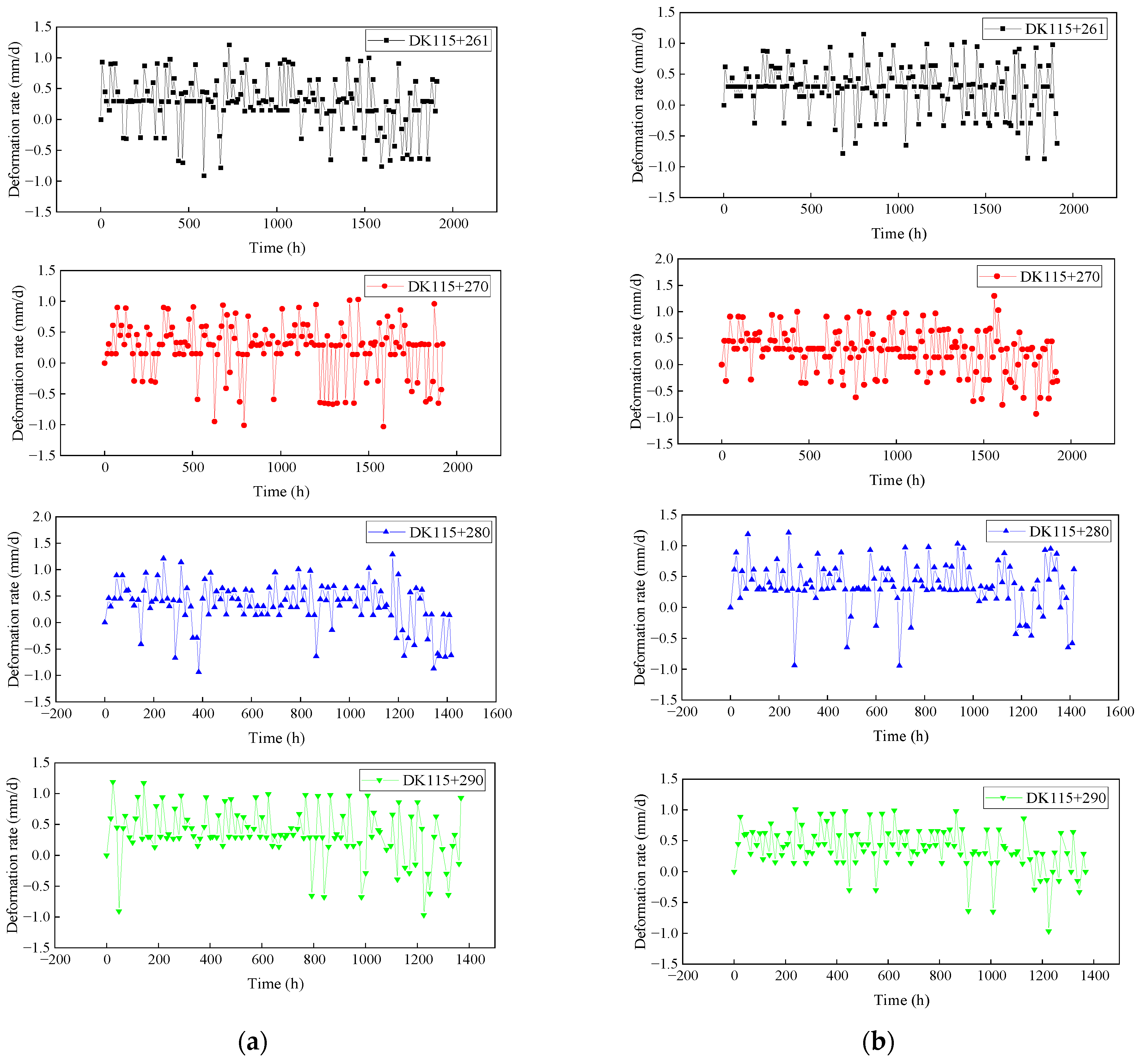
3.1.1. Characterization of Tunnel Deformation Rate Data

Before investigating the multifractal characteristics of the deformation rate of tunnel settlement and convergence, the basic statistical characteristics of the sample data should be understood. Here, the descriptive statistics of the monitoring data in Figure 2 are shown in

Table 1. Descriptive statistics of monitoring data.

Typology	Cross-Section	Average (mm)	Standard Deviation (mm)	Skewness	Kurtosis	J–B Statistic
Tunnel settlement deformation rate	DK115 + 261	0.2611	0.4294	0.5138	0.2869	7.3987
	DK115 + 270	0.2343	0.4292	0.8202	0.6275	20.6918
	DK115 + 280	0.3354	0.4405	0.7564	0.7089	13.7218
	DK115 + 290	0.3454	0.4327	0.7001	0.9317	13.0826
Tunnel convergence deformation rate	DK115 + 261	0.2711	0.3971	0.4901	0.3564	7.0700
	DK115 + 270	0.2509	0.4171	0.3174	0.0704	2.7189
	DK115 + 280	0.3469	0.3950	0.7898	1.5932	24.7456
	DK115 + 290	0.3686	0.3523	0.8295	1.7593	27.0453

.

According to the K–S criterion [59,60], the four evaluation indexes for average, standard deviation, skewness, and kurtosis are considered:

• From the average: the average tunnel deformation rate of each cross-section is greater than 0, which shows positive deformation.
• From the standard deviation: The standard deviation values of the tunnel deformation rate at each cross-section are close. In the deformation rate of tunnel settlement, the standard deviation at DK115 + 280 is the largest, which can be visualized in Figure 2a. In the deformation rate of tunnel convergence, the standard deviation at DK115 + 270 is the largest, which can be visualized in Figure 2b. The standard deviations are all close to or greater than the mean, indicating a greater degree of dispersion in the data.
• From the skewness: The skewness value of each cross-section is greater than 0, indicating that the data distribution is right-skewed. That is, the dispersion on the right side of the mean is stronger than that on the left side, showing a certain degree of long tail on the right side. All skewness values are greater than the mean and standard deviation, indicating a greater degree of skewness in the data distribution.
• From the kurtosis: the kurtosis value for each cross-section is greater than 0, indicating that the peaks of the data are steeper than the peaks of the normal distribution resulting in a spiky state.

In summary, the combined Jarque–Bera (J–B) statistic results are all significantly greater than 0. Under the joint effect of kurtosis and skewness, the deformation rate of each cross-section does not follow a normal distribution. This means that the deformation rate of the tunnel has obvious fractal characteristics, which can be investigated by the relevant methods of fractal theory.

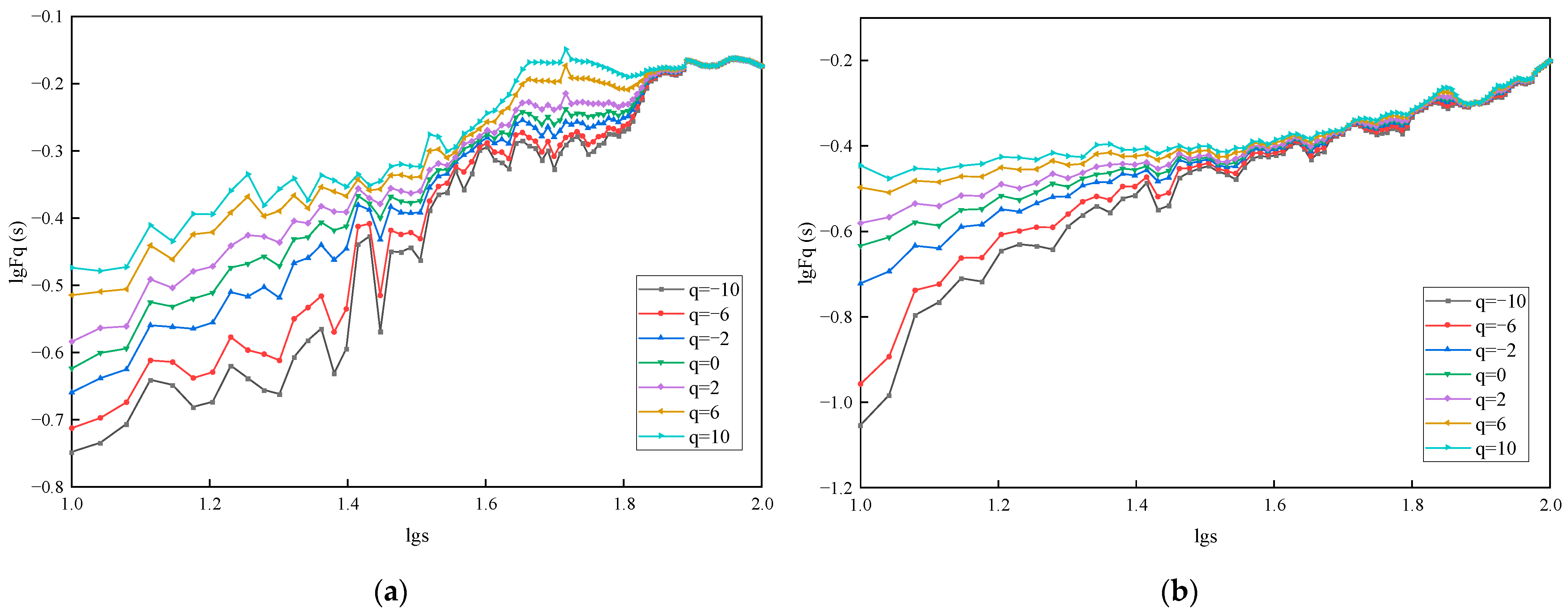
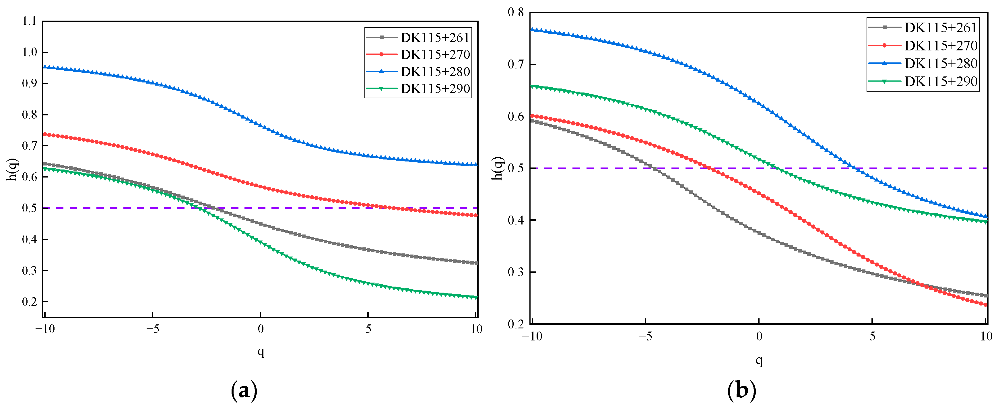
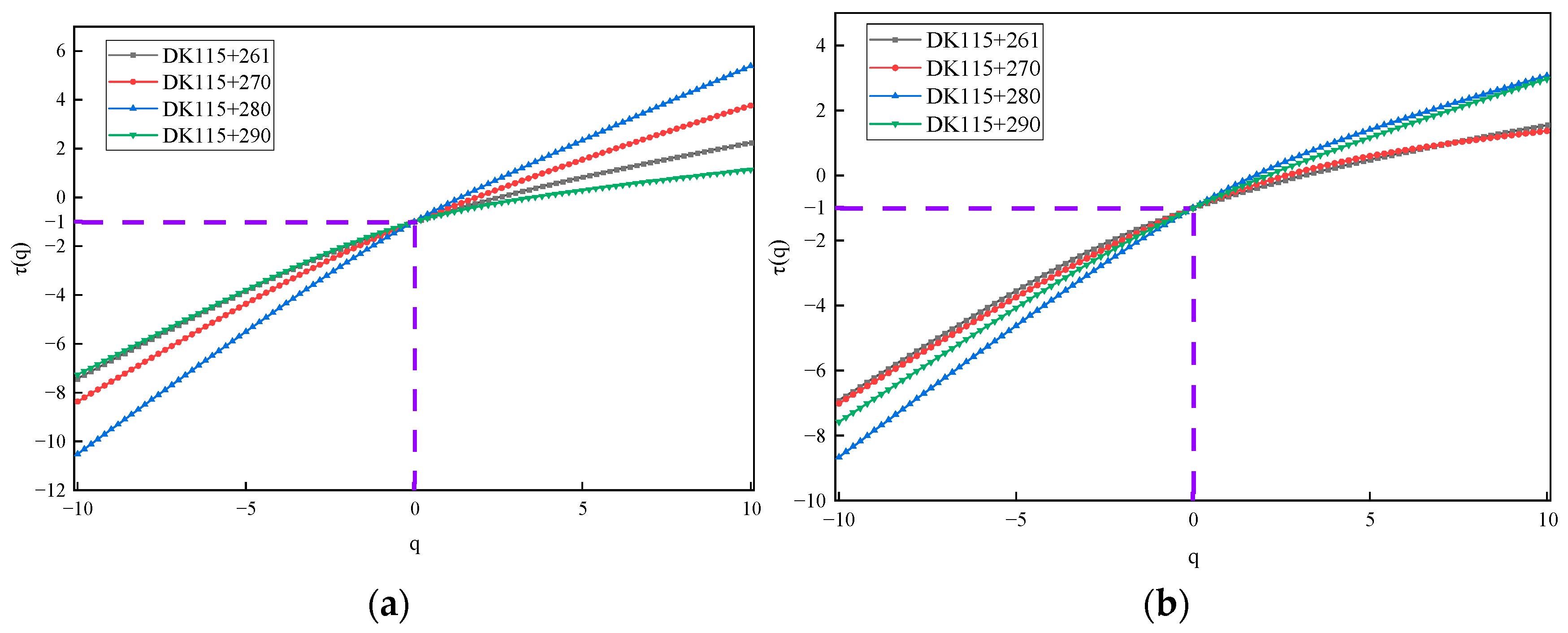
3.1.2. Multifractal Analysis

1.

MF-DFA key parameter settings

The values of the parameters in multifractal theory affect the calculation results in different ways. The features of the non-stationary time series differ significantly in various scenarios, including the length of the signal time window and the fluctuation trend. Therefore, the key parameters need to be tried and predicted to estimate more reliable results.

In order to effectively use multiple fractal theory to analyze the fractal characteristics of the tunnel displacement deformation rate, a double logarithmic scatterplot of $lg{F}_q\left(s\right)-lgs$ is plotted by varying the fluctuation order $q$ ($q$ ∈ [−10, 10]). Least squares fitting was used with the slope of the generalized Hurst exponent $h\left(q\right)$. Taking a set of multifractal features of tunnel settlement deformation rate and tunnel convergence deformation rate as an example, Figure 6 shows the trend of the q-order fluctuation function ${lgF}_q\left(s\right)-lgs$ through double logarithmic fitting.

The curve-fitting for the tunnel section settlement rate in Figure 6a shows better results when the value of lgs ranges from 1.5 to 1.65. At this time, the multifractal time length s is set as smin = 32 and smax = 45.

The curve-fitting for the tunnel section convergence rate in Figure 6b demonstrates improved performance when the value of lgs ranges from 1.1 to 1.4. At this time, the multifractal time length s is set as smin = 13 and smax = 25.

2.

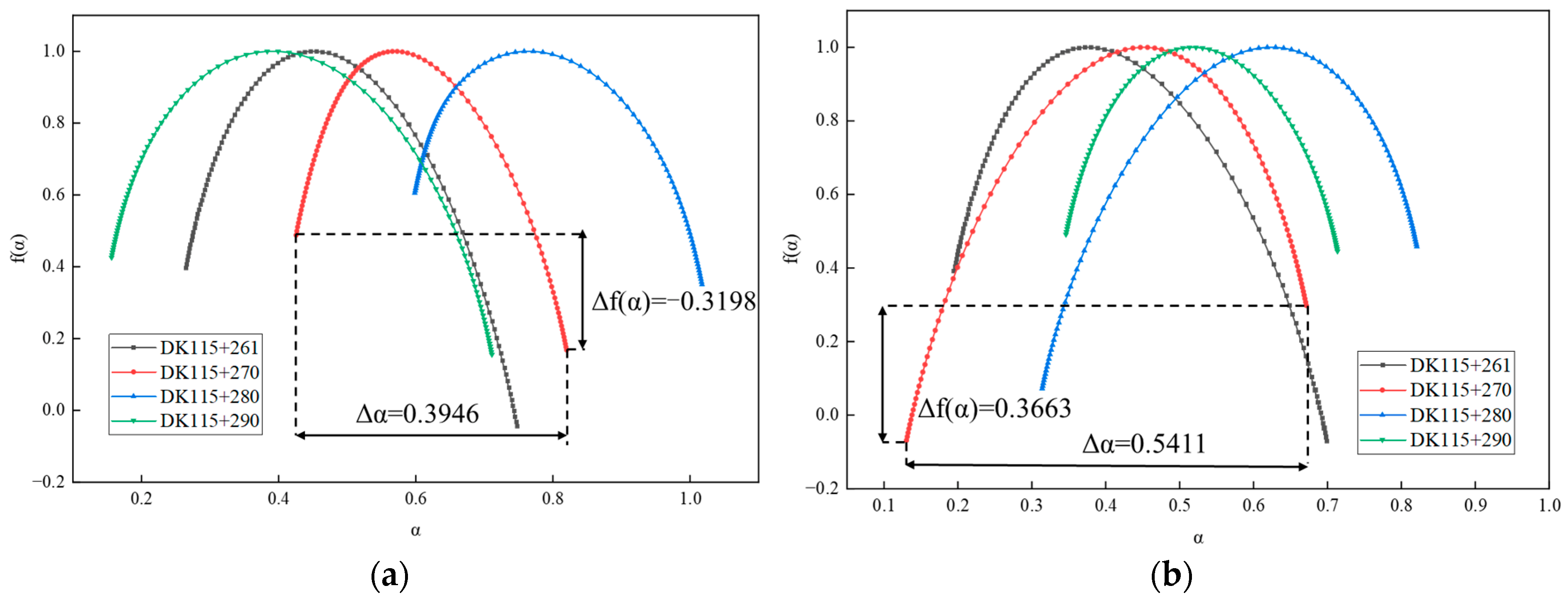
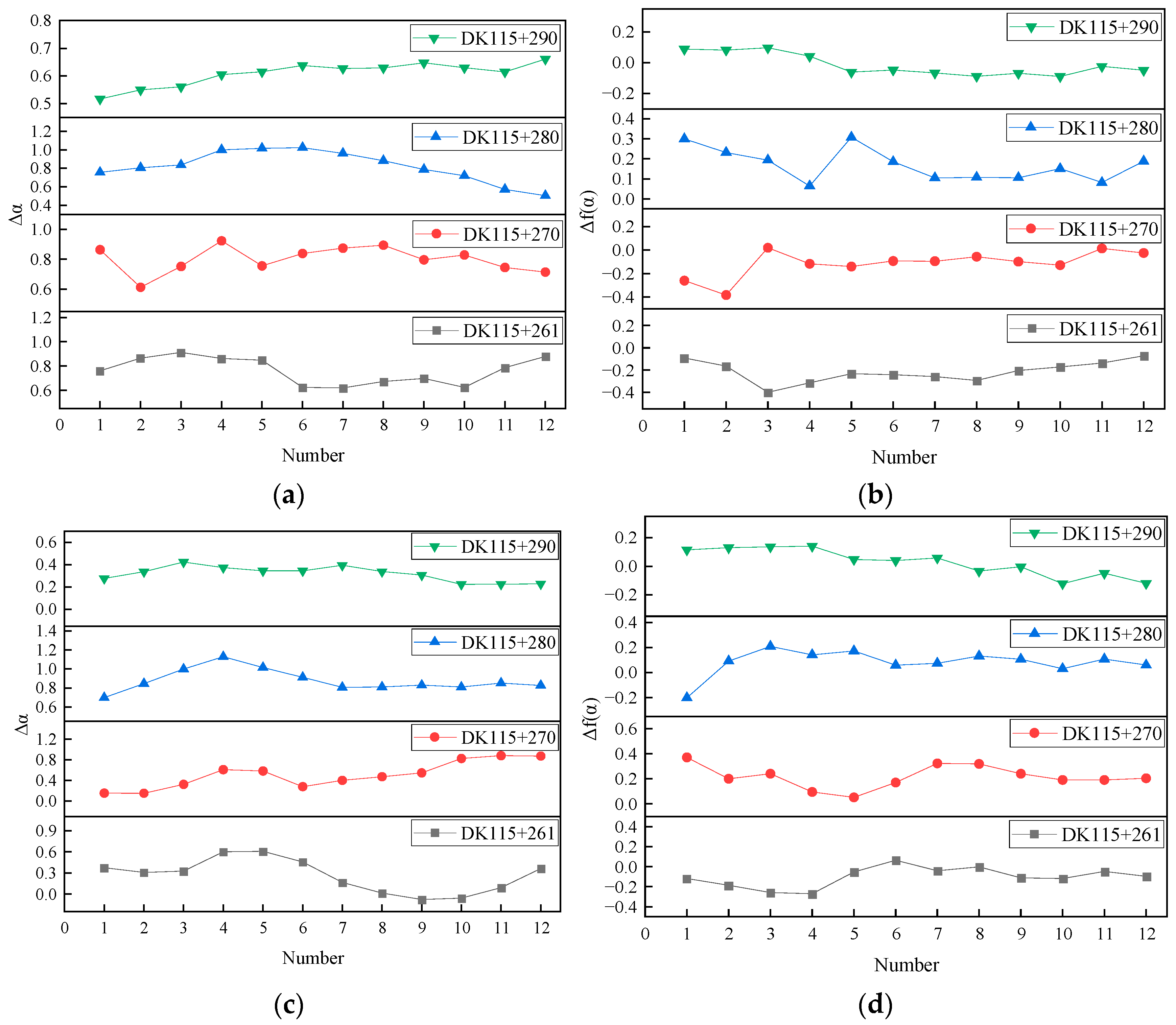
Multifractal characterization of tunnel deformation rates

According to the settings of the above parameters, the data series for tunnel settlement deformation rate and tunnel convergence deformation rate were subjected to multifractals using MATLAB software (R2018b), respectively. The variation of the generalized Hurst index of the tunnel deformation rate data series is shown in Figure 7. The variation of the scalar function $\tau \left(q\right)$ of the tunnel deformation rate data series is shown in Figure 8. The multifractal spectrum of the tunnel deformation rate data series is shown in Figure 9.

As can be seen from Figure 7, as q ranges from −10 to 10, the generalized Hurst index of each section measured data is non-constant. Rather, it exhibits a nonlinear decreasing trend with the change of q, suggesting that the measured data of each cross-section display clear multifractal characteristics. When $h\left(q\right)<0.5$, the data series exhibits a memory process with inverse persistence, while $h\left(q\right)>0.5$ indicates a memory process with positive persistence.

As can be seen from Figure 7a, at different fluctuation orders q, the generalized Hurst exponent curves of tunnel settlement rate at DK115 + 290 are concentrated in the lower fluctuations of the other sections. This indicates a weak multifractal nature.

As can be seen from Figure 7b, at different fluctuation orders q, the generalized Hurst exponent curves of the tunnel convergence rate of DK15 + 261 concentrate in the lower fluctuations of the other sections. This indicates a weak multifractal nature.

On the basis of h(q), the Renyi index, i.e., the scaling function $\tau \left(q\right)$, is calculated. As can be seen from Figure 8, the consistency of the scalar function of the monitoring data of each cross-section is good, and the central part is up-convex, which satisfies $\tau \left(0\right)=-1$. Additionally, there is an overall nonlinear relationship, which further confirms that the monitoring data of each section have multifractal characteristics.

As can be seen from Figure 9, each image of the multifractal spectrum shows a single-peak convex distribution, which resembles a quadratic function curve. The local scales of the multiple fractals of the deformation rate of the tunnel in each section are not constant, reflecting the diversity of local variations at different moments. The singularity intensity $\alpha$ is mainly concentrated on the two sides of the image, reflecting the uneven distribution of the fractal structure of the data series. The uneven distribution of $\alpha$ also confirms the multifractal characteristics of the measured point series; $f\left(\alpha \right)$ characterizes the fractal dimension of the subintervals of the data series with the same singularity index $\alpha$, which is correlated with the distributional characteristics and fractal intensity of the data series. The statistics of the multifractal features of the tunnel settlement rate and tunnel convergence rate measurement data sequences are calculated from Equation (8), as shown in

Table 2. Multifractal characterization statistics.

	Cross-Section	DK115 + 261	DK115 + 270	DK115 + 280	DK115 + 290
Feature
Tunnel settlement rate	$∆\alpha$	0.4829	0.3946	0.4187	0.5547
	$∆f\left(\alpha \right)$	−0.4415	−0.3198	−0.2551	−0.2704
Tunnel convergence rate	$∆\alpha$	0.5042	0.5411	0.5069	0.3674
	$∆f\left(\alpha \right)$	−0.4360	0.3663	0.3860	−0.0455

.

As can be seen from Figure 9a, the fractal spectrum of the tunnel settlement rate measurement data series for each section shows a clear right hook, indicating that the influence of small fluctuations is dominant. The results indicate that the tunnel settlement rate primarily exhibits minor fluctuations throughout the entire monitoring process. During the tunnel construction process, the settlement of the tunnel vault is minimally impacted by excavation and other external influences, remaining within the normal range of settlement changes.

As can be seen from Figure 9b, the sequence fractal spectrum of the tunnel convergence rate measurement data of DK115 + 290 is basically symmetrical, with good overall synergy and a stable development state. The sequence fractal spectrum of the tunnel convergence rate measurement data of DK115 + 261 shows an obvious right hook, indicating that the influence of small fluctuations is dominant. The fractal spectrum of the sequence of the tunnel convergence rate measurement data of DK115 + 270 and DK115 + 280 shows an obvious left hook, indicating that the influence of large fluctuations is dominant.

The fluctuation of the tunnel convergence rate in section DK115 + 290 remains stable throughout the entire monitoring process. During the tunnel construction process, the tunnel convergence in this section is minimally affected by excavation and other external influences, remaining within the normal range of convergence changes. Similarly, in section DK115 + 261, the tunnel convergence rate primarily exhibits minor fluctuations, with the tunnel convergence being less affected by excavation and other external influences, and remaining within the normal range of convergence changes. However, in sections DK115 + 270 and DK115 + 280, the tunnel convergence rate predominantly displays significant fluctuations. During the tunnel construction process in these sections, tunnel convergence is greatly affected by excavation and other external influences, leading to sudden changes. Consequently, it is imperative to reinforce monitoring in these areas.

Comparison of multifractal spectral width ($∆\alpha$). For the tunnel settlement rate measurement data series, the multifractal spectral width $∆\alpha =0.5547$ for DK115 + 290 is the maximum value. It shows that its multifractal intensity is larger, and the fluctuation is more intense and complex. The multifractal spectral width $∆\alpha =0.3946$ of DK115 + 270 is the minimum value. It shows that its multifractal intensity is smaller, and the fluctuation is smoother. For the tunnel convergence rate measurement data series, the multifractal spectrum width $∆\alpha =0.5411$ for DK115 + 270 is the maximum value. It shows that its multifractal intensity is larger, and the fluctuation is more intense and complex. The multifractal spectral width $∆\alpha =0.3674$ of DK115 + 290 is the minimum value. It shows that its multiple fractal intensity is smaller, and the fluctuation is smoother. The results suggest that a larger $∆\alpha$ corresponds to more dramatic and intricate fluctuations, while smaller data changes indicate that tunnel deformation is less affected by external influences such as excavation. Overall, the multiple fractal spectral widths of the measured data series of the tunnel settlement rate and tunnel convergence rate of the same section show an inverse change relationship, and the sum of the two is stable between 0.9 and 1, as shown in Figure 10a.

Compare the proportions of large and small fluctuations ($∆f\left(\alpha \right)$). For the tunnel settlement rate measurement data series, the $∆f\left(\alpha \right)$ in DK115 + 280 is $∆f\left(\alpha \right)=-0.2251$, which is the maximum value. This indicates that the proportion of small fluctuations is larger. The $∆f\left(\alpha \right)$ for DK115 + 261 is $∆f\left(\alpha \right)=-0.4415$, which is the minimum value. This indicates that the proportion of small fluctuations is small. For the tunnel convergence rate measurement data series, the $∆f\left(\alpha \right)$ for DK115 + 280 is $∆f\left(\alpha \right)=0.3663$, which is the maximum value. This indicates that the proportion of small fluctuations is larger. The $∆f\left(\alpha \right)$ for DK115 + 261 is $∆f\left(\alpha \right)=-0.4360$, which is the minimum value. This indicates that the proportion of small fluctuations is small. The findings suggest that a larger $∆f\left(\alpha \right)$ corresponds to small data changes, indicating that tunnel deformation is less affected by external influences such as excavation. Overall, the $∆f\left(\alpha \right)$ in the measured data series of the tunnel settlement rate and tunnel convergence rate of the same section shows the same directional change relationship, as shown in Figure 10b.

3.2. Tunnel Deformation Warning Classification Study

3.2.1. Tunnel Deformation Warning Level Classification Criteria

Based on the research results in the literature [31,61,62], the tunnel displacement monitoring criterion is constructed through the $∆\alpha$ and $∆f\left(\alpha \right)$ parameters derived from the tunnel displacement monitoring data in order to realize the tunnel displacement warning level classification. The specific criteria are set as shown in

Table 3. Tunnel warning level classification criteria.

Warning Level	$∆\mathit{\alpha }$ Indicator Criterion	$∆\mathit{f}\left(\mathit{\alpha }\right)$ Indicator Criterion	Treatment Measures
I	Decreasing trend	Increasing trend	Suspend construction. Use additional temporary support, grouting, and other measures to reinforce the deformed section.
II	Other trend combinations		Conduct a comprehensive evaluation of design and construction measures, reinforce monitoring and measurement protocols, develop disaster prevention plans, and implement appropriate engineering countermeasures when necessary.
III	Steady trend	Steady trend	Normal construction.

.

The trends of the two indicators need to be satisfied at the same time. In case of inconsistency in warning levels, the final warning level is determined according to the most unfavorable principle.

3.2.2. Warning Classification of Tunnel Deformation

The tunnel displacement monitoring data in Figure 4 are used to obtain the required sets of $∆\alpha$ and $∆f\left(\alpha \right)$ parameters. In order to realize the trend judgment of the two discriminant indicators, 100 groups of tunnel displacement monitoring data are divided into one group. Synthesizing the actual situation and monitoring data, a total of 12 groups are divided. Additionally, calculate $∆\alpha$ and $∆f\left(\alpha \right)$ parameters for each group of tunnel displacement monitoring data, as shown in Figure 11.

The trends of the two discriminant indicators were judged using the M–K test to achieve the early warning grading of tunnel displacement. The results are analyzed as follows:

• The analysis of $∆\alpha$ index criterion results: Through calculations and statistical analysis, the results of the $∆\alpha$ index criterion are obtained (see

  Table 4. Results of the ∆α indicator criterion.

  Cross-Section	Section Settlement		Section Convergence
  	Z-Value	Growing Trend	Z-Value	Growing Trend
  DK115 + 261	−1.3540	Steady trend	−2.5849	Decreasing trend
  DK115 + 270	−0.8616	Steady trend	5.0468	Increasing trend
  DK115 + 280	−2.5849	Decreasing trend	−0.8616	Steady trend
  DK115 + 290	5.5391	Increasing trend	−2.8311	Decreasing trend

  ). In the cross-section settlement monitoring data, the Z values for DK115 + 261 and DK115 + 270 fall within the range [−2.32, 2.32], which is a steady trend. The Z value for DK115 + 280 is less than −2.32, which is a decreasing trend. The Z value for DK115 + 290 is more than 2.32, which is an increasing trend. In the cross-section convergence monitoring data, the Z value for DK115 + 280 falls within the range [−2.32, 2.32], which is a steady trend. The Z values for DK115 + 261 and DK115 + 290 are less than −2.32, which is a decreasing trend. The Z value for DK115 + 270 is more than 2.32, which is an increasing trend.
• The analysis of $∆f\left(\alpha \right)$ index criterion results: Through statistical calculations, the results of $∆f\left(\alpha \right)$ index criterion are obtained (see

  Table 5. Results for the $∆f\left(\alpha \right)$ indicator criterion.

  Cross-Section	Section Settlement		Section Convergence
  	Z-Value	Growing Trend	Z-Value	Growing Trend
  DK115 + 261	2.0926	Steady trend	1.6002	Steady trend
  DK115 + 270	2.8311	Increasing trend	−0.3693	Steady trend
  DK115 + 280	−2.5849	Decreasing trend	−0.8616	Steady trend
  DK115 + 290	−4.3082	Decreasing trend	−5.2929	Decreasing trend

  ). In the section settlement monitoring data, the Z value for DK115 + 261 falls between the ranges [−2.32, 2.32], which is a steady trend. The Z value for DK115 + 270 is greater than 2.32, which is an increasing trend. The Z values for DK115 + 280 and DK115 + 290 are less than −2.32, which is a decreasing trend. In the section convergence monitoring data, the Z values for DK115 + 261, DK115 + 270, and DK115 + 280 fall within the range [−2.32, 2.32], which is a steady trend. The Z value for DK115 + 290 is less than −2.32, which is a decreasing trend.
• The analysis of final warning results: On the basis of the results for the $∆\alpha$ indicator criterion and $∆f\left(\alpha \right)$ indicator criterion, the final warning results of the four monitoring cross-sections are analyzed (see

  Table 6. Final warning results of tunnel displacement.

  Cross-Section	DK115 + 261	DK115 + 270	DK115 + 280	DK115 + 290
  Section settlement	III	II	II	II
  Section convergence	II	II	III	II
  Combined warning levels	II	II	II	II

  ). In the section settlement, the warning level for DK115 + 261 is level III, and all other sections are at level II. In section convergence, the warning level of DK115 + 280 is grade III, and all other sections are grade II. Therefore, according to the most unfavorable principle of synthesis, the final warning level of the four sections are all level II. That is, monitoring and measurement should be strengthened, and corresponding engineering countermeasures should be taken if necessary.

3.3. Tunnel Settlement Prediction

3.3.1. Prediction Model Selection

In order to select the tunnel settlement prediction model, the performance of the PSO-LSTM and Back Propagation Neural Network (BP-ANN) prediction models is compared and analyzed. The monitoring data of section DK115 + 261 is used as the sample data to establish the settlement prediction model of PSO-LSTM and BP-ANN. 80% of the data is used as the sample training set, and 20% of the data is allocated to the test set. The delay step of prediction model is set to 6, and the prediction is carried out across 1 time point. The adaptation change curve of PSO-LSTM and BP-ANN are shown in Figure 12.

The tunnel section settlement is predicted, and the prediction results of the two models are compared. The tunnel settlement prediction results for different models are shown in Figure 13. Further, the performance of each model is evaluated using the model evaluation index. The calculation results of the evaluation indexes for the model test set are shown in

Table 7. Results of calculated performance evaluation for the model.

Prediction Model	R2	MAE	RMSE
PSO-LSTM	0.98	0.05	0.06
BP-ANN	0.71	0.16	0.18

. PSO-LSTM predicts significantly better than BP-ANN. Consequently, PSO-LSTM was selected for predicting tunnel settlement data.

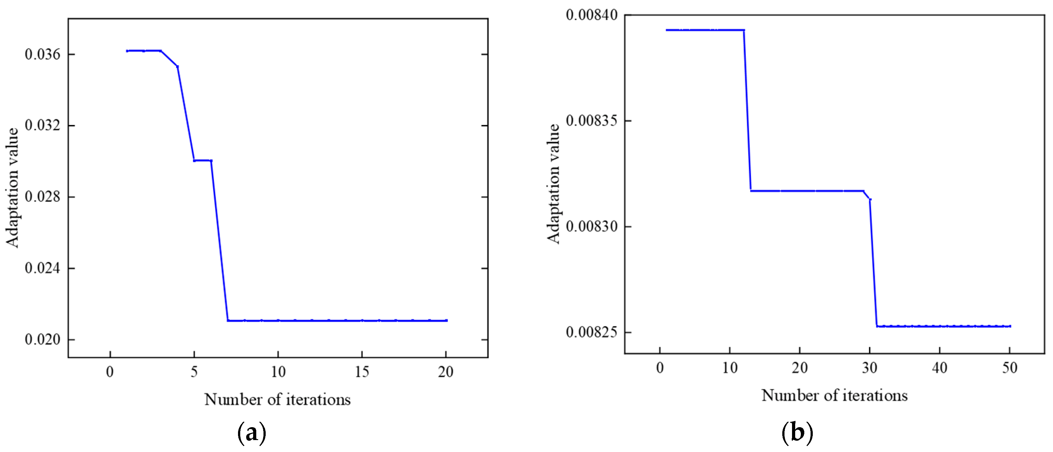
3.3.2. Optimization of PSO-LSTM Parameters

To make the forecast results more concise, subsequent forecasts will be conducted daily. A program was written using Python software (3.9.5) to optimize the parameters of the LSTM prediction model using the PSO algorithm program. The parameters in PSO are set and a range is delineated for the optimization parameters in LSTM: the number of neurons ranges from 10 to 200, the number of training rounds ranges from 10 to 100, and the batch size ranges from 1 to 10. Initialize each parameter of the PSO-LSTM prediction model. Since the total amount of monitoring data is different for each section, after each set of data is input into the PSO program and finishes running, the optimal number of neurons, the number of training rounds, and the batch size of the model are obtained for the 4 groups. The details are shown in

Table 8. PSO-LSTM optimal parameters.

Optimal Parameter	Number of Neurons	Training Rounds	Batch Size
DK115 + 261	77	72	1
DK115 + 270	82	72	1
DK115 + 280	11	99	6
DK115 + 290	20	81	2

.

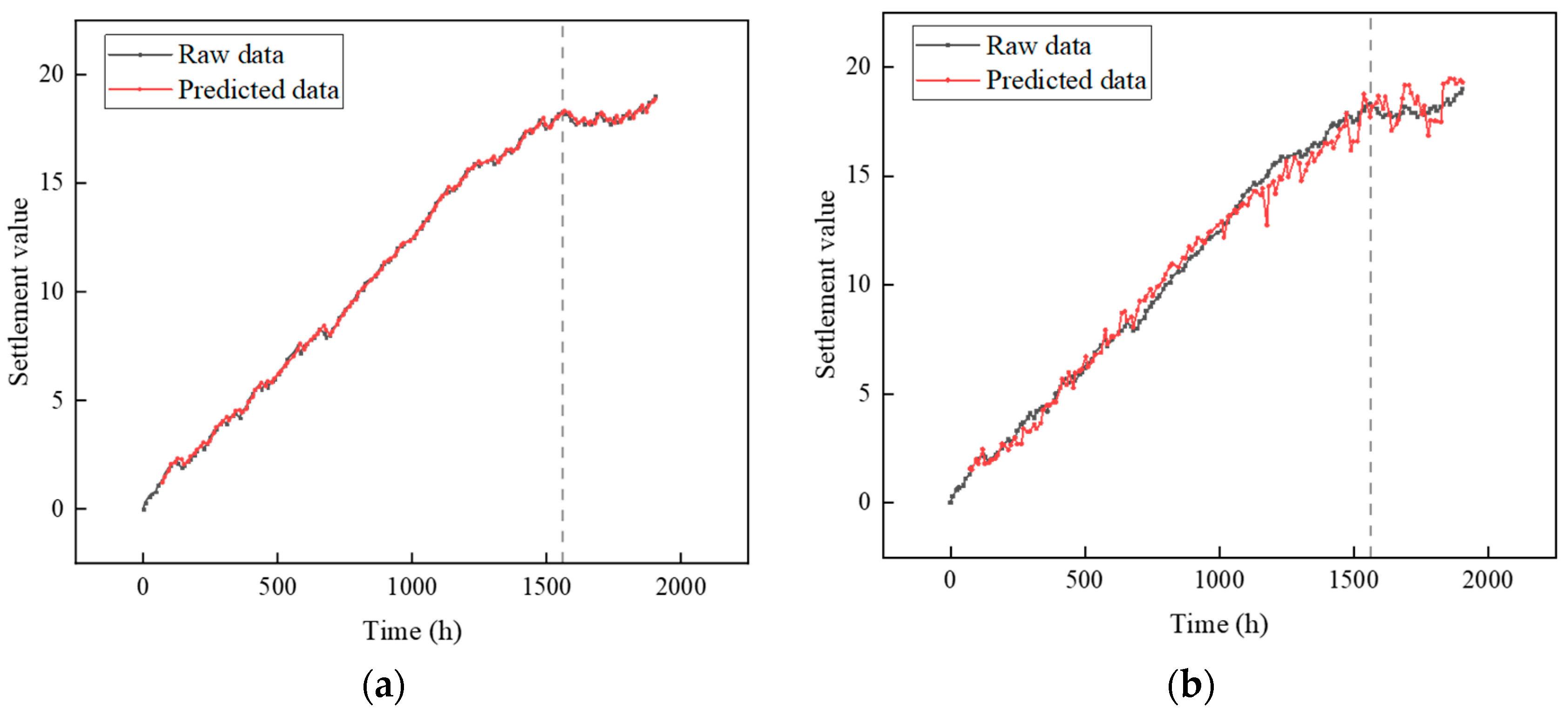
3.3.3. PSO-LSTM Prediction Results

In this study, the PSO-LATM prediction model was constructed using the Python software platform to complete the prediction analysis of cumulative tunnel settlement. The parameters for the LSTM neural network were calculated by PSO. Eighty percent of the data from each section was used as a sample training set and 20% as a test set. R², MAE, and RMSE were used as evaluation indexes for predicting accuracy. Tunnel settlement was predicted for the next 5 days, and the prediction results are shown in

Table 9. Predicted cumulative tunnel settlement values.

Cross-Section	Test Set Evaluation Metrics			Predicted Results
	R2	MAE	RMSE	Day 1	Day 2	Day 3	Day 4	Day 5
DK115 + 261	0.96	0.28	0.06	18.80	18.81	18.81	18.82	18.82
DK115 + 270	0.97	0.10	0.01	18.31	18.32	18.34	18.35	18.36
DK115 + 280	0.98	0.04	0.04	17.50	17.51	17.51	17.51	17.52
DK115 + 290	0.98	0.02	0.02	16.52	16.54	16.55	16.57	16.59

.

For the test set results of settlement prediction for four cross-sections, the test set R² values for the prediction model are 0.96, 0.97, 0.98, and 0.98. The MAE values are 0.28, 0.10, 0.04, and 0.02. The RMSE values are 0.06, 0.01, 0.04, and 0.02. Among these, the closer the R² values for prediction result converge to 1, the smaller the MAE and RMSE become, and the higher the model prediction accuracy is. Therefore, the settlement prediction results of the PSO-LSTM settlement prediction model for the four sections are analyzed. The model’s predictions for the tunnel section settlement are in good agreement with the measured data.

Analyzing the prediction results, the future settlements of the four sections generally show a slowly increasing trend. The accuracy of tunnel warning classification is further verified, and, based on the evaluation indexes, the PSO-LSTM model demonstrates high accuracy in predicting tunnel settlement.

4. Conclusions

In this study, the multifractal theory was utilized to the analyze tunnel deformation, and the sliding time window was employed to enhance the segmentation of traditional multifractal subintervals. Furthermore, the M–K analysis method was utilized to ascertain the multifractal feature trends and establish the warning level for the tunnel section. Subsequently, the accuracy of the warning level was validated by predicting tunnel settlement using the PSO-LSTM prediction model. The following conclusions were drawn:

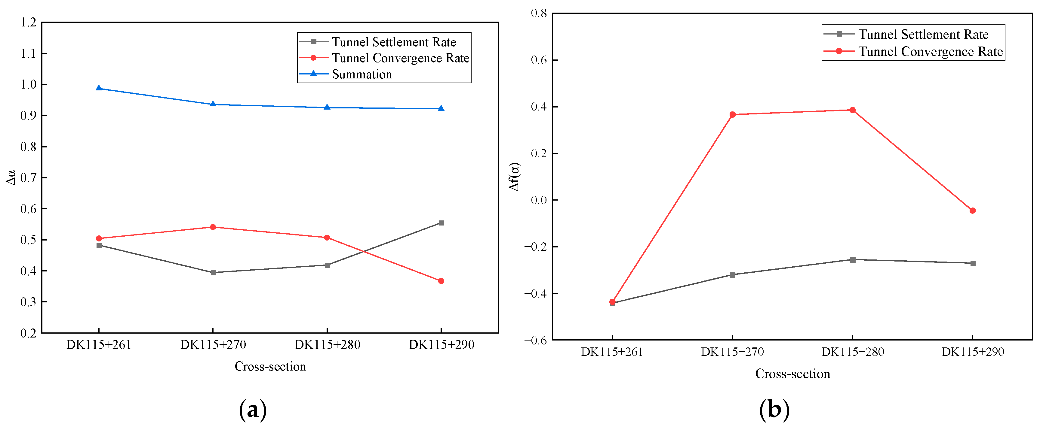
• The tunnel settlement and convergence rates of the four sections exhibit distinct fractal sequence characteristics. The width of the multifractal spectra in the measured data series of tunnel settlement rate and tunnel convergence rate within the same section shows an inverse relationship, with the sum of the two remaining stable between 0.9 and 1. Additionally, the proportion of size fluctuations in the measured data series of the tunnel settlement rate and the tunnel convergence rate within the same section demonstrate a consistent trend.
• The analysis of tunnel settlement prediction indicates that the PSO-LSTM prediction model delivers superior predictive performance and stability in tunnel settlement forecasts.
• A comprehensive analysis of the tunnel warning level and tunnel settlement prediction results reveals a class II tunnel deformation warning level, which aligns with the actual tunnel conditions. This approach, leveraging quantitative data as a reference, enables a more precise determination of the tunnel warning level.

References

1. Liu, C.; Liu, Y.; Chen, Y.; Zhao, C.; Qiu, J.; Wu, D.; Liu, T.; Fan, H.; Qin, Y.; Tang, K. A State-of-the-Practice Review of Three-Dimensional Laser Scanning Technology for Tunnel Distress Monitoring. J. Perform. Constr. Facil. 2023, 37, 03123001. [Google Scholar] [CrossRef]
2. Cao, Y.; Zhang, Z.; Cheng, F.; Su, S. Trajectory Optimization for High-Speed Trains via a Mixed Integer Linear Programming Approach. IEEE Trans. Intell. Transp. Syst. 2022, 23, 17666–17676. [Google Scholar] [CrossRef]
3. Zhao, T. Research on Invert Heave Mechanism and Control Technique of High-speed Railway Tunnel in Mudstone. Ph.D. Thesis, Lanzhou Jiaotong University, Lanzhou, China, 2022. [Google Scholar]
4. Chen, H.; Lai, H.; Qiu, Y.; Chen, R. Reinforcing Distressed Lining Structure of Highway Tunnel with Bonded Steel Plates: Case Study. J. Perform. Constr. Facil. 2020, 34, 04019082. [Google Scholar] [CrossRef]
5. Li, Z.; Lai, J.; Ren, Z.; Shi, Y.; Kong, X. Failure mechanical behaviors and prevention methods of shaft lining in China. Eng. Fail. Anal. 2023, 143, 106904. [Google Scholar] [CrossRef]
6. Weng, X.; Li, H.; Hu, J.; Li, L.; Xu, L. Behavior of Saturated Remolded Loess Subjected to Coupled Change of the Magnitude and Direction of Principal Stress. Int. J. Géoméch. 2023, 23, 04022244. [Google Scholar] [CrossRef]
7. Wang, Z.; Cai, Y.; Fang, Y.; Lai, J.; Han, H.; Liu, J.; Lei, H.; Kong, X. Local buckling characteristic of hollow π-type steel-concrete composite support in hilly-gully region of loess tunnel. Eng. Fail. Anal. 2023, 143, 106828. [Google Scholar] [CrossRef]
8. Zhou, M.; Fang, Q.; Peng, C. A mortar segment-to-segment contact method for stabilized total-Lagrangian smoothed particle hydrodynamics. Appl. Math. Model. 2022, 107, 20–38. [Google Scholar] [CrossRef]
9. Zhen, Y.; Guo, P.; Wang, L.; Chen, X.; Duan, X.; Wang, A. Key Technologies for Treating High Ground Stress and Large Deformation of Soft Rock in Daliangshan Tunnel of Yunlin Expressway. Tunn. Constr. Available online: https://link.cnki.net/urlid/44.1745.U.20231107.1430.003 (accessed on 8 November 2023).
10. Zhang, C.; Han, K.; Zhang, D. Face stability analysis of shallow circular tunnels in cohesive-frictional soils. Tunn. Undergr. Space Technol. 2015, 50, 345–357. [Google Scholar] [CrossRef]
11. Li, W.; Zhang, C.; Zhang, D.; Ye, Z.; Tan, Z. Face stability of shield tunnels considering a kinematically admissible velocity field of soil arching. J. Rock Mech. Geotech. Eng. 2021, 14, 505–526. [Google Scholar] [CrossRef]
12. Li, G.; Hu, Y.; Tian, S.-M.; Weibin, M.; Huang, H.-L. Analysis of deformation control mechanism of prestressed anchor on jointed soft rock in large cross-section tunnel. Bull. Eng. Geol. Environ. 2021, 80, 9089–9103. [Google Scholar] [CrossRef]
13. Wu, H.-N.; Shen, S.-L.; Chen, R.-P.; Zhou, A. Three-dimensional numerical modelling on localised leakage in segmental lining of shield tunnels. Comput. Geotech. 2020, 122, 103549. [Google Scholar] [CrossRef]
14. Shen, S.-L.; Wu, H.-N.; Cui, Y.-J.; Yin, Z.-Y. Long-term settlement behaviour of metro tunnels in the soft deposits of Shanghai. Tunn. Undergr. Space Technol. 2014, 40, 309–323. [Google Scholar] [CrossRef]
15. Lai, H.; Zhao, X.; Kang, Z.; Chen, R. A new method for predicting ground settlement caused by twin-tunneling under-crossing an existing tunnel. Environ. Earth Sci. 2017, 76, 726. [Google Scholar] [CrossRef]
16. Suwansawat, S.; Einstein, H.H. Describing settlement troughs over twin tunnels using a superposition technique. Geotech. Geoenviron. Eng. 2007, 133, 445–468. [Google Scholar] [CrossRef]
17. Chou, W.I.; Bobet, A. Predictions of ground deformations in shallow tunnels in clay. Tunn. Undergr. Space Technol. 2002, 17, 3–19. [Google Scholar] [CrossRef]
18. Zhang, J.-Z.; Huang, H.-W.; Zhang, D.-M.; Phoon, K.K.; Liu, Z.-Q.; Tang, C. Quantitative evaluation of geological uncertainty and its influence on tunnel structural performance using improved coupled Markov chain. Acta Geotech. 2021, 16, 3709–3724. [Google Scholar] [CrossRef]
19. Li, Y.; Li, J.; Zhao, J.; Zhao, T.; Guo, D. Research on a Safety Evaluation System for Railway-Tunnel Structures by Fuzzy Comprehensive Evaluation Theory. Civ. Eng. J.-Staveb. Obz. 2023, 32, 122–136. [Google Scholar] [CrossRef]
20. Li, Z.; Meng, X.; Liu, D.; Tang, Y.; Chen, T. Disaster Risk Evaluation of Superlong Highways Tunnel Based on the Cloud and AHP Model. Adv. Civ. Eng. 2022, 2022, 8785030. [Google Scholar] [CrossRef]
21. Yan, X.; Li, H.; Liu, F.; Liu, Y. Structural Safety Evaluation of Tunnel Based on the Dynamic Monitoring Data during Construction. Shock Vib. 2021, 2021, 6680675. [Google Scholar] [CrossRef]
22. Tan, X.; Chen, W.; Zou, T.; Yang, J.; Du, B. Real-time prediction of mechanical behaviors of underwater shield tunnel structure using machine learning method based on structural health monitoring data. J. Rock Mech. Geotech. Eng. 2023, 15, 886–895. [Google Scholar] [CrossRef]
23. Tang, L.; Na, S. Comparison of machine learning methods for ground settlement prediction with different tunneling datasets. J. Rock Mech. Geotech. Eng. 2021, 13, 1274–1289. [Google Scholar] [CrossRef]
24. Zhang, W.; Li, Y.; Wu, C.; Li, H.; Goh, A.; Liu, H. Prediction of lining response for twin tunnels constructed in anisotropic clay using machine learning techniques. Undergr. Space 2022, 7, 122–133. [Google Scholar] [CrossRef]
25. Suwansawat, S.; Einstein, H.H. Artificial neural networks for predicting the maximum surface settlement caused by EPB shield tunneling. Tunn. Undergr. Space Technol. 2006, 21, 133–150. [Google Scholar] [CrossRef]
26. Yang, H.; Song, K.; Zhou, J. Automated Recognition Model of Geomechanical Information Based on Operational Data of Tunneling Boring Machines. Rock Mech. Rock Eng. 2022, 55, 1499–1516. [Google Scholar] [CrossRef]
27. Schappacher, N. Mandelbrot, Benoît B. The Fractal Geometry of Nature. In Kindlers Literatur Lexikon (KLL); WH Freeman: New York, NY, USA, 2020; pp. 1–2. [Google Scholar]
28. Zuo, C.; Liu, D.; Ding, S.; Li, L. Analysis and Prediction of Tunnel Surface Subsidence Based on Fractal Theory. J. Yangtze River Sci. Res. Inst. 2016, 33, 51–56. [Google Scholar] [CrossRef]
29. Ye, D.; Liu, G.; Tian, Y.; Sun, Z.; Yu, B. A Fractal Model for the Micro–Macro Interactions on Tunnel Leakage. Fractals 2022, 30, 2250142. [Google Scholar] [CrossRef]
30. Grassberger, P. Generalized dimensions of strange attractors. Phys. Lett. A 1983, 97, 227–230. [Google Scholar] [CrossRef]
31. Lei, H.; Zhou, X.; Wang, Y. Research on Landslide Early Warning and Prediction Based on Combined Response of Multifractal Characteristics and Sub Item Prediction. J. Geod. Geodyn. 2022, 42, 885–891. [Google Scholar]
32. Mao, H.; Zhang, M.; Jiang, R.; Li, B.; Xu, J.; Xu, N. Study on deformation pre-warning of rock slopes based on multi-fractal characteristics of microseismic signals. Chin. J. Rock Mech. Eng. 2020, 39, 560–571. [Google Scholar]
33. Zhou, L.; Liu, Z. Multifractal feature analysis method for measured data of dam deformation. Adv. Sci. Technol. Water Resour. 2021, 41, 18–24. [Google Scholar] [CrossRef]
34. Hughes, H.M. The relative cuttability of coal-measures stone. Min. Sci. Technol. 1986, 3, 95–109. [Google Scholar] [CrossRef]
35. Hamidi, J.K.; Shahriar, K.; Rezai, B.; Rostami, J. Performance prediction of hard rock TBM using Rock Mass Rating (RMR) system. Tunn. Undergr. Space Technol. 2010, 25, 333–345. [Google Scholar] [CrossRef]
36. Goh, A.T.C.; Zhang, W.; Zhang, Y.; Xiao, Y.; Xiang, Y. Determination of earth pressure balance tunnel-related maximum surface settlement: A multivariate adaptive regression splines approach. Bull. Eng. Geol. Environ. 2018, 77, 489–500. [Google Scholar] [CrossRef]
37. Ozdemir, L. Development of Theoretical Equations for Predicting Tunnel Boreability. Ph.D. Thesis, Colorado School of Mines, Golden, CO, USA, 1977. [Google Scholar]
38. Resendiz, D.; Romo, M.P. Settlements upon soft-ground tunneling: Theoretical solution. Int. J. Rock Mech. Min. Sci. Geomech. Abstr. 1983, 151, 65–74. [Google Scholar]
39. Bai, B. Fluctuation responses of saturated porous media subjected to cyclic thermal loading. Comput. Geotech. 2006, 33, 396–403. [Google Scholar] [CrossRef]
40. Bai, B.; Nie, Q.; Zhang, Y.; Wang, X.; Hu, W. Cotransport of heavy metals and SiO2 particles at different temperatures by seepage. J. Hydrol. 2020, 597, 125771. [Google Scholar] [CrossRef]
41. Rowe, R.K.; Lee, K.M. Subsidence owing to tunnelling. II. Evaluation of a prediction technique. Can. Geotech. J. 1992, 29, 941–954. [Google Scholar] [CrossRef]
42. Yuan, B.; Li, Z.; Su, Z.; Luo, Q.; Chen, M.; Zhao, Z. Sensitivity of Multistage Fill Slope Based on Finite Element Model. Adv. Civ. Eng. 2021, 2021, 6622936. [Google Scholar] [CrossRef]
43. Yuan, B.; Li, Z.; Zhao, Z.; Ni, H.; Su, Z.; Li, Z. Experimental study of displacement field of layered soils surrounding laterally loaded pile based on transparent soil. J. Soils Sediments 2021, 21, 3072–3083. [Google Scholar] [CrossRef]
44. Yuan, B.; Li, Z.; Chen, Y.; Ni, H.; Zhao, Z.; Chen, W.; Zhao, J. Mechanical and microstructural properties of recycling granite residual soil reinforced with glass fiber and liquid-modified polyvinyl alcohol polymer. Chemosphere 2021, 286, 131652. [Google Scholar] [CrossRef]
45. Chou, J.; Lin, C. Predicting Disputes in Public-Private Partnership Projects: Classification and Ensemble Models. J. Comput. Civ. Eng. 2013, 27, 51–60. [Google Scholar] [CrossRef]
46. Bouayad, D.; Emeriault, F. Modeling the relationship between ground surface settlements induced by shield tunneling and the operational and geological parameters based on the hybrid PCA/ANFIS method. Tunn. Undergr. Space Technol. 2017, 68, 142–152. [Google Scholar] [CrossRef]
47. Santos, O.J.; Celestino, T.B. Artificial neural networks analysis of Sao Paulo subway tunnel settlement data. Tunn. Undergr. Space Technol. 2008, 23, 481–491. [Google Scholar] [CrossRef]
48. Hasanipanah, M.; Noorian-Bidgoli, M.; Armaghani, D.J.; Khamesi, H. Feasibility of PSO-ANN model for predicting surface settlement caused by tunneling. Eng. Comput. 2016, 32, 705–715. [Google Scholar] [CrossRef]
49. Chen, Y.; Zhao, B.; Wang, H.; Zheng, J.; Gao, Y. Time-Series InSAR Ground Deformation Prediction Based an LSTM Model. Yangtze River. Available online: https://link.cnki.net/urlid/42.1202.TV.20231117.0949.002 (accessed on 17 November 2023).
50. Li, C.; Li, J.; Shi, Z.; Li, L.; Li, M.; Jin, D.; Dong, G. Prediction of Surface Settlement Induced by Large-Diameter Shield Tunneling Based on Machine-Learning Algorithms. Geofluids 2022, 2022, 4174768. [Google Scholar] [CrossRef]
51. Cao, Y.; Zhou, X.; Yan, K. Deep Learning Neural Network Model for Tunnel Ground Surface Settlement Prediction Based on Sensor Data. Math. Probl. Eng. 2021, 2021, 9488892. [Google Scholar] [CrossRef]
52. Duan, C.; Hu, M.; Zhang, H. Comparison of ARIMA and LSTM in Predicting Structural Deformation of Tunnels during Operation Period. Data 2023, 8, 104. [Google Scholar] [CrossRef]
53. Mann, H.B. Nonparametric Tests Against Trend. Econometrica 1945, 13, 245–259. [Google Scholar] [CrossRef]
54. Kendall, M.G.; Gibbons, J.D. Rank Correlation Method. Biometrika. 1990. Available online: http://www.jstor.org/stable/2333282 (accessed on 18 June 2014).
55. Wang, L.I.; Gao, X.; Zhou, W. Testing for Intrinsic Multifractality in the Global Grain Spot Market Indices: A Multifractal Detrended Fluctuation Analysis. Fractals 2023, 31, 2350090. [Google Scholar] [CrossRef]
56. Wang, F.; Shao, W.; Yu, H.; Kan, G.; He, X.; Zhang, D.; Ren, M.; Wang, G. Re-evaluation of the Power of the Mann-Kendall Test for Detecting Monotonic Trends in Hydrometeorological Time Series. Front. Earth Sci. 2020, 8, 14. [Google Scholar] [CrossRef]
57. Hochreiter, S.T.U.M.; Schmidhuber, J. Long short-term memory. Neural Comput. 2010, 9, 1735–1780. [Google Scholar] [CrossRef] [PubMed]
58. Kennedy, J.; Eberhart, R. Particle Swarm Optimization. In Proceedings of the ICNN’95-International Conference on Neural Networks, Perth, WA, Australia, 27 November–1 December 1995. [Google Scholar]
59. Wu, Z. Time-Varying Risk Aversion and Crude Oil Futures Price Volatility. Master’s Thesis, Anhui University of Finance & Economics, Bengbu, China, 2023. [Google Scholar]
60. Xie, W. Study on the Interdependence Structure and Risk Spillover Effect between Cryptocurrency and Chinese financial Assets. Ph.D. Thesis, Nanjing University of Information Science & Technology, Nanjing, China, 2023. [Google Scholar]
61. Guo, Y.; Zheng, J.; Liu, H. An early warning method for tunneling-induced ground surface settlement considering accident precursors and consequences. Tunn. Undergr. Space Technol. 2023, 140, 105214. [Google Scholar] [CrossRef]
62. Wang, J.; Wang, X. Early Warning and Prediction of Side Displacement and Deformation of Soft Soil Foundation Pit. J. Yangtze River Sci. Res. Inst. 2021, 38, 91–96. [Google Scholar]
Figure 1. Flow chart of tunnel deformation analysis and early warning prediction.
Fractalfract 08 00108 g001
Figure 2. Tunnel section.
Fractalfract 08 00108 g002
Figure 3. Tunnel deformation monitoring and measurement: (a) tunnel monitoring point layout, (b) manual monitoring and measurement.
Fractalfract 08 00108 g003
Figure 4. Tunnel cumulative deformation–time diagrams: (a) tunnel cumulative settlement–time diagram, (b) tunnel cumulative convergence–time diagram.
Fractalfract 08 00108 g004
Figure 5. Tunnel deformation rate–time diagrams: (a) tunnel settlement rate–time diagram, (b) tunnel convergence rate–time diagram.
Fractalfract 08 00108 g005
Figure 6. Trend plot of q-order fluctuation function l g F q ( s ) l g s double logarithmic fit: (a) settlement rate of section DK115 + 261, (b) convergence rate of section DK115 + 261.
Fractalfract 08 00108 g006
Figure 7. Variation of generalized Hurst index: (a) tunnel settlement rate; (b) tunnel convergence rate.
Fractalfract 08 00108 g007
Figure 8. Variation of the scalar function τ(q): (a) tunnel settlement rate; (b) tunnel convergence rate.
Fractalfract 08 00108 g008
Figure 9. Multifractal spectrum: (a) tunnel settling rate; (b) tunnel convergence rate.
Fractalfract 08 00108 g009
Figure 10. Plot of multifractal feature statistics: (a) multifractal spectral width α ; (b) proportion of size fluctuations f ( α ) .
Fractalfract 08 00108 g010
Figure 11. Calculated values of α and f ( α ) parameters: (a) α parameter values for tunnel settlement, (b) f ( α ) parameter values for tunnel settlement, (c) α parameter values for tunnel convergence, (d) f ( α ) parameter values for tunnel convergence.
Fractalfract 08 00108 g011
Figure 12. Adaptation change curves for different prediction models: (a) PSO-LSTM adaptation change curve; (b) BP-ANN adaptation change curve.
Fractalfract 08 00108 g012
Figure 13. Tunnel settlement prediction results for different prediction models: (a) PSO-LSTM prediction results; (b) BP-ANN prediction results.
Fractalfract 08 00108 g013