The El Niño Southern Oscillation Recharge Oscillator with the Stochastic Forcing of Long-Term Memory

Abstract

The influence of the fast-varying variables that have a long-term memory on the El Niño Southern Oscillation (ENSO) is investigated by adding a fractional Ornstein–Uhlenbeck (FOU) process stochastic noise on the simple recharge oscillator (RO) model. The FOU process noise converges to zero very slowly with a negative power law. The corresponding non-zero ensemble mean during the integration period can exert a pronounced influence on the ensemble-mean dynamics of the RO model. The state-dependent noise, also called the multiplicative noise, can present its influence by reducing the relaxation coefficient and by introducing periodic external forcing. The decreasing relaxation coefficient can enhance the oscillation amplitude and shorten the oscillation period. The forced frequency is close to the natural frequency. The two mechanisms together can further amplify the amplitude and shorten the period, compared with the state-independent noise or additive noise, which only exhibits its influence by introducing non-periodic external forcing. These two mechanisms explicitly elucidate the influence of the stochastic forcing on the ensemble-mean dynamics of the RO model. It provides comprehensive knowledge to better understand the interaction between the fast-varying stochastic forcing and the slow-varying deterministic system and deserves further investigation.

1. Introduction

The El Ni$\tilde{\mathrm{n}}$o Southern Oscillation (ENSO) phenomenon is generated by a complex atmosphere–ocean coupling mechanism and is characterized by SST anomalies (SSTAs) that fluctuate significantly on a large scale in the tropical Pacific [1]. ENSO has been considered to exert significant and profound influences on changes in the regional weather and even global climate patterns [2]. Therefore, the fundamental dynamics of ENSO have been extensively investigated. Generally speaking, the ENSO cycle is controlled by positive feedback and negative feedback. This feedback determines the SSTA variations that can affect the trade wind, and hence the oceanic motion, which can further affect SSTA variation, in turn. The Bjerknes positive feedback emphasized that a warm SSTA in the eastern Pacific can weaken the trade wind, then reduce the oceanic upwelling, and then further amplify the warm SSTA there, and vice versa. There are two classic negative mechanisms. For example, a delayed oscillator model for ENSO is established to highlight the oceanic wave transit effect by introducing negative, delayed feedback [3,4]. A recharge oscillator (RO) model is constructed to emphasize the recharge–discharge of the equatorial heat content as the phase-transition mechanism [5]. Recently, a spatiotemporal oscillator model was proposed to characterize the complex temporal and spatial variations in ENSO [6]. These studies considered ENSO as a slow deterministic oscillation of the atmosphere-ocean interaction. However, in fast atmospheric synoptic–intraseasonal variations, such as the Madden–Julian Oscillation (MJO) [7,8,9,10,11], the westerly wind bursts (WWBs) [12,13,14,15,16] may also have a significant influence on the variability and prediction of ENSO. This synoptic–intraseasonal variability, the source of the noise in the tropics, can be regarded as a stochastic forcing of ENSO [17].

Specific to the RO framework, the random wind stress forcing and random heating forcing can be added into SSTA and the thermocline depth anomaly (TDA) dynamics [18,19,20]. For mathematical convenience, these random forcings are represented by the Langevin equation with a constant damping coefficient, that is, the Ornstein–Uhlenbeck (OU) process. The results suggest that the stochastic forcing can change the growth rate to enhance ENSO activity in the RO model. Moreover, the stochastic forcing can increase the ensemble spread and thus may reduce the effectiveness of the prediction of ENSO. However, the OU process is a Gaussian process with zero ensemble mean and exponential auto-correlation function, which denotes a short-term memory. It might not be a better prototype of the real world, where the auto-correlation functions of variables might be power functions, denoting a long-term memory [21,22].

Considering the fact that the ensemble-mean dynamics of the RO model under stochastic forcing with a short-term memory have been intensively investigated [18,19,20], we may explore the performance of stochastic forcing with a long-term memory. As an analog, the fractional OU (FOU) process that has a long-term memory [23,24,25] is a natural choice. Then, the influence mechanism of the FOU process of stochastic forcing on the ensemble-mean dynamics of the RO model, and the differences from the previous OU process stochastic forcing results [18], become the key scientific questions. Therefore, this paper attempts to answer these questions by applying a simple RO model [26] under the stochastic forcing of the FOU process. The investigation will be beneficial in allowing an in-depth understanding of the interaction between the fast-varying stochastic forcing and the slow-varying deterministic RO model.

Following this introduction section, the simple RO model forced by the FOU process forcing is presented in Section 2. The analytic solution of the FOU process is also discussed. The ensemble-mean dynamics of the RO model forced by stochastic forcing are derived and analyzed in Section 3. Finally, a conclusion and discussion end the paper in Section 4.

2. The Model Framework

Previous studies [18,19,20] have added multiplicative noise forcing onto the simple conceptual RO model to describe the influence of the fast atmospheric fluctuations that associate with the MJO/WWB activity. This theoretical framework has the following form:

$$\left\{\begin{array}{l}\frac{\mathrm{d}T}{\mathrm{d}t}=-\lambda T+\omega h+\sigma \xi \left(t\right)G\\ \frac{\mathrm{d}h}{\mathrm{d}t}=-\omega T\\ \mathrm{d}\xi =-r\xi \mathrm{d}t+\mathrm{d}W\left(t\right)\end{array}\right.,$$

(1)

where $T$ and $h$ are the sea surface temperature anomaly (SSTA) in the eastern Pacific and the thermocline depth anomaly (TDA), respectively. $\lambda$ is the relaxation of SSTA toward climatology. $\omega$ denotes the thermocline upwelling process. $\sigma$ is the noise amplitude. $\xi \left(t\right)$ is a stochastic process. $W\left(t\right)$ is a standard Brownian motion (or the Wiener process), and its increment $\mathrm{d}W$ is the Gaussian white noise. $r>0$ is a constant damping coefficient. $G=1+BT$ represents the state-dependent noise forcing due to the interannual modulation of WWB/MJO activity via SSTAs. Particularly, if $G=1$ (or $B=0$), then the system is forced by the additive noise, which is state-independent. The first two equations in Equation (1) represent the simple RO model with a stochastic forcing. The third equation in Equation (1) is the OU Langevin equation.

As Jin et al. [18] suggested, the stochastic forcing term $\sigma \xi \left(t\right)G$ represents the effects of the fast atmospheric wind anomalies (short de-correlation timescales). However, as stated previously, the fast atmospheric anomalies might own a long-term memory that cannot be expressed by the stochastic OU process. To take the long-term memory into consideration, a simple approach is to generalize the OU process to a fractional one; that is,

$$\mathrm{d}\xi =-r\xi \mathrm{d}t+\mathrm{d}{W}^{\alpha }\left(t\right),$$

(2)

where $W^{\alpha }\left(t\right)$ is a fractional Brownian motion, and its increment $\mathrm{d}{W}^{\alpha }$ can be called a fractional Gaussian noise. Here, the superscript $\alpha$ ($0<\alpha <1$) denotes the derivative order. Note that the FOU process Equation (2) has the same form as the OU process but with different type of noise (they will be the same if $\alpha =1$). Therefore, it can be called a fractional Langevin equation. According to [27], the fractional derivative ${\xi }^{\left(\alpha \right)}$ of order $\alpha$ satisfies the usual OU process; that is,

$$\mathrm{d}{\xi }^{\left(\alpha \right)}=-r{\xi }^{\left(\alpha \right)}\mathrm{d}t+\mathrm{d}W\left(t\right),$$

(3)

and its solution is

$${\xi }^{\left(\alpha \right)}={\xi }_0^{\left(0\right)}{e}^{-rt}+{\displaystyle {\int }_0^t{e}^{r\left(s-t\right)}}\mathrm{d}W\left(s\right),$$

(4)

where ${\xi }_0^{\left(\alpha \right)}={\xi }^{\left(\alpha \right)}\left(0\right)$ is the initial value. Here, the Caputo-type derivative is adopted; that is,

$${\xi }^{\left(\alpha \right)}\triangleq {}_0{}^{C}D_t^{\alpha }\xi \left(t\right)=\frac{1}{\Gamma \left(1-\alpha \right)}{\displaystyle {\int }_0^t{\left(t-\tau \right)}^{-\alpha }{\xi }^{\prime }\left(\tau \right)d\tau },$$

(5)

where ${\xi }^{\prime }\left(t\right)$ is the first derivative. Applying the fractional integral of order $\alpha$, we can derive the solution of Equation (2):

$$\xi \left(t\right)={\xi }_0^{\left(\alpha \right)}{E}_t\left(\alpha ,-r\right)+\frac{1}{\Gamma \left(1+\alpha \right)}{\displaystyle {\int }_0^t{\left(t-\tau \right)}^{\alpha }{\displaystyle {\int }_0^{\tau }{e}^{s-\tau }}\mathrm{d}W\left(s\right)d\tau },$$

(6)

where $E_t\left(\alpha ,-r\right)=\frac{{\left(-r\right)}^{-\alpha }{e}^{-rt}\gamma \left(\alpha ,-r\right)}{\Gamma \left(\alpha \right)}=t^{\alpha }{E}_{1,\alpha +1}\left(-rt\right)$ is the Et function, and $\gamma \left(\alpha ,-r\right)$ is a lower incomplete gamma function; $E_{\alpha ,\beta }\triangleq {\displaystyle \sum _{k=0}^{\infty }\frac{z^k}{\Gamma \left(\alpha k+\beta \right)}}$ is the Mittag–Leffler function [28]. Although the analytic solution can be derived, it introduces an extra parameter that is not easy to specify. Therefore, we may just propose an alternative equation for Equation (2) or Equation (3) by replacing the first derivative of $\xi \left(t\right)$ with a fractional derivative of an order $\alpha$. It can be written as

$${\mathrm{d}}^{\left(\alpha \right)}\xi \left(t\right)=-r\xi \mathrm{d}t+\mathrm{d}W,$$

(7)

and its solution [29] is

$$\xi \left(t\right)={\xi }_0{E}_{\alpha ,1}\left(-r{t}^{\alpha }\right)+{\displaystyle {\int }_0^t{\left(t-s\right)}^{\alpha -1}{E}_{\alpha ,\alpha }\left[-r{\left(t-s\right)}^{\alpha }\right]dW\left(s\right)}$$

(8)

where ${\xi }_0=\xi \left(0\right)$ is the initial value. Compared with Equation (6), it only needs the initial value of the stochastic process. Moreover, if $\alpha =1$, then Equation (7) will reduce to the standard OU process. We still call Equation (7) an FOU process for convenience.

Replacing the third equation in Equation (1) with Equation (7), the RO model with the fractional stochastic forcing becomes

$$\left\{\begin{array}{l}\frac{\mathrm{d}T}{\mathrm{d}t}=-\lambda T+\omega h+\sigma \xi \left(t\right)G\\ \frac{\mathrm{d}h}{\mathrm{d}t}=-\omega T\\ {\mathrm{d}}^{\left(\alpha \right)}\xi =-r\xi \mathrm{d}t+\mathrm{d}W\end{array}\right.$$

(9)

Equation (9) is the theoretical framework that this investigation applies. Since we mainly emphasize the influence of stochastic forcing with long-term memory, we do not introduce the seasonal cycle in this investigation. It can be easily conducted to set the seasonal varying relaxation coefficient $\lambda ={\lambda }_0+{\lambda }_{ac}\cos \left({\omega }_{ac}t-\varphi \right)$, where ${\omega }_{ac}$, $\varphi$, and ${\lambda }_{ac}$ are the frequency, phase, and amplitude of the annual cycle, respectively.

3. Results

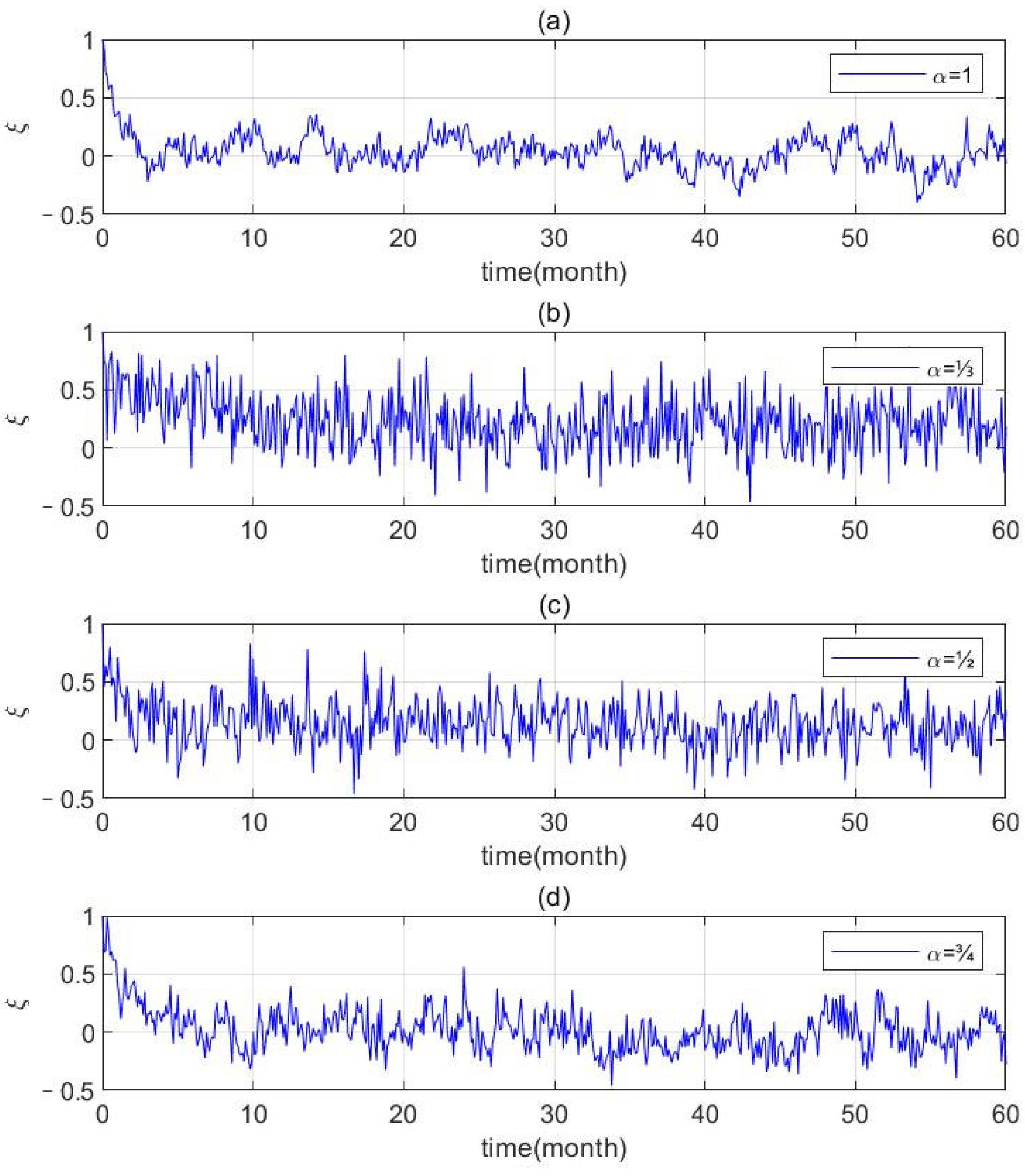
3.1. The Stochastic Forcing of Long-Term Memory

The only difference between this investigation and previous studies is the introduction of the fractional stochastic forcing. Therefore, it is necessary to firstly compare the two types of stochastic forcings. As shown in Figure 1, there is a significant discrepancy between them. For the OU process (Figure 1a), the stochastic noise basically declines exponentially at the beginning time, during which the influence of the Gaussian white noise is relatively weak and the system is mainly determined by its deterministic damping rate. The stochastic noise begins to oscillate around the steady state (zero value, since the exponential law declines toward zero rapidly) with a continuously increasing time, so that the Gaussian white noise begins to exhibit its influence.

For the FOU process (Figure 1b–d), the stochastic noise represents a more pronounced oscillation, characterized by a wider amplitude range and general larger amplitudes. Furthermore, the smaller the fractional order, the more significant the oscillation. For example, the significant decay range at the beginning time may even become implicit (Figure 1b) when $\alpha =1/3$. Moreover, there are marked differences in the probability distribution functions (PDFs) between those two types of noise sequences (Figure 2). For the OU process, the maximum probability exhibits a peak at the value of zero and decreases when the values are far away from zero. Actually, this PDF is a standard normal distribution, since the time is long enough that the exponential decay signal at the beginning can be neglected and the OU process can be regarded as Brownian motion. For the FOU process, in contrast, the maximum probability is not located on the value of zero but a positive increment. The smaller the fractional order becomes, the larger the increment will be. This can be interpreted via the solution in Equation (8) or Equation (6), the first part of which denotes a deterministic damping between the stretched exponential and the negative power law. The former has a very fast decay, while the latter has a very slow decay for a large time [30]. Therefore, even though it tends to be zero when the time tends to be infinity, it does have a relatively large value when the time is large. In the integration time range that is long enough for the RO model, the stochastic process shows a heavy tail, denoting the long-term memory. Thus, it can be predicted that compared with the original OU process, the FOU stochastic noise will bring markable change to the RO model.

3.2. The Influence of FOU Process on the RO Model

Following Jin et al. [18], the parameter values are approximately set to $\lambda =1/6$ month⁻¹, $\omega =2\pi /48$ month⁻¹, $r=1/1.5$ month⁻¹, $\sigma =1/\sqrt{24}$ month⁻¹, and the values of the initial system state are set as $T=0$, $h=2$. According to a recent study [31], the values of RO parameters can be improved by objectively optimizing the RO equations fit to observations.

For the additive noise case ($B=0$), the ensemble-mean solution of the linear RO model shows the dependence on the stochastic forcing (Figure 3). The numerical ensemble-mean SSTA obtained from a 5000-member ensemble (Figure 3a) suggests that the FOU process noise forcing can amplify the amplitude. This is totally different from the OU process stochastic forcing, which is indistinguishable from the deterministic solution with the same initial conditions but without stochastic forcing, according to Jin et al. [18]. Compared with the deterministic SSTA amplitude (or the OU process noise), the SSTA amplitude forced by the FOU process noise can increase by around 15% compared with the initial value. The smaller the fractional derivative order, the larger the strength that the amplitude can approach. The situation for TDA (Figure 3b) is quite similar. The ensemble-mean curves do not represent a complete ENSO cycle due to the positive relaxation coefficient $\mathsf{\lambda }$.

For the multiplicative noise case ($B=1$), the ensemble-mean solution shows similar variations to the previous additive case but with a more significant oscillation amplitude (Figure 4). The SSTA (Figure 4a) can increase to exceed 1.5 °C within eight months, with an increase of around 50% (compared with the initial value) in the case of $\alpha =1/3$, far larger than the increase of around 10% in the case of $\alpha =1$, the corresponding OU-process multiplicative noise. Then, the SSTA declines to around 0.35 °C within around 34 months in the case of $\alpha =1/3$ and to around −0.16 °C within around 37 months in the case of $\alpha =1$. It can be seen that this phase transition time has been advanced for around 3 months. Similar to SSTA variations, TDA (Figure 4b) also exhibits a significantly amplified amplitude and earlier phase transition time in the case of FOU process noise.

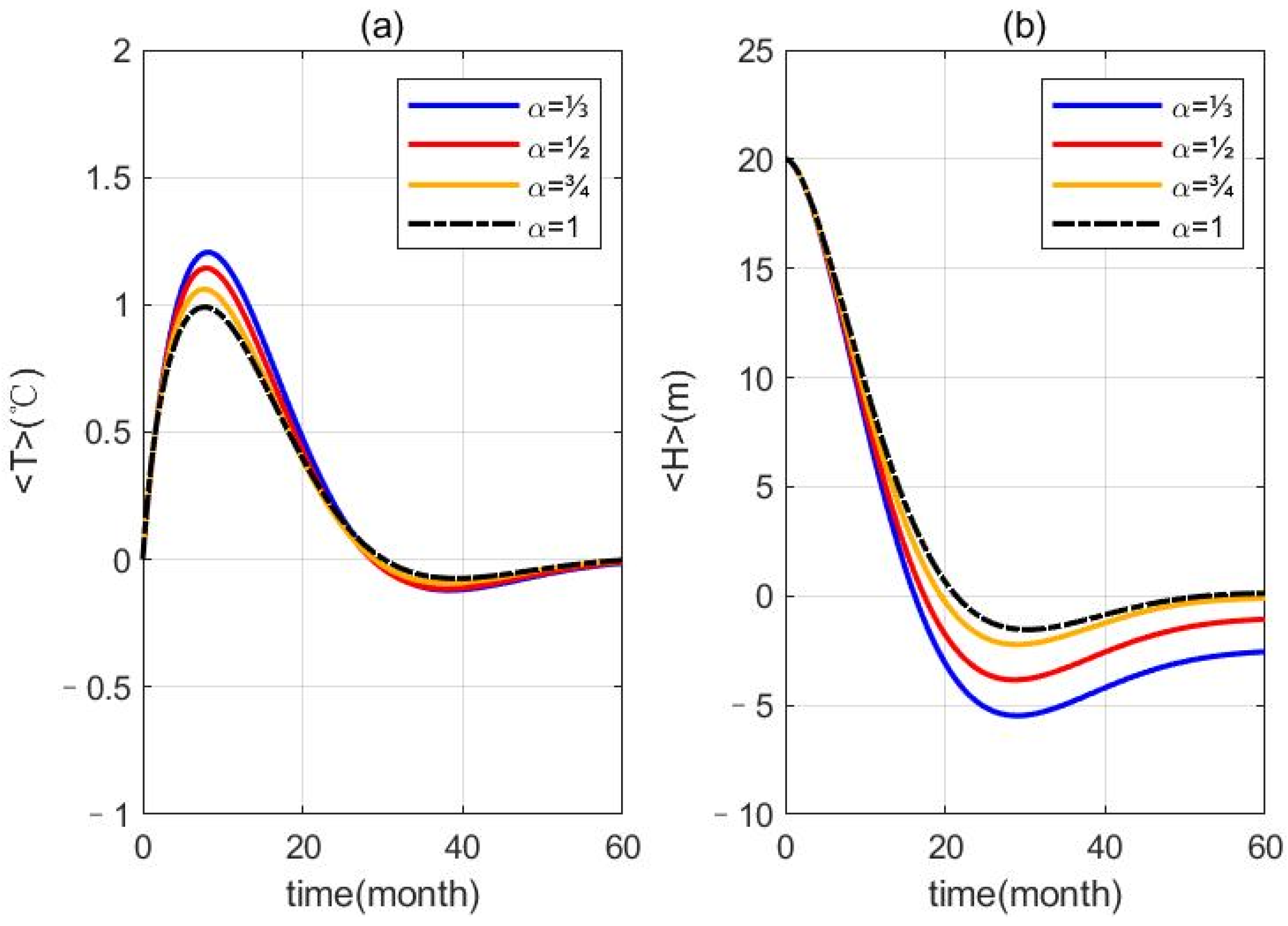
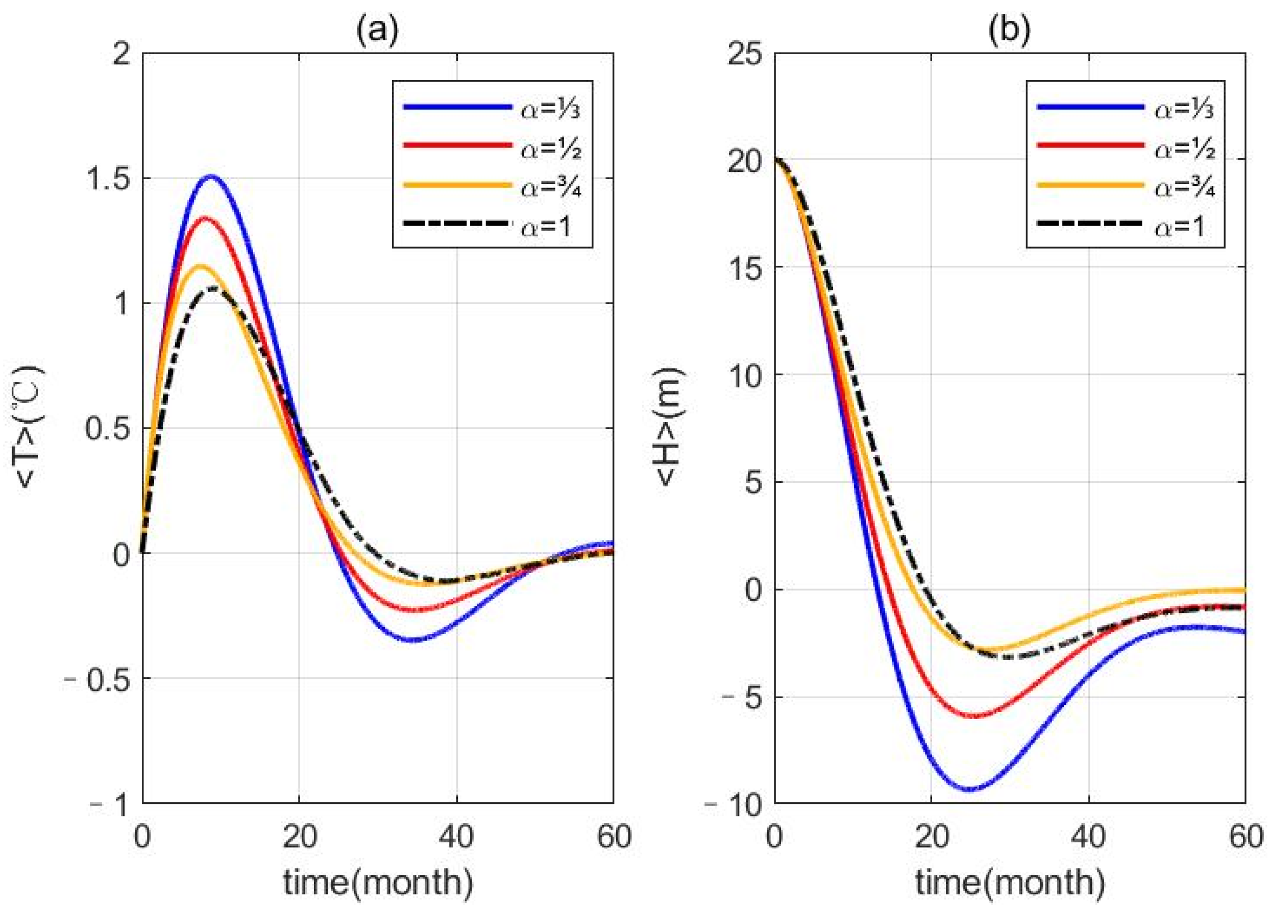
3.3. The Ensemble-Mean Dynamics

It becomes obvious that the FOU process forcing in both additive and multiplicative cases has a significant influence on the amplitude of SSTA and TDA in the ensemble-mean sense. It means that the stochastic forcing, no matter whether it is state-dependent or not, can affect the ensemble-mean state of ENSO. To interpret this phenomenon, let us discuss the ensemble-mean dynamics by separating the variables into the ensemble mean and the departure, namely, $T=〈T〉+T^{\prime }$ and $h=〈h〉+h^{\prime }$, where $〈T〉$ and $〈h〉$ are the ensemble means for $T$ and $h$ and $T^{\prime }$ and $h^{\prime }$ denote the departures, respectively. The ensemble-mean equations for the RO model are

$$\left\{\begin{array}{l}\frac{\mathrm{d}〈T〉}{\mathrm{d}t}=-\lambda 〈T〉+\omega 〈h〉+\sigma 〈\xi 〉\left(1+B〈T〉\right)+\sigma B〈\xi T^{\prime }〉\\ \frac{\mathrm{d}〈h〉}{\mathrm{d}t}=-\omega 〈T〉\end{array}\right..$$

(10)

The third term on the right-hand side in the first equation of Equation (10) is associated with the ensemble mean for the stochastic process. The ensemble mean for the OU process converges rapidly (exponential law) to zero so that it can be neglected. However, according to Equation (6) or Equation (8) the ensemble mean for the FOU process converges slowly (negative power law) to zero so that it can manifest its influence during the integration time period. In reality, the ensemble mean determined by the first term on the right-hand side of Equation (6) or Equation (8) has an asymptotic representation $f\left(\alpha \right)t^{-\alpha }$ when $t\to \infty$, where $f\left(\alpha \right)$ is a bounded function [30]. Therefore, we may set the ensemble mean for the FOU process $〈\xi 〉\sim t^{-\alpha }$. This means that even if we only consider an additive noise ($B=0$), as an external forcing, it will still exert its influence on the ensemble-mean states. Furthermore, its influence will be more significant at the beginning time when $〈\xi 〉$ has a relatively large value. This is totally different from the previous investigations [18,19,20], which suggested that the additive OU process noise had no effect on the ensemble-mean dynamics. Strictly, the additive OU process noise also plays a role, which decreases rapidly to zero. Now we know that whether a stochastic process can exert influence on the ensemble-mean dynamics or not depends on the evolution of its ensemble mean. For a stochastic process, such as the OU process, it has little effect on the ensemble-mean dynamics, since its ensemble mean converges to zero very rapidly. For a stochastic process, such as the FOU process that this investigation applies, it can affect the ensemble-mean dynamics due to its slowly convergent ensemble mean. Of course, its influence will be insignificant when the time is very large.

The situation will be more complex if we consider the multiplicative noise, which means that the ensemble mean for $〈\xi T^{\prime }〉$ should be considered. Since it will be inconvenient when we apply the fractional derivative form of the FOU process (Equation (7)), we turn to its first derivative form (Equation (2)) to derive the ensemble-mean equations:

$$\left\{\begin{array}{l}\frac{\mathrm{d}〈\xi T^{\prime }〉}{\mathrm{d}t}=-\left(\lambda +r+〈\xi 〉\sigma B\right)〈\xi T^{\prime }〉+\omega 〈\xi h^{\prime }〉+\sigma B〈{\xi }^2{T}^{\prime }〉\\ \frac{\mathrm{d}〈\xi h^{\prime }〉}{\mathrm{d}t}=-r〈\xi h^{\prime }〉-\omega 〈\xi T^{\prime }〉\end{array}\right..$$

(11)

Ignoring the higher-order term $〈{\xi }^2{T}^{\prime }〉$, the system can be enclosed and it has the same form of the RO model. We can easily derive its solution if we assume that $〈\xi 〉$ is independent of time. It is

$$〈\xi T^{\prime }〉=e^{-\frac{1}{2}{\lambda }_{+}t}\left(A_1\cos {\omega }_{2}t+A_2\sin {\omega }_{2}t\right),$$

(12)

where ${\lambda }_{+}=\left(\lambda +〈\xi 〉\sigma B\right)$, ${\omega }_2=\frac{1}{2}\sqrt{4{\omega }^2-{\lambda }_{+}^2}$, $A_1$, and $A_2$ are constants. Supposing $〈\xi 〉>0$, we can find out that the oscillation frequency ${\omega }_2<{\omega }_0=\frac{1}{2}\sqrt{4{\omega }^2-{\lambda }^2}$, the frequency of the RO model. Meanwhile, the damping coefficient ${\lambda }_{+}>\lambda$, the relaxation coefficient of the RO model. This means that the multiplicative noise will introduce a slower and stronger decayed oscillation to force the RO model. With increasing time, $〈\xi 〉$ will be smaller and smaller and tend toward zero. It will lead ${\lambda }_{+}\approx \lambda$ and hence ${\omega }_2\approx {\omega }_0$, that is, the first order term $〈\xi T^{\prime }〉$ has the same frequency as the RO model. Moreover, the larger the $\sigma B$, the more significant the influence that the stochastic process can exert.

Substituting Equation (12) into Equation (10), the ensemble-mean equations can finally be written as

$$\left\{\begin{array}{l}\frac{\mathrm{d}〈T〉}{\mathrm{d}t}=-{\lambda }_{-}〈T〉+\omega 〈h〉+g\left(t\right)\\ \frac{\mathrm{d}〈h〉}{\mathrm{d}t}=-\omega 〈T〉\end{array}\right.$$

(13)

where ${\lambda }_{-}=\lambda -〈\xi 〉\sigma B$, $g\left(t\right)=\sigma 〈\xi 〉+\sigma B{e}^{-{\lambda }_{+}t}\left(A_1\cos {\omega }_{2}t+A_2\sin {\omega }_{2}t\right)$. And its solution is

$$〈T〉=e^{-\frac{1}{2}{\lambda }_{-}t}\left(C_1\cos {\omega }_{1}t+C_2\sin {\omega }_{1}t\right)+{〈T〉}^{*}$$

(14)

where ${\omega }_1=\frac{1}{2}\sqrt{4{\omega }^2-{\lambda }_{-}^2}$, $C_1$, and $C_2$ are constants; ${〈T〉}^{*}$ is the special solution determined by $g\left(t\right)$. Similarly, we can find out that ${\omega }_1>{\omega }_0$ and ${\lambda }_{-}<\lambda$, denoting a natural oscillation with higher frequency and weaker damping. It provides a theoretical explanation for previous calculation results, as Figure 4 portrays. Note that the special solution has a frequency ${\omega }_2$, which is close to the frequency of the RO model (${\omega }_0$) and also close to the frequency of the ensemble-mean oscillation (${\omega }_1$), namely, ${\omega }_2\le {\omega }_0\le {\omega }_1$. Furthermore, we may assume that ${\omega }_1\approx {\omega }_0+\delta$ and ${\omega }_2\approx {\omega }_0-\delta$, where $\delta$ is a small positive frequency increment. Now, let us consider a simple case, where

$$〈T〉\sim \sin {\omega }_{1}t+\sin {\omega }_{2}t,$$

(15)

in which the natural oscillation and the forced oscillation have the same amplitude. Equation (15) can be rearranged as

$$〈T〉\sim \sin {\omega }_{0}t\cos \delta t.$$

(16)

It is clear that the ensemble-mean SSTA oscillation will show a wave train shape. The $\sin {\omega }_{0}t$ part is the carrier wave, denoting the phase propagation. The $\cos \delta t$ part is the wave packet, the envelop line of the carrier wave, denoting the amplitude propagation. Due to the fact that the relaxation coefficient is positive and the ensemble mean for stochastic forcing converges to zero, the ensemble-mean SSTA is a decayed oscillation. Therefore, we do not observe the wave train feature in Figure 4.

4. Conclusions and Discussion

To investigate the influence of fast atmospheric activities that may have a long-term memory on ENSO, we introduce stochastic forcing with long-term memory that is represented by an FOU process in a simple conceptual RO model. The FOU process shows quite different features compared with those of the OU process. The process decreases to zero very slowly with a negative power law when the time is large. During a long integration period that is long enough for the RO model, the FOU process forcing does not converge to zero rapidly like the Gaussian OU process. Therefore, the FOU process noise seems to have a non-zero mean value in the integration period.

This new feature can significantly influence the ensemble-mean dynamics of the simple RO model. The additive noise can exert is influence through introducing a non-periodic external forcing that obeys the negative power law. The external forcing can enhance the oscillation amplitude but has little effect on the oscillation period, which can be seen from Figure 3. The multiplicative noise plays its role by reducing the relaxation coefficient and by introducing a periodic external forcing, which is solved using the second-order enclosed ensemble-mean RO equations. The frequency of the periodic forcing is higher than, and close to, the frequency of the first-order enclosed ensemble-mean RO model. The two close frequencies can cause the ensemble-mean SSTA oscillation to present a wave train shape. On the other hand, a decreasing relaxation coefficient can strengthen the oscillation amplitude. Moreover, a decreasing relaxation coefficient can increase the oscillation frequency, denoting a faster oscillation. With these two mechanisms, the multiplicative noise can exert a more significant influence on the ensemble-mean dynamics than the additive noise, which can be clearly seen from Figure 3 and Figure 4.

The finding that both additive and multiplicative noise can affect the ensemble-mean dynamics of ENSO further develops the previous knowledge that emphasized the importance of the multiplicative noise and deemed additive noise ineffective. Therefore, we may conclude that there is no essential discrepancy between the FOU process additive and multiplicative noises, although there is indeed a difference in the degree of impact.

Stochastic noises with long-term memory present extensively in nature. The simple RO framework forced by FOU-process stochastic noise can be further extended to consider more physical processes. The ensemble spread can also be discussed by applying the enclosed ensemble-mean equations. Therefore, continuous explorations may be beneficial for not only deeply understanding the influence of the fast atmospheric activities on slow ENSO variations, but also reducing the ensemble spread and improving the predictability.

ENSO is the most dominant interannual signal, but not the only signal. To improve our physical understanding of internal climate variability across the global oceans, a conceptual model hierarchy that consists of the classic stochastic climate model formulated by Klaus Hasselmann, the classic RO model, and the effect of the seasonal cycle on both of these models can be also proposed to capture the essence of observed SST variability from sub-seasonal to decadal timescales [32,33]. Under this model framework, the classic RO model is just a building block, only contributing to the deterministic interannual variability (labelled as $T_{ENSO}$). The total interannual SSTA variability (labelled as $T$) is also affected by a damping term and a stochastic forcing term, the classic Hasselmann climate model. Moreover, the seasonable cycle can be introduced to both the damping term and the RO model. Although this stochastic–deterministic model is different from the theoretical framework that this investigation applies, there is indeed linkage between them. The stochastic–deterministic model can be seen as an extension of the classic stochastic Hasselmann climate model, which is driven by deterministic interannual oscillation, seasonable cycles, and stochastic noise. The RO framework with stochastic noise also means that ENSO SSTA variability is driven by deterministic interannual oscillation and stochastic noise. Actually, if we introduce the seasonal cycle to the RO model, as previous investigations [34,35,36] have successfully demonstrated, the SSTA variability can also be concluded to these three terms, that is, deterministic interannual oscillation, seasonal cycles, and the stochastic noise. In this sense, the stochastic–deterministic model and the stochastically forced RO model are actually performing the same function if we mainly focus our discussion in the Pacific. Note that the stochastic–deterministic model still uses Gaussian white noise. This inspires us to extend the classic Hasselmann climate model to a fractional one to further develop the model. It will undoubtedly be of importance and deserve further investigations.

References

1. Jin, F.-F. Toward Understanding El Niño Southern-Oscillation’s Spatiotemporal Pattern Diversity. Front. Earth Sci. 2022, 10, 899139. [Google Scholar] [CrossRef]
2. McPhaden, M.J.; Zebiak, S.E.; Glantz, M.H. ENSO as an Integrating Concept in Earth Science. Science 2006, 314, 1740–1745. [Google Scholar] [CrossRef] [PubMed]
3. Battisti, D.S.; Hirst, A.C. Interannual Variability in a Tropical Atmosphere–Ocean Model: Influence of the Basic State, Ocean Geometry and Nonlinearity. J. Atmos. Sci. 1989, 46, 1687–1712. [Google Scholar] [CrossRef]
4. Suarez, M.J.; Schopf, P.S. A Delayed Action Oscillator for ENSO. J. Atmos. Sci. 1988, 45, 3283–3287. [Google Scholar] [CrossRef]
5. Jin, F.F. An equatorial ocean recharge paradigm for ENSO. Part I: Conceptual model. J. Atmos. Sci. 1997, 54, 811–829. [Google Scholar] [CrossRef]
6. Li, Y. A spatiotemporal oscillator model for ENSO. Theor. Appl. Climatol. 2024. [Google Scholar] [CrossRef]
7. Lybarger, N.D.; Shin, C.; Stan, C. MJO Wind Energy and Prediction of El Niño. J. Geophys. Res. Ocean. 2020, 125, e2020JC016732. [Google Scholar] [CrossRef]
8. Tang, Y.; Yu, B. MJO and its relationship to ENSO. J. Geophys. Res. Atmos. 2008, 113, D14106. [Google Scholar] [CrossRef]
9. Zavala-Garay, J.; Zhang, C.; Moore, A.M.; Kleeman, R. The Linear Response of ENSO to the Madden–Julian Oscillation. J. Clim. 2005, 18, 2441–2459. [Google Scholar] [CrossRef]
10. Zhang, C.; Gottschalck, J. SST Anomalies of ENSO and the Madden–Julian Oscillation in the Equatorial Pacific. J. Clim. 2002, 15, 2429–2445. [Google Scholar] [CrossRef]
11. Kessler, W.S.; McPhaden, M.J.; Weickmann, K.M. Forcing of intraseasonal Kelvin waves in the equatorial Pacific. J. Geophys. Res. Ocean. 1995, 100, 10613–10631. [Google Scholar] [CrossRef]
12. Yu, S.; Fedorov, A.V. The Essential Role of Westerly Wind Bursts in ENSO Dynamics and Extreme Events Quan-tified in Model “Wind Stress Shaving” Experiments. J. Clim. 2022, 35, 7519–7538. [Google Scholar] [CrossRef]
13. Tan, X.; Tang, Y. A study of the effects of westerly wind bursts on ENSO based on CESM. Clim. Dyn. 2020, 54, 885–899. [Google Scholar] [CrossRef]
14. Lopez, H.; Kirtman, B.P. Westerly wind bursts and the diversity of ENSO in CCSM3 and CCSM4. Geophys. Res. Lett. 2013, 40, 4722–4727. [Google Scholar] [CrossRef]
15. Lengaigne, M.; Guilyardi, E.; Boulanger, J.-P.; Menkes, C.; Delecluse, P.; Inness, P.; Cole, J.; Slingo, J. Triggering of El Niño by westerly wind events in a coupled general circulation model. Clim. Dyn. 2004, 23, 601–620. [Google Scholar]
16. Perigaud, C.M.; Cassou, C. Importance of oceanic decadal trends and westerly wind bursts for forecasting El Niño. Geophys. Res. Lett. 2000, 27, 389–392. [Google Scholar] [CrossRef]
17. Moore, A.M.; Kleeman, R. Stochastic Forcing of ENSO by the Intraseasonal Oscillation. J. Clim. 1999, 12, 1199–1220. [Google Scholar] [CrossRef]
18. Jin, F.; Lin, L.; Timmermann, A.; Zhao, J. Ensemble-mean dynamics of the ENSO recharge oscillator under state-dependent stochastic forcing. Geophys. Res. Lett. 2007, 34, L03807. [Google Scholar] [CrossRef]
19. Levine, A.F.Z.; Jin, F. Noise-Induced Instability in the ENSO Recharge Oscillator. J. Atmos. Sci. 2010, 67, 529–542. [Google Scholar] [CrossRef]
20. Levine, A.F.Z.; Jin, F.F. A simple approach to quantifying the noise–ENSO interaction. Part I: Deducing the state-dependency of the windstress forcing using monthly mean data. Clim. Dyn. 2017, 48, 1–18. [Google Scholar] [CrossRef]
21. Yuan, N.; Fu, Z.; Liu, S. Extracting climate memory using Fractional Integrated Statistical Model: A new perspective on climate prediction. Sci. Rep. 2014, 4, 6577. [Google Scholar] [CrossRef]
22. Du, M.; Wang, Z.; Hu, H. Measuring memory with the order of fractional derivative. Sci. Rep. 2013, 3, 3431. [Google Scholar] [CrossRef]
23. Ascione, G.; Mishura, Y.; Pirozzi, E. Fractional Ornstein-Uhlenbeck Process with Stochastic Forcing, and its Ap-plications. Methodol. Comput. Appl. Probab. 2021, 23, 53–84. [Google Scholar] [CrossRef]
24. Kleptsyna, M.L.; Le Breton, A. Statistical Analysis of the Fractional Ornstein–Uhlenbeck Type Process. Stat. Inference Stoch. Process. 2002, 5, 229–248. [Google Scholar] [CrossRef]
25. Shao, Y. The fractional Ornstein-Uhlenbeck process as a representation of homogeneous Eulerian velocity turbulence. Phys. D Nonlinear Phenom. 1995, 83, 461–477. [Google Scholar] [CrossRef]
26. Burgers, G.; Jin, F.; van Oldenborgh, G.J. The simplest ENSO recharge oscillator. Geophys. Res. Lett. 2005, 32, L13706. [Google Scholar] [CrossRef]
27. Comte, F.; Renault, E. Long memory continuous time models. J. Econom. 1996, 73, 101–149. [Google Scholar] [CrossRef]
28. Samko, S.G.; Kilbas, A.A.; Marichev, O.I. Fractional Integrals and Derivatives: Theory and Applications; Gorden and Breach Publishers: Philadelphia, PA, USA, 1993. [Google Scholar]
29. Kilbas, A.A.; Srivastava, H.M.; Trujillo, J.J. Theory and Applications of Fractional Differential Equations; North-Holland Mathematical Studies; Elsevier (North-Holland) Science Publishers: Amsterdam, The Netherlands; London, UK; New York, NY, USA, 2006. [Google Scholar]
30. Mainardi, F. On some properties of the Mittag-Leffler function Eα(−tα), completely monotone for t > 0 with 0 < α < 1. Discret. Contin. Dyn. Syst. B 2014, 19, 2267–2278. [Google Scholar]
31. Izumo, T.; Colin, M. Improving and Harmonizing El Niño Recharge Indices. Geophys. Res. Lett. 2022, 49, e2022GL101003. [Google Scholar] [CrossRef]
32. Stuecker, M.F.; Timmermann, A.; Jin, F.-F.; Chikamoto, Y.; Zhang, W.; Wittenberg, A.T.; Widiasih, E.; Zhao, S. Revisiting ENSO/Indian Ocean Dipole phase relationships. Geophys. Res. Lett. 2017, 44, 2481–2492. [Google Scholar] [CrossRef]
33. Stuecker, M.F. The climate variability trio: Stochastic fluctuations, El Niño, and the seasonal cycle. Geosci. Lett. 2023, 10, 51. [Google Scholar] [CrossRef]
34. Chen, H.; Jin, F. Fundamental Behavior of ENSO Phase Locking. J. Clim. 2020, 33, 1953–1968. [Google Scholar] [CrossRef]
35. Stein, K.; Timmermann, A.; Schneider, N.; Jin, F.-F.; Stuecker, M.F. ENSO Seasonal Synchronization Theory. J. Clim. 2014, 27, 5285–5310. [Google Scholar] [CrossRef]
36. An, S.; Jin, F. Linear solutions for the frequency and amplitude modulation of ENSO by the annual cycle. Tellus A Dyn. Meteorol. Oceanogr. 2011, 63, 238–243. [Google Scholar] [CrossRef]
Figure 1. The time series of the OU/FOU process noise. (a) α = 1 ; (b) α = 1 / 3 ; (c) α = 1 / 2 ; and (d) α = 3 / 4 .
Fractalfract 08 00121 g001
Figure 2. The PDF of the ensemble-mean value of the OU/FOU process noises from 50-member simulations.
Fractalfract 08 00121 g002
Figure 3. The ensemble-mean evolution of SSTA (a) and TDA (b) that are derived from 5000-member simulations with additive OU/FOU process noise.
Fractalfract 08 00121 g003
Figure 4. The ensemble-mean evolution of SSTA (a) and TDA (b) that are derived from 5000-member simulations with multiplicative OU/FOU process noise.
Fractalfract 08 00121 g004
Disclaimer/Publisher’s Note: The statements, opinions and data contained in all publications are solely those of the individual author(s) and contributor(s) and not of MDPI and/or the editor(s). MDPI and/or the editor(s) disclaim responsibility for any injury to people or property resulting from any ideas, methods, instructions or products referred to in the content.