Abstract
Grain-oriented silicon steel (GO FeSi) laminations are vital components for efficient energy conversion in electromagnetic devices. While traditionally optimized for power frequencies of 50/60 Hz, the pursuit of higher frequency operation (f ≥ 200 Hz) promises enhanced power density. This paper introduces a model for estimating GO FeSi laminations’ magnetic behavior under these elevated operational frequencies. The proposed model combines the Maxwell diffusion equation and a material law derived from a fractional differential equation, capturing the viscoelastic characteristics of the magnetization process. Remarkably, the model’s dynamical contribution, characterized by only two parameters, achieves a notable 4.8% Euclidean relative distance error across the frequency spectrum from 50 Hz to 1 kHz. The paper’s initial section offers an exhaustive description of the model, featuring comprehensive comparisons between simulated and measured data. Subsequently, a methodology is presented for the localized segregation of magnetic losses into three conventional categories: hysteresis, classical, and excess, delineated across various tested frequencies. Further leveraging the model’s predictive capabilities, the study extends to investigating the very high-frequency regime, elucidating the spatial distribution of loss contributions. The application of proportional–iterative learning control facilitates the model’s adaptation to standard characterization conditions, employing sinusoidal imposed flux density. The paper deliberates on the implications of GO FeSi behavior under extreme operational conditions, offering insights and reflections essential for understanding and optimizing magnetic core performance in high-frequency applications.
1. Introduction
Soft magnetic materials are crucial components in electromagnetic devices, facilitating the conversion of mechanical and electrical energies [1]. In power frequencies (f = 50/60 Hz), electrical steel (FeSi 3%) laminations, typically ranging from ζ = 0.2 to 0.3 mm thick, prevail as the preferred choice. These laminations are precisely designed to ensure a homogeneous magnetization distribution, mitigate eddy current losses, and maintain requisite mechanical properties [2]. At f = 50 Hz, the power density of the electromagnetic converter is limited, necessitating bulky converters for high-power conversion. To address this limitation, two primary strategies emerge: increasing induction levels (although electrical steel magnetization saturation is already close to 2T, with minimal gain perspectives) or elevating the working frequency at the cost of escalated losses [3,4,5].
Despite the predominance of non-oriented (NO) electrical steel in mass production [6,7], our focus in this study centers exclusively on the grain-oriented 3% silicon steels (GO FeSi) renowned for their superior characteristics, particularly in the rolling direction (RD). More specifically, we focus on the behavior of GO FeSi within the high-frequency range (f > 200 Hz), where significant gains in power density are anticipated.
GO FeSi materials owe their exceptional magnetic properties to their Goss texture, ensuring the alignment of grains along the crystallographic easy magnetization direction. This alignment induces significant anisotropic behavior and privileged angles of very easy magnetization [8].
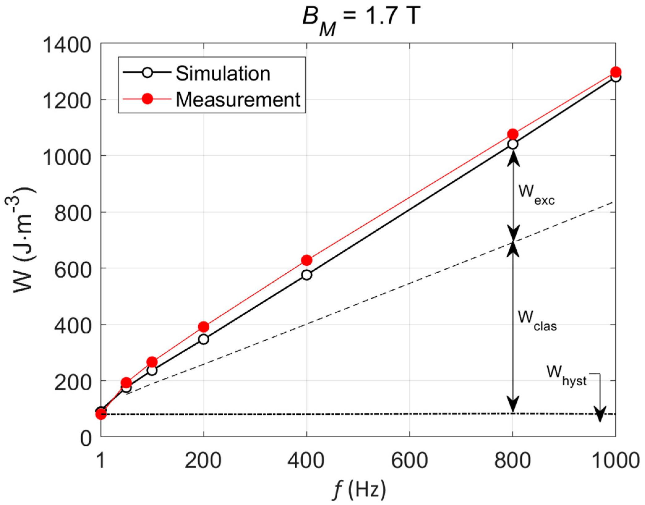
The frequency dependence of GO FeSi’s magnetic behavior, marked by phenomena such as the skin effect, defies simplistic representation through conventional modeling approaches. Despite decades of research spanning seminal contributions [9,10,11,12,13,14,15], the quest for a unified physical model capable of elucidating the dynamic B-H loop and power loss mechanisms remains elusive [16]. According to Bertotti’s statistical theory of losses (STL), the loss per magnetization cycle W at magnetizing frequency f and maximum flux density Bm can commonly be expressed as the sum of the static hysteresis loss Whyst, the classical eddy current loss Wclas, and the excess loss Wexc:
Expressions for all these terms can be found in the literature [2], such as specific experimental conditions for applying STL [17]. As mentioned in [18], STL has been used for years: “This three-term loss representation has found a wide range of applications due to its simplicity and functionality”. However, in its Bertotti form, STL is limited to the conventional frequency range, with a relatively homogeneous magnetization distribution. Also, STL can only provide losses vs. frequency predictions and not simulate any quantity in the time domain (B(t), H(t), etc.) or describe local information. This restriction is not in effect in the other classical approaches, relying on the resolution of the one-dimensional diffusion equation (where σ is the electrical conductivity [18]):
Multiple models have been developed by solving Equation (2) and a time-dependent material law. In [19], this law took the form of a first-order differential equation and yielded satisfactory results for frequencies up to f = 1 kHz, albeit with an excessive number of parameters. Similar outcomes were later achieved in [20] with a reduced, though still substantial, parameter count.
According to [18], solving Equation (2) in the case of GO FeSi inevitably leads to inaccurate results. The origin of this discrepancy is attributed to the limited proportion of classical eddy currents in the total loss. Better results over a broad frequency bandwidth are obtained in [18,21] using the so-called thin sheet model (TSM). TSM is derived from STL, expressed in its magnetic field separation form [21]:
Here, the instantaneous magnetic field strength tangent to the lamination surface is separated into hysteresis, eddy current, and excess fields. Equation (4) is the TSM fundamental equation:
Hhyst(B), also called Hstat(B) later in this paper, is a static contribution obtained from a static hysteresis model (Jiles-Atherton (J-A) model [22], Preisach model [23,24], etc.) in their B-input form. kclas is a constant depending on the specimen conductivity and geometry, δ is a directional parameter (±1), and gexc(B) and αexc(B) are two B-dependent functions that have to be defined for each frequency tested. The comparison simulations/measurements available in [18,21] reveal an excellent behavior of the TSM. Still, the number of parameters to be adjusted for each frequency level (>10 in [21]) is overwhelming, and the predictive capability of TSM is minimal. Eventually, just like STL, TSM does not provide local information.
Recent advancements in fractional calculus present novel avenues for overcoming traditional limitations [25,26], offering precise simulations across considerable frequency bandwidths while providing detailed insights into the local evolution of magnetic quantities. Our study builds upon these advancements, proposing a methodology that combines fractional derivatives with established modeling frameworks to accurately predict loss contributions across diverse frequency regimes. More precisely, this manuscript presents a comprehensive model that encapsulates the nuanced interplay between fractional calculus and magnetic losses. We outline our methodology, experimental setup, validation procedures, and critical findings, underscoring the novelty and significance of our research in advancing the understanding and predictive capabilities of soft magnetic materials.
2. Simulation Method Description
The simulation technique described in this manuscript is built based on the method initially introduced in [27], which consists of resolving simultaneously the diffusion equation (Equation (2)) and a hysteretic dynamic material law.
The specific dimensions of the tested specimens (ζ << width and length) allow us to solve the diffusion equation in one dimension (1D) using finite differences while conserving accurate results. For the material law, the simplest way would be a quasi-static hysteresis model Hstat(B). Still, it will ineluctably lead to inaccurate results as the excess loss contribution will not be considered. In [27], a first-order differential equation equivalent to a viscous behavior was proposed to improve the accuracy of the material law (Equation (5)):
Like this, the local flux density Bi became frequency dependent, and ρ was the unique parameter accounting for this effect. Still, this dependency was inaccurate, and the domain of validity of the resulting method was restrained to a narrow frequency bandwidth. Later in [19], an improvement in the frequency bandwidth was proposed, but at the cost of B-dependent additional parameters. Equation (6) was first introduced as a generalized equation in which g(B) was one of these parameters:
Then, Equation (7) was proposed in the specific case of ζ = 0.5 mm FeSi (2%) steel [16]:
Here, α(B) and β(B) were the B-dependent parameters. Unfortunately, in [16], nothing was proposed for adapting these parameters to new materials. Using multiple B-dependent parameters leads to excellent simulation results, as the method turns out to be close to a fitting process. Still, very accurate experimental data are required for implementation. The model’s predictive ability is minimal, such as the simulation setting transposability. This model was discarded for the specific case of GO FeSi [18] a few years later by the same group and replaced with the TSM.
The solution we propose to use is different and consists of a fractional derivative version of the differential Equation (5):
2.1. Fractional Differential Equation: Physical Interpretation and Resolution
Fractional calculus was first mentioned at the end of the seventeenth century [28]. Compared to classical derivatives, fractional derivative operators balance the dynamic effect distinctly. They provide the simulation method with additional freedom, resulting in precise simulations across broad frequency ranges. Fractional derivatives are intrinsically nonlocal, i.e., where classical time derivatives can only describe changes in the neighborhood of current time t, fractional ones can represent changes in a whole simulated time interval. Time fractional derivatives are recommended for long-time heavy tail decays involving the entire history. They suit ferromagnetic hysteresis, where real time behavior is significantly history dependent. In [27], Equation (5) is introduced to simulate suitably magnetic materials characterized by a homogeneous distribution of the domain wall motions and associated microscopic eddy currents. However, the diffusion related to these motions is not considered, and the domain wall motions are simulated as viscous elements. Viscoelasticity is achieved by replacing Equation (5) with Equation (8), meaning that magnetization is no longer solely dissipative but elastic, too. In mechanics, viscoelastic models employ combinations of springs and dashpots arranged in series and/or parallel [29]. Springs depict the response of an elastic solid, where stress is proportional to strain (0th-order derivative term). Dashpots represent the response of a viscous fluid, where stress is proportional to the strain rate (1st-order derivative). Using a fractional derivative of order α, where 0 < α < 1, to model a viscoelastic behavior is grounded in the notion that the actual response lies between that of a 0th and 1st-order derivative, somewhere between an elastic solid and a viscous fluid [29]. The forward Grünwald–Letnikov expression for fractional derivative respects the causality principle [25,30,31]. Therefore, it was used in this study:
Here, (n)m is the Pochhammer symbol and Γ the gamma function [29].
2.2. Combining Equation (8) and Equation (2) for a Simultaneous Resolution
In [15], we solved the loss problem by introducing the original concept of anomalous diffusion. In Equation (2), the time derivative term dB/dt was replaced by a fractional one, dnB/dtn, and σ by σ’, equivalent to a pseudo conductivity:
Simultaneous resolution of Equations (8) and (10) was possible through the concatenation in a unique expression (Equation (11)), similar to Equation (5) in [27] and constituted of H terms exclusively:
Finite differences were used to solve Equation (11), leading to a matrix system, including a stiff matrix, possibly set in post-processing. The model outputs were the average and local magnetic quantities (Hi(t), Bi(t), and B(t)). This simulation method was straightforward, and the simulation times were limited; a correct combination of ρ’ and σ’ yielded accurate results on a broad frequency bandwidth. Still, the physical meaning of the anomalous diffusion and σ’ the pseudo conductivity was unclear. The only way to derive Equation (10) was through fractional Maxwell equations. Such equations have already been mentioned in the scientific literature [32,33] but remain complex to justify physically. Therefore, this solution was discarded in this new study.
Just as Equations (8) and (10) were concatenated in [15], Equations (2) and (8) can be reformulated the same way; for this, dB/dt in Equation (8) has to be isolated:
This concatenation leads to Equation (13):
Here, again, finite differences can be applied to the left part of Equation (13) and Grünwald–Letnikov’s definition to the right part. The resulting Equation (14) is exclusively constituted of terms equivalent to magnetic fields H:
Since H(x,t) and B(x,t) are symmetric about the plane x = ζ/2, a resolution of Equation (13) on the segment [0, ζ/2] is enough, and a Neumann condition can be applied for the x = ζ/2 node (see Figure 1 for illustration). In this condition, r, the space discretization in Equation (14), is worth ζ/[2(N − 1)], where N is the number of nodes.
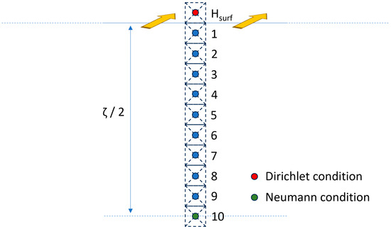
Figure 1.
1D space discretization resolution scheme, including the boundary conditions.
Equation (14) can be rewritten as below to be solved as a matrix system (Equation (15)):
where:
And [A] is the stiffness matrix:
Similar to [15], matrix [A] can be calculated in pre-processing and conserved throughout the simulation. In contrast, the matrix system has to be solved for each simulation step; it gives the local excitation field Hi(t) and is followed by a local resolution of Equation (8), leading to the local Bi(t). In the last stage, the cross-section flux density B is calculated by averaging the local induction:
Plotted as a function of the surface field Hsurf(B), the resulting simulated hysteresis cycle can be compared to the experimental one. To limit both the discretization and the memory management, such as saving simulation time, we opted for a static contribution Hstat(B) obtained with the derivative static hysteresis model (DSHM), described in [34,35]. This simulation method relies on a 2D interpolation matrix constructed with the columns and rows denoting the discrete values of H and B, and whose terms stand for the dB/dH slope at the corresponding point. As recalled in [34], DSHM can easily switch from H to B-imposed input conditions. To fill the DSHM matrix, experimental first-order reversal curves are promoted, but getting such experimental data is always complex. In this work, we replaced them with simulated first-order reversal curves obtained with the J–A model [36,37]. The J–A model was identified using the limited experimental data available (a saturated and symmetrical quasi-static hysteresis cycle). Additional details about the J–A and the DSHM models can be found elsewhere [34,35,36,37]. The next section describes the experimental setup.
3. Experimental Setup Description
Experimental works were conducted on standard Epstein-size laminations (30 mm × 305 mm) of CGO 3% SiFe, commercialized as M105-30P. The specimens have a thickness of 0.3 mm and a measured electrical conductivity of . The grains’ size (2 to 5 mm) and homogeneity are conventional for GO FeSi [38]. Electrical steel samples were magnetized using a standard double yoke single strip tester (SST) under controlled sinusoidal induction for a frequency range from 50 Hz to 1 kHz and peak flux densities of 1.0 T to 1.7 T. This measuring system complies with the British standard BS EN 10280:2007 [39]. In depth uncertainty analysis for this measuring system was performed in line with the recommendations given in UKAS M3003 [40]. Type A and B uncertainties were estimated at ± 0.30% and 0.63%, respectively. Magnetic characteristics of the steel laminations, including dynamic hysteresis loop (DHL) and bulk power loss in W·kg−1, were measured and recorded for the range of magnetizing frequency and peak induction. More details about the experimental setup are available in [41]. The following section outlines the model validation process, involving comparisons between simulations and measurements, as well as the developed method for assessing the loss contribution and distribution.
4. Simulation Method Settings and Validation up to 1 kHz and 1.7 T
The simulation method described in detail in Section 2 works with seven parameters. Five are associated with the quasi-static behavior (Hstat(B): DSHM + J–A models), while the other two are for the frequency-dependent contribution. The quasi-static contribution parameters Ms = 1.36 × 10⁶ A·m−1, a = 1.5 A·m−1, k = 11.5 A·m−1, c = 0.06, and α = 7 × 10⁻⁶ were determined based on the optimization of the relative Euclidean difference criteria (red(%), Equation (18)) comparing measured and simulated quasi-static saturated hysteresis loops (f = 1 Hz, Bm = 1.7 T).
The frequency-dependent parameters were obtained in the same way, but the experimental reference was measured at f = 1 kHz. The quasi-static contribution parameters were kept identical to the previous case at 1 Hz, and the red (%) optimization process was run to determine the two last parameters. n was obtained equal to 0.98 and ρ’ to 0.0065. Figure 2 depicts the resulting comparisons simulations/measurements in quasi-static (f = 1 Hz, Figure 2a) and f = 1 kHz (Figure 2b) conditions. N was set to 10, representing the minimum value of N that yields unvarying simulation results.
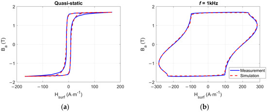
Figure 2.
(a) Comparisons simulation/measurement for f = 1 Hz, Bm = 1.7 T, (b) comparisons simulation/measurement for f = 1 kHz, Bm = 1.7 T.
4.1. Comparisons Simulation/Measurement, Model Validation
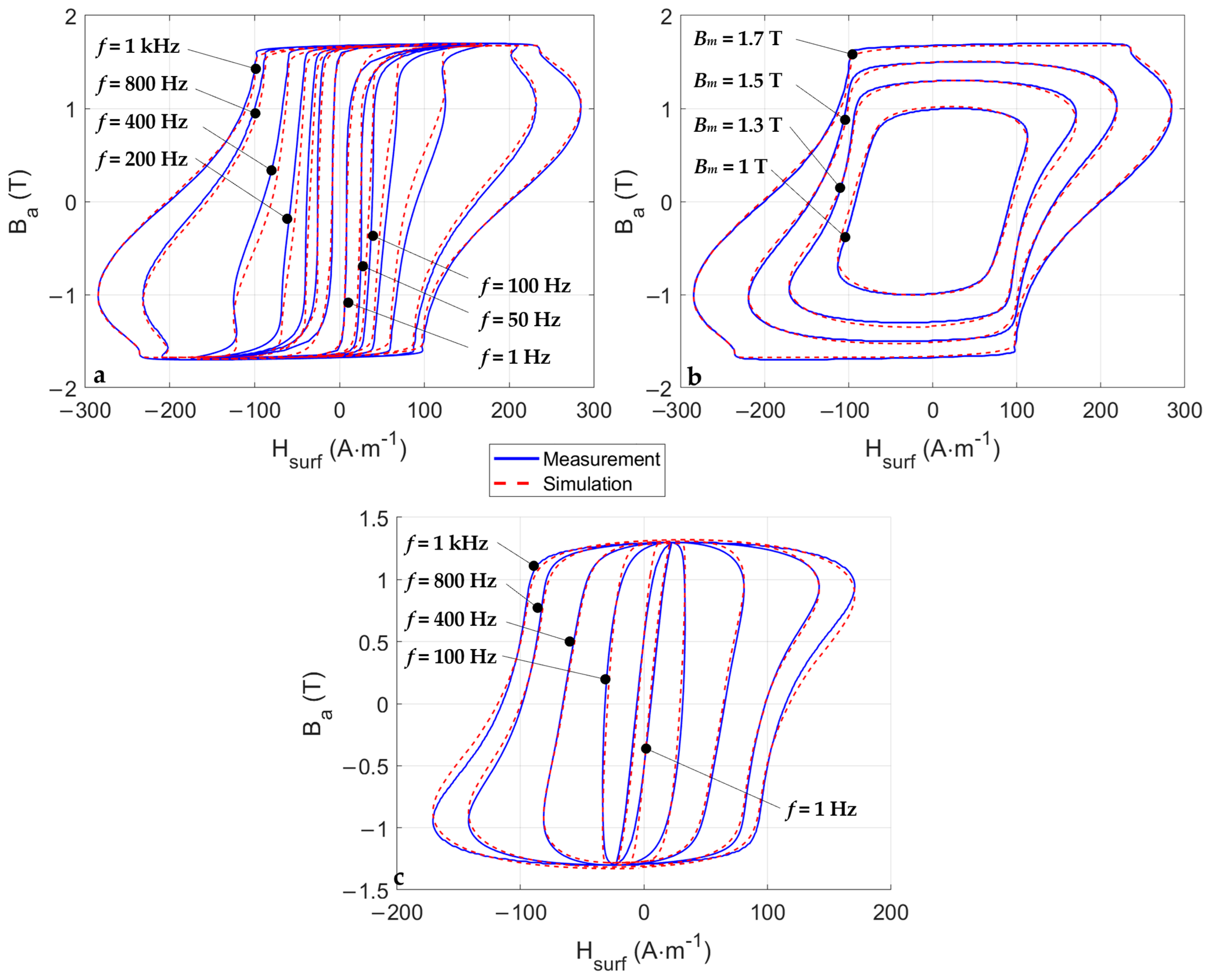
This subsection is dedicated to the validation of the simulation method; a comparison between the simulation and measurement is depicted in Figure 3. Experimental measurements were undertaken under controlled sinusoidal magnetization for the frequency range of 50 Hz to 1 kHz and peak flux density from 1.0 T to 1.7 T. This range was determined based on the magnetic flux density at which the material can potentially operate when converting electrical energy to mechanical energy, or vice versa, in typical electromagnetic devices such as transformers, electric motors, and generators [7].
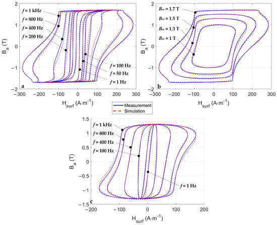
Figure 3.
(a) Comparisons simulation/measurement for f Є [1–1000] Hz, Bm = 1.7 T, (b) comparisons simulation/measurement for f = 1000 Hz, Bm Є [1–1.7] T, (c) comparisons simulation/measurement for f Є [1–1000] Hz, Bm = 1.3 T.
The accuracy and conformity of the simulation results in Figure 3 were calculated based on the red(%) and form factor (FF(%)) criteria (Equation (19) [42]), which has to be lower than 0.5 to be valid; the results are shown in Table 1.

Table 1.
Quantitative comparison (uncertainty) based on the red(%) and the FF(%) criterion for all Figure 3 simulation results (in black, the red is calculated for all contributions; in red, just the dynamic contribution) (Top table: Bm = 1.7 T; bottom table: f = 1 kHz).
As observed in the first column of Table 1, the error of the J–A model is significant (red(%) ≈ 13%) and reduces the overall accuracy of higher frequency simulations. Therefore, to have a better view of the accuracy of the dynamic contribution only, Equations (20) and (21) resolution has been applied to f Є [50–1000] Hz simulations; this led to Table 1 red results:
This method is not exact, as the space distribution of the loss contributions will change as a function of the frequency and eventually modify those percentages (this observation is especially true in the very high-frequency range). Still, it estimates the dynamic contribution accuracy closely, which in the case of the GO FeSi reaches, on average (Equation (22)), a remarkable 4.8%:
4.2. Model Exploitation, Spatial Losses Distribution
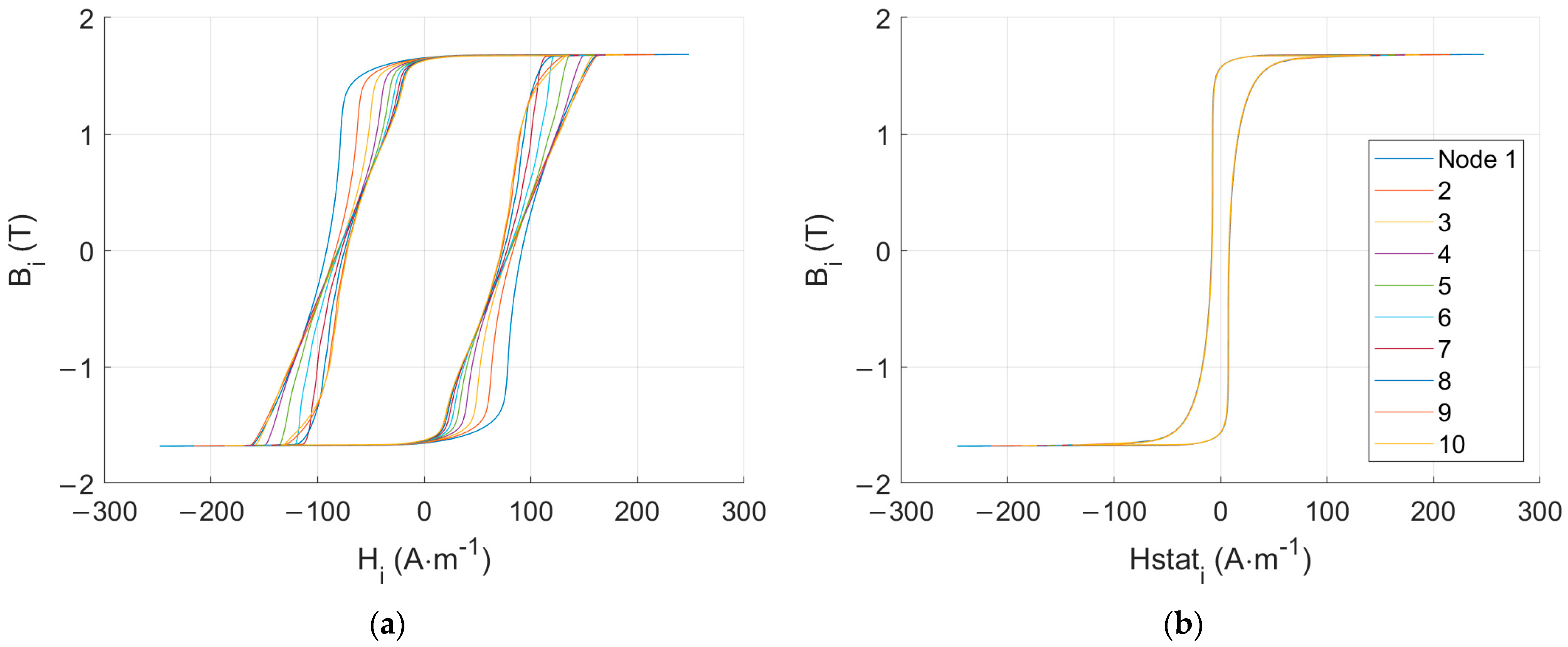
The simulation method described in this manuscript relies on the combination of the diffusion equation (Equation (2)) and a viscoelastic frequency-dependent material law (Equation (8)). An excellent property of this method comes from the space discretization associated with the finite difference resolution of Equation (2), giving access to local information. Together with the fractional differential equation material law, they lead to local static Bi(Hi stat) and dynamic Bi(Hi) hysteresis cycles. Figure 4 shows those cycles for nodes 1–10 in the case of Figure 2b, where f = 1 kHz and Bm = 1.7 T.
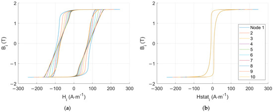
Figure 4.
(a) Local dynamic hysteresis loops (f = 1000 Hz, Bm = 1.7 T), (b) local static hysteresis loops (f = 1 Hz, Bm = 1.7 T).
Those cycles are rich in information; their areas can be associated with local energy losses. The static loops can be used to return the local hysteresis loss (Equation (23)). This contribution is frequency-independent. Then, the dynamic loops are used to return the excess loss (Equation (24)), corresponding to the additional loss associated with the frequency dependency of the domain wall motions.
The computation of the local classic loss contribution is less straightforward and needs to undergo successive steps. It starts with the calculation of the total loss:
The next step consists of the computation of the local hysteresis Whysti (Equation (23)) and excess losses Wexci (Equation (24)). Then, starting from node 1, the local classic losses Wclasi are calculated from the difference between Wtot and a virtual Wtot N=2–10 that would consider only nodes 2 to 10 for the average induction and H1 for the excitation field. The difference between Wtot and Wtot N=2–10 corresponds to Wtot1, the total loss at node 1; Wclas1 is obtained by subtracting Whyst1 and Wexc1:
This whole process is repeated in an incremental way up to node 10. Figure 5 gives the three loss contribution spatial distribution for f Є [50–1000] Hz. In this frequency range, the hysteresis loss is homogeneously distributed; both the classic and the excess loss contribution increase drastically with the frequency. Figure 6 shows the loss contributions averaged through the specimen thickness vs. frequency and the comparison with the experimental results. The large proportion of the classic loss contribution is worth noting, even if the amount of the excess loss in the total loss increases with frequency. As observed in Figure 5, the excess loss is relatively homogeneously distributed in space, unlike the classic loss, which decreases quasi-linearly. Figure 5 spatial loss distributions are impossible to confirm experimentally. The two-frequency loss separation technique is limited to the hysteresis losses (f − dependent losses) and the eddy current losses (f2 − dependent losses); this method does not provide any local information, nor can it be used to discriminate the classic and the excess losses. It was therefore discarded from the validation process.
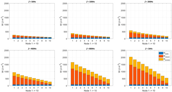
Figure 5.
Spatial loss distribution for f Є [50–1000] Hz and Bm = 1.7 T.
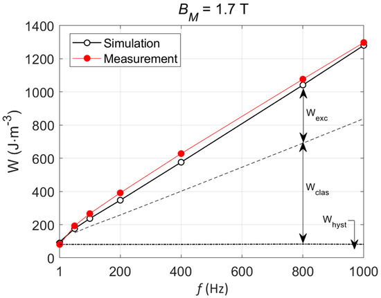
Figure 6.
Loss contributions vs. f, comparison with the experimental results.
Similarly, a computational method based on commonly known formulas such as STL could have been used as a validation method but was discarded due to its restricted frequency range of validity (f < 200 Hz, [2]).
5. Model Predictions
This section aims to leverage the predictive capability of the proposed simulation method and provide insights into the behavior at very high frequencies, where improvements in power density are anticipated. No experimental results will be provided to validate the simulation predictions. Under such operating conditions (f > 1 kHz), our experimental setup cannot yield reliable results while adhering to the standard characterization conditions.
5.1. Sinus B-Imposed Simulation
The characterization standards must be followed to obtain reproducible and comparable measurements and simulations. The characterization standards for ferromagnetic hysteresis measurement require working under sinusoidal induction. The simulation method described in this manuscript gives the magnetic response of a ferromagnetic lamination as a function of the excitation field. Simulation results shown in Figure 2 and Figure 3 were obtained by driving the model with the excitation waveforms monitored during the experimental campaign. Still, for the predictive simulations, the model has to be inversed to match the standard testing conditions. The nonhomogeneous space distribution of the flux density makes direct inversion impossible. One solution is proposed in [25] and consists of testing, for each step time, a window of field (+/− 3 A·m−1) centered around the value of H at t = t − dt. The H value that leads to the targeted B is conserved and becomes H(t). Then, the process is rerun for the next H(t + x.dt). This method only converges for minimal discretization steps, increasing the simulation time inevitably.
Therefore, in this study, we opted for an alternative and faster solution consisting of an iterative method similar to the ones used for waveform control in magnetic measurement systems. More precisely, we used the proportional−iterative learning control (P−ILC) method described in [42]. P−ILC is derived from the classical real-time proportional integral derivative (PID) technique:
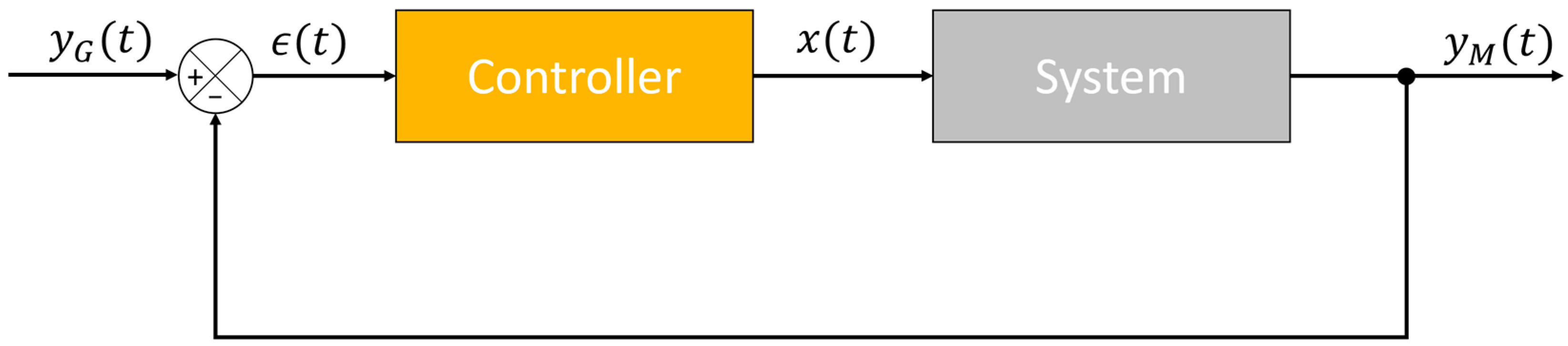
Figure 7 gives the PID feedback structure, where yM(t) is the measured output (at time t), (t) = yG(t) − yM(t) is the error, and x(t) is the system input. Kp, KI, and KD are the proportional, integral, and derivative gains, respectively.
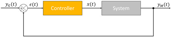
Figure 7.
Feedback structure.
The iterative PID method has been described by several authors [43] and consists of the following:
In its simplest form (proportional correction only), Equation (29) can be simplified and leads to the P−ILC formulation:
As commented in [42], P−ILC is simple; the inputs are reduced to (t,j) and the parameters to Kp. Its implementation is very straightforward, and, like classic PID, it can be very robust with the right choice of Kp.
5.2. From 2 to 10 kHz Predictions
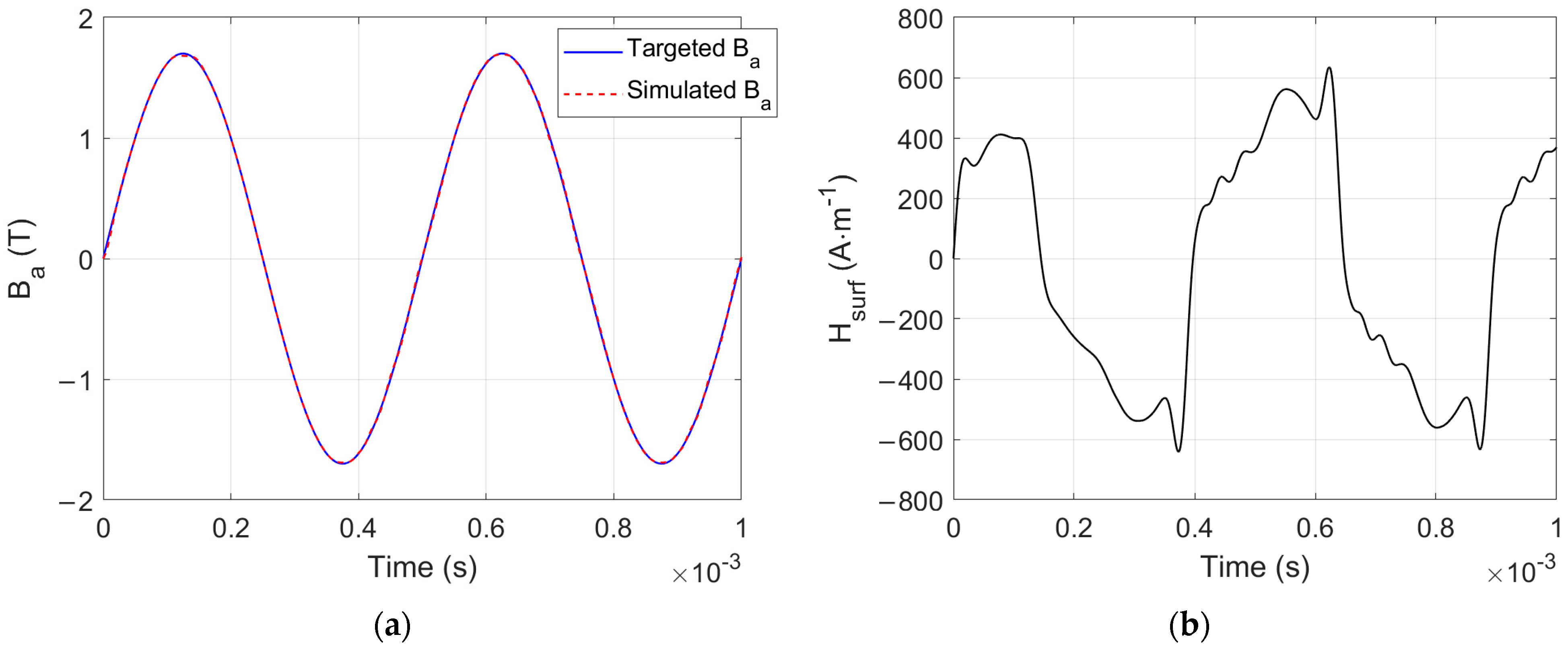
The significant temperature increase associated with the magnetization loss makes it highly complex to characterize the GO FeSi magnetic laminations beyond f = 1 kHz; such a limitation does not exist in the simulation nor in electrical machines where cooling systems are present. In the results displayed below, a low-pass filter stage was added between the controller and the system for smoother signals. P−ILC was stopped when the red(%) comparing the simulated and the targeted B reached a 1% threshold. Figure 8a illustrates the resulting comparison between the targeted flux density waveform and the simulated one at f = 1 kHz. Figure 8b shows the corresponding H.
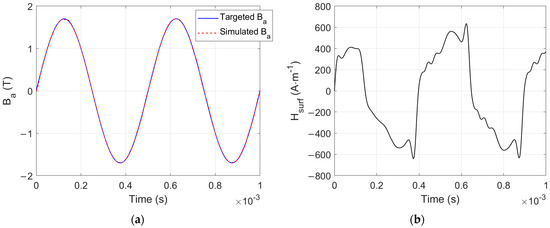
Figure 8.
(a) Comparison between the targeted and the simulated flux density at the end of the P−ILC process (f = 2 kHz), (b) H(t) related surface field.
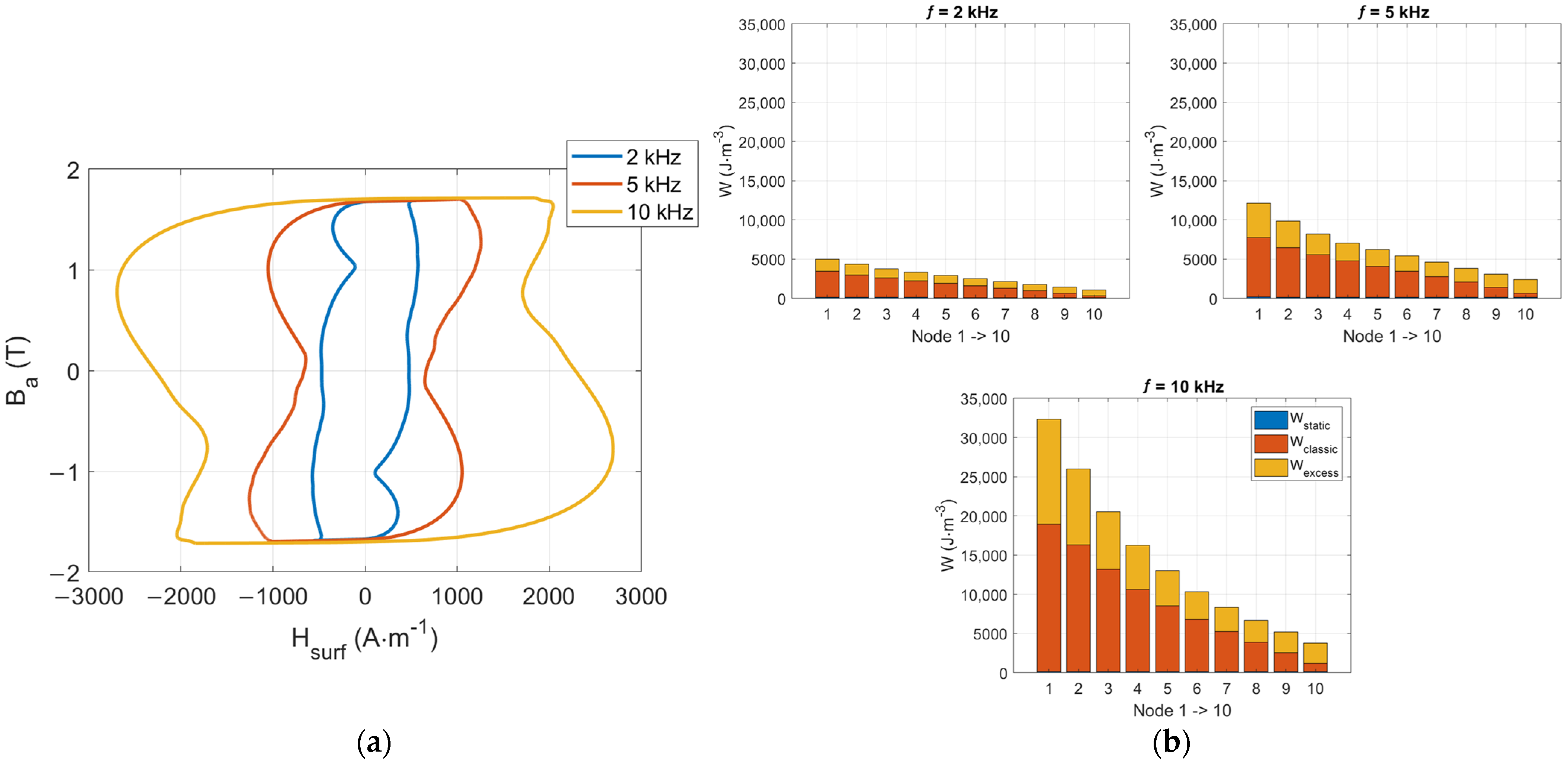
Figure 9a,b shows the 2, 5, and 10 kHz Ba(Hsurf) predictions and the associated losses in space distributions.

Figure 9.
(a) f = 2, 5 and 10 kHz, Bm = 1.7 T, B(H) simulation predictions, (b) Spatial loss distribution for f Є [2–10] kHz.
Just as expected, the level of losses increases significantly with the frequency. In the very high-frequency range, the static contribution can be considered insignificant (less than 0.6% of the total loss at f = 10 kHz). It could possibly be replaced with an anhysteretic curve in the simulation process. Figure 10 shows the extension of Figure 6 in the high-frequency range; the evolution of the excess loss proportion is worth noting.
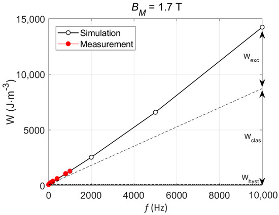
Figure 10.
Loss contributions vs. f, extension to the high-frequency range.
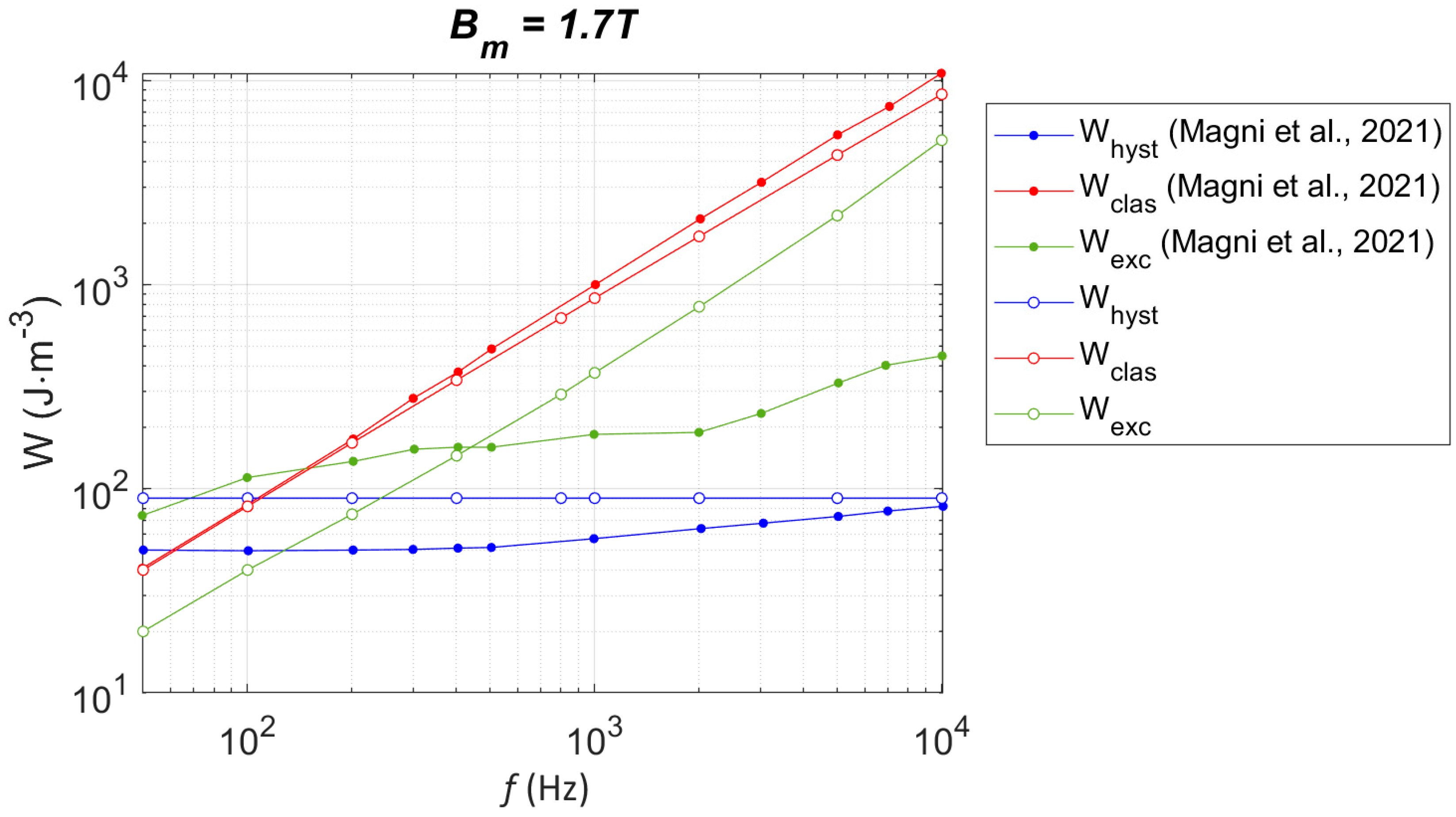
Finding experimental results beyond 1 kHz in the scientific literature is challenging. Still, in [44], authors collected experimental results at Bm = 1.7 T, f = 10 kHz on a 0.29 mm thick GO electrical steel (M2H) using a single sheet tester in a single-shot mode measurement to limit heat increase. No information is provided in the paper about using a cooling system, nor do we know how the imposed waveform for the single shot is predetermined. The only information provided is that the magnetomotive force (MMF) drop to the flux closing yoke was compensated. Then, they propose a method to predict the loss distribution. Figure 11 compares their predictions to ours.
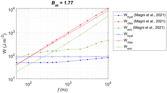
Figure 11.
Comparison of frequency-dependent loss contribution predictions between those gathered from [44] and those obtained using the method in this paper.
A relatively close behavior between Whyst and Wclass contributions is visible. The slight increase in Whyst, when f increases in [44], can be attributed to a higher level of B on the edge layers, but this behavior does not happen in our simulation method, where the static contribution illustrated in Figure 4b is always very saturated, even in a lower level of frequency. The most noticeable difference comes from the evolution of Wexc, which increases at a much lower rate in [44] than in our simulation method. The low level of Wexc in [44] is attributed to the significant skin effect in the high-frequency range (f > 200 Hz) and the absence of magnetization in the center of the tested lamination. At 1 kHz, where our simulation method has been validated through comparison with experimental results, our Wexc contribution is already three times larger than that of [44]. This difference could be attributed to the different grades of oriented grain electrical steel tested. Unfortunately, in [44], no experimental result at 1 kHz could validate this hypothesis. Finally, a slight deviation in excess loss is observable in our simulation results for the high level of f. This observation should be confirmed experimentally in future studies. Although differences can be observed in the prediction of the excess loss frequency dependency (Figure 11), the close behavior of the classic and hysteresis losses, combined with the excellent simulation results shown in Figure 2 and Figure 3, can be considered as a solid validation of our simulation method.
6. Conclusions
The problem of magnetic loss in electromagnetic converters is a classic topic. Advanced materials and new working conditions have made conventional simulation methods, such as the popular STL, obsolete. Our research introduces a novel technique involving the solution of the Maxwell diffusion equation coupled with a material law derived from a fractional differential equation. By applying this methodology, we successfully replicated the experimental B(H) hysteresis cycles of GO FeSi laminations up to f = 1 kHz, achieving a remarkable 4.8% relative Euclidean distance within the f = 50 Hz to 1 kHz bandwidth.
Several notable features distinguish our simulation method. The dynamical contribution relies on only two parameters, ρ’ (a constant) and n (the fractional order of the time-fractional derivative term). Those parameters can be set once using the f = 1 kHz experimental curve and conserved afterward. Leveraging the Grünwald−Letnikov expression for the fractional derivative enables efficient pre-calculation of the resolution coefficients and the finite difference stiffness matrix, streamlining the simulation process. The temporal resolution facilitates the simulation of diverse waveform shapes, enhancing the model’s versatility. Finally, our method offers insights into the spatial distribution of conventional loss contributions (hysteresis, classic, and excess) up to f = 10 kHz, providing valuable predictive capabilities.
Noteworthy observations and implications arise from the simulation predictions. The trajectory of loss contributions remains consistent beyond f = 1 kHz, albeit with an increasing proportion of excess loss as frequency escalates. Remarkably, even at f = 10 kHz and with Bm = 1.7 T, eddy currents resulting from the penetration equation fail to prevent magnetization of the lamination center (node 10), highlighting a significant aspect for further exploration.
This study equally opens avenues for future research and applications. Exploring the simulation method across various grades of ferromagnetic laminations promises valuable insights into magnetization mechanisms. The extension of our model to incorporate rotational magnetization behavior presents an exciting direction for further investigation [45].
In summary, this research addresses current challenges in electromagnetic converter design and lays the groundwork for future advancements in the soft ferromagnetic field.
Author Contributions
Conceptualization, B.D., P.F. and G.S.; methodology, B.D., P.F. and G.S.; validation, B.D., H.H. and Y.G.; investigation, B.D., H.H., Y.G., P.F. and G.S.; writing—original draft preparation, B.D.; writing—review and editing, H.H., Y.G., P.F. and G.S.; supervision, B.D. All authors have read and agreed to the published version of the manuscript.
Funding
This research received no external funding.
Data Availability Statement
Data are available on request due to privacy/ethical restrictions.
Conflicts of Interest
The authors declare no conflicts of interest.
References
- Silveyra, J.M.; Ferrara, E.; Huber, D.L.; Monson, T.C. Soft magnetic materials for a sustainable and electrified world. Science 2018, 362, eaao0195. [Google Scholar] [CrossRef]
- Bertotti, G. Hysteresis in Magnetism: For Physicists, Materials Scientists, and Engineers; Gulf Professional Publishing: Houston, TX, USA, 1998. [Google Scholar]
- Krings, A.; Boglietti, A.; Cavagnino, A.; Sprague, S. Soft magnetic material status and trends in electric machines. IEEE Trans. Ind. Electron. 2016, 64, 2405–2414. [Google Scholar] [CrossRef]
- Zhao, H.; Ragusa, C.; Appino, C.; de la Barrière, O.; Wang, Y.; Fiorillo, F. Energy losses in soft magnetic materials under symmetric and asymmetric induction waveforms. IEEE Trans. Power Electron. 2018, 34, 2655–2665. [Google Scholar] [CrossRef]
- Herzer, G. Modern soft magnets: Amorphous and nanocrystalline materials. Acta Mater. 2013, 61, 718–734. [Google Scholar] [CrossRef]
- Xia, Z.; Kang, Y.; Wang, Q. Developments in the production of grain-oriented electrical steel. J. Magn. Magn. Mater. 2008, 320, 3229–3233. [Google Scholar] [CrossRef]
- Fiorillo, F.; Bertotti, G.; Appino, C.; Pasquale, M. Soft magnetic materials. In Wiley Encyclopedia of Electrical and Electronics Engineering; John Wiley & Sons, Inc.: Hoboken, NJ, USA, 2011; pp. 1–42. [Google Scholar]
- Hayakawa, Y. Mechanism of secondary recrystallization of Goss grains in grain-oriented electrical steel. Sci. Technol. Adv. Mater. 2017, 18, 480–497. [Google Scholar] [CrossRef]
- Bertotti, G. Physical interpretation of eddy current losses in ferromagnetic materials. I. Theoretical considerations. J. Appl. Phys. 1985, 57, 2110–2117. [Google Scholar] [CrossRef]
- Shilyashki, G.; Pfützner, H.; Bengtsson, C.; Huber, E. Time-averaged and instantaneous magnetic loss characteristics of different products of electrical steel for frequencies of 16 2/3 Hz up to 500 Hz. IET Electr. Power Appl. 2022, 16, 525–535. [Google Scholar] [CrossRef]
- Chwastek, K.R. The effects of sheet thickness and excitation frequency on hysteresis loops of non-oriented electrical steel. Sensors 2022, 22, 7873. [Google Scholar] [CrossRef]
- Ducharne, B.; Zhang, S.; Sebald, G.; Takeda, S.; Uchimoto, T. Electrical steel dynamic behavior quantitated by inductance spectroscopy: Toward prediction of magnetic losses. J. Magn. Magn. Mater. 2022, 560, 169672. [Google Scholar] [CrossRef]
- Pfützner, H.; Shilyashki, G.; Huber, E. Calculated versus measured iron losses and instantaneous magnetization power functions of electrical steel. Electr. Eng. 2022, 104, 2449–2455. [Google Scholar] [CrossRef] [PubMed]
- He, Z.; Kim, J.S.; Koh, C.S. An Improved Model for Anomalous Loss Utilizing Loss Separation and Comparison with ANN Model in Electrical Steel Sheet. IEEE Trans. Magn. 2022, 58, 1–5. [Google Scholar] [CrossRef]
- Ducharne, B.; Sebald, G. Combining a fractional diffusion equation and a fractional viscosity-based magneto dynamic model to simulate the ferromagnetic hysteresis losses. AIP Adv. 2022, 12, 035029. [Google Scholar] [CrossRef]
- Moses, A.J. Energy efficient electrical steels: Magnetic performance prediction and optimization. Scr. Mater. 2012, 67, 560–565. [Google Scholar] [CrossRef]
- De la Barriere, O.; Ragusa, C.; Appino, C.; Fiorillo, F. Prediction of energy losses in soft magnetic materials under arbitrary induction waveforms and DC bias. IEEE Trans. Ind. Electron. 2016, 64, 2522–2529. [Google Scholar] [CrossRef]
- Zirka, S.E.; Moroz, Y.I.; Steentjes, S.; Hameyer, K.; Chwastek, K.; Zurek, S.; Harrison, R.G. Dynamic magnetization models for soft ferromagnetic materials with coarse and fine domain structures. J. Magn. Magn. Mater. 2015, 394, 229–236. [Google Scholar] [CrossRef]
- Zirka, S.E.; Moroz, Y.I.; Marketos, P.; Moses, A.J. Viscosity-based magnetodynamic model of soft magnetic materials. IEEE Trans. Magn. 2006, 42, 2121–2132. [Google Scholar] [CrossRef]
- Petrun, M.; Steentjes, S. Iron-loss and magnetization dynamics in non-oriented electrical steel: 1-D excitations up to high frequencies. IEEE Access 2020, 8, 4568–4593. [Google Scholar] [CrossRef]
- Zirka, S.E.; Moroz, Y.I.; Marketos, P.; Moses, A.J.; Jiles, D.C.; Matsuo, T. Generalization of the classical method for calculating dynamic hysteresis loops in grain-oriented electrical steels. IEEE Trans. Magn. 2008, 44, 2113–2126. [Google Scholar] [CrossRef]
- Sadowski, N.; Batistela, N.J.; Bastos, J.P.A.; Lajoie-Mazenc, M. An inverse Jiles-Atherton model to take into account hysteresis in time-stepping finite-element calculations. IEEE Trans. Magn. 2002, 38, 797–800. [Google Scholar] [CrossRef]
- Davino, D.; Giustiniani, A.; Visone, C. Fast inverse Preisach models in algorithms for static and quasi-static magnetic-field computations. IEEE Trans. Magn. 2008, 44, 862–865. [Google Scholar] [CrossRef]
- Cardelli, E.; Torre, E.D.; Tellini, B. Direct and inverse Preisach modeling of soft materials. IEEE Trans. Magn. 2000, 36, 1267–1271. [Google Scholar] [CrossRef]
- Ducharne, B.; Sebald, G. Fractional derivatives for the core losses prediction: State of the art and beyond. J. Magn. Magn. Mater. 2022, 563, 169961. [Google Scholar] [CrossRef]
- Liu, R.; Li, L. Analytical prediction model of energy losses in soft magnetic materials over broadband frequency range. IEEE Trans. Power Electron. 2020, 36, 2009–2017. [Google Scholar] [CrossRef]
- Raulet, M.A.; Ducharne, B.; Masson, J.P.; Bayada, G. The magnetic field diffusion equation including dynamic hysteresis: A linear formulation of the problem. IEEE Trans. Magn. 2004, 40, 872–875. [Google Scholar] [CrossRef]
- Samko, S.G. Fractional integrals and derivatives. In Theory Applications; Springer: Berlin/Heidelberg, Germany, 1993. [Google Scholar]
- Meral, F.C.; Royston, T.J.; Magin, R. Fractional calculus in viscoelasticity: An experimental study. Commun. Nonlinear Sci. Numer. Simul. 2010, 15, 939–945. [Google Scholar] [CrossRef]
- Ortigueira, M.; Machado, J. Which derivative? Fractal Fract. 2017, 1, 3. [Google Scholar] [CrossRef]
- Ortigueira, M.; Machado, J. Fractional definite integral. Fractal Fract. 2017, 1, 2. [Google Scholar] [CrossRef]
- Tarasov, V.E. Fractional vector calculus and fractional Maxwell’s equations. Ann. Phys. 2008, 323, 2756–2778. [Google Scholar] [CrossRef]
- Ortigueira, M.D.; Rivero, M.; Trujillo, J.J. From a generalised Helmholtz decomposition theorem to fractional Maxwell equations. Commun. Nonlinear Sci. Numer. Simul. 2015, 22, 1036–1049. [Google Scholar] [CrossRef]
- Scorretti, R.; Sabariego, R.V.; Sixdenier, F.; Ducharne, B.; Raulet, M.A. Integration of a New Hysteresis Model in the Finite Elements Method. Compumag 2011. 2011, p. n-334. Available online: https://hal.science/hal-00582555/ (accessed on 8 December 2023).
- Fagan, P.; Ducharne, B.; Skarlatos, A. Optimized magnetic hysteresis management in numerical electromagnetic field simulations. In Proceedings of the 2021 IEEE International Magnetic Conference (INTERMAG), Lyon, France, 26–30 April 2021; pp. 1–5. [Google Scholar]
- Jiles, D.C.; Atherton, D.L. Theory of ferromagnetic hysteresis. J. Magn. Magn. Mater. 1986, 61, 48–60. [Google Scholar] [CrossRef]
- Jiles, D. Introduction to Magnetism and Magnetic Materials; CRC Press: Boca Raton, FL, USA, 2015. [Google Scholar]
- Chen, N.; Zaefferer, S.; Lahn, L.; Günther, K.; Raabe, D. Effects of topology on abnormal grain growth in silicon steel. Acta Mater. 2003, 51, 1755–1765. [Google Scholar] [CrossRef]
- BS EN 10280:2001 + A1:2007; Magnetic Materials-Methods of Measurement of the Magnetic Properties of Electrical Sheet and Strip by Means of a Single Sheet Tester. BSI: Alameda, CA, USA, 2001.
- UKAS. M3003-The Expression of Uncertainty and Confidence in Measurement, 4th ed.; United Kingdom Accreditation Service: Staines, UK, 2019. [Google Scholar]
- Hamzehbahmani, H.; Anderson, P.; Jenkins, K. Interlaminar insulation faults detection and quality assessment of magnetic cores using flux injection probe. IEEE Trans. Power Deliv. 2015, 30, 2205–2214. [Google Scholar] [CrossRef]
- Fagan, P.; Ducharne, B.; Zurek, S.; Domenjoud, M.; Skarlatos, A.; Daniel, L.; Reboud, C. Iterative methods for waveform control in magnetic measurement systems. IEEE Trans. Instrum. Meas. 2022, 71, 1–13. [Google Scholar] [CrossRef]
- Gruebler, H.; Krall, F.; Leitner, S.; Muetze, A. Loss-surface-based iron loss prediction for fractional horsepower electric motor design. In Proceedings of the 2018 20th European Conference on Power Electronics and Applications (EPE’18 ECCE Europe), Riga, Latvia, 17–21 September 2018; p. P-1. [Google Scholar]
- Magni, A.; Sola, A.; de La Barriere, O.; Ferrara, E.; Martino, L.; Ragusa, C.; Appino, C.; Fiorillo, F. Domain structure and energy losses up to 10 kHz in grain-oriented Fe-Si sheets. AIP Adv. 2021, 11, 015220. [Google Scholar] [CrossRef]
- Ducharne, B.; Zurek, S.; Sebald, G. A universal method based on fractional derivatives for modeling magnetic losses under alternating and rotational magnetization conditions. J. Magn. Magn. Mater. 2022, 550, 169071. [Google Scholar] [CrossRef]


Disclaimer/Publisher’s Note: The statements, opinions and data contained in all publications are solely those of the individual author(s) and contributor(s) and not of MDPI and/or the editor(s). MDPI and/or the editor(s) disclaim responsibility for any injury to people or property resulting from any ideas, methods, instructions or products referred to in the content. |
© 2024 by the authors. Licensee MDPI, Basel, Switzerland. This article is an open access article distributed under the terms and conditions of the Creative Commons Attribution (CC BY) license (https://creativecommons.org/licenses/by/4.0/).