Abstract
This paper is dedicated to optimizing the functionality of Microgrid-Integrated Charging Stations (MICCS) through the implementation of a new control strategy, specifically the fractional-order proportional-integral (FPI) controller, aided by a hybrid optimization algorithm. The primary goal is to elevate the efficiency and stability of the MICCS-integrated inverter, ensuring its seamless integration into modern energy ecosystems. The MICCS system considered here comprises a PV array as the primary electrical power source, complemented by a proton exchange membrane fuel cell as a supporting power resource. Additionally, it includes a battery system and an electric vehicle charging station. The optimization model is formulated with the objective of minimizing the integral of square errors in both the DC-link voltage and grid current while also reducing total harmonic distortion. To enhance the precision of control parameter estimation, a hybrid of the one-to-one optimizer and sine cosine algorithm (HOOBSCA) is introduced. This hybrid approach improves the exploitation and exploration characteristics of individual algorithms. Different meta-heuristic algorithms are tested against HOOBSCA in different case studies to see how well it tunes FPI settings. Findings demonstrate that the suggested method improves the integrated inverters’ transient and steady-state performance, confirming its improved performance in generating high-quality solutions. The best fitness value achieved by the proposed optimizer was 3.9109, outperforming the other algorithms investigated in this paper. The HOOBSCA-based FPI successfully improved the response of the DC-link voltage, with a maximum overshooting not exceeding 8.5% compared to the other algorithms employed in this study.
1. Introduction
In recent years, the integration of electric vehicles (EVs) into our transportation infrastructure has surged, driven by the global pursuit of sustainable and eco-friendly mobility solutions. Microgrids (MGs) have arisen as a leading approach to tackle the issues brought about by the extensive use of EVs, and this paradigm shift calls for the creation of sophisticated energy management systems [1,2]. A microgrid, characterized by its localized and decentralized energy generation and distribution capabilities, offers a promising framework for the seamless integration of EV charging stations. This integration holds immense potential to not only enhance the reliability and efficiency of electric vehicle charging but also to contribute to the overall resilience and sustainability of the broader energy ecosystem. This introductory exploration delves into the synergistic relationship between MGs and EV charging stations, shedding light on the transformative impact they can collectively exert on the landscape of modern transportation and energy infrastructure [3,4].
MGs are versatile and dynamic energy systems that come in various types, each tailored to meet specific needs and circumstances. One prevalent classification is based on their interconnection to the main power grid: grid-tied, off-grid, and hybrid microgrids. Grid-tied microgrids are seamlessly integrated with the main electrical grid, allowing for a bidirectional flow of electricity [5,6,7]. In times of peak demand, these MGs can pull power from the grid, and in times of surplus, they can feed back the extra energy they have generated. In contrast, microgrids that are off grid operate entirely on renewable energy sources and battery storage without connecting to the main power grid. A versatile and dependable energy solution, hybrid MGs integrate grid-tied and off-grid components to balance renewable power sources’ variable output with conventional grid access. Furthermore, MGs can be classified according to their main use, with different types servicing different geographic or functional regions. For example, there are remote microgrids, campus microgrids, and community microgrids. The versatility and importance of microgrids in attaining energy resilience and sustainability are highlighted by their vast range of kinds.
Direct Current (DC)- and Alternating Current (AC)-based MGs represent two distinct approaches to local energy distribution with unique characteristics and applications [8]. DC microgrids utilize direct current for the transmission and distribution of electricity. DC systems are particularly well-suited to be integrated with renewable energy sources, such as solar panels and batteries, as these technologies inherently generate or store DC power. DC MGs are known for their efficiency in local distribution, especially in data centers, telecommunications, and certain industrial applications. On the other hand, AC microgrids rely on the traditional AC power format. AC MGs are more prevalent and compatible with the existing grid infrastructure, making them suitable for broader applications, including residential, commercial, and industrial settings [9,10]. AC MGs offer flexibility in connecting with diverse energy sources and loads, and they can efficiently transmit electricity over longer distances. Both DC and AC MGs play vital roles in enhancing energy resilience, promoting sustainability, and addressing specific energy needs in various contexts. The choice between DC and AC MGs depends on factors such as the local energy ecosystem, the nature of energy sources, and the specific requirements of the end-users [11].
EV charging stations are critical infrastructure for the widespread adoption of electric vehicles, serving as the interface between the electrical grid and EVs. These stations can be classified into various topology structures, including Level 1, Level 2, and DC fast charging [12,13]. Level 1 chargers typically operate on standard household 120-volt outlets and provide slow charging, suitable for overnight charging at home. Level 2 chargers use 240-volt outlets and offer faster charging, and they are commonly found in residential, commercial, and public settings. DC fast-charging stations, on the other hand, supply high-voltage DC power directly to the EV’s battery, enabling rapid charging within minutes and are typically deployed along highways and in urban areas to support long-distance travel.
Recent advancements in EV charging infrastructure have revolutionized the efficiency, reliability, and convenience of charging processes [14,15]. One notable area of progress is in ultra-fast charging technologies, where research and development efforts aim to significantly reduce charging times. Innovations such as high-power charging systems, advanced battery management techniques, and effective cooling solutions are being explored to enable faster charging while maintaining battery longevity. Additionally, the emergence of wireless charging technology has garnered attention, offering EVs the ability to charge simply by parking over a charging pad embedded in the ground, eliminating the need for physical cables. Despite being in early stages of deployment, wireless charging presents a promising solution for urban environments and fleet applications, enhancing convenience and ease of use. Moreover, smart charging solutions are leveraging communication technologies and data analytics to optimize charging processes based on grid conditions, electricity prices, and user preferences. These systems enable load management, peak shaving, and demand response capabilities, ensuring efficient utilization of electricity resources while minimizing grid impacts. Battery-swapping stations have also emerged as a rapid alternative to traditional charging, allowing EVs to exchange depleted batteries for fully charged ones and addressing concerns about long charging times and range anxiety, particularly in commercial fleets. Integration with renewable energy sources such as solar and wind power further enhances the sustainability of EV charging infrastructure, reducing reliance on the grid and lowering carbon emissions. Finally, user experience enhancements, including mobile apps, digital payment systems, real-time availability updates, and personalized charging recommendations, streamline the charging experience for EV drivers, fostering greater adoption of electric vehicles [15,16].
The integration of EV charging stations in MGs necessitates a comprehensive and adaptive control strategy. Microgrid controllers must be capable of handling the dynamic nature of EV charging loads, optimizing energy management, and ensuring the overall stability and reliability of the MG in the presence of these additional and variable loads. Various controller algorithms are applied to enhance MG performance, each serving specific purposes based on the MG’s characteristics, operational requirements, and objectives [17]. Often, a combination of these controllers may be employed to address different aspects of MG operation and enhance overall performance. The Proportional-Integral-Derivative (PID) Controller is a widely used algorithm that regulates the MG’s output by adjusting the control variables proportionally to the error, its integral, and derivative over time. It is effective in stabilizing and optimizing the performance of MGs by maintaining key parameters within desired ranges. Fuzzy Logic Controllers (FLC) are also employed to manage uncertainty and non-linearity, making them particularly useful for optimizing power flow, voltage regulation, and energy storage systems. Model Predictive Control (MPC) is an advanced control strategy that utilizes a dynamic model of the MG to predict future states and optimize control inputs over a specified prediction horizon. MPC is effective in optimizing various MG objectives, such as minimizing energy costs, ensuring grid stability, and managing renewable energy sources [18,19].
The application of a Fractional Order Proportional-Integral-Derivative (FOPID) controller in MGs with EVs can significantly enhance performance by addressing specific challenges associated with dynamic and nonlinear systems. A FOPID controller is an extension of the traditional PID controller where the proportional (P), integral (I), and derivative (D) components have fractional orders [20,21,22]. In contrast to standard PID controllers, which use integer orders for these components, fractional order controllers introduce fractional exponents for the calculus operators, allowing for a more flexible and nuanced control strategy. FOPID controllers are frequently used to improve the transient response, minimizing overshoot and the settling time of MGs involving EV charging stations. The flexibility of FOPID components enhances the controller’s robustness in face of uncertainties and variations in the controlled system [23,24].
The tuning of PID or FOPID controllers has become a focal point in control engineering, given their enhanced capability to model complex dynamical systems. Various methods have been proposed to systematically tune the parameters of PID and FOPID controllers, aiming to optimize system performance. One common approach involves employing optimization algorithms to iteratively search for optimal fractional orders and gains. Another method leverages the frequency domain, utilizing Bode plots and Nyquist diagrams to analyze the system’s response and adjust controller parameters accordingly. Additionally, heuristic methods, including the Ziegler–Nichols method adapted for fractional order systems [25], have been explored. Despite the challenges posed by the non-integer nature of fractional orders, the development of efficient tuning strategies for FOPID controllers is crucial for their widespread application in diverse and intricate control scenarios.
Ali et al. [26] utilized FOPID controllers to regulate the back-to-back configuration of an Archimedes wave swing energy conversion system with the objective of maximizing wave energy yield while maintaining predetermined values for grid voltage and capacitor DC link voltage. Six FOPID controllers were employed, requiring the fine-tuning of thirty parameters. To optimize these control gains, a hybrid jellyfish search optimizer and particle swarm optimization algorithm were employed. The efficiency of the proposed FOPID control system was proven through a performance comparison with two traditional PID controllers and one FOPID controller. Ali et al. [27] suggested employing a cascaded Proportional Integral-Fractional Order Proportional-Integral-Derivative (PI-FOPID) controller to enhance the frequency response of a hybrid MG system. The optimal gains of this controller are precisely adjusted using the Gorilla Troops Optimizer (GTO). To evaluate its efficacy, the routine of the proposed cascaded PI-FOPID controller is compared with that of a single-structure FOPID controller, tuned using GTO, as well as various other optimization techniques found in previous literature, such as Genetic Algorithm (GA) and Particle Swarm Optimization (PSO). In Murugesan et al. [28], cohort intelligence optimization was utilized to fine-tune the five primary gain values of FPID regulators. The effectiveness of the proposed FOPID regulator tuned by cohort intelligence was assessed by comparing it with a conventional PID controller tuned using GA and PSO in identical single and dual control area MG systems.
In Roslan et al. [29], the PI controller parameters were fine-tuned using the PSO technique. This involved minimizing the error associated with the voltage regulator and current controller schemes within the inverter system. Hussien et al. [30] introduced an innovative approach for optimizing the control of isolated MGs through the utilization of the coot bird metaheuristic optimizer (CBMO). The primary focus is on determining the optimal gains for the PI controller within a multi-objective optimization framework using CBMO. The efficacy of the proposed optimizer is substantiated through a comparative analysis against results obtained from LMSRE-based adaptive control, the sunflower optimization algorithm, the Ziegler–Nichols method, and PSO. Ellithy et al. [31] presented a distinctive algorithmic approach using the Marine Predator Algorithm for the optimal tuning of the PI controller, specifically focusing on inverter control to enhance the Low Voltage Ride-Through capability of the grid. This improvement extends to addressing overshoot, undershoot, settling time, and steady-state response of the system. To assess its effectiveness, the proposed approach is compared to competing basic optimization-based PI controllers, namely Grey Wolf Optimization and PSO. In Dhar et al. [32], the water cycle optimization method was applied to attain optimal control of a solar photovoltaic MG with battery storage. This approach was employed to precisely adjust parameters of the PI controllers, ensuring effective regulation of both the battery current and the DC-link voltage.
In this paper, an enhanced control strategy for MG-integrated charging stations (MICCS) using a fractional-order PI controller (FPI) is proposed. To accurately estimate the controller parameters, the optimization model focuses on minimizing the integral of square error and the total harmonic distortion, thereby enhancing the overall performance. The proposed control strategy aims to expand the existing toolbox of methods available for controlling MICCS. This approach offers a promising avenue for improving the quality of control strategies in MG-integrated charging stations. The main contributions of this paper can be summarized as follows:
- A novel hybrid algorithm that combines the one-to-one-based optimizer and the sine cosine algorithm is developed to estimate the parameters of the FPI controller.
- The proposed optimization model is formulated with the aim of enhancing several aspects of performance. The fitness function is designed to optimize the DC-link voltage of the inverter, enhance the response of both the direct and quadrature axis currents, and concurrently improve power quality by reducing the total harmonic distortion in the grid current.
The subsequent sections of this paper are structured as follows: Section 2 delineates the modeling of the proposed system and outlines the optimization model. In Section 3, the hybrid one-to-one optimizer and the sine cosine algorithm proposed in this study are detailed. Section 4 presents the results and corresponding discussions, while Section 5 encapsulates the conclusion of the paper.
2. Microgrid Structure
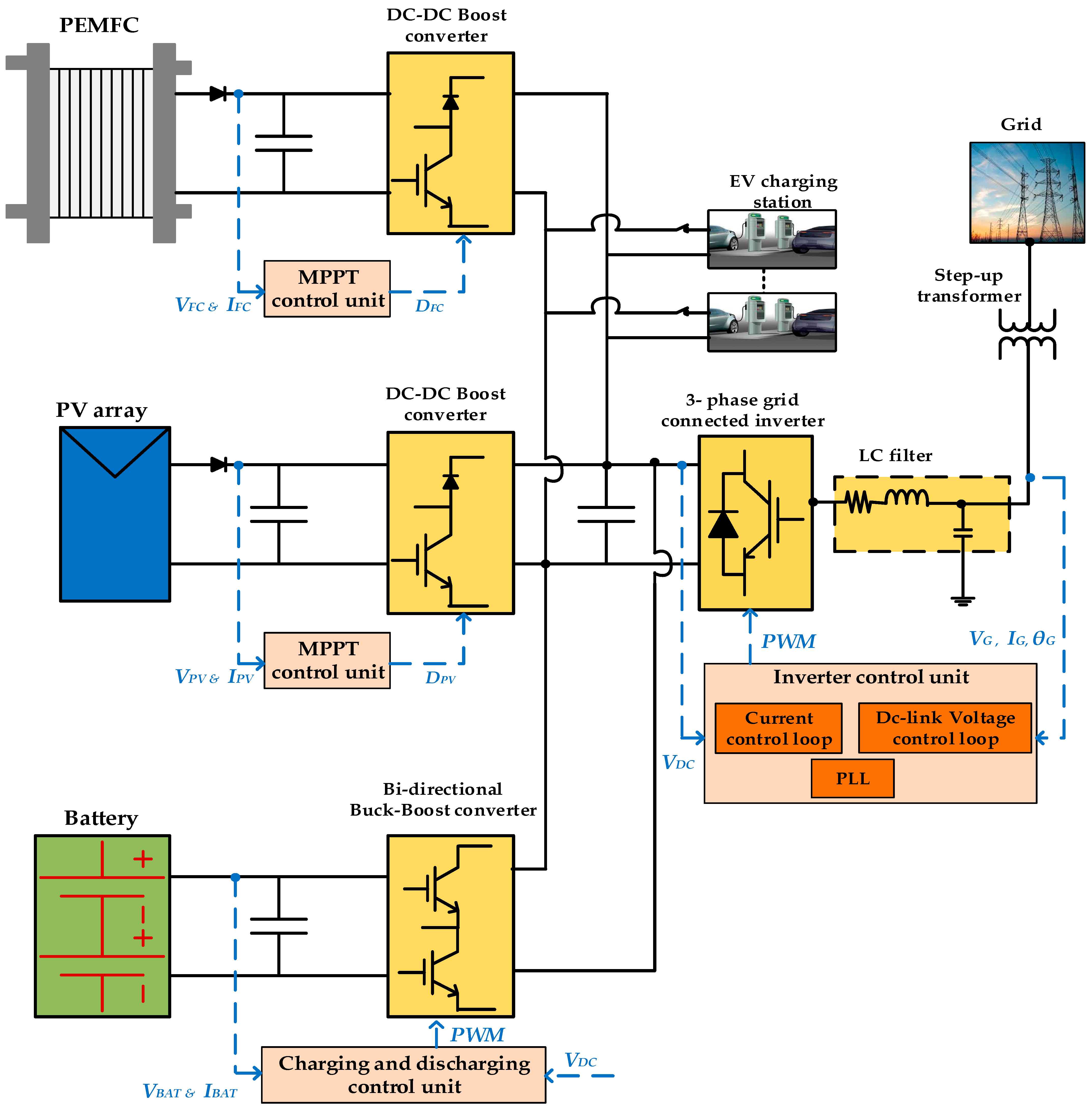
The MG system employed in this study is designed to integrate diverse RESs and energy storage technologies, creating a versatile and sustainable energy infrastructure. The key components of the MG include a fuel cell, photovoltaic (PV) array, battery system, bidirectional DC–DC converter, grid-connected inverter, and charging stations as depicted in Figure 1. Dash lines present the measured signals, while solid lines present the connection between the power devices.
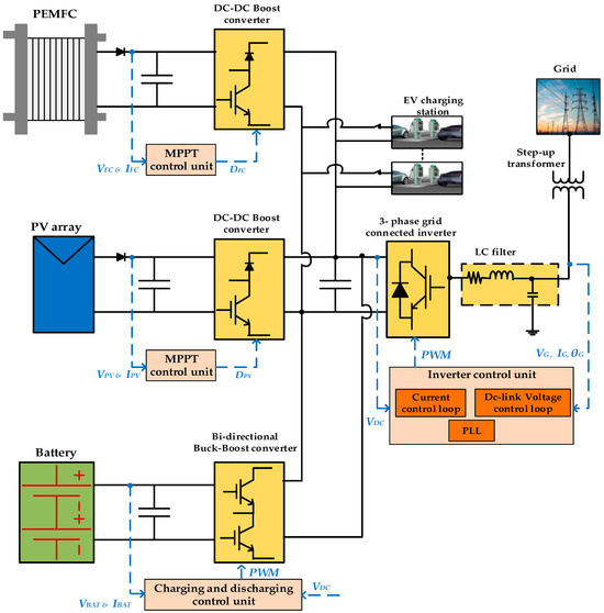
Figure 1.
Structure of the tested MG.
The MG incorporates a 100-kW photovoltaic array as a primary power generation source. The PV array consists of 66 strings, and each string comprises five modules connected in series. The module characteristics are given in Table 1. Complementing the PV array, a fuel cell system is integrated into the microgrid, contributing to the overall energy mix and reducing dependence on non-renewable sources. The fuel cell utilizes hydrogen to convert chemical energy into electrical energy, ensuring a constant and reliable power supply. The characteristics of the PEM fuel cell used in this study are presented in Table 2. A sophisticated battery system is integrated to store excess energy generated during peak production periods. This energy reservoir serves as a crucial element for balancing supply and demand, providing stability to the MG and ensuring an uninterrupted power supply. The bidirectional DC–DC converter plays a pivotal role in managing the flow of energy between different components of the MG. This converter facilitates efficient energy transfer, allowing for seamless integration of the fuel cell, PV array, and battery system.

Table 1.
Characteristics of SunPower SPR-305-WHT PV module (SunPower, California, United States of America).
To enable the MG to interact with the main chief grid, a grid-connected inverter is employed. This device converts direct current from the MG into alternating current, ensuring compatibility with the grid and enabling bidirectional power flow. The MG is equipped with charging stations designed for EVs and other electric-powered devices. These stations are strategically placed to support sustainable transportation and contribute to the overall eco-friendly objectives of the MG system.
To ensure the stable and efficient operation of the microgrid (MG) under consideration, two Maximum Power Point Tracking (MPPT) control units are devised to enhance the performance of both the Proton Exchange Membrane Fuel Cell (PEMFC) and the PV array. Additionally, a battery control unit is formulated to regulate the charging and discharging current of the battery system. Finally, a fractional-order PI controller is employed in the design of the inverter control unit. The subsequent sections introduce the mathematical model of the microgrid components under investigation. Additionally, we elaborate on the parameters and structure of the fractional-order PI controller tuning strategy. Validation of the proposed control strategy is conducted using Matlab/Simulink r2021a software.
2.1. Modelling of the PEM Fuel Cell Subsystem
One form of fuel cell is the polymer electrolyte membrane fuel cell, or PEMFC. Electrochemical fuel cells use a redox process to transform chemical energy into electrical energy. Because of its versatility and efficiency, PEM fuel cells have gained a lot of attention. The heart of a PEM fuel cell is the polymer electrolyte membrane, typically made of a special polymer material. This membrane allows positively charged ions (protons) to pass through while blocking electrons. The membrane separates the anode and cathode compartments [33,34].
At the anode (negative electrode), hydrogen gas is typically supplied. The hydrogen molecules are split into protons and electrons through a catalytic reaction. The protons generated at the anode move through the electrolyte membrane to the cathode. The electrons, however, cannot pass through the membrane. At the cathode (positive electrode), oxygen (usually from the air) is supplied. The protons arriving from the anode combine with electrons from the external circuit and oxygen to form water. The electrons, which cannot pass through the membrane, are forced to travel through an external electrical circuit, creating an electric current that can be used to power electrical devices.
Mathematically, the output voltage of the fuel cell stack containing NFC cells can be calculated using the following expression [35,36]:
Subsequently, the power generated by the PEMFC can be determined by [35,36]:
The symbol IFC represents the fuel cell current measured in Amperes (amp), while Vcell denotes the output voltage of a single cell. The calculation for Vcell is as follows [35,36]:
where Enernst is the cell electric potential, also known as the Nernst equation, calculated by Equation (4). Vact signifies the voltage reduction caused by reaction rates on the electrodes and is calculated by Equation (5). Vohm denotes the voltage decrease resulting from proton flow resistance in the electrolyte and is given by Equation (6). Vcon indicates the voltage loss due to the reduction in gas concentration and is obtained by Equation (7).
T denotes the operational temperature in Kelvin, while PH2 and PO2 represent the partial pressures of hydrogen and oxygen, respectively. The parametric coefficients for the FC, denoted as and , play a crucial role, and R is the gas constant in mol/Kelvin. F represents the Faraday constant, and signifies the maximum current density in Amp/cm2. A represents the cell area in cm2. The concentration of dissolved oxygen (CO2) at the catalytic interface is determined by Equation (8) [35,36]. The electrode resistance (Rm) is calculated using Equation (9), taking into account the length of the electrolyte (L). Additionally, represents the membrane water content.
Temperature, partial pressure of hydrogen, and partial pressure of oxygen all interact in complex ways to affect the output power of PEMFCs [37,38]. Temperature serves as a pivotal parameter, as it directly influences the kinetics of electrochemical reactions occurring at the anode and cathode. Elevated temperatures generally accelerate these reactions, enhancing the overall power output of the PEM fuel cell. However, a delicate balance must be maintained, as excessively high temperatures may compromise the durability of fuel cell components, necessitating efficient thermal management. Hydrogen partial pressure is equally critical, impacting reaction rates at the anode and the subsequent power generation. Higher hydrogen partial pressures enhance the kinetics of hydrogen oxidation, contributing to increased power output. Additionally, ensuring an ample supply of oxygen, often derived from ambient air, is essential for the cathode’s performance. Variances in oxygen partial pressure influence reaction rates, with higher pressures generally improving overall cell efficiency. Achieving optimal power output thus entails meticulous control of operating conditions, striking a harmonious equilibrium between improved reaction kinetics, efficient mass transport, and the preservation of fuel cell integrity. The parameters of the PEMFC used in this study are presented in Table 2.
The Control Unit of PEMFC
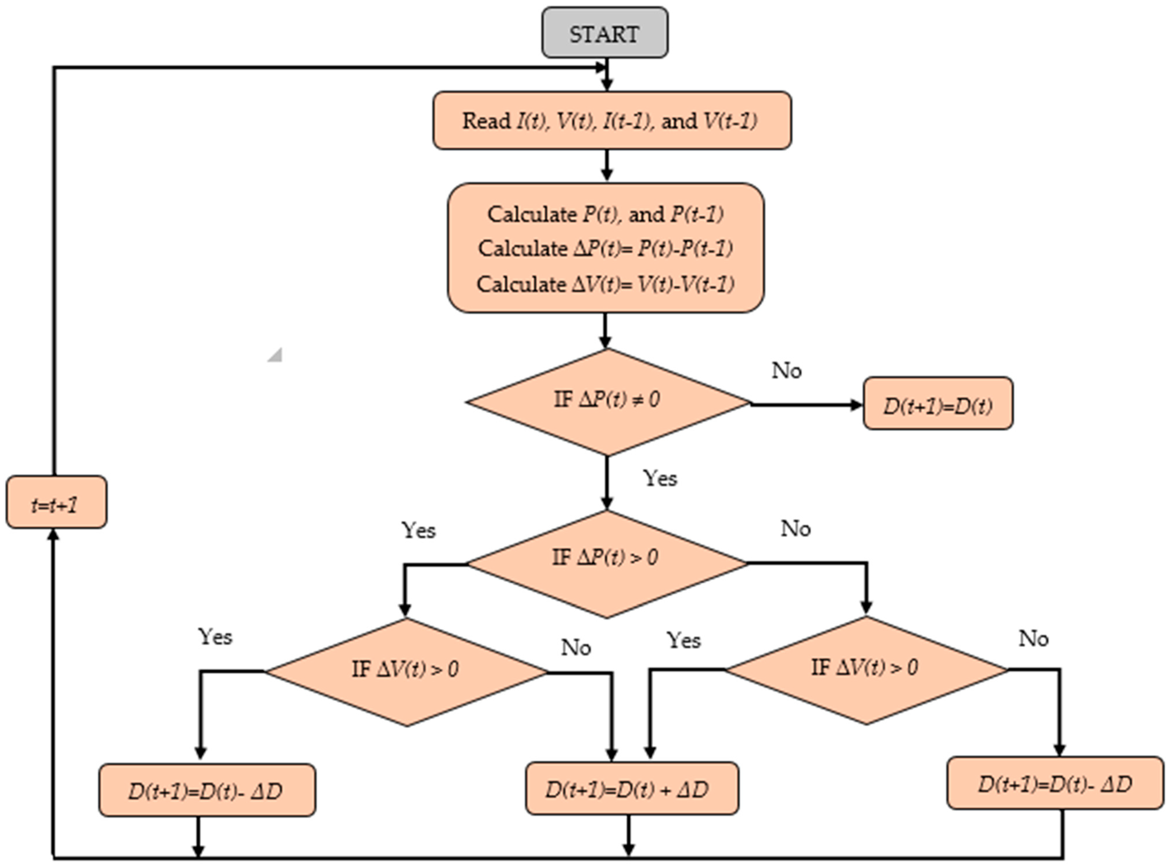
Temperature, pressure, and hydrogen/oxygen partial pressures determine the maximum power point, which in turn determines the optimum working point of PEM fuel cells, which have nonlinear voltage-current characteristics. Implementing maximum power point tracking (MPPT) in PEMFC-based MGs is crucial for adapting to variable operating conditions, maximizing energy harvesting, and improving system efficiency. MPPT algorithms continuously track and adjust the operating point to ensure the system operates at its highest efficiency. To achieve that, PEMFCs usually interface with DC–DC converters to continuously adjust the input resistance to match with the MPP [33,34]. In this study, the PEMFC is interfaced with a boost converter, as depicted in Figure 2, and the Perturb & Observe (P&O) algorithm is applied. The schematic diagram of the P&O algorithm is explained in Figure 3. V(t) and I(t) represent the measured voltage and current of the PEMFC or the PV array at the current sampling time. P(t) denotes the calculated power of the PEMFC or the PV array at the current sampling time. D(t+1) signifies the calculated new duty cycle for the next sampling time. t indicates the measured signals at the current sample time, while t-1 indicates the measured signals at the previous sample time.
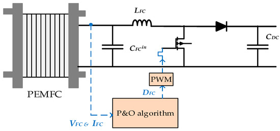
Figure 2.
Structure of the fuel cell system.

Figure 3.
Flowchart of P&O algorithm.
Table 2.
Characteristics of PEM fuel cell used in this study [35,36].
Table 2.
Characteristics of PEM fuel cell used in this study [35,36].
| Parameter | Values |
|---|---|
| 35 | |
| −0.944 | |
| 0.00354 | |
| 2 A cm−1 | |
| L | 0.0178 cm |
2.2. PV Array
This study employs the single-diode-five-parameter equivalent solar cell model to mathematically formulate the PV array. The module current can be calculated as follows [39]:
refers to the output voltage. Iph and stand for the light-generated current and the diode reverse saturation current (amp), with b representing the diode ideality factor. Kb denotes Boltzmann’s constant in J/K (1.3805 × 10⁻²³), while q signifies the electron charge (1.6 × 10⁻¹⁹ Coulombs). and indicate the number of cells connected in series and in parallel, respectively. T denotes the cell operating temperature in Kelvin. Furthermore, the photo current (Iph) of a PV cell is subject to the influence of solar irradiance and temperature, as delineated by the following equation:
is the short-circuit current temperature coefficient at Isc. Rs represents the series resistance of the cell in ohms. It is important to note that the shunt resistance value is typically very large and can be omitted to simplify the analysis.
The performance of a PV array is inherently nonlinear and undergoes changes with fluctuations in solar radiation and temperature. Typically, PV arrays are integrated with a boost converter, as illustrated in Figure 4, serving a dual purpose: tracking the maximum power point on the P–V curve and elevating the PV voltage to align with the specified DC-link voltage limit of the grid-connected inverter. In this study, the P&O algorithm, illustrated in Figure 3, is employed as the MPPT unit for the PV array system.
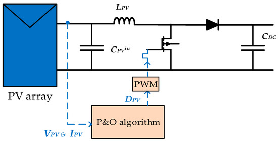
Figure 4.
Structure of PV array system.
2.3. Grid-Connected Inverter
2.3.1. Configuration of the Grid-Connected Inverter
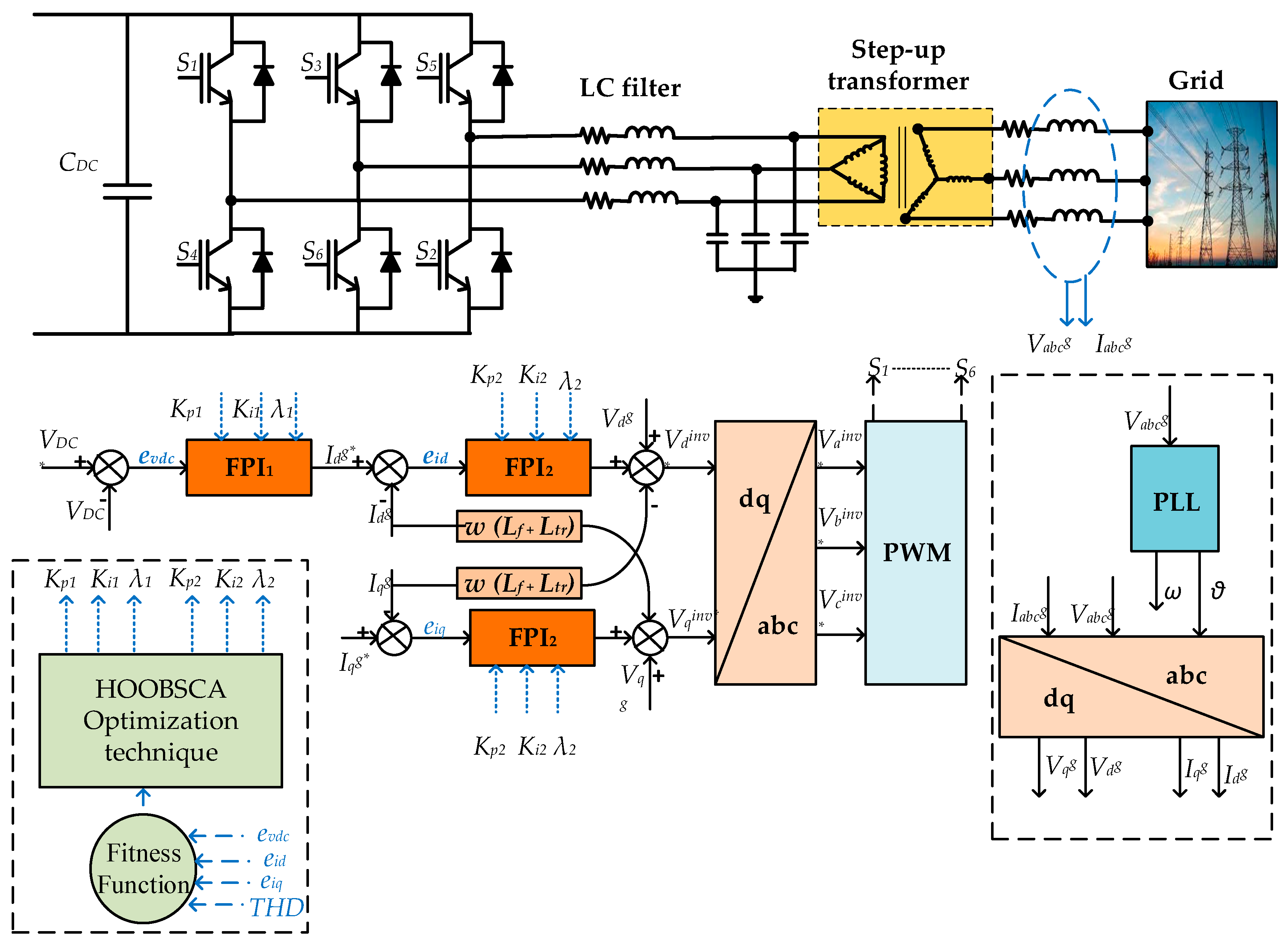
Figure 5 illustrates the core circuit arrangement of a three-phase two-level voltage source converter, enhanced with an LC filter. This setup integrates six switches alongside anti-parallel diodes. One prominent feature of this converter design is its ability to facilitate bidirectional power flow between the DC-side voltage source and the three-phase AC system. Consequently, it demonstrates efficient operation in two distinct modes: as an inverter, converting DC power into AC, or as a rectifier, transforming AC power into DC.

Figure 5.
Control structure of the grid-connected inverter.
To strike a balance between the capacitor size and the DC-voltage ripple, the calculation for determining the size of the DC-link capacitor () is outlined as follows [40]:
where is the inverter switching frequency, and is the maximum DC-link peak-to-peak voltage ripple amplitude.
The LC low-pass filter, functioning as a second-order filter, effectively eliminates higher-order harmonics from the PWM output of the inverter, thereby guaranteeing that the input voltage to the grid assumes a pure sinusoidal form at 60 Hz. To achieve a total harmonic distortion (THD) in the current of less than 5%, the cutoff frequency (Fc) of the low-pass filter is meticulously selected. Typically, Fc is maintained below 1/10th of the inverter switching frequency [41]. The choice of the filter inductance (Lf) holds significant importance, ensuring that the voltage drop across the inductor stays below 3% of the inverter output voltage. The calculation of Lf and Cf can be performed using Equations (13) and (14) [42].
where is the grid frequency, is the output inverter voltage, and is the maximum grid current.
2.3.2. Control of the Grid-Connected Inverter
Voltage-oriented control (VOC) is applied in this work. It is a control strategy extensively employed in three-phase grid-connected inverters, particularly in renewable energy systems where precise regulation of power flow is crucial. The foundation of VOC lies in transforming the three-phase alternating current (AC) quantities into a dq-frame, simplifying control tasks by decoupling the active and reactive power components. The control objectives are then decoupled into active (Pg) and reactive (Qg) power components, each governed by the fractional-order PI controller. The control equations are [29]:
where and are the d- and q-axis components of the grid voltage, respectively. The FPI controller adjusts the DC-link voltage and the inverter output currents to maintain the desired voltage and power factor at the point of common coupling with the grid, as explained in Figure 5. Voltage-oriented control ensures synchronization with the grid voltage, enhancing power quality and stability. Grid voltage feedforward is often incorporated, introducing a feedforward term in the voltage reference equation, further improving the inverter’s response to grid voltage variations. The intricate interplay of these equations ensures effective voltage-oriented control, enabling grid-connected inverters to contribute seamlessly to power systems with renewable energy integration.
Tuning the parameters of a FPI controller is a crucial undertaking in control system design. Meta-heuristic optimization algorithms are frequently employed for this task. This process is typically cast as an optimization problem featuring one or multiple objectives and a set of constraints. The formulated objective function is essential in guiding the optimization process. Specifically, it is structured as follows:
The proposed fitness function (F) encompasses three distinct objectives. The primary objective (F1) is dedicated to minimizing the integral squared error of the DC-link voltage inverter (). Simultaneously, the second objective (F2) focuses on minimizing the integral squared error of the direct () and quadrature () axis currents within the inverter. The third objective (F3) strives to reduce the integral of the total harmonic distortion () in the grid current. Ultimately, these integral squared errors collectively constitute the final objective function (F) implemented in MATLAB r2021a. The corresponding weighting factors, denoted as w1, w2, and w3, are specifically set to 0.4, 0.4, and 0.2, respectively.
The problem constraints revolve around the upper and lower bounds of the FPI’s parameters and the permissible level of THD in the injected signal to the grid, which must be below 5%. These constraints can be derived as follows:
3. The Hybrid One-to-One-Based Optimizer and Sine Cosine Algorithm (HOOBSCA)
The HOOBSCA algorithm embodies a sophisticated fusion of the one-to-one-based optimizer (OOBO) [43], renowned for its effective exploitation capabilities, and the sine cosine algorithm (SCA) [44], known for its effective exploratory features. Through the application of the adopted control technique, the tuning process seamlessly transitions between these two algorithms to pinpoint the optimal solution. Moreover, the hybrid algorithm integrates a set of coefficients, facilitating a harmonious balance between exploitation and exploration. Figure 6 outlines the algorithmic flowchart, and the pseudo-code of HOOBSCA is explained in Algorithm 1.
| Algorithm 1 Pseudo-code of HOOBSCA |
|
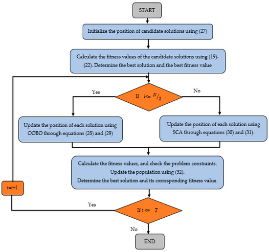
Figure 6.
Flow chart of the proposed HOOBSCA algorithm.
HOOBSCA Steps
The initiation of the HOOBSCA involves initializing the positions of candidate solutions through the following equation:
Within this framework, Xi denotes the present position of the ith solution, with LB and UB serving as indicators for the lower and upper boundaries of the gains, respectively. Additionally, N indicates the population number. The fitness values associated with these positions undergo evaluation through Equation (19).
To facilitate the coordination between the OOBO and the SCA, the population is divided into two equal groups, and the following strategy is applied to update the state of each solution:
- The positions of candidate solutions within the first group are updated using the updating scheme of OOBO, as follows:where signifies the newly suggested position of the ith member in the dth dimension. The term denotes the dth dimension of the selected member guiding the ith member, while represents the objective function value computed based on . The variable is capable of assuming values between 1 and 2. D is the problem dimension. It is worth remarking that the core principle of OOBO in this procedure is to engage every member of the population in the updating process. Consequently, each population member () is randomly selected only once to serve as a guide for another member within the search space.
- The individuals’ positions in the second group are updated using the SCA, as follows:where r2 is a random number from the set [0, 2π], r3 is a random number in the set [0, 2], and r4 is a random number in the set [0, 1]. represents the best solution obtained thus far within the entire population. t is the current iteration, and T is the maximum number of iterations the algorithm executes.
- The population-updating mechanism in the HOOBSCA ensures that a newly suggested status is considered acceptable only if it yields an improvement in the objective function value. In contrast, if the suggested status does not contribute to improvement, it is deemed unacceptable, leading the member to maintain its previous position, as described in Equation (32).
4. Results
The MICCS utilized in this study are depicted in Figure 1. Parameters for the PV array and FC are detailed in Table 1 and Table 2, whereas the specifications for the FC’s converter, the PV’s converters, and the grid-connected inverters are provided in Table 3. The efficacy of the HOOBSCA is assessed in comparison to the OOBO, SCA [45], and the whale optimization algorithm (WOA) in tuning the parameters of the grid inverter control unit under the following case studies:
Table 3.
Specifications of the MICCS converters.
- Between time 0 s and 1 s, solar radiation was at 700 W/m2, subsequently dropping to 400 W/m2 until time 2 s. From time 2 s to 3 s, solar radiation increased to 900 W/m2.
- During the period from time 0 s to 1 s, FC temperature was at 330 K, decreasing to 300 K by time 2 s. Thereafter, the temperature rose again to 330 K from time 2 s to 3 s.
- From time 0 s to 1 s, the battery underwent a constant current charge of 30 A, followed by a discharge with a current of 30 A until time 2 s.
- Between time 1 s and 2 s, the MG supported the grid with a reactive power output of 24.33 kVAR.
- At time 1 s, the first charging station was connected to the MG, absorbing a power load of 6.25 kW. By time 2 s, the second charging station was linked, charging electric vehicles with a cumulative power demand of 12.5 kW.
4.1. Performance of the Proposed HOOBSCA
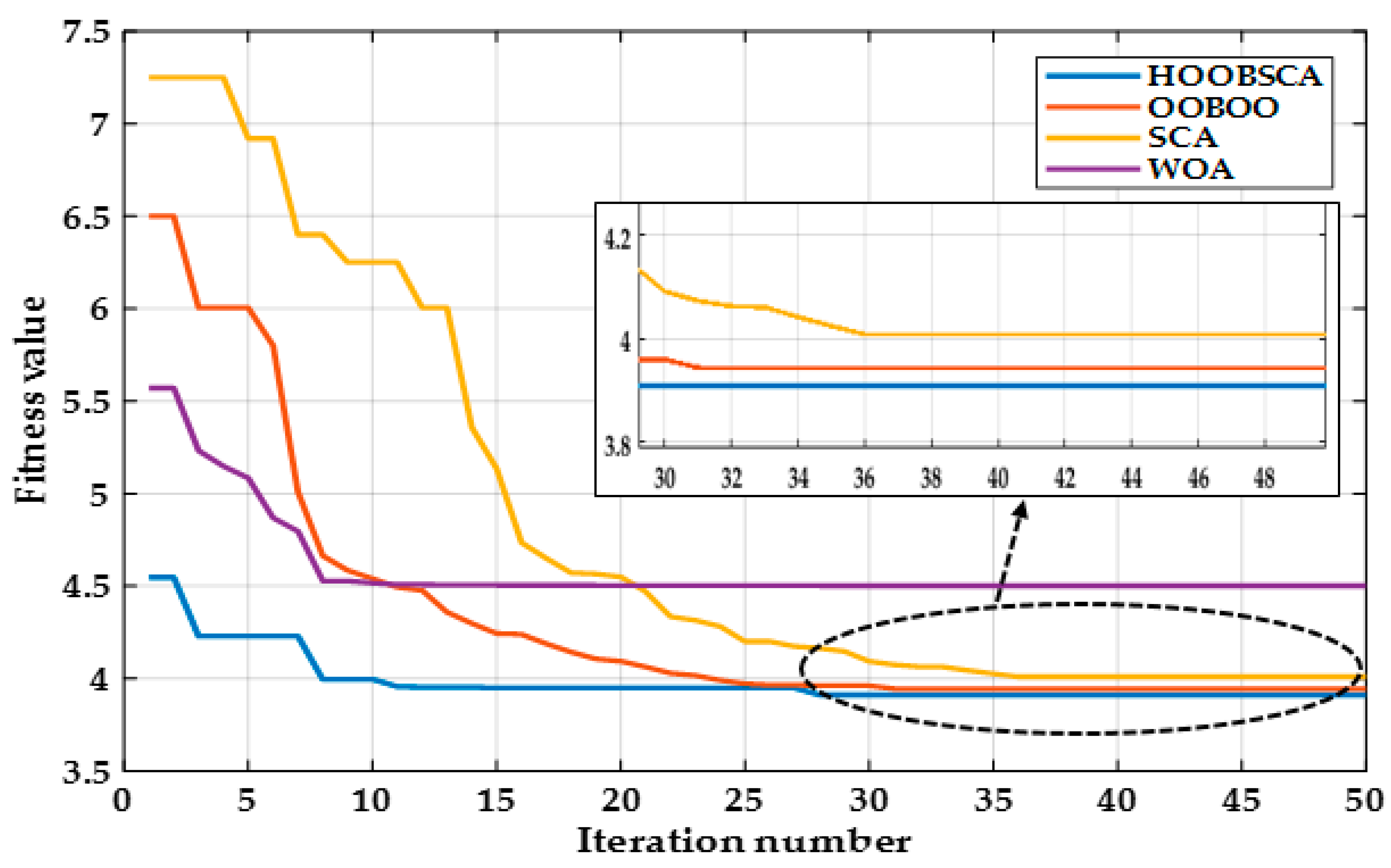
The upper and lower bounds of the controller parameters used in the simulation are presented in Table 4. The results of each algorithm’s estimated parameters are illustrated in Table 5. Figure 7 elucidates the convergence curves of the four algorithms during the tuning of the inverter control unit parameters. Notably, the proposed HOOBSCA exhibited superior performance in achieving high-quality solutions. The best fitness value attained by the proposed optimizer was 3.9109, outperforming the OOBO, SCA, and WOA with best fitness values of 3.9436, 4.0087, and 4.5003, respectively.
Table 4.
Upper and lower bounds of the controller parameters.
Table 5.
Calculated controller parameters and time of computation for each algorithm.
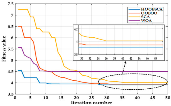
Figure 7.
Convergence curves of HOOBSCA, OOBO, SCA, and WOA in estimating the grid-connected control parameters.
It is noteworthy that the computational time of the algorithm was 9.18 h, compared to 9.27, 8.85, and 9.65 h for OOBO, SCA, and WOA, respectively. While HOOBSCA took slightly longer than SCA by about 3.72% (0.33 h), this difference is negligible given that the tuning strategy is an offline process. The paramount consideration lies in the quality of the obtained solutions, where HOOBSCA demonstrated its superiority.
The obtained results scrutinized the robustness and reliability of the HOOBSCA under various parameter settings and system uncertainties, encompassing diverse operating scenarios. Such analyses offer valuable insights into the algorithm’s applicability for real-world situations, where environmental fluctuations and system dynamics can significantly impact optimization outcomes.
4.2. Performance of the Inverter Control Unit
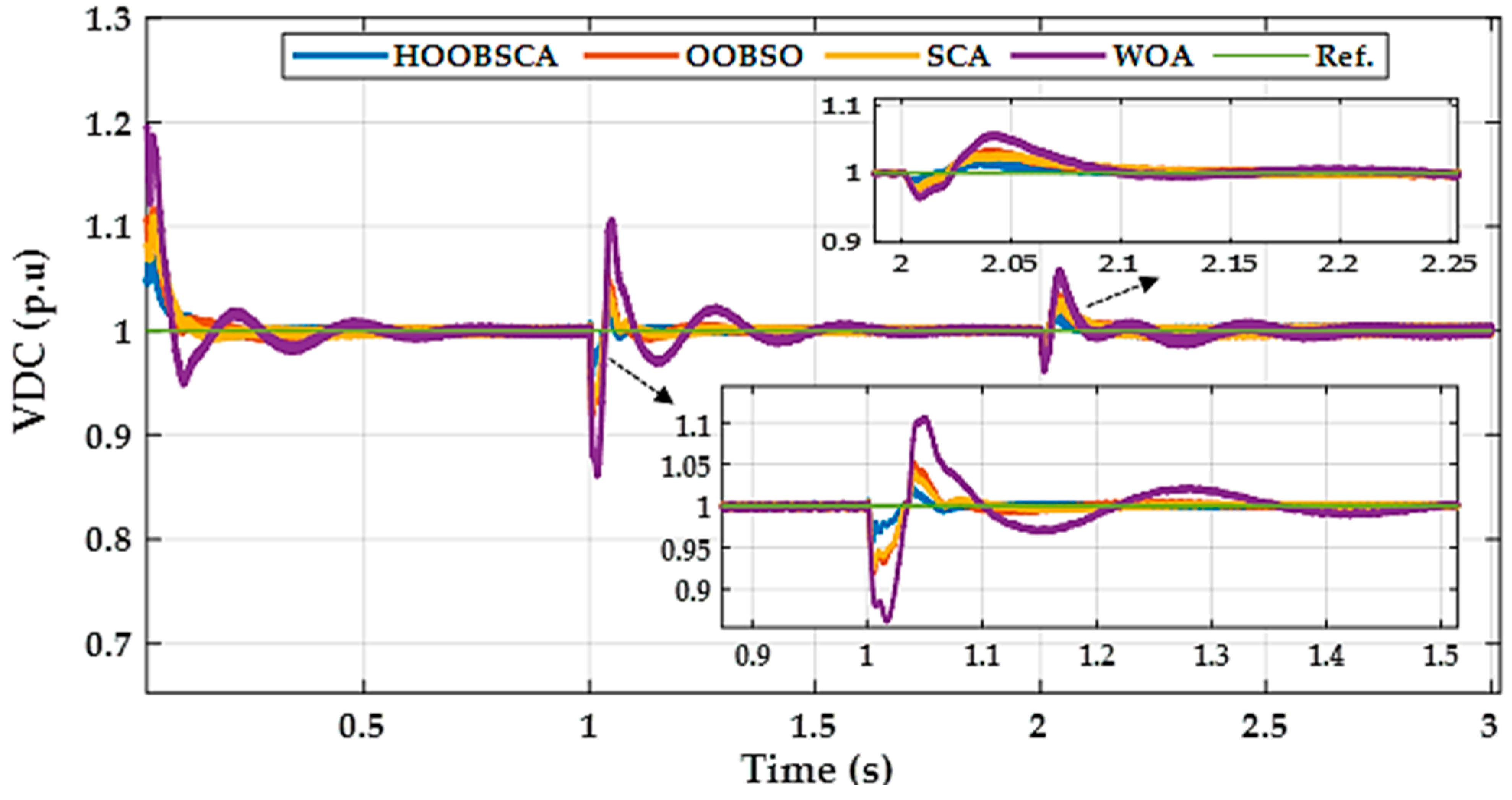
Figure 8 illustrates the response of the DC-link voltage utilizing the four algorithms. The FPI-based HOOBSCA demonstrated greater efficiency than other algorithms, particularly in terms of the percentage of maximum overshoot and settling time. The maximum overshoot with HOOBSCA did not exceed 8.5% across all case studies. In contrast, OOBO exhibited a maximum overshoot of approximately 12.9% in some scenarios, while SCA and WOA recorded values of about 9.5% and 19.9%, respectively. The superiority of HOOBSCA was further evident in achieving the lowest settling time compared to the other algorithms.
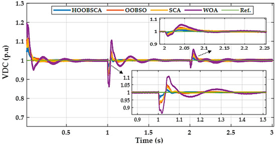
Figure 8.
DC-link voltage responses with HOOBSCA, OOBO, SCA, and WOA.
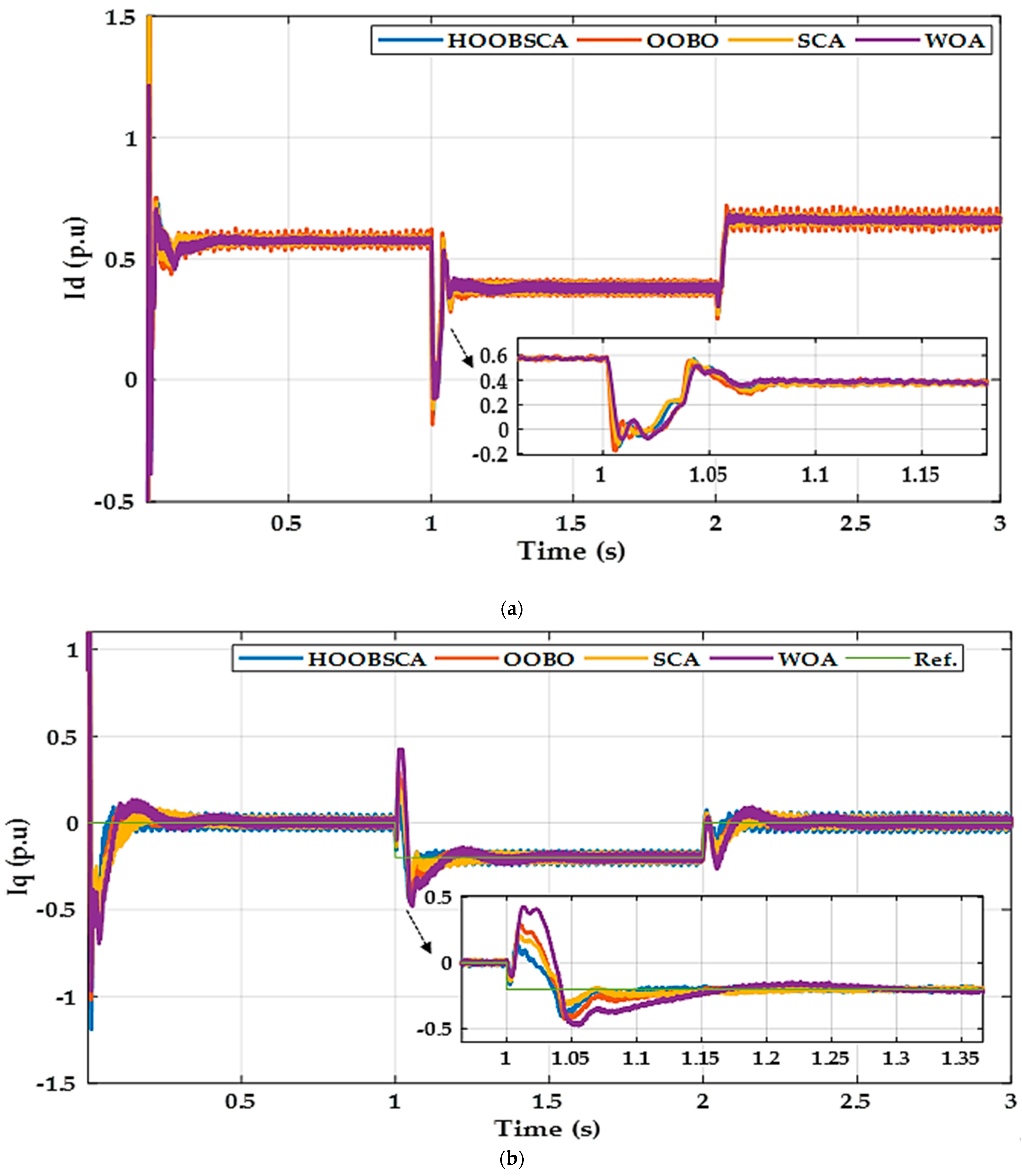
The effectiveness of the current control loop unit can be observed in Figure 9, where Figure 9a showcases the behavior of the d-axis component across various case studies. Notably, the HOOBSCA and WOA algorithms demonstrate exceptional performance in terms of transient response, particularly at the 1 s mark, as well as THD. As depicted in Table 5, the THD values for HOOBSCA and WOA are recorded as 0.82%, while for OOBO and SCA, the THD values stand at 0.91% and 0.86%, respectively.
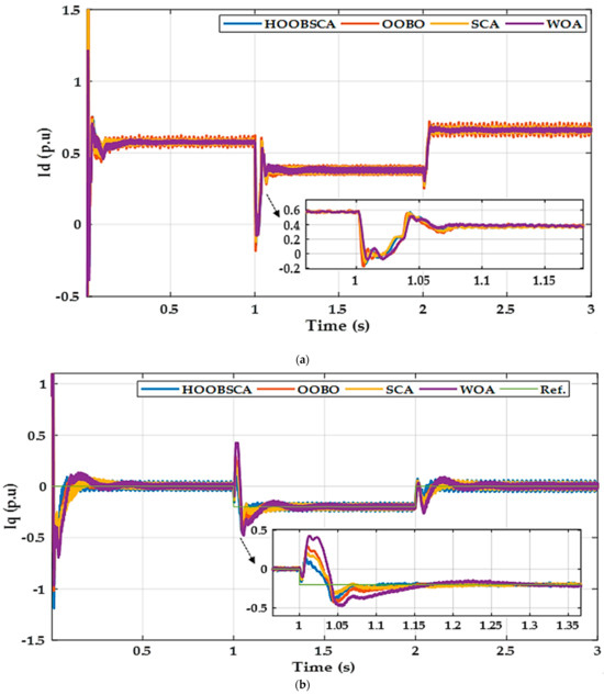
Figure 9.
Grid current of the grid connected inverter with HOOBSCA, OOBO, SCA, and WOA: (a) direct component, and (b) quadrature component.
Figure 9b further highlights the superiority of the HOOBSCA-FPI algorithm. This algorithm effectively showcases a commendable response in the q-axis component of the grid current. To assess the performance of the current control loop, a step change of 0.2 p.u. is introduced in Iqg* at the 2 s mark. The results clearly indicate that the HOOBSCA-FPI algorithm exhibits the least amount of maximum overshooting and boasts the shortest settling time, making it the optimal choice for this application.
The robustness, stability, power quality improvement, adaptability, scalability, and generalizability demonstrated by the proposed inverter control units highlight their pivotal role in tackling the multifaceted challenges inherent in microgrid operation. By ensuring robust performance under diverse operating conditions, including fluctuations in renewable energy generation and dynamic changes in load demand, these control units contribute significantly to the resilience of microgrid systems. Moreover, their ability to enhance power quality metrics, such as minimizing THD in grid currents, signifies a substantial improvement in the reliability and efficiency of electricity delivery, particularly for sensitive equipment and critical infrastructure.
Additionally, the adaptability of these control units enables seamless integration with various microgrid configurations and evolving energy landscapes, ensuring optimal performance and adaptability to future technological advancements. Furthermore, their scalability and generalizability allow for widespread deployment across different scales of microgrid systems, from small-scale residential installations to large-scale industrial or community-based microgrids.
4.3. Performance of the PEMFC and PV Array Control Units
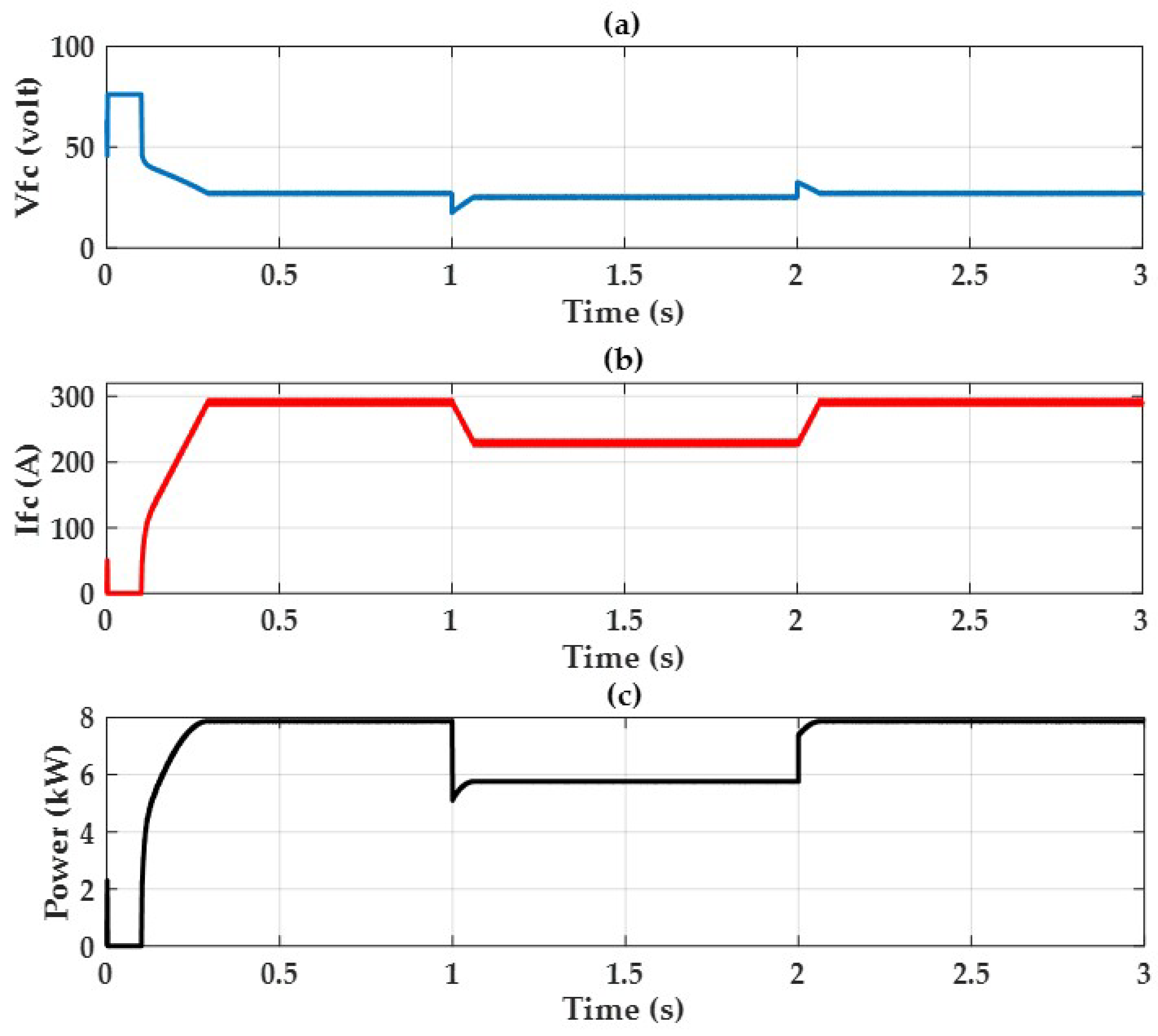
The performance of the PEMFC and PV array systems is elaborated upon in Figure 10 and Figure 11, respectively. In Figure 10, the impact of temperature variation, ranging from 330 K to 300 K at the 1 s mark, and subsequent return to 330 K at the 2 s mark, is depicted through changes in measured fuel cell voltage and current. At a temperature of 330 K, the extracted power amounts to 7.88 kW. However, when the temperature decreases to 300 K, the extracted power diminishes to 5.77 kW.
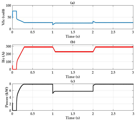
Figure 10.
Performance of the PEMFC system: (a) voltage, (b) current, and (c) the extracted power.
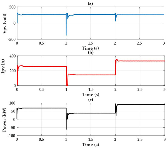
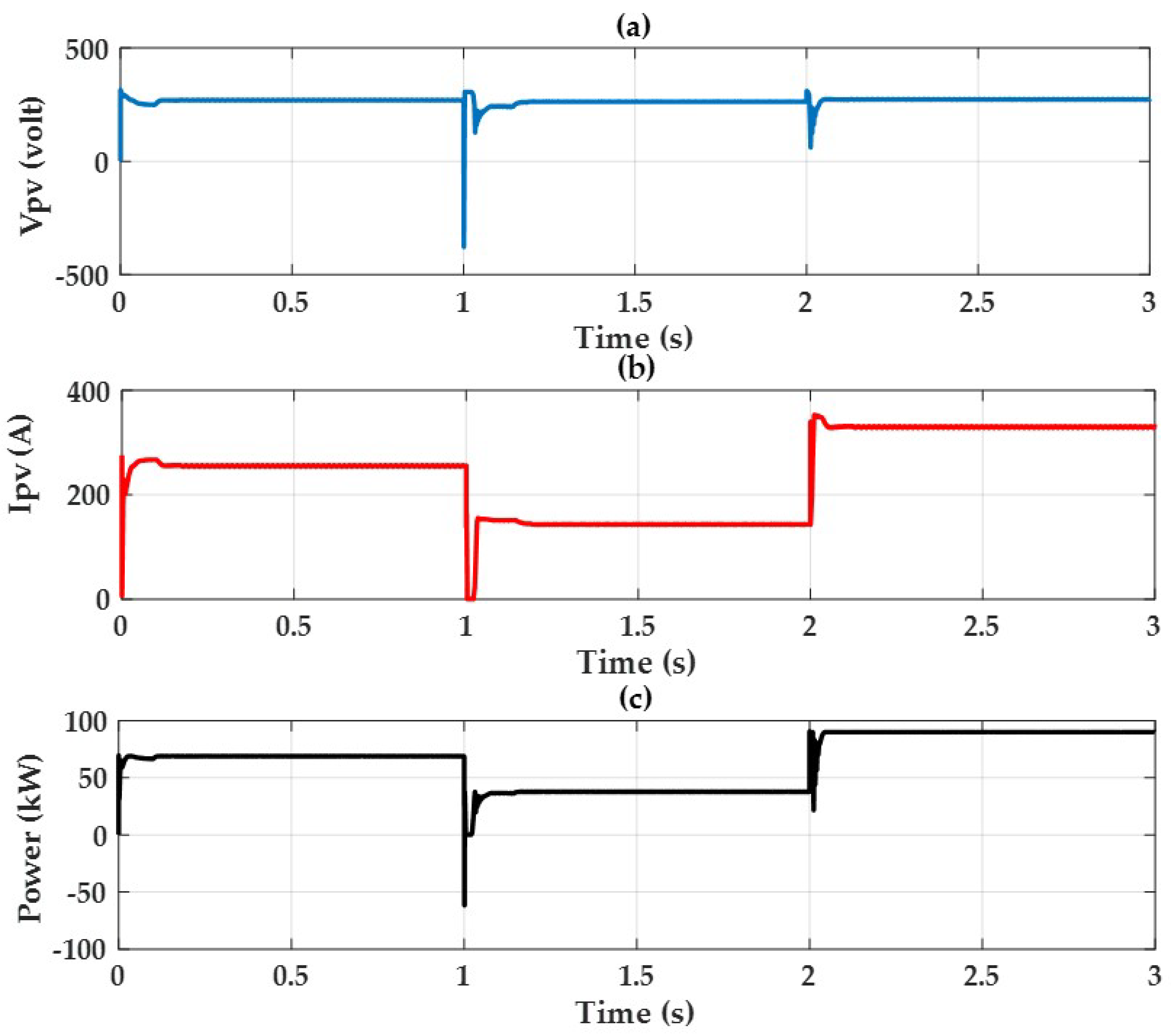
Figure 11.
Performance of the PV system: (a) voltage, (b) current, and (c) the extracted power.
Figure 11 showcases the variations in measured current and voltage of the PV array in response to step changes in solar radiation. Specifically, at the 1 s and 2 s marks, step changes of 700, 400, and 900 W/m2 are applied, while the temperature rests constant at 25 °C. The results demonstrate that the extracted power, under each respective case, amounts to 68.12 kW, 37.76 kW, and 90.07 kW.
4.4. Performance of the Battery Control Unit
Figure 12 illustrates the charging and discharging currents of the battery under the specified operational conditions. Initially, from time 0 s to 1 s, both the PV array and the PEMFC generated substantial power, with no EVs being connected to the charging stations. This enabled the battery to charge at its maximum capacity. Subsequently, between time 1 s and 2 s, the MG encountered its most challenging scenario. During this period, the output power of the PV system and PEMFC decreased due to a decline in solar radiation from 700 W/m2 to 400 W/m2, accompanied by a decrease in the PEMFC temperature to 300 K. Concurrently, the demand from EVs surged to 6.25 kW and the reactive power injected to the grid was 24.33 kVAR, forcing the battery into discharging mode. As time progressed from 2 s to 3 s, the radiation from the PV panels increased to 900 W/m2, and the PEMFC temperature rebounded to 330 K. Notably, during this phase, a second charging station joined the system, resulting in the battery current being held constant at 0 A.
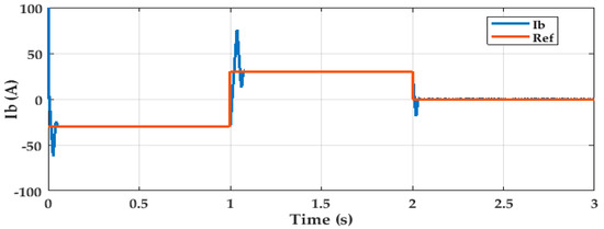
Figure 12.
Battery charging and discharging currents.
5. Conclusions
This paper introduced an effective approach to enhance the performance of MG-integrated charging stations. A new hybrid algorithm, which integrates the one-to-one optimizer with the sine cosine algorithm, was developed to accurately estimate the parameters of the FPI controller. The optimization model was meticulously formulated to target various objectives, including the optimization of the DC-link voltage of the inverter, enhancement of the response of both the direct and quadrature axis currents, and simultaneous improvement of power quality by reducing the total harmonic distortion in the grid current. By incorporating these objectives into the fitness function, the proposed algorithm strives to achieve optimal performance across multiple dimensions, thereby advancing the efficiency and effectiveness of the FPI controller in grid-connected applications.
The application of the HOOBSCA algorithm yielded significant improvements in controller tuning, leading to an enhanced overall performance of the grid-connected inverter compared to other algorithms such as OOBO, SCA, and WOA. The algorithm demonstrated effective exploration of the parameter space, identifying optimal values that minimized error and maximized the inverter’s response accuracy. Through iterative adjustments guided by the HOOBSCA algorithm, the controller achieved a harmonious balance between fast response times and minimal overshoot, crucial for maintaining grid stability.
The proposed HOOBSCA exhibited superior performance in generating high-quality solutions. The best fitness value achieved by the proposed optimizer was 3.9109, outperforming OOBO, SCA, and WOA with best fitness values of 3.9436, 4.0087, and 4.5003, respectively. The HOOBSCA-based FPI successfully improved the response of the DC-link voltage, with a maximum overshooting not exceeding 8.5%, which was 4.4% lower than OOBO, 1% lower than SCA, and 11.4% lower than WOA. When implementing HOOBSCA to regulate the grid current, it demonstrated superior performance in terms of settling time and transient response across various case studies.
The HOOBSCA exhibits limitations due to its longer convergence time compared to the SCA. Addressing this issue requires further investigation through additional studies aimed at refining the algorithm. Moreover, experimental verification with multiple case studies will be essential in future research endeavors to validate and demonstrate the efficacy of the HOOBSCA.
Funding
This study is supported via funding from Prince Sattam bin Abdulaziz University project number (PSAU/2024/R/1445).
Data Availability Statement
The data presented in this study are available on request from the corresponding author.
Conflicts of Interest
The author declares no conflicts of interest.
References
- Trujillo, D.; Torres, E.M.G. Demand Response Due to the Penetration of Electric Vehicles in a Microgrid through Stochastic Optimization. IEEE Lat. Am. Trans. 2022, 20, 651–658. [Google Scholar] [CrossRef]
- Vosoogh, M.; Rashidinejad, M.; Abdollahi, A.; Ghaseminezhad, M. An Intelligent Day Ahead Energy Management Framework for Networked Microgrids Considering High Penetration of Electric Vehicles. IEEE Trans. Ind. Inform. 2020, 17, 667–677. [Google Scholar] [CrossRef]
- Wang, P.; Wang, D.; Zhu, C.; Yang, Y.; Abdullah, H.M.; Mohamed, M.A. Stochastic Management of Hybrid AC/DC Microgrids Considering Electric Vehicles Charging Demands. Energy Rep. 2020, 6, 1338–1352. [Google Scholar] [CrossRef]
- Fatemi, S.; Ketabi, A.; Mansouri, S.A. A Multi-Level Multi-Objective Strategy for Eco-Environmental Management of Electricity Market among Micro-Grids under High Penetration of Smart Homes, Plug-in Electric Vehicles and Energy Storage Devices. J. Energy Storage 2023, 67, 107632. [Google Scholar] [CrossRef]
- Cagnano, A.; De Tuglie, E.; Mancarella, P. Microgrids: Overview and Guidelines for Practical Implementations and Operation. Appl. Energy 2020, 258, 114039. [Google Scholar] [CrossRef]
- Uddin, M.; Mo, H.; Dong, D.; Elsawah, S.; Zhu, J.; Guerrero, J.M. Microgrids: A Review, Outstanding Issues and Future Trends. Energy Strateg. Rev. 2023, 49, 101127. [Google Scholar] [CrossRef]
- Saeed, M.H.; Fangzong, W.; Kalwar, B.A.; Iqbal, S. A Review on Microgrids’ Challenges Perspectives. IEEE Access 2021, 9, 166502–166517. [Google Scholar] [CrossRef]
- Ali, Z.M.; Calasan, M.; Aleem, S.H.E.A.; Jurado, F.; Gandoman, F.H. Applications of Energy Storage Systems in Enhancing Energy Management and Access in Microgrids: A Review. Energies 2023, 16, 5930. [Google Scholar] [CrossRef]
- Mirzaeva, G.; Miller, D. DC and AC Microgrids for Standalone Applications. IEEE Trans. Ind. Appl. 2023, 59, 7908–7918. [Google Scholar] [CrossRef]
- Zolfaghari, M.; Gharehpetian, G.B.; Shafie-khah, M.; Catalão, J.P.S. Comprehensive Review on the Strategies for Controlling the Interconnection of AC and DC Microgrids. Int. J. Electr. Power Energy Syst. 2022, 136, 107742. [Google Scholar] [CrossRef]
- Aljafari, B.; Vasantharaj, S.; Indragandhi, V.; Vaibhav, R. Optimization of DC, AC, and Hybrid AC/DC Microgrid-Based IoT Systems: A Review. Energies 2022, 15, 6813. [Google Scholar] [CrossRef]
- Ali, A.; Mousa, H.H.H.; Shaaban, M.F.; Azzouz, M.A.; Awad, A.S.A. A Comprehensive Review on Charging Topologies and Power Electronic Converter Solutions for Electric Vehicles. J. Mod. Power Syst. Clean Energy 2023, 1–9. [Google Scholar] [CrossRef]
- Khalid, M.R.; Khan, I.A.; Hameed, S.; Asghar, M.S.J.; Ro, J.-S. A Comprehensive Review on Structural Topologies, Power Levels, Energy Storage Systems, and Standards for Electric Vehicle Charging Stations and Their Impacts on Grid. IEEE Access 2021, 9, 128069–128094. [Google Scholar] [CrossRef]
- Chakraborty, S.; Vu, H.-N.; Hasan, M.M.; Tran, D.-D.; Baghdadi, M.E.; Hegazy, O. DC-DC Converter Topologies for Electric Vehicles, Plug-in Hybrid Electric Vehicles and Fast Charging Stations: State of the Art and Future Trends. Energies 2019, 12, 1569. [Google Scholar] [CrossRef]
- Mastoi, M.S.; Zhuang, S.; Munir, H.M.; Haris, M.; Hassan, M.; Usman, M.; Bukhari, S.S.H.; Ro, J.-S. An In-Depth Analysis of Electric Vehicle Charging Station Infrastructure, Policy Implications, and Future Trends. Energy Rep. 2022, 8, 11504–11529. [Google Scholar] [CrossRef]
- Ravindran, M.A.; Nallathambi, K.; Vishnuram, P.; Rathore, R.S.; Bajaj, M.; Rida, I.; Alkhayyat, A. A Novel Technological Review on Fast Charging Infrastructure for Electrical Vehicles: Challenges, Solutions, and Future Research Directions. Alex. Eng. J. 2023, 82, 260–290. [Google Scholar] [CrossRef]
- Heidary, J.; Gheisarnejad, M.; Rastegar, H.; Khooban, M.H. Survey on Microgrids Frequency Regulation: Modeling and Control Systems. Electr. Power Syst. Res. 2022, 213, 108719. [Google Scholar] [CrossRef]
- Hu, J.; Shan, Y.; Guerrero, J.M.; Ioinovici, A.; Chan, K.W.; Rodriguez, J. Model Predictive Control of Microgrids—An Overview. Renew. Sustain. Energy Rev. 2021, 136, 110422. [Google Scholar] [CrossRef]
- Dashtdar, M.; Flah, A.; El-Bayeh, C.Z.; Tostado-Véliz, M.; Al Durra, A.; Abdel Aleem, S.H.E.; Ali, Z.M. Frequency Control of the Islanded Microgrid Based on Optimised Model Predictive Control by PSO. IET Renew. Power Gener. 2022, 16, 2088–2100. [Google Scholar] [CrossRef]
- Suresh, V.; Pachauri, N.; Vigneysh, T. Decentralized Control Strategy for Fuel Cell/PV/BESS Based Microgrid Using Modified Fractional Order PI Controller. Int. J. Hydrogen Energy 2021, 46, 4417–4436. [Google Scholar] [CrossRef]
- AbdelAty, A.M.; Al-Durra, A.; Zeineldin, H.; El-Saadany, E.F. Improving Small-Signal Stability of Inverter-Based Microgrids Using Fractional-Order Control. Int. J. Electr. Power Energy Syst. 2024, 156, 109746. [Google Scholar] [CrossRef]
- Hongesombut, K.; Keteruksa, R. Fractional Order Based on a Flower Pollination Algorithm PID Controller and Virtual Inertia Control for Microgrid Frequency Stabilization. Electr. Power Syst. Res. 2023, 220, 109381. [Google Scholar] [CrossRef]
- Latif, A.; Hussain, S.M.S.; Das, D.C.; Ustun, T.S.; Iqbal, A. A Review on Fractional Order (FO) Controllers’ Optimization for Load Frequency Stabilization in Power Networks. Energy Rep. 2021, 7, 4009–4021. [Google Scholar] [CrossRef]
- Zaheeruddin; Singh, K. Intelligent Fractional-Order-Based Centralized Frequency Controller for Microgrid. IETE J. Res. 2022, 68, 2848–2862. [Google Scholar] [CrossRef]
- Mallesham, G.; Mishra, S.; Jha, A.N. Ziegler-Nichols Based Controller Parameters Tuning for Load Frequency Control in a Microgrid. In Proceedings of the 2011 International Conference on Energy, Automation and Signal, Bhubaneswar, India, 28–30 December 2011; pp. 1–8. [Google Scholar]
- Ali, Z.M.; Ahmed, A.M.; Hasanien, H.M.; Aleem, S.H.E.A. Optimal Design of Fractional-Order PID Controllers for a Nonlinear AWS Wave Energy Converter Using Hybrid Jellyfish Search and Particle Swarm Optimization. Fractal Fract. 2023, 8, 6. [Google Scholar] [CrossRef]
- Ali, M.; Kotb, H.; Aboras, K.M.; Abbasy, N.H. Design of Cascaded Pi-Fractional Order PID Controller for Improving the Frequency Response of Hybrid Microgrid System Using Gorilla Troops Optimizer. IEEE Access 2021, 9, 150715–150732. [Google Scholar] [CrossRef]
- Murugesan, D.; Jagatheesan, K.; Shah, P.; Sekhar, R. Fractional Order PIλDμ Controller for Microgrid Power System Using Cohort Intelligence Optimization. Results Control Optim. 2023, 11, 100218. [Google Scholar]
- Roslan, M.F.; Al-Shetwi, A.Q.; Hannan, M.A.; Ker, P.J.; Zuhdi, A.W.M. Particle Swarm Optimization Algorithm-Based PI Inverter Controller for a Grid-Connected PV System. PLoS ONE 2021, 16, e0259358. [Google Scholar] [CrossRef]
- Hussien, A.M.; Turky, R.A.; Alkuhayli, A.; Hasanien, H.M.; Tostado-Véliz, M.; Jurado, F.; Bansal, R.C. Coot Bird Algorithms-Based Tuning PI Controller for Optimal Microgrid Autonomous Operation. IEEE Access 2022, 10, 6442–6458. [Google Scholar] [CrossRef]
- Ellithy, H.H.; Hasanien, H.M.; Alharbi, M.; Sobhy, M.A.; Taha, A.M.; Attia, M.A. Marine Predator Algorithm-Based Optimal PI Controllers for LVRT Capability Enhancement of Grid-Connected PV Systems. Biomimetics 2024, 9, 66. [Google Scholar] [CrossRef]
- Dhar, R.K.; Merabet, A.; Bakir, H.; Ghias, A.M.Y.M. Implementation of Water Cycle Optimization for Parametric Tuning of PI Controllers in Solar PV and Battery Storage Microgrid System. IEEE Syst. J. 2022, 16, 1751–1762. [Google Scholar] [CrossRef]
- George, S.; Sehgal, N.; Rana, K.P.S.; Kumar, V. A Comprehensive Review on Modelling and Maximum Power Point Tracking of PEMFC. Clean. Energy Syst. 2022, 3, 100031. [Google Scholar] [CrossRef]
- Reddy, K.J.; Sudhakar, N. High Voltage Gain Interleaved Boost Converter with Neural Network Based Mppt Controller for Fuel Cell Based Electric Vehicle Applications. IEEE Access 2017, 6, 3899–3908. [Google Scholar] [CrossRef]
- Rezk, H.; Fathy, A. Performance Improvement of PEM Fuel Cell Using Variable Step-Size Incremental Resistance MPPT Technique. Sustainability 2020, 12, 5601. [Google Scholar] [CrossRef]
- Agwa, A.M.; Alanazi, T.I.; Kraiem, H.; Touti, E.; Alanazi, A.; Alanazi, D.K. MPPT of PEM Fuel Cell Using PI-PD Controller Based on Golden Jackal Optimization Algorithm. Biomimetics 2023, 8, 426. [Google Scholar] [CrossRef]
- Srinivasan, S.; Tiwari, R.; Krishnamoorthy, M.; Lalitha, M.P.; Raj, K.K. Neural Network Based MPPT Control with Reconfigured Quadratic Boost Converter for Fuel Cell Application. Int. J. Hydrogen Energy 2021, 46, 6709–6719. [Google Scholar] [CrossRef]
- Jyotheeswara Reddy, K.; Sudhakar, N. A New RBFN Based MPPT Controller for Grid-Connected PEMFC System with High Step-up Three-Phase IBC. Int. J. Hydrogen Energy 2018, 43, 17835–17848. [Google Scholar] [CrossRef]
- Refaat, M.M.; Atia, Y.; Sayed, M.M.; Fattah, H.A. Adaptive Fuzzy Logic Controller as MPPT Optimization Technique Applied to Grid-Connected PV Systems. In Modern Maximum Power Point Tracking Techniques for Photovoltaic Energy Systems; Springer: Cham, Switzerland, 2020; pp. 247–281. [Google Scholar]
- Vujacic, M.; Hammami, M.; Srndovic, M.; Grandi, G. Analysis of Dc-Link Voltage Switching Ripple in Three-Phase PWM Inverters. Energies 2018, 11, 471. [Google Scholar] [CrossRef]
- Ahmed, K.H.; Finney, S.J.; Williams, B.W. Passive Filter Design for Three-Phase Inverter Interfacing in Distributed Generation. In Proceedings of the 5th International Conference-Workshop Compatibility in Power Electronics, CPE 2007, Gdansk, Poland, 29 May–1 June 2007; Volume XIII, pp. 49–58. [Google Scholar]
- Hojabri, M.; Hojabri, M. Design, Application and Comparison of Passive Filters for Three-Phase Grid-Connected Renewable Energy Systems. ARPN J. Eng. Appl. Sci. 2015, 10, 10691–10697. [Google Scholar]
- Dehghani, M.; Trojovská, E.; Trojovský, P.; Malik, O.P. OOBO: A New Metaheuristic Algorithm for Solving Optimization Problems. Biomimetics 2023, 8, 468. [Google Scholar] [CrossRef]
- Mirjalili, S. SCA: A Sine Cosine Algorithm for Solving Optimization Problems. Knowl.-Based Syst. 2016, 96, 120–133. [Google Scholar] [CrossRef]
- Ismael, S.M.; Aleem, S.H.E.A.; Abdelaziz, A.Y. Optimal Selection of Conductors in Egyptian Radial Distribution Systems Using Sine-Cosine Optimization Algorithm. In Proceedings of the 2017 19th International Middle-East Power Systems Conference, MEPCON 2017—Proceedings, Cairo, Egypt, 19–21 December 2017; Volume 2018, pp. 103–107. [Google Scholar]


Disclaimer/Publisher’s Note: The statements, opinions and data contained in all publications are solely those of the individual author(s) and contributor(s) and not of MDPI and/or the editor(s). MDPI and/or the editor(s) disclaim responsibility for any injury to people or property resulting from any ideas, methods, instructions or products referred to in the content. |
© 2024 by the author. Licensee MDPI, Basel, Switzerland. This article is an open access article distributed under the terms and conditions of the Creative Commons Attribution (CC BY) license (https://creativecommons.org/licenses/by/4.0/).