Convolution Kernel Function and Its Invariance Properties of Bone Fractal Operators

Abstract

This article studies the error function and its invariance properties in the convolutional kernel function of bone fractal operators. Specifically, the following contents are included: (1) demonstrating the correlation between the convolution kernel function and error function of bone fractal operators; (2) focusing on the main part of bone fractal operators: $\sqrt{p+{\alpha }^2}$-type differential operator, discussing the convolutional kernel function image; (3) exploring the fractional-order correlation between the error function and other special functions from the perspective of fractal operators.

1. Introduction

Biomaterial mechanics aims to establish the organic connections between mechanical properties, biological functions, geometric structures, composition, and other factors of biomaterials and reveal the mechanical and physical mechanisms underlying their excellent properties [1]. The different tissues of living organisms, from soft skin, muscles, and whiskers to hard bones, scales, crustacean exoskeletons, etc., all possess comprehensive properties that are suitable for their respective functions. The mystery lies in the orderliness and rationality of the internal structure of biological materials at various levels, from nano to macro, which has a unique effect on their mechanical properties, especially strength and toughness [2,3,4,5,6]. For example, common biological composite materials (such as bones, tendons, and shells) use an integrated “strategy” of alternating softness and hardness, where protein and mineral components each play their respective functions, allowing these natural micro–nano composite structures to achieve good mechanical properties while also possessing various biological functions (such as volume growth) [7,8,9]. In recent years, we have abstracted the multi-level chainlike topology from muscle/ligament fibers [10], nerve fibers [11], and compact bone fibers [12,13] and set up a multi-level micro elastic cavity topology from arterial blood flows [14]. We have built the biological fractal and fractional-order mechanics based on physical components. Surprisingly, these types of problems all exhibit commonalities, namely the common physical fractal space, similar fractal operators, and similar fractional-order mechanics. It can be said that in the above-mentioned biomaterials, fractal operators widely exist, and the idea of fractalization is universally applicable.

The articles [15,16] confirm that bone, as a typical biological composite material, also possesses the aforementioned commonalities. Bones are biomaterials composed of hard substances and brittle substances but simultaneously possess high hardness comparable to minerals and high fracture toughness comparable to proteins [17,18,19]. It has been pointed out in articles [20,21] that the multi-level structure of bone makes mechanical abstraction more difficult. Macroscopically, the bone units in compact bone are the main supporting structures in long bones. In terms of morphology, bone has a chain-like fiber structure, which forms bone units through multi-level self-assembly. However, at each level, it is not simply a chain-like arrangement, including various forms of interlocking, spiral, wrapping, etc. Based on the staggered arrangement pattern of hydroxyapatite in the collagen matrix, a spring–dashpot fractal network with a self-similar topology, named “fractal cell”, is abstracted from the micro/nano-structure of chain-like fibers [10,11]. Based on operational calculus, we built a fractional-order constitutive model of compact bone [12].

In studying the convolutional kernel function of bone fractal operators, we have confirmed that the error function is its core component [13]. This article is a continuation of the previous paper, dedicated to answering a fundamental question: what is the intrinsic expression of the convolutional kernel function in bone fractal operators, and what are the characteristics of bone fractal operators? This article explains the correlation between the convolution kernel function and error function of bone fractal operators, provides the convolutional kernel function image of the $\sqrt{p+{\alpha }^2}$-type differential operator, and preliminarily explores the fractional-order correlation between special functions from the perspective of biological fractal operators. In summary, this article offers a novel approach to building the fractal mechanics of bone and provides a new perspective to establishing the fractional-order correlation between the special functions.

2. Convolution Kernel Function of Bone Fractal Operators

The previous article studied the multi-level structure in bone and abstracted the physical fractal space from the compact bone fibers. From “physical fractal space”, the fractal cells and fractal components have been abstracted, as shown in Figure 1 [12,15]. The constitutive response expression in physical fractal space is

$$\sigma \left(t\right)=T\left(p\right)\epsilon \left(t\right),$$

(1)

where the differential operator $p$ is defined as

$$pg\left(t\right)=\frac{\mathrm{d}g}{\mathrm{d}t}.$$

(2)

Based on the equivalence between fractal components and fractal cells, the algebraic expression of fractal operators $T\left(p\right)$ can be derived:

$$T=\frac{1}{2}\left[T_3\pm \sqrt{{T_3}^2+4\frac{T_1{T}_2{T}_3}{\left(T_1+T_2\right)}}\right].$$

(3)

If the physical component operators are taken as follows:

$$T_1=G_1,T_2=G_2,T_3=G_3{\mu }_{3}p,$$

where both $T_1$ and $T_2$ are elastic elements and $T_3$ is a viscous element, then the main body of the fractal operator becomes

$$\widehat{T}\left(p\right)=p\pm \sqrt{p^2+{\alpha }^{2}p},$$

(4)

where $\alpha =\frac{1}{\sqrt{{\tau }_0}}$ and ${\tau }_0$ is the relaxation time constant.

Interestingly, $\widehat{T}\left(p\right)$ operators have appeared in the hemodynamics of small arteries [14]. Peng et al. have confirmed that the kernel function of the operator $\widehat{T}\left(p\right)$ is a weighted modified Bessel function.

$\widehat{T}\left(p\right)$ operators appeared in both hemodynamics and bone mechanics. In hemodynamic research, Peng et al. considered the operator $\widehat{T}\left(p\right)$ as a whole. Unlike Peng et al., in bone mechanics, Jian et al. separated the quadratic radical term $\sqrt{p^2+{\alpha }^{2}p}$ in the operator $\widehat{T}\left(p\right)$ and studied it separately [13]:

$$\stackrel{⌢}{T}\left(p\right)=\sqrt{p^2+{\alpha }^{2}p}=\sqrt{p}\sqrt{p+{\alpha }^2}.$$

(5)

The quadratic radical operator $\stackrel{⌢}{T}\left(p\right)$ is decomposed into the product of two 1/2-order differential operators $\sqrt{p}$ and $\sqrt{p+{\alpha }^2}$. ${\alpha }^2$ is equivalent to characteristic frequency. The intention of this article is based on the following consideration: if given $\alpha =i\lambda$, the operator $\sqrt{p+{\alpha }^2}$ can be extended to the operator $\sqrt{p-{\lambda }^2}$. In Equation (5), $\sqrt{p}$ is a classical fractional-order operator. The operator $\sqrt{p+{\alpha }^2}$ is also a classical fractional-order operator, which is widely used in heat conduction problems, viscoelastic problems, and hemodynamics. However, recently, we have noticed that $\sqrt{p+{\alpha }^2}$ operators have very beautiful invariance properties. These beautiful invariance properties possess excellent transferability: they are passed on not only to the quadratic radical operator $\stackrel{⌢}{T}\left(p\right)$, but also to numerous operators constructed by $\sqrt{p+{\alpha }^2}$. Therefore, $\sqrt{p+{\alpha }^2}$ operators deserve special attention. In fact, as long as the properties of the operator $\sqrt{p+{\alpha }^2}$ are clarified, the properties of the quadratic radical operator $\stackrel{⌢}{T}\left(p\right)$ in Equation (5) will be clear.

In Courant’s work [22], the operator $\sqrt{p+{\alpha }^2}$ acting on the Heaviside unit step function $\eta \left(t\right)$ generates a convolutional kernel function $h\left(t\right)$:

$$h\left(t\right)=\sqrt{p+{\alpha }^2}\eta (t).$$

With the help of the displacement theorem

$$\sqrt{p+{\alpha }^2}\eta (t)=e^{-{\alpha }^{2}t}\sqrt{p}\left[e^{{\alpha }^{2}t}\eta \left(t\right)\right],$$

the expression for the kernel function $h\left(t\right)$ can be written as

$$h\left(t\right)=\sqrt{p+{\alpha }^2}\eta (t)=\frac{e^{-{\alpha }^{2}t}}{\sqrt{\pi }}\frac{\mathrm{d}}{\mathrm{d}t}{\displaystyle \underset{0}{\overset{t}{\int }}\frac{e^{{\alpha }^2\tau }}{\sqrt{t-\tau }}}\mathrm{d}\tau .$$

(6)

In Equation (6), ${\displaystyle \underset{0}{\overset{t}{\int }}\frac{e^{{\alpha }^2\tau }}{\sqrt{t-\tau }}}\mathrm{d}\tau$ is the characteristic integral of the convolutional kernel function of bone fractal operators in the physical fractal space. It comes from $\sqrt{p}\left[e^{{\alpha }^{2}t}\eta \left(t\right)\right]$, where $e^{{\alpha }^2\tau }$ is the exponential term brought by the displacement theorem. This is very common in the viscoelastic response of biomaterials [10]. $\frac{1}{\sqrt{t-\tau }}$ comes from the convolutional kernel function of the operator $\sqrt{p}$.

As mentioned above, the fractional-order differential operator $\sqrt{p+{\alpha }^2}$ and its characteristic integral ${\displaystyle \underset{0}{\overset{t}{\int }}\frac{e^{{\alpha }^2\tau }}{\sqrt{t-\tau }}}\mathrm{d}\tau$ belong to classical analysis. In Courant’s work [22], the characteristic integral term ${\displaystyle \underset{0}{\overset{t}{\int }}\frac{e^{{\alpha }^2\tau }}{\sqrt{t-\tau }}}\mathrm{d}\tau$ is considered as the core component of the kernel function $h\left(t\right)$. However, reference [22] ignored the internal structure of characteristic integral. Recently, Jian et al. noticed that the characteristic integral actually includes an error function. This means that the kernel function $h\left(t\right)$ of the operator $\sqrt{p+{\alpha }^2}$ includes an error function. In this way, it is necessary to deeply understand the operator $\sqrt{p+{\alpha }^2}$ from the perspective of the error function. This constitutes the motivation of this article.

3. Error Function in Kernel Function of Bone Fractal Operators

This section demonstrates the correlation between the convolution kernel function and error function of bone fractal operators and discusses the convolutional kernel function image.

The characteristic integral ${\displaystyle \underset{0}{\overset{t}{\int }}\frac{e^{{\alpha }^2\tau }}{\sqrt{t-\tau }}}\mathrm{d}\tau$ in Equation (6) is examined:

$${\displaystyle \underset{0}{\overset{t}{\int }}\frac{e^{{\alpha }^2\tau }}{\sqrt{t-\tau }}}\mathrm{d}\tau =e^{{\alpha }^{2}t}{\displaystyle \underset{0}{\overset{t}{\int }}\frac{e^{{\alpha }^2(\tau -t)}}{\sqrt{t-\tau }}}\mathrm{d}\tau =e^{{\alpha }^{2}t}{\displaystyle \underset{\sqrt{{\alpha }^{2}t}}{\overset{0}{\int }}\frac{e^{-x^2}}{\frac{x}{\sqrt{{\alpha }^2}}}}\frac{2x}{-{\alpha }^2}\mathrm{d}x=\frac{2e^{{\alpha }^{2}t}}{\sqrt{{\alpha }^2}}{\displaystyle \underset{0}{\overset{\sqrt{{\alpha }^{2}t}}{\int }}{e}^{-x^2}\mathrm{d}x}.$$

According to the definition of the error function,

$${\displaystyle \underset{0}{\overset{\sqrt{{\alpha }^{2}t}}{\int }}{e}^{-x^2}\mathrm{d}x=}\frac{\sqrt{\pi }}{2}\mathrm{erf}\left(\sqrt{{\alpha }^{2}t}\right).$$

Therefore, the characteristic integral is transformed into

$${\displaystyle \underset{0}{\overset{t}{\int }}\frac{e^{{\alpha }^2\tau }}{\sqrt{t-\tau }}}\mathrm{d}\tau =\frac{\sqrt{\pi }}{\sqrt{{\alpha }^2}}{e}^{{\alpha }^{2}t}\mathrm{erf}\left(\sqrt{{\alpha }^{2}t}\right).$$

(7)

It can be seen that the characteristic integral is composed of two functions; one is the error function $\mathrm{erf}\left(\sqrt{{\alpha }^{2}t}\right)$, and the other is the exponential function $e^{{\alpha }^{2}t}$. So, the convolutional kernel function in Equation (6) can be expressed as

$$h\left(t\right)=\sqrt{p+{\alpha }^2}\eta (t)=\frac{e^{-{\alpha }^{2}t}}{\sqrt{{\alpha }^2}}\frac{\mathrm{d}}{\mathrm{d}t}\left[e^{{\alpha }^{2}t}\mathrm{erf}\left(\sqrt{{\alpha }^{2}t}\right)\right].$$

(8)

Note the following differential properties of the error function:

$$\frac{\mathrm{d}}{\mathrm{d}t}\left[\mathrm{erf}(\gamma t)\right]=\frac{2\gamma e^{-{\gamma }^2{t}^2}}{\sqrt{\pi }}.$$

(9)

Equation (9) shows that the first-order differential operator $p=\frac{\mathrm{d}}{\mathrm{d}t}$ transforms the non-elementary error function into the elementary negative exponential function. Equation (9) shows the correlation between the error function and the negative exponential function. Of course, this result is trivial because the error function is originally obtained by integrating a negative exponential function.

Equations (8) and (9) are derived simultaneously:

$$h\left(t\right)=\sqrt{p+{\alpha }^2}\eta (t)=\alpha \mathrm{erf}(\sqrt{{\alpha }^{2}t})+\frac{e^{-{\alpha }^{2}t}}{\sqrt{\pi t}}.$$

(10)

This is the analytical form $\sqrt{p+{\alpha }^2}\eta (t)$ exported in the previous article [13].

Equation (10) indicates that the kernel function $h\left(t\right)$ of the fractional-order differential operator $\sqrt{p+{\alpha }^2}$ can be expressed as the sum of the error function $\mathrm{erf}(\sqrt{{\alpha }^{2}t})$ and the weighted negative exponential function $\frac{e^{-{\alpha }^{2}t}}{\sqrt{\pi t}}$, where the former is a non-elementary function and the latter is an elementary function. The kernel function $\sqrt{p+{\alpha }^2}\eta (t)$ can be decomposed into the sum of elementary and non-elementary functions; this phenomenon has not been noticed in the past.

Note that the error function is bounded; when $t\to 0$, $\mathrm{erf}\left(t\right)\to 0$; when $t\to \pm \infty$, $\mathrm{erf}\left(t\right)\to \pm 1$. However, when $t\to 0$, $\frac{e^{-t}}{\sqrt{t}}\to \infty$; when $t\to \infty$, $\frac{e^{-t}}{\sqrt{t}}\to 0$. Therefore, we obtain

$$\underset{t\to 0}{\lim }h\left(t\right)=\underset{t\to 0}{\lim }\left[\alpha \mathrm{erf}(\sqrt{{\alpha }^{2}t})+\frac{e^{-{\alpha }^{2}t}}{\sqrt{\pi t}}\right]\to \infty$$

and

$$\underset{t\to \infty }{\lim }h\left(t\right)=\underset{t\to \infty }{\lim }\left[\alpha \mathrm{erf}(\sqrt{{\alpha }^{2}t})+\frac{e^{-{\alpha }^{2}t}}{\sqrt{\pi t}}\right]\to \alpha .$$

The function image of Equation (10) when $\sqrt{{\tau }_0}=0.1 \mathrm{s},0.2 \mathrm{s},0.4 \mathrm{s},0.8 \mathrm{s},1.6 \mathrm{s}$, namely $\alpha =10,5,2.5,1.25,0.625$, is shown in Figure 2.

As the relaxation time constant ${\tau }_0$ increases, $\alpha$ decreases and $h\left(t\right)$ correspondingly decays (when $t\to \infty$). As shown in Figure 2, if $\sqrt{{\tau }_0}=0.1 \mathrm{s}$, when $t\to \infty$, $h\left(t\right)\to \frac{1}{\sqrt{{\tau }_0}}=\alpha =10$; when $t\to 0$, $h\left(t\right)\to \infty$. Similarly, if $\sqrt{{\tau }_0}=1.6 \mathrm{s}$, when $t\to \infty$, $h\left(t\right)\to \frac{1}{\sqrt{{\tau }_0}}=\alpha =0.625$; when $t\to 0$, $h\left(t\right)\to \infty$. Therefore, the kernel function $h\left(t\right)$ is essentially an analytical function that decays over time $t$, and the core parameter that determines the speed of decay is the relaxation time constant ${\tau }_0=\frac{1}{{\alpha }^2}$. From this, it can be seen that the most common convolutional kernel function in bone fractal operators (Equation (10)) has the same trend of variation as the Dirac pulse function $\delta \left(t\right)$. This is a very interesting phenomenon that also explains why $\sqrt{p+{\alpha }^2}$ operators widely exist in many disciplines.

4. Error Function in Inverse Operator Kernel Function of Bone Fractal Operators

Surprisingly, the error function appears not only in the kernel function of the fractional-order differential operator $\sqrt{p+{\alpha }^2}$, but also in the kernel function of the fractional-order integral operator $\frac{1}{\sqrt{p+{\alpha }^2}}$. Note that the fractional-order integral operator $\frac{1}{\sqrt{p+{\alpha }^2}}$ is the inverse operator of the fractional-order differential operator $\sqrt{p+{\alpha }^2}$.

Mikusinski’s work [23] provides the following expression:

$$\frac{1}{\sqrt{p+{\alpha }^2}}\eta \left(t\right)=\frac{\mathrm{erf}\left(\sqrt{{\alpha }^{2}t}\right)}{\alpha }.$$

(11)

The kernel function of the operator $\frac{1}{\sqrt{p+{\alpha }^2}}$ is the error function. Note that, unlike operator $\sqrt{p+{\alpha }^2}$, the kernel function of the inverse operator $\frac{1}{\sqrt{p+{\alpha }^2}}$ does not include negative exponential functions at all, meaning that it can only be characterized by non-elementary functions. From this, it can be seen that the inverse operators $\sqrt{p+{\alpha }^2}$ and $\frac{1}{\sqrt{p+{\alpha }^2}}$, although closely related, also possess profound differences: both depend on the error function, but one contains the elementary function and the other does not. Interestingly, if $\sqrt{p+{\alpha }^2}$ is combined with $\frac{1}{\sqrt{p+{\alpha }^2}}$, a considerable amount of information can be exported.

By combining Equations (11) and (10), we have

$$\left(\sqrt{p+{\alpha }^2}-\frac{{\alpha }^2}{\sqrt{p+{\alpha }^2}}\right)\eta \left(t\right)=\frac{e^{-{\alpha }^{2}t}}{\sqrt{\pi t}}.$$

By simplifying the above equation, we have

$$\frac{p}{\sqrt{p+{\alpha }^2}}\eta \left(t\right)=\frac{e^{-{\alpha }^{2}t}}{\sqrt{\pi t}}.$$

(12)

Equation (12) indicates that in Courant’s work [22], the kernel function of the calculus operator $\frac{p}{\sqrt{p+{\alpha }^2}}$ is the elementary function $\frac{e^{-{\alpha }^{2}t}}{\sqrt{\pi t}}$.

With operator $p$ acting on both ends of Equation (11) simultaneously, we have

$$\frac{p}{\sqrt{p+{\alpha }^2}}\eta \left(t\right)=p\left[\frac{\mathrm{erf}\left(\sqrt{{\alpha }^{2}t}\right)}{\alpha }\right].$$

(13)

By comparing Equations (13) and (12), we have

$$p\left[\frac{\mathrm{erf}\left(\sqrt{{\alpha }^{2}t}\right)}{\alpha }\right]=\frac{e^{-{\alpha }^{2}t}}{\sqrt{\pi t}}.$$

(14)

Equation (14) is completely equivalent to Equation (9). Comparing Equation (9), it can be seen that the error function possesses a beautiful property: as a non-elementary function, its first-order derivative is actually an elementary function.

5. Correlation between Error Function and Bessel Function

From a historical perspective, the origin of the error function is different from that of the Bessel function, and there is no correlation between the two. However, with the help of the inverse operator $\frac{1}{\sqrt{p+{\alpha }^2}}$ of the fractional-order operator $\sqrt{p+{\alpha }^2}$, we can see the interesting correlation between these two types of special functions.

Equation (11) acts on the fractional-order operator $\sqrt{p}$ at both ends simultaneously:

$$\begin{array}{l}\sqrt{p}\frac{1}{\sqrt{p+{\alpha }^2}}\eta \left(t\right)=\sqrt{p}\frac{\mathrm{erf}\left(\sqrt{{\alpha }^{2}t}\right)}{\alpha }\\ =\frac{\mathrm{d}}{\mathrm{d}t}{\displaystyle {\int }_0^t\frac{1}{\sqrt{\pi \left(t-\tau \right)}}\frac{\mathrm{erf}\left(\sqrt{{\alpha }^2\tau }\right)}{\alpha }\mathrm{d}\tau }=e^{-\frac{{\alpha }^{2}t}{2}}{\overline{J}}_0\left(\frac{{\alpha }^{2}t}{2}\right).\end{array}$$

(15)

Equation (15) indicates that the 1/2-order fractional differential of the error function $\frac{\mathrm{erf}\left(\sqrt{{\alpha }^{2}t}\right)}{\alpha }$, namely the operator $\sqrt{p}$ acting on $\frac{\mathrm{erf}\left(\sqrt{{\alpha }^{2}t}\right)}{\alpha }$, generates a weighted Bessel function $e^{-\frac{{\alpha }^{2}t}{2}}{\overline{J}}_0\left(\frac{{\alpha }^{2}t}{2}\right)$ with a negative power exponent function. It should be emphasized that the overbar notation of the Bessel functions is not conventional [24]. Equation (15) can be further expressed as

$$\frac{p}{\stackrel{⌢}{T}\left(p\right)}\eta \left(t\right)=\frac{p}{\sqrt{p}\sqrt{p+{\alpha }^2}}\eta \left(t\right)=\sqrt{p}\frac{\mathrm{erf}\left(\sqrt{{\alpha }^{2}t}\right)}{\alpha }=e^{-\frac{{\alpha }^{2}t}{2}}{\overline{J}}_0\left(\frac{{\alpha }^{2}t}{2}\right).$$

(16)

Equation (16) shows that the input signal is a non-elementary function $\frac{\mathrm{erf}\left(\sqrt{{\alpha }^{2}t}\right)}{\alpha }$, and through the action of fractional-order differential operator $\sqrt{p}$, the output signal becomes the product of an elementary function and a non-elementary function, namely $e^{-\frac{{\alpha }^{2}t}{2}}{\overline{J}}_0\left(\frac{{\alpha }^{2}t}{2}\right)$.

Equation (16) can also be understood in this way: the 0-order Bessel function [24] can be represented by the fractional derivative of the error function.

Equation (16) reveals the correlation between the error function and the 0-order corrected Bessel function. This result is quite unexpected: the error function and Bessel function come from completely different mathematical and physical problems. On the surface, it is difficult to see any connection between the two. However, with the help of the operator $\sqrt{p+{\alpha }^2}$, the deep dependency relationship between the two has been revealed.

Comparing Equations (14) and (16), it can be seen that the integer-order differential operator $p$ acts on a non-elementary function $\frac{\mathrm{erf}\left(\sqrt{{\alpha }^{2}t}\right)}{\alpha }$, resulting in an elementary function $\frac{e^{-{\alpha }^{2}t}}{\sqrt{\pi t}}$; the 1/2-order fractional differential operator $\sqrt{p}$ acts on a non-elementary function $\frac{\mathrm{erf}\left(\sqrt{{\alpha }^{2}t}\right)}{\alpha }$, resulting in a non-elementary function $e^{-\frac{{\alpha }^{2}t}{2}}{\overline{J}}_0\left(\frac{{\alpha }^{2}t}{2}\right)$. It can be seen that the non-elementary property of the Bessel function comes from the fractional-order differential operator $\sqrt{p}$.

We can understand Equation (16) from the perspective of fractional-order differential equations. Consider the following fractional-order differential equation:

$$\sqrt{p}f\left(t\right)=e^{-\frac{{\alpha }^{2}t}{2}}{\overline{J}}_0\left(\frac{{\alpha }^{2}t}{2}\right).$$

(17)

Equation (17) has a specific solution:

$$f\left(t\right)=\frac{\mathrm{erf}\left(\sqrt{{\alpha }^{2}t}\right)}{\alpha }.$$

(18)

Equation (18) shows that the error function can be considered as a solution to the fractional-order differential equation (Equation (17)). From Equations (16) and (18), it can be seen that the error function only depends on the 0-order corrected Bessel function and negative power exponent function.

6. Correlation between Error Function and Bessel Function in Quadratic Radical Operators

As shown in Equation (5), there is a quadratic radical operator $\stackrel{⌢}{T}\left(p\right)=\sqrt{p}\sqrt{p+{\alpha }^2}$ in bone fractal operators. The inverse operator $\frac{1}{\stackrel{⌢}{T}\left(p\right)}$ of this operator has already appeared in Equation (16). For the sake of comparison, look at the quadratic radical operator $\stackrel{⌢}{T}\left(p\right)=\sqrt{p}\sqrt{p+{\alpha }^2}$ from a different perspective. Start directly from $\sqrt{p+{\alpha }^2}\eta (t)$ (Equation (9)). Equation (10) acts on the fractional-order operator $\sqrt{p}$ at both ends simultaneously:

$$\stackrel{⌢}{T}\left(p\right)\eta (t)=\sqrt{p}\sqrt{p+{\alpha }^2}\eta (t)=\sqrt{p}\left(\alpha \mathrm{erf}(\sqrt{{\alpha }^2\tau })+\frac{e^{-{\alpha }^2\tau }}{\sqrt{\pi \tau }}\right).$$

(19)

The right side of Equation (19) is changed into

$$\begin{array}{l}\sqrt{p}\left(\alpha \mathrm{erf}(\sqrt{{\alpha }^2\tau })+\frac{e^{-{\alpha }^2\tau }}{\sqrt{\pi \tau }}\right)=\frac{1}{\sqrt{\pi }}\frac{\mathrm{d}}{\mathrm{d}t}{\displaystyle \underset{0}{\overset{t}{\int }}\frac{\left(\alpha \mathrm{erf}(\sqrt{{\alpha }^2\tau })+\frac{e^{-{\alpha }^2\tau }}{\sqrt{\pi \tau }}\right)}{\sqrt{t-\tau }}}\mathrm{d}\tau \\ =\frac{\mathrm{d}}{\mathrm{d}t}\left({\displaystyle \underset{0}{\overset{t}{\int }}\frac{\left(\alpha \mathrm{erf}(\sqrt{{\alpha }^2\tau })\right)}{\sqrt{\pi \left(t-\tau \right)}}}+\frac{e^{-{\alpha }^2\tau }}{\pi \sqrt{\left(t-\tau \right)\tau }}\right)\mathrm{d}\tau \\ ={\alpha }^2{e}^{-\frac{{\alpha }^{2}t}{2}}{\overline{J}}_0\left[\frac{{\alpha }^{2}t}{2}\right]+\frac{1}{2}{\alpha }^2{e}^{-\frac{{\alpha }^{2}t}{2}}\left\{-{\overline{J}}_0\left[\frac{{\alpha }^{2}t}{2}\right]+{\overline{J}}_1\left[\frac{{\alpha }^{2}t}{2}\right]\right\}+\delta \left(t\right)\\ =\frac{1}{2}{\alpha }^2{e}^{-\frac{{\alpha }^{2}t}{2}}\left({\overline{J}}_0\left[\frac{{\alpha }^{2}t}{2}\right]+{\overline{J}}_1\left[\frac{{\alpha }^{2}t}{2}\right]\right)+\delta \left(t\right).\end{array}$$

(20)

Combining Equations (19) and (20), the final result is

$$\begin{array}{l}\stackrel{⌢}{T}\left(p\right)\eta (t)=\sqrt{p}\sqrt{p+{\alpha }^2}\eta (t)=\sqrt{p}\left(\alpha \mathrm{erf}(\sqrt{{\alpha }^{2}t})+\frac{e^{-{\alpha }^{2}t}}{\sqrt{\pi t}}\right)\\ =\frac{1}{2}{\alpha }^2{e}^{-\frac{{\alpha }^{2}t}{2}}\left({\overline{J}}_0\left[\frac{{\alpha }^{2}t}{2}\right]+{\overline{J}}_1\left[\frac{{\alpha }^{2}t}{2}\right]\right)+\delta \left(t\right).\end{array}$$

(21)

Equation (21) shows that the input signal is the sum of elementary and non-elementary functions, and through the action of the fractional-order differential operator $\sqrt{p}$, the output signal becomes the product of elementary and non-elementary functions, which is summed with the Dirac pulse function. The limit of this kernel function at $t\to 0$ is $\frac{{\alpha }^2}{2}$, as shown in Figure 2, which is a slowly decaying function.

We can examine Equation (21) from the perspective of fractional-order differential equations. Consider the following 1/2-order differential equation:

$$\sqrt{p}f\left(t\right)=\frac{1}{2}{\alpha }^2{e}^{-\frac{{\alpha }^{2}t}{2}}\left({\overline{J}}_0\left[\frac{{\alpha }^{2}t}{2}\right]+{\overline{J}}_1\left[\frac{{\alpha }^{2}t}{2}\right]\right)+\delta \left(t\right).$$

(22)

Comparing Equations (21) and (22), it can be seen that the equation has the following special solution:

$$f\left(t\right)=\alpha \mathrm{erf}(\sqrt{{\alpha }^{2}t})+\frac{e^{-{\alpha }^{2}t}}{\sqrt{\pi t}}.$$

(23)

Equation (23) shows that the error function is the solution of a 1/2-order differential equation. From this, it can be seen that the error function differs from various special functions: the former is the solution of fractional-order differential equations, while the latter is the solution of integer-order differential equations.

On the surface, Equation (21) shows the correlation between the error function, the 0th-order and 1st-order modified Bessel functions, and the Dirac pulse function. In fact, since the error function is only related to the 0th-order corrected Bessel function (see Equation (16)), the 1st-order corrected Bessel function and the Dirac pulse function should mainly come from the fractional-order derivative of the negative power exponential function. The evidence is as follows:

By combining Equations (21) and (16), the following two equations can be obtained:

$$\begin{array}{l}\left[\stackrel{⌢}{T}\left(p\right)-{\alpha }^2\frac{p}{\stackrel{⌢}{T}\left(p\right)}\right]\eta \left(t\right)=\left[\sqrt{p}\sqrt{p+{\alpha }^2}-{\alpha }^2\frac{p}{\sqrt{p}\sqrt{p+{\alpha }^2}}\right]\eta \left(t\right)\\ =\frac{p^2}{\sqrt{p}\sqrt{p+{\alpha }^2}}\eta \left(t\right)=\sqrt{p}\left(\frac{e^{-{\alpha }^{2}t}}{\sqrt{\pi t}}\right)\\ =\frac{1}{2}{\alpha }^2{e}^{-\frac{{\alpha }^{2}t}{2}}\left(-{\overline{J}}_0\left[\frac{{\alpha }^{2}t}{2}\right]+{\overline{J}}_1\left[\frac{{\alpha }^{2}t}{2}\right]\right)+\delta \left(t\right),\end{array}$$

(24)

$$\begin{array}{l}\left[\stackrel{⌢}{T}\left(p\right)-\frac{1}{2}{\alpha }^2\frac{p}{\stackrel{⌢}{T}\left(p\right)}\right]\eta \left(t\right)=\left[\sqrt{p}\sqrt{p+{\alpha }^2}-\frac{1}{2}{\alpha }^2\frac{p}{\sqrt{p}\sqrt{p+{\alpha }^2}}\right]\eta (t)\\ =\sqrt{p}\left(\frac{1}{2}\mathrm{erf}(\sqrt{{\alpha }^{2}t})+\frac{e^{-{\alpha }^{2}t}}{\sqrt{\pi t}}\right)=\frac{1}{2}{\alpha }^2{e}^{-\frac{{\alpha }^{2}t}{2}}{\overline{J}}_1\left[\frac{{\alpha }^{2}t}{2}\right]+\delta \left(t\right).\end{array}$$

(25)

The following discussion focuses on Equation (24), and readers can interpret Equation (25) on their own. Equation (24) shows that the fractional-order derivative of the weighted negative exponential function $\frac{e^{-{\alpha }^{2}t}}{\sqrt{\pi t}}$ leads to the derivation of the 0th-order and 1st-order modified Bessel functions. Equation (24) reveals the correlation between the negative power exponential function, the 0th-order modified Bessel function, the 1st-order modified Bessel function, and the Dirac pulse function. It can be determined that the first-order modified Bessel function and the Dirac pulse function do indeed come from the fractional-order derivative of the negative power exponential function.

Equation (25) can also be understood in this way: similar to the 0th-order Bessel function, the 1st-order Bessel function can also be represented by the fractional-order derivative of the error function due to the existence of the following recursive formula between different-order Bessel functions:

$${\overline{J}}_{n-1}\left(t\right)+{\overline{J}}_{n+1}\left(t\right)=2t^{-1}{\overline{J}}_n\left(t\right),$$

$${\overline{J}}_{n-1}\left(t\right)-{\overline{J}}_{n+1}\left(t\right)=2p{\overline{J}}_n\left(t\right).$$

The recursive formula shows that higher-order Bessel functions can be represented by lower-order Bessel functions and their derivatives. Now, both 0th-order and 1st-order Bessel functions can be characterized by fractional-order derivatives of the error function. Therefore, based on the recursive formula, we can assert that higher-order Bessel functions can also be characterized by fractional-order derivatives of the error function. In other words, the solutions to the Bessel equation can be represented by the fractional-order derivative of the error function.

The correlation between the negative power exponent function, the Dirac pulse function, and the 0th-order and 1st-order modified Bessel functions is quite unexpected because there is an insurmountable gap between elementary and non-elementary functions. Now, with the help of fractional-order calculus, the gap has been filled.

Note that in Equation (24), the input signal is an elementary function, but after the action of the fractional-order differential operator $\sqrt{p}$, the output signal becomes a non-elementary function. Fractional-order differentiation seems to strengthen the non-elementary property of functions.

Based on Equation (24), consider the following fractional-order differential equation:

$$\sqrt{p}f\left(t\right)=\frac{1}{2}{\alpha }^2{e}^{-\frac{{\alpha }^{2}t}{2}}\left(-{\overline{J}}_0\left[\frac{{\alpha }^{2}t}{2}\right]+{\overline{J}}_1\left[\frac{{\alpha }^{2}t}{2}\right]\right)+\delta \left(t\right).$$

(26)

Comparing Equations (24) and (26), it can be seen that Equation (26) has a specific solution:

$$f\left(t\right)=\frac{e^{-{\alpha }^{2}t}}{\sqrt{\pi t}}.$$

(27)

Equation (27) shows that the negative exponential function is also a solution to fractional-order differential equations.

7. Correlation between Error Function and Gamma Function

With the help of the operator $\sqrt{p+{\alpha }^2}$ and quadratic radical operator $\stackrel{⌢}{T}\left(p\right)$, the correlation between the error function and the Bessel function was revealed in the previous article [13] and the above sections. This section will use the quadratic radical operator $\stackrel{⌢}{T}\left(p\right)$ and error function to further reveal the correlation between the error function and Gamma functions.

We focus on the integral properties of the error function. It is easy to export the following equation:

$${\displaystyle \underset{0}{\overset{t}{\int }}\mathrm{erf}(\sqrt{{\alpha }^2\tau })\mathrm{d}\tau }=\frac{1}{{\alpha }^2}\left[\frac{\sqrt{{\alpha }^{2}t}{e}^{-{\alpha }^{2}t}}{\sqrt{\pi }}+\left(-\frac{1}{2}+{\alpha }^{2}t\right)\mathrm{erf}(\sqrt{{\alpha }^{2}t})\right].$$

(28)

In Equation (9), the differentiation of the error function is an elementary function; in Equation (28), the integration of the error function is still related to the error function.

When using the Frobenius method to solve the Bessel equation [25,26], the Gamma function is usually introduced; it is defined as

$$\Gamma \left(z\right)={\displaystyle \underset{0}{\overset{\infty }{\int }}{t}^{z-1}{e}^{-t}\mathrm{d}t}.$$

The Gamma function is a very important special function in mathematics and has wide applications in many fields [27]. For example, in probability theory and statistics, the Gamma function is commonly used to normalize the probability density function [28]; in quantum mechanics, the Gamma function appears in the wave function of particles; in engineering, the Gamma function is commonly used to calculate problems such as integration, probability, and signal processing [29,30].

We note that the integration of the error function is related not only to itself (Equation (28)), but also to the Gamma function:

$${\displaystyle \underset{0}{\overset{t}{\int }}\mathrm{erf}(\sqrt{{\alpha }^2\tau })\mathrm{d}\tau }=t\mathrm{erf}(\sqrt{{\alpha }^{2}t})+\frac{1}{2{\alpha }^2}\left[\frac{2\Gamma \left(\frac{3}{2},{\alpha }^{2}t\right)}{\sqrt{\pi }}-1\right].$$

(29)

Here, the definition of the incomplete Gamma function is

$$\Gamma \left(a,z\right)={\displaystyle \underset{z}{\overset{\infty }{\int }}{t}^{a-1}{e}^{-t}}\mathrm{d}t.$$

It should be noted that there are no discontinuous branch lines in $\Gamma \left(z\right)$, and there is a discontinuous branch line from $-\infty$ to 0 in the complex plane of $\Gamma \left(a,z\right)$.

By combining Equations (28) and (29), it can be concluded that

$$\mathrm{erf}\left(\sqrt{{\alpha }^{2}t}\right)+\frac{2\Gamma \left(\frac{3}{2},{\alpha }^{2}t\right)}{\sqrt{\pi }}=1+\frac{2\sqrt{{\alpha }^{2}t}{e}^{-{\alpha }^{2}t}}{\sqrt{\pi }}.$$

(30)

There is such a simple algebraic identity between the Gamma function and the error function.

The left-hand end of Equation (30) is the algebraic sum of two non-elementary functions, but the right-hand end is an elementary function. This means that the non-elementary parts of the error function and gamma function can cancel each other out, leaving behind the elementary parts.

8. Correlation between Gamma Function and Bessel Function

Equation (30) shows the correlation between the Gamma function and the error function. Note that there is a correlation between the error function and the Bessel function (Equation (16)). So, using the error function as a bridge, the Bessel function can be associated with the Gamma function.

Substituting Equation (30) into Equation (16), we have

$$\begin{array}{l}\frac{p}{\stackrel{⌢}{T}\left(p\right)}\eta \left(t\right)=\frac{p}{\sqrt{p}\sqrt{p+{\alpha }^2}}\eta \left(t\right)=\sqrt{p}\frac{\mathrm{erf}\left(\sqrt{{\alpha }^{2}t}\right)}{\alpha }\\ =\frac{1}{\alpha \sqrt{\pi }}\sqrt{p}\left[\sqrt{\pi }+2\sqrt{{\alpha }^{2}t}{e}^{-{\alpha }^{2}t}-2\Gamma \left(\frac{3}{2},{\alpha }^{2}t\right)\right]=e^{-\frac{{\alpha }^{2}t}{2}}{\overline{J}}_0\left(\frac{{\alpha }^{2}t}{2}\right).\end{array}$$

(31)

Equation (31) shows that there is a transformation between the Bessel function and the Gamma function, which is controlled by the fractional-order differential operator $\sqrt{p}$.

Equation (31) indicates that the kernel function of the irrational fraction operator $\frac{p}{\stackrel{⌢}{T}\left(p\right)}$ can be represented by different non-elementary functions: it can be characterized by the error function, Gamma function, or Bessel function.

Note that in Equation (31), the 0th-order Bessel function appears, while in Equation (25), the 1st-order Bessel function appears. The simultaneous Equations (30) and (25) can be derived as follows:

$$\begin{array}{l}\left[\stackrel{⌢}{T}\left(p\right)-\frac{1}{2}{\alpha }^2\frac{p}{\stackrel{⌢}{T}\left(p\right)}\right]=\left[\sqrt{p}\sqrt{p+{\alpha }^2}-\frac{1}{2}{\alpha }^2\frac{p}{\sqrt{p}\sqrt{p+{\alpha }^2}}\right]\eta (t)\\ =\sqrt{p}\left\{\frac{\alpha }{2\sqrt{\pi }}\left[\sqrt{\pi }+2\sqrt{{\alpha }^{2}t}{e}^{-{\alpha }^{2}t}-2\Gamma \left(\frac{3}{2},{\alpha }^{2}t\right)\right]+\frac{e^{-{\alpha }^{2}t}}{\sqrt{\pi t}}\right\}\\ =\frac{1}{2}{\alpha }^2{e}^{-\frac{{\alpha }^{2}t}{2}}{\overline{J}}_1\left[\frac{{\alpha }^{2}t}{2}\right]+\delta \left(t\right).\end{array}$$

(32)

Equation (32) indicates that there is also a profound correlation between the first-order Bessel function, the Dirac pulse function, and the Gamma function. Note that both the 0th-order and 1st-order Bessel functions can be expressed as fractional-order derivatives of the Gamma function. By using the recursive formula of the Bessel function, it can be inferred that higher-order Bessel functions are also associated with the Gamma function and can be expressed as fractional-order derivatives of the Gamma function. That is to say, the solutions to the Bessel equation can be represented by the fractional-order derivative of the Gamma function.

The solution of the Bessel equation can be represented by either the fractional-order derivative of the error function or the fractional-order derivative of the Gamma function. The equivalent form of the solution indicates that the expression of the solution to the Bessel equation is not unique.

The kernel function of the irrational calculus operator $\left[\stackrel{⌢}{T}\left(p\right)-\frac{1}{2}{\alpha }^2\frac{p}{\stackrel{⌢}{T}\left(p\right)}\right]$ can be a fractional-order derivative of the Gamma function or a weighted first-order Bessel function.

We can also look at Equation (31) or Equation (32) from the perspective of fractional-order differential equations:

$$\frac{1}{\alpha \sqrt{\pi }}\sqrt{p}f\left(t\right)=e^{-\frac{{\alpha }^{2}t}{2}}{\overline{J}}_0\left(\frac{{\alpha }^{2}t}{2}\right).$$

(33)

Comparing Equation (31) and Equation (33), it can be seen that Equation (33) has a special solution:

$$f\left(t\right)=\sqrt{\pi }+2\sqrt{{\alpha }^{2}t}{e}^{-{\alpha }^{2}t}-2\Gamma \left(\frac{3}{2},{\alpha }^{2}t\right).$$

(34)

Obviously, the Gamma function is the main component of the solution to fractional-order differential equations (Equation (33)).

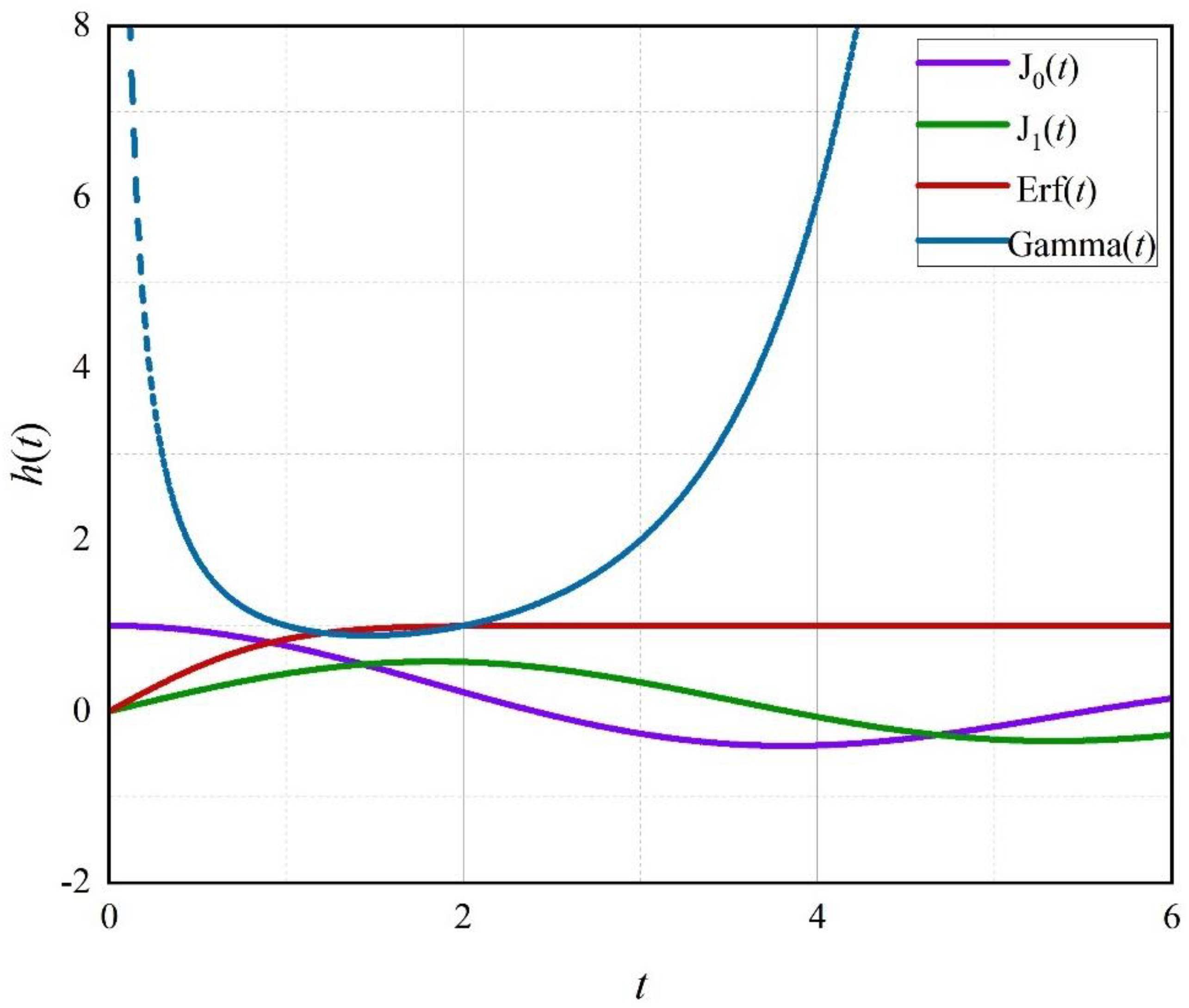
Once again, it should be emphasized that the origins of the error function, Gamma function, and Bessel function are completely different. The difference in function images is significant (as shown in Figure 3). We really cannot see any correlation from the graph. Now, with the help of fractal operators, we have established profound intrinsic correlations between the three types of non-elementary functions, which are seemingly unrelated. In future work, we will derive the fractional-order correlations between various special functions from the perspective of bone fractal operators, including the error function, Gamma function, Bessel function, MeijerG function, and hypergeometric function.

9. Conclusions

$\sqrt{p+{\alpha }^2}$ and $\stackrel{⌢}{T}\left(p\right)=\sqrt{p}\sqrt{p+{\alpha }^2}$ are indeed unusual fractional-order operators. They possess rich invariance properties, and their inverse operators, namely $\frac{1}{\sqrt{p+{\alpha }^2}}$ and $\frac{1}{\sqrt{p}\sqrt{p+{\alpha }^2}}$, also possess rich invariance properties. Based on the invariance properties of the above operators, we discover a profound intrinsic correlation between the error function, Bessel function, Gamma function, and weighted exponential function. It can be said that using fractal operators not only expands the boundaries of mechanics, but also deepens our understanding of non-elementary functions and fractional-order calculus.

It should be noted that the fractal operators in this article are all non-integer-order operators. Such non-integer-order operators are suitable tools for characterizing non-localization effects. Therefore, the following concept will be further strengthened: the mechanics in physical fractal space is the non-localized mechanics, the non-integer-order mechanics, and the mechanics controlled by non-elementary functions.