
Statistical Study of the Bias and Precision for Six Estimation Methods for the Fractal Dimension of Randomly Rough Surfaces

 ,
,  , ,
, ,
Abstract
:1. Introduction
2. Methods
2.1. Surface Simulation and Characterisation as a Random Process
2.2. Surface Generation
2.3. Box Counting Methods
2.4. Triangular Prism Method
2.5. Detrended Fluctuation
2.6. Roughness–Length Method
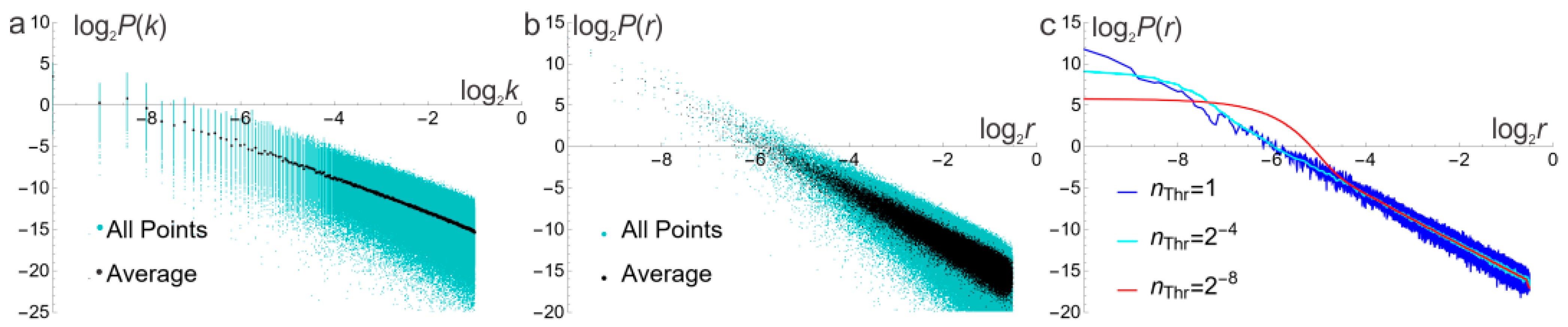
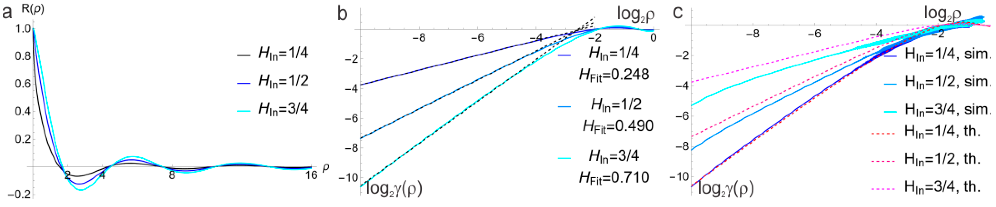
2.7. Power Spectral Density and Related Functions
2.8. Tuning of the PSA
2.9. Tuning of the SFA
3. Simulations and Results
3.1. Simulation Scheme
3.2. Data Analysis
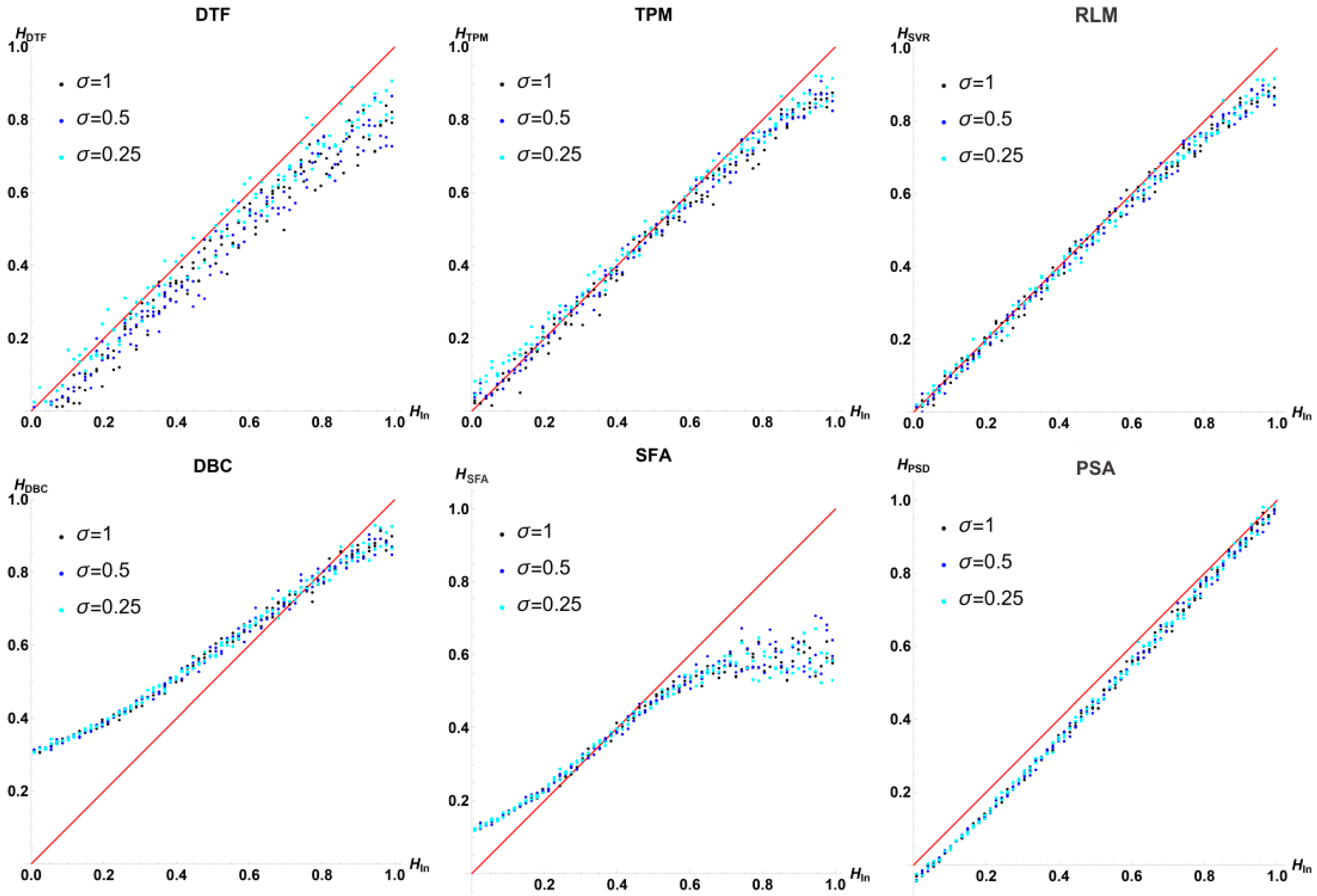
3.3. Results for
3.4. Results for
4. Discussion
4.1. Bias, Dispersion, and Precision
4.2. Computational Efficiency
4.3. Information Efficiency
4.4. Effect of Vertical Scaling and Resolution
4.5. Effect of the Surface Generation Algorithm
5. Conclusions
Supplementary Materials
Author Contributions
Funding
Data Availability Statement
Acknowledgments
Conflicts of Interest
Abbreviations
| PS | Power spectrum |
| PSD | Power spectral density |
| ANOVA | Analysis of variance |
| WM | Weierstrass–Mandelbrot |
| FFT | Fast Fourier transform |
| IFT | Inverse fast Fourier transform |
| DTF | Discrete Fourier transform |
| Fourier transform | |
| Inverse Fourier transform | |
| Real part | |
| Imaginary part | |
| Ceiling | |
| Expected value | |
| Gamma function | |
| 1 | generalised hypergeometric function |
| x, y, z, | Coordinates in physical domain |
| Points in physical domain | |
| Radius in physical domain | |
| Fractal function on a square domain | |
| Density function in physical space | |
| variance of | |
| Longest wavelength in physical space | |
| Shortest wavelength in physical space | |
| k | Wave vector in the frequency domain |
| k, l | Coordinates in the frequency domain |
| Points in the frequency domain | |
| r | Radial coordinate in the frequency domain |
| upper cut-off radius in frequency domain | |
| upper cut-off radius in frequency domain | |
| D | Fractal dimension |
| H | Hurst exponent |
| C | Arbitrary normalisation constant |
| G | Fractal roughness (WM) |
| Lacunarity (WM) | |
| Power spectrum as a function of r | |
| Autocorrelation of | |
| Structure function of | |
| Input value of standard deviation | |
| Input value of H for simulation | |
| Surface generation method (generic) | |
| WM | Weierstrass–Mandelbrot (method) |
| MP | Random midpoint (method) |
| FT | Fourier transform (method) |
| Set of random numbers (generic) | |
| M, N | Number of terms in WM |
| matrix of Gaussian values | |
| Random phase angles in WM | |
| Method to determine H (generic) | |
| BCM | Box counting methods (generic) |
| DBC | Differential box counting (method) |
| DTF | Detrended fluctuation (method) |
| TPM | Triangular prism method |
| RLM | Roughness–length method |
| PSA | Power spectrum analysis (method) |
| SFA | Structure–function analysis (method) |
| a | Size of square sub-domain |
| Number of sub-domains | |
| over entire domain | |
| Maximum of in sub-domain i. | |
| Minimum of in sub-domain i. | |
| Regression function for DTF | |
| Residual variance for sub-domain size a | |
| parameters | |
| Total surface determined in TPM | |
| Autocorrelation for method | |
| Treshold radius for low-pass filter | |
| (dispersion) | |
| (precision) | |
| R2 | Coefficient of determination |
References
- Longuet-Higgins, M.S. The statistical analysis of a random, moving surface. Philos. Trans. R. Soc. Lond. Ser. A Math. Phys. Sci. 1957, 249, 321–387. [Google Scholar] [CrossRef]
- Longuet-Higgins, M.S. Statistical properties of an isotropic random surface. Philos. Trans. R. Soc. Lond. Ser. A Math. Phys. Sci. 1957, 250, 157–174. [Google Scholar] [CrossRef]
- Whitehouse, D.J.; Archard, J.F. The properties of random surfaces of significance in their contact. Proc. R. Soc. Lond. Ser. A. Math. Phys. Sci. 1970, 316, 97–121. [Google Scholar] [CrossRef]
- Pfeifer, P. Fractal dimension as working tool for surface-roughness problems. Appl. Surf. Sci. 1984, 18, 146–164. [Google Scholar] [CrossRef]
- Pfeifer, P.; Wu, Y.J.; Cole, M.W.; Krim, J. Multilayer adsorption on a fractally rough surface. Phys. Rev. Lett. 1989, 62, 1997–2000. [Google Scholar] [CrossRef]
- Wang, C.L.; Krim, J.; Toney, M.F. Roughness and porosity characterization of carbon and magnetic films through adsorption isotherm measurements. J. Vac. Sci. Technol. A 1989, 7, 2481–2485. [Google Scholar] [CrossRef]
- Majumdar, A.; Bhushan, B. Role of Fractal Geometry in Roughness Characterization and Contact Mechanics of Surfaces. J. Tribol. 1990, 112, 205–216. [Google Scholar] [CrossRef]
- Mandelbrot, B.B. The Fractal Geometry of Nature; WH Freeman: New York, NY, USA, 1982. [Google Scholar]
- Richardson, L.F. The problem of contiguity: An appendix to statistics of deadly quarrels. Gen. Syst. Yearb. 1961, 6, 139–187. [Google Scholar]
- Mandelbrot, B. How long is the coast of Britain? Statistical self-similarity and fractional dimension. Science 1967, 156, 636–638. [Google Scholar] [CrossRef]
- Plancherel, M.; Leffler, M. Contribution à ľétude de la représentation d’une fonction arbitraire par des intégrales définies. Rend. Circ. Mat. Palermo (1884–1940) 1910, 30, 289–335. [Google Scholar] [CrossRef]
- Gujrati, A.; Khanal, S.R.; Pastewka, L.; Jacobs, T.D.B. Combining TEM, AFM, and profilometry for quantitative topography characterization across all scales. ACS Appl. Mater. Interfaces 2018, 10, 29169–29178. [Google Scholar] [CrossRef] [PubMed]
- Gujrati, A.; Sanner, A.; Khanal, S.R.; Moldovan, N.; Zeng, H.; Pastewka, L.; Jacobs, T.D.B. Comprehensive topography characterization of polycrystalline diamond coatings. Surf. Topogr. Metrol. Prop. 2021, 9, 014003. [Google Scholar] [CrossRef]
- Philcox, O.H.E.; Torquato, S. Disordered Heterogeneous Universe: Galaxy Distribution and Clustering across Length Scales. Phys. Rev. X 2023, 13, 011038. [Google Scholar] [CrossRef]
- Smith, M.W. Roughness in the Earth Sciences. Earth-Sci. Rev. 2014, 136, 202–225. [Google Scholar] [CrossRef]
- Pardo-Igúzquiza, E.; Dowd, P.A. Fractal analysis of the Martian landscape: A study of kilometre-scale topographic roughness. Icarus 2022, 372, 114727. [Google Scholar] [CrossRef]
- Pardo-Igúzquiza, E.; Dowd, P.A. The roughness of Martian topography: A metre-scale fractal analysis of six selected areas. Icarus 2022, 384, 115109. [Google Scholar] [CrossRef]
- Persson, B.N.J. On the fractal dimension of rough surfaces. Tribol. Lett. 2014, 54, 99–106. [Google Scholar] [CrossRef]
- Theiler, J. Estimating fractal dimension. J. Opt. Soc. Am. A 1990, 7, 1055–1073. [Google Scholar] [CrossRef]
- Falconer, K. Fractal Geometry: Mathematical Foundations and Applications; John Wiley & Sons: Hoboken, NJ, USA, 2004. [Google Scholar]
- Bandt, C.; Hung, N.; Rao, H. On the open set condition for self-similar fractals. Proc Amer. Math. Soc. 2006, 134, 1369–1374. [Google Scholar] [CrossRef]
- Panigrahy, C.; Seal, A.; Mahato, N.K. Quantitative texture measurement of gray-scale images: Fractal dimension using an improved differential box counting method. Measurement 2019, 147, 106859. [Google Scholar] [CrossRef]
- Nayak, S.R.; Mishra, J. An improved method to estimate the fractal dimension of colour images. Perspect. Sci. 2016, 8, 412–416. [Google Scholar] [CrossRef]
- Nayak, S.R.; Mishra, J.; Palai, G. Analysing roughness of surface through fractal dimension: A review. Image Vis. Comput. 2019, 89, 21–34. [Google Scholar] [CrossRef]
- Liang, H.; Tsuei, M.; Abbott, N.; You, F. AI framework with computational box counting and Integer programming removes quantization error in fractal dimension analysis of optical images. Chem. Eng. J. 2022, 446, 137058. [Google Scholar] [CrossRef]
- Coles, P.; Barrow, J.D. Non-Gaussian statistics and the microwave background radiation. Mon. Not. R. Astron. Soc. 1987, 228, 407–426. [Google Scholar] [CrossRef]
- Heavens, A.F.; Sheth, R.K. The correlation of peaks in the microwave background. Mon. Not. R. Astron. Soc. 1999, 310, 1062–1070. [Google Scholar] [CrossRef]
- Wang, R.; Singh, A.K.; Kolan, S.R.; Tsotsas, E. Fractal analysis of aggregates: Correlation between the 2D and 3D box-counting fractal dimension and power law fractal dimension. Chaos Solitons Fractals 2022, 160, 112246. [Google Scholar] [CrossRef]
- Florindo, J.B.; Bruno, O.M. Closed contour fractal dimension estimation by the Fourier transform. Chaos Solitons Fractals 2011, 44, 851–861. [Google Scholar] [CrossRef]
- Ausloos, M.; Berman, D.H. A multivariate Weierstrass–Mandelbrot function. Proc. R. Soc. Lond. Ser. A. Math. Phys. Sci. 1985, 400, 331–350. [Google Scholar] [CrossRef]
- Yan, W.; Komvopoulos, K. Contact analysis of elastic-plastic fractal surfaces. J. Appl. Phys. 1998, 84, 3617–3624. [Google Scholar] [CrossRef]
- Zhang, X.; Xu, Y.; Jackson, R.L. An analysis of generated fractal and measured rough surfaces in regards to their multi-scale structure and fractal dimension. Tribol. Int. 2017, 105, 94–101. [Google Scholar] [CrossRef]
- Xiao, H.; Sun, Y.; Chen, Z. Fractal modeling of normal contact stiffness for rough surface contact considering the elastic–plastic deformation. J. Braz. Soc. Mech. Sci. Eng. 2019, 41, 11. [Google Scholar] [CrossRef]
- Wei, D.; Zhai, C.; Hanaor, D.; Gan, Y. Contact behaviour of simulated rough spheres generated with spherical harmonics. Int. J. Solids Struct. 2020, 193–194, 54–68. [Google Scholar] [CrossRef]
- Yu, X.; Sun, Y.; Zhao, D.; Wu, S. A revised contact stiffness model of rough curved surfaces based on the length scale. Tribol. Int. 2021, 164, 107206. [Google Scholar] [CrossRef]
- Liu, L.; Shi, Y.; Hu, F. Application of the Weierstrass–Mandelbrot function to the simulation of atmospheric scalar turbulence: A study for carbon dioxide. Fractals 2022, 30, 2250086. [Google Scholar] [CrossRef]
- Kant, K.; Sibin, K.; Pitchumani, R. Novel fractal-textured solar absorber surfaces for concentrated solar power. Sol. Energy Mater. Sol. Cells 2022, 248, 112010. [Google Scholar] [CrossRef]
- Shen, F.; Li, Y.-H.; Ke, L.-L. A novel fractal contact model based on size distribution law. Int. J. Mech. Sci. 2023, 249, 108255. [Google Scholar] [CrossRef]
- Saupe, D. Algorithms for random fractals. In The Science of Fractal Images; Peitgen, H.O., Saupe, D., Eds.; Springer: New York, NY, USA, 1988; pp. 71–136. [Google Scholar]
- Lam, N.S.-N.; Qiu, H.-L.; Quattrochi, D.A.; Emerson, C.W. An evaluation of fractal methods for characterizing image complexity. Cartogr. Geogr. Inf. Sci. 2002, 29, 25–35. [Google Scholar] [CrossRef]
- Zhou, G.; Lam, N.S.-N. A comparison of fractal dimension estimators based on multiple surface generation algorithms. Comput. Geosci. 2005, 31, 1260–1269. [Google Scholar] [CrossRef]
- Burger, H.; Forsbach, F.; Popov, V.L. Boundary Element Method for Tangential Contact of a Coated Elastic Half-Space. Machines 2023, 11, 694. [Google Scholar] [CrossRef]
- Yastrebov, V.A.; Anciaux, G.; Molinari, J.-F. The role of the roughness spectral breadth in elastic contact of rough surfaces. J. Mech. Phys. Solids 2017, 107, 469–493. [Google Scholar] [CrossRef]
- Hu, Y.Z.; Tonder, K. Simulation of 3-D random rough surface by 2-D digital filter and Fourier analysis. Int. J. Mach. Tools Manuf. 1992, 32, 83–90. [Google Scholar] [CrossRef]
- Yastrebov, V.A.; Anciaux, G.; Molinari, J.-F. From infinitesimal to full contact between rough surfaces: Evolution of the contact area. Int. J. Solids Struct. 2015, 52, 83–102. [Google Scholar] [CrossRef]
- Foroutan-Pour, K.; Dutilleul, P.; Smith, D. Advances in the implementation of the box-counting method of fractal dimension estimation. Appl. Math. Comput. 1999, 105, 195–210. [Google Scholar] [CrossRef]
- Wu, J.; Jin, X.; Mi, S.; Tang, J. An effective method to compute the box-counting dimension based on the mathematical definition and intervals. Results Eng. 2020, 6, 100106. [Google Scholar] [CrossRef]
- So, G.-B.; So, H.-R.; Jin, G.-G. Enhancement of the Box-Counting Algorithm for fractal dimension estimation. Pattern Recognit. Lett. 2017, 98, 53–58. [Google Scholar] [CrossRef]
- Schouwenaars, R.; Jacobo, V.H.; Ortiz, A. The effect of vertical scaling on the estimation of the fractal dimension of randomly rough surfaces. Appl. Surf. Sci. 2017, 425, 838–846. [Google Scholar] [CrossRef]
- Wu, M.; Wang, W.; Shi, D.; Song, Z.; Li, M.; Luo, Y. Improved box-counting methods to directly estimate the fractal dimension of a rough surface. Measurement 2021, 177, 109303. [Google Scholar] [CrossRef]
- Liu, C.; Zhan, Y.; Deng, Q.; Qiu, Y.; Zhang, A. An improved differential box counting method to measure fractal dimensions for pavement surface skid resistance evaluation. Measurement 2021, 178, 109376. [Google Scholar] [CrossRef]
- Gneiting, T.; Ševčíková, H.; Percival, D.B. Estimators of fractal dimension: Assessing the roughness of time series and spatial data. Stat. Sci. 2012, 27, 247–277. [Google Scholar] [CrossRef]
- Hall, P.; Wood, A. On the performance of box-counting estimators of fractal dimension. Biometrika 1993, 80, 246–251. [Google Scholar] [CrossRef]
- Clarke, K.C. Computation of the fractal dimension of topographic surfaces using the triangular prism surface area method. Comput. Geosci. 1986, 12, 713–722. [Google Scholar] [CrossRef]
- De Santis, A.; Fedi, M.; Quarta, T. A revisitation of the triangular prism surface area method for estimating the fractal dimension of fractal surfaces. Ann. Geophys. 1997, 15, 811–821. [Google Scholar] [CrossRef]
- Kantelhardt, J.W.; Zschiegner, S.A.; Koscielny-Bunde, E.; Havlin, S.; Bunde, A.; Stanley, H. Multifractal detrended fluctuation analysis of nonstationary time series. Phys. A Stat. Mech. Its Appl. 2002, 316, 87–114. [Google Scholar] [CrossRef]
- Gu, G.-F.; Zhou, W.-X. Detrended fluctuation analysis for fractals and multifractals in higher dimensions. Phys. Rev. E 2006, 74, 061104. [Google Scholar] [CrossRef]
- Gu, G.-F.; Zhou, W.-X. Detrending moving average algorithm for multifractals. Phys. Rev. E 2010, 82, 011136. [Google Scholar] [CrossRef]
- Malinverno, A. A simple method to estimate the fractal dimension of a self-affine series. Geophys. Res. Lett. 1990, 17, 1953–1956. [Google Scholar] [CrossRef]
- Kulatilake, P.H.S.W.; Ankah, M.L.Y. Rock Joint Roughness Measurement and Quantification—A Review of the Current Status. Geotechnics 2023, 3, 116–141. [Google Scholar] [CrossRef]
- Wen, R.; Sinding-Larsen, R. Uncertainty in fractal dimension estimated from power spectra and variograms. Math. Geol. 1997, 29, 727–753. [Google Scholar] [CrossRef]
- Kondev, J.; Henley, C.L.; Salinas, D.G. Nonlinear measures for characterizing rough surface morphologies. Phys. Rev. E 2000, 61, 104–125. [Google Scholar] [CrossRef]
- Jiang, K.; Liu, Z.; Tian, Y.; Zhang, T.; Yang, C. An estimation method of fractal parameters on rough surfaces based on the exact spectral moment using artificial neural network. Chaos Solitons Fractals 2022, 161, 112366. [Google Scholar] [CrossRef]
- Bhushan, B. Surface roughness analysis and measurement techniques. In Modern Tribology Handbook; Bhushan, B., Ed.; two volume set; CRC Press: Boca Raton, FL, USA, 2000. [Google Scholar]
- Cheng, Q.; Agterberg, F. Fractal Geometry in Geosciences. In Encyclopedia of Mathematical Geosciences; Springer International Publishing: Cham, Switzerland, 2022; pp. 1–24. [Google Scholar]
- Wang, H.; Chi, G.; Jia, Y.; Ge, C.; Yu, F.; Wang, Z.; Wang, Y. Surface roughness evaluation and morphology reconstruction of electrical discharge machining by frequency spectral analysis. Measurement 2020, 172, 108879. [Google Scholar] [CrossRef]
- Eftekhari, L.; Raoufi, D.; Eshraghi, M.J.; Ghasemi, M. Power spectral density-based fractal analyses of sputtered yttria-stabilized zirconia thin films. Semicond. Sci. Technol. 2022, 37, 105011. [Google Scholar] [CrossRef]
- Kruger, A. Implementation of a fast box-counting algorithm. Comput. Phys. Commun. 1996, 98, 224–234. [Google Scholar] [CrossRef]
- Marcotte, D. Fast variogram computation with FFT. Comput. Geosci. 1996, 22, 1175–1186. [Google Scholar] [CrossRef]
- Zuo, X.; Peng, M.; Zhou, Y. Influence of noise on the fractal dimension of measured surface topography. Measurement 2020, 152, 107311. [Google Scholar] [CrossRef]
- Wu, J.-J. Structure function and spectral density of fractal profiles. Chaos Solitons Fractals 2001, 12, 2481–2492. [Google Scholar] [CrossRef]
- Nayak, P.R. Random Process Model of Rough Surfaces. J. Lubr. Technol. 1971, 93, 398–407. [Google Scholar] [CrossRef]
- Greenwood, J.A. A unified theory of surface roughness. Proc. R. Soc. Lond. Ser. A. Math. Phys. Sci. 1984, 393, 133–157. [Google Scholar] [CrossRef]


| DTF | a0 | a1 | sout | R2 | n |
| 0.014 | 0.848 | 0.046 | 0.968 | 128 | |
| 0.002 | 0.852 | 0.046 | 0.968 | 128 | |
| 0.002 | 0.866 | 0.044 | 0.972 | 128 | |
| Pooled | 0.006 | 0.855 | 0.045 | 0.969 | 384 |
| F-ratio | F90% | ||||
| 1.011 | 1.139 | 0.458 | |||
| Precision | sPred | 90% CI | PKM | ||
| 0.052 | ±0.087 | 0.755 | |||
| DBC | a0 | a1 | σout | R2 | n |
| 0.308 | 0.594 | 0.016 | 0.992 | 128 | |
| 0.305 | 0.601 | 0.018 | 0.99 | 128 | |
| 0.306 | 0.598 | 0.018 | 0.99 | 128 | |
| Pooled | 0.306 | 0.597 | 0.017 | 0.991 | 384 |
| ANOVA σ | F-ratio | F90% | |||
| 1.003 | 1.139 | 0.488 | |||
| Precision | σPred | 90% CI | PKM | ||
| 0.028 | ±0.048 | 0.97 |
| Method | a0 | a1 | σout | R2 | 90% CI | ||
|---|---|---|---|---|---|---|---|
| DTF | 10 | 0.002 | 0.866 | 0.044 | 0.972 | 0.458 | ±0.087 |
| 9 | −0.004 | 0.841 | 0.049 | 0.962 | 0.458 | ±0.105 | |
| 8 | 0.002 | 0.845 | 0.069 | 0.927 | 0.494 | ±0.13 | |
| TPM | 10 | 0.137 | 0.744 | 0.03 | 0.982 | 0.11 | ±0.067 |
| 9 | 0.153 | 0.716 | 0.033 | 0.976 | 0.15 | ±0.078 | |
| 8 | 0.175 | 0.691 | 0.039 | 0.964 | 0.025 | ±0.095 | |
| RLM | 10 | 0.144 | 0.741 | 0.024 | 0.988 | 0.487 | ±0.053 |
| 9 | 0.155 | 0.723 | 0.025 | 0.986 | 0.472 | ±0.06 | |
| 8 | 0.182 | 0.692 | 0.029 | 0.979 | 0.481 | ±0.071 | |
| DBC | 10 | 0.306 | 0.597 | 0.017 | 0.991 | 0.488 | ±0.048 |
| 9 | 0.338 | 0.559 | 0.018 | 0.988 | 0.442 | ±0.053 | |
| 8 | 0.375 | 0.52 | 0.023 | 0.978 | 0.489 | ±0.074 | |
| SFA | 10 | 0.107 | 0.787 | 0.016 | 0.995 | 0.487 | ±0.034 |
| 9 | 0.128 | 0.758 | 0.018 | 0.993 | 0.491 | ±0.039 | |
| 8 | 0.153 | 0.726 | 0.018 | 0.993 | 0.479 | ±0.042 | |
| PSA | 10 | 0.001 | 1.001 | 0.002 | 1 | 0.4134 | ±0.0032 |
| 9 | 0.003 | 1.001 | 0.004 | 1 | 0.4984 | ±0.0068 | |
| 8 | 0.007 | 1.007 | 0.008 | 0.999 | 0.4692 | ±0.0137 |
| Method | a0 | a1 | σout | R2 | 90% CI | ||
|---|---|---|---|---|---|---|---|
| DTF | 10 | −0.014 | 0.884 | 0.047 | 0.967 | 0.004 | ±0.089 |
| 9 | −0.028 | 0.874 | 0.05 | 0.962 | 0.008 | ±0.077 | |
| 8 | −0.042 | 0.86 | 0.062 | 0.942 | 0.011 | ±0.064 | |
| TPM | 10 | 0.034 | 0.893 | 0.029 | 0.988 | 0.015 | ±0.083 |
| 9 | 0.033 | 0.889 | 0.034 | 0.983 | 0.023 | ±.064 | |
| 8 | 0.045 | 0.859 | 0.04 | 0.975 | 0.027 | ±0.077 | |
| RLM | 10 | 0.014 | 0.922 | 0.021 | 0.994 | 0.468 | ±0.039 |
| 9 | 0.013 | 0.917 | 0.024 | 0.992 | 0.477 | ±.044 | |
| 8 | 0.017 | 0.901 | 0.032 | 0.985 | 0.415 | ±0.06 | |
| DBC | 10 | 0.268 | 0.641 | 0.018 | 0.99 | 0.488 | ±0.05 |
| 9 | 0.3 | 0.599 | 0.021 | 0.986 | 0.479 | ±0.059 | |
| 8 | 0.339 | 0.546 | 0.025 | 0.975 | 0.376 | ±0.079 | |
| SFA | 10 | 0.148 | 0.549 | 0.047 | 0.919 | 0.466 | ±0.036 |
| 9 | 0.155 | 0.535 | 0.043 | 0.929 | 0.486 | ±0.049 | |
| 8 | 0.165 | 0.511 | 0.037 | 0.943 | 0.488 | ±0.062 | |
| PSA | 10 | −0.065 | 1.038 | 0.013 | 0.998 | 0.446 | ±0.022 |
| 9 | −0.059 | 1.046 | 0.02 | 0.996 | 0.485 | ±0.033 | |
| 8 | −0.033 | 1.056 | 0.03 | 0.99 | 0.47 | ±0.048 |
Disclaimer/Publisher’s Note: The statements, opinions and data contained in all publications are solely those of the individual author(s) and contributor(s) and not of MDPI and/or the editor(s). MDPI and/or the editor(s) disclaim responsibility for any injury to people or property resulting from any ideas, methods, instructions or products referred to in the content. |
© 2024 by the authors. Licensee MDPI, Basel, Switzerland. This article is an open access article distributed under the terms and conditions of the Creative Commons Attribution (CC BY) license (https://creativecommons.org/licenses/by/4.0/).
Share and Cite
Flores Alarcón, J.L.; Figueroa, C.G.; Jacobo, V.H.; Velázquez Villegas, F.; Schouwenaars, R. Statistical Study of the Bias and Precision for Six Estimation Methods for the Fractal Dimension of Randomly Rough Surfaces. Fractal Fract. 2024, 8, 152. https://doi.org/10.3390/fractalfract8030152
Flores Alarcón JL, Figueroa CG, Jacobo VH, Velázquez Villegas F, Schouwenaars R. Statistical Study of the Bias and Precision for Six Estimation Methods for the Fractal Dimension of Randomly Rough Surfaces. Fractal and Fractional. 2024; 8(3):152. https://doi.org/10.3390/fractalfract8030152
Chicago/Turabian StyleFlores Alarcón, Jorge Luis, Carlos Gabriel Figueroa, Víctor Hugo Jacobo, Fernando Velázquez Villegas, and Rafael Schouwenaars. 2024. "Statistical Study of the Bias and Precision for Six Estimation Methods for the Fractal Dimension of Randomly Rough Surfaces" Fractal and Fractional 8, no. 3: 152. https://doi.org/10.3390/fractalfract8030152