Predator–Prey Interaction with Fear Effects: Stability, Bifurcation and Two-Parameter Analysis Incorporating Complex and Fractal Behavior

Abstract

This study investigates the dynamics of predator–prey interactions with non-overlapping generations under the influence of fear effects, a crucial factor in ecological research. We propose a novel discrete-time model that addresses limitations of previous models by explicitly incorporating fear. Our primary question is: How does fear influence the stability of predator–prey populations and the potential for chaotic dynamics? We analyze the model to identify biologically relevant equilibria (fixed points) and determine the conditions for their stability. Bifurcation analysis reveals how changes in fear levels and predation rates can lead to population crashes (transcritical bifurcation) and complex population fluctuations (period-doubling and Neimark–Sacker bifurcations). Furthermore, we explore the potential for controlling chaotic behavior using established methods. Finally, two-parameter analysis employing Lyapunov exponents, spectrum, and Kaplan–Yorke dimension quantifies the chaotic dynamics of the proposed system across a range of fear and predation levels. Numerical simulations support the theoretical findings. This study offers valuable insights into the impact of fear on predator–prey dynamics and paves the way for further exploration of chaos control in ecological models.

1. Introduction

Predator–prey interactions have received considerable attention within mathematical ecology, recognized as a fundamental mechanism driving population dynamics [1]. Numerous studies have documented the direct effects of predation on prey populations, leading to population declines. Predation’s influence extends beyond direct prey consumption, potentially impacting predator populations themselves. Studies suggest that fear responses in prey can indirectly affect predator dynamics by altering foraging behavior and resource use [2]. These intricate dynamics draw attention to the complex ecological interactions that exist between predators and their prey, necessitating more research into the various effects of predation on both populations.

In the case of ecology, applying mathematical models is an essential technique for scientific research. One of the earliest ecological phenomena represented through mathematical techniques is the interaction between predators and prey. Lotka in 1925 and Volterra in 1926 were pioneers in applying mathematical approaches to study this interaction [3,4]. According to the traditional perspective, predator can only affect the prey population through direct killing. This is because predation events are easily observed in the field, and removing predators from the population would suggest that direct killing is the primary mechanism involved. However, an emerging theory suggests that the mere presence of a predator can have a profound impact on the behavior and physiology of prey, potentially having an even greater effect on prey populations than direct hunting [5,6,7,8,9]. Recently, both theoretical and empirical studies have revealed that not only direct predation and density-mediated effects, but also trait-mediated indirect effects can significantly alter the structure of an ecosystem. The mere presence of predation threats alone has been shown to reduce growth, survival, or reproduction of prey [10,11]. This results in a wide range of biological phenomena, including Allee effect dynamics, such as decreased anti-predator vigilance, social thermoregulation, genetic drift, mating difficulties, reduced anti-predator defense, and decreased low-density feeding [12]. However, there are many other factors that can contribute to this phenomenon [13,14]. At the population level, the non-lethal effects of predators intimidating their prey may be more important than the lethal effects [15,16,17].

On the other hand, prey species respond to the presence of predators with a range of anti-predator behaviors. These behaviors include changes in habitat use, alterations in feeding patterns, increased vigilance, and various other physical adaptations [18,19,20]. For instance, mule deer have been observed to modify their foraging behavior in response to the risk of predation by mountain lions [21]. However, in situations where prey is frightened by predator presence, they may exhibit reduced feeding behavior, which can result in starvation and reduced reproductive success [22].

A study by Clinchy et al. [23] also supports the notion that fear can have a detrimental effect on the survival of adult prey by altering the psychological states of juveniles. Hunting can have a range of significant impacts on ecosystems, including biocontrol of pest species and impacts on ecosystem processes such as primary production and nutrient cycling [23,24,25,26]. Climate change, along with its associated abiotic factors such as temperature, can induce changes in species traits such as oviposition, development time, and behavior [27,28,29,30,31]. In the field of population dynamics, various ecological interactions such as competition, mutualism, and predation hold significant importance. Nonetheless, the impact of parasite infestation on population size should not be disregarded. There have been numerous studies in the field that have documented the presence of parasite infection in both prey and predators. Parasites can hinder the survival and reproductive capacity of infected organisms by disrupting their internal mechanisms [32]. Data obtained from field surveys and experimental studies on terrestrial vertebrates indicate that fear of predation leads to significant variation in prey density [33]. In a study by Mukherjee [34], a predator-prey system with fear effects on prey and competition for resources was analyzed. In the past decade, many biologists have demonstrated empirically that predator–prey systems reflect not only direct killing by predators but also fear of predators see [35] for example. Currently, many studies explain that fear is a very strong impact on ecosystem as in [36], their experiment it appeared that female birds that repeatedly experienced nesting. Predators produced fewer eggs in subsequent nests. Therefore, the presence of predators has a greater effect on prey demographics than direct victimization. Zanette et al. [37] conducted an experiment on song sparrows which showed that 40% of offspring produced by song sparrows (Melospiza Melodia) are reduced due to fear of the predator.

Wang et al. [38] constructed mathematical models for predator–prey systems by including the cost of fear to prey species caused by predators, where the cost of fear determines the birth rate of the prey species. They showed that the presence of activity that defeats the predator or a large fear cost can eliminate repeated behavior, except in contrast to the enrichment scenario. Moreover, they showed that fear can stabilize the system by eliminating population oscillations. Moreover, oscillations emerge from supercritical or subcritical Hop bifurcation distributions under relatively low costs for fear. Therefore, the effect of fear can create multi-stability in predator–prey systems [38,39,40]. Mondal et al. [41] showed the saddle node distribution, Hopf bifurcation, and Bogdanov–Takens bifurcation in an imprecise predator–prey system to show the fear effect and the existence of non-linear harvesting of predators in an uncertain environment [41]. In a more recent scientific investigation conducted by Wang et al. [42], the emphasis was on examining how various predator hunting strategies influence the dynamics of a prey-predator interaction. The study proposed a comprehensive model that incorporated the cost of fear and integrated three distinct predator hunting strategies: active hunting, passive hunting, and random hunting. Through their research, the authors discovered that the chosen hunting strategy had a notable impact on the overall dynamics of the system. Specifically, they observed that passive hunting resulted in the lowest population levels for both the predator and the prey [42].

Considering the impact of predator-induced fear on prey, we adjust the predator–prey model initially presented by Li and Shao [43] to incorporate the fear effects. We delve into the detailed analysis of their dynamic behavior thereafter. In the present study, we mathematically formulate a real-world predator–prey system using a ratio-dependent response to characterize the predation process. The selection of ratio-dependent functional response stems from its importance in predator–prey interactions [40]. It clarifies the response of predator and prey populations to changes in their relative abundance. The way predators and prey interact with each other, and how their populations are affected by the environment, determines this ratio-dependent response. Understanding this response helps us see how predator–prey relationships stay balanced in nature and how they might change with environmental shifts. It also sheds light on how predator–prey interactions affect ecosystem’s dynamics.

Taking into account the intergenerational interactions in the dynamics between predators and prey, Li and Shao [43] suggested a model that includes a functional response of the type ratio-dependent, and their proposed model is given as follows:

$$\left\{\begin{array}{c}\frac{du}{dt}=p u\left(1-\frac{u}{q}\right)-\frac{r uv}{s v+u}, \\ \frac{dv}{dt}=v\left(\frac{r1 u}{s v+u}-d\right), \end{array}\right.$$

(1)

where $u$ and $v$ represent population densities of prey and predator, respectively. Furthermore, $p$ denotes the prey intrinsic growth rate, $q$ is the maximum prey population size or carrying capacity, $r$ is fraction of prey caught per predator per unit time, $s$ denotes the handling time or time taken by a predator to consume the prey, $r1$ represents conversion factor or prey biomass converted into newly born predators, and $d$ is used to represent the predator death rate. On the other hand, $\frac{r u}{s v+u}$ is Michaelis–Menten-type ratio-dependent functional response. Next, arguing as in [43], one can apply the transformation $\left(\frac{u}{q}, p t,\frac{s v}{q}, \frac{r}{s p}, \frac{r1}{p}, \frac{d}{r1}\right)\to \left(x,t, y, a, b,c\right)$, and the following system is obtained:

$$\left\{\begin{array}{c}\frac{dx}{dt}=x\left(1-x\right)-\frac{a x y}{x+y},\\ \frac{dy}{dt}=b y\left(\frac{x}{x+y}-c\right). \end{array}\right.$$

(2)

To delve into the concept of non-overlapping generations, Li and Shao [43] employed the exponential discretization method to formulate and analyze a discrete-time predator–prey model, as presented below:

$$\left\{\begin{array}{c}{x}_{n+1}=x_n{e}^{1-x_n-\frac{a y_n}{x_{n+y_n}}}, \\ y_{n+1}=y_n{e}^{b \left(\frac{x_n}{x_n+y_n}-c\right)}, \end{array}\right.$$

(3)

where a, b, $c$ > 0. Furthermore, Li and Shao [43] studied local dynamics, Neimark–Sacker bifurcation and flip bifurcation for system (3). However, the discrete system that incorporates the fear effect associated with the given system (3) has not been explored in previous research. Moreover, when considering the implications of fear that arise from predator–prey interactions and incorporating non-overlapping generations, system (3) can be altered as described below:

$$\left\{\begin{array}{c}{x}_{n+1}=x_n{e}^{\left(\frac{1-x_n}{1+k y_n}-\frac{a y_n}{x_n+y_n}\right)},\\ y_{n+1}=y_n{e}^{b\left(\frac{x_n}{x_n+y_n}-c\right)}, \end{array}\right.$$

(4)

where $x_n$ and $y_n$ denote population densities of prey and predator for the year $n$, respectively, $a$ determines the impact of predators on the predator population, $b$ represents the growth rate of the prey population and $c$ signifies the consumption rate of the prey by the predator. Moreover, the function $f\left(k,y\right)=\frac{1}{1+ky}$ delineates the cost associated with anti-predator defense in response to fear, and $k\ge 0$ quantifies the level of fear. Moreover, for $k=0$ system $\left(4\right)$ reduces to predator–prey system $\left(3\right)$.

This model (4) addresses a key limitation of previous models by explicitly incorporating fear effects. However, existing models often lack this crucial element, hindering a complete understanding of predator–prey dynamics. To address this gap, we propose a modified predator–prey interaction incorporating fear effects. The inclusion of fear effects in this novel discrete-time model allows for a more comprehensive analysis of predator–prey interactions. This approach has the potential to provide valuable insights into population stability, potential for chaotic dynamics, and ultimately, the overall health of ecosystems.

Our model incorporates the fear effect into the existing model from [43], which focused on logistic prey growth and a ratio-dependent functional response. This is not entirely a new model, but an extension of [43] to include a well-established ecological phenomenon fear effect. While ref. [38] also presents a predator–prey model with a fear effect, our choice to modify [43] is based on specific considerations, that is, ref. [43] uses logistic growth, which is more suitable for our scenario where prey populations can reach carrying capacities. Ref. [38] omits logistic growth, making it potentially less applicable in our case. Our focus aligns better with the ratio-dependent functional response of [43] compared to the Holling type II used in [38]. Our current approach is theoretical, aiming to explore the impact of fear within the established framework of [43].

The remaining subsequent sections of this paper are outlined below:

Firstly, in Section 2, we analyze the existence and local stability dynamics of the equilibrium points in model (4). Secondly, in Section 3, we demonstrate that model (4) experiences transcritical bifurcation around its boundary equilibrium point by applying center manifold theory of bifurcation. Furthermore, in Section 4, we show that model (4) undergoes period-doubling bifurcation around its interior equilibrium using bifurcation theory and center manifold theorem. In Section 5, we examine the existence of Neimark–Sacker bifurcation with the help of normal forms theory of bifurcation. This study also investigates the existence of chaos and implements the several chaos control techniques to control the system’s chaotic behavior in Section 6. Finally, we present numerical simulations techniques to validate our analytical and theoretical findings in Section 7. Moreover, numerical simulations also include two-parameter analysis to better understand the impact of fear with respect to other parameters.

2. Existence and Local Stability of Fixed Points

This section analyzes the stability of realistic populations in the predator–prey system described by (4). We use mathematical tools to understand how these populations change over time and whether they remain stable under different conditions. Here, we initially explore the fixed points of system (4). Consequently, it becomes evident that the fixed points of system (4) correspond to the solutions of the subsequent algebraic system:

$$\genfrac{}{}{0pt}{}{x=x e^{\left(\frac{1-x}{1+ky}-\frac{a y}{x+y}\right)},}{y=y e^{b\left(\frac{x}{x+y}-c\right)}. }$$

(5)

On solving above algebraic system, it is a simple observation that the point $\left(\frac{c(1-a+ac)}{c+ak-2ack+a{c}^{2}k}, \frac{(1-c)(1-a+ac)}{c+ak-2ack+a{c}^{2}k}\right)$ serves as an interior fixed point and $(1, 0)$ is boundary equilibrium point for model (4). Furthermore, the stability for boundary equilibria is taken into consideration. Calculating the Jacobian matrix for model $\left(4\right)$ around its boundary equilibrium point is straightforward, as outlined below:

$$J\left(1, 0\right)=\left(\begin{array}{cc}0& -a\\ 0& e^{b-bc}\end{array}\right).$$

Then, it is easy to see that ${\lambda }_1=0$ and ${\mathsf{\lambda }}_2=e^{b-bc }$ are the eigenvalues for $J\left(1, 0\right)$. Moreover, it is obvious that the boundary equilibrium $(1, 0)$ sink if $c>1$, and saddle (unstable) point for $0<c<1$.

Next, to observe the behavior of system (4) about is interior fixed point, first we denote:

$$x^{*}:=\frac{c(1-a+ac)}{c+ak-2ack+a{c}^{2}k}, y^{*}:=\frac{(1-c)(1-a+ac)}{c+ak-2ack+a{c}^{2}k}.$$

Assume that $0<c<1$, and $k>0$; therefore, it is clear that ($x^{*},y^{*})$ is unique interior (positive) fixed point of system (4) under the condition $0<a<\frac{1}{1-c}.$

Evaluating the Jacobian matrix at the point $\left(x^{*},y^{*}\right)$ yields:

$$J\left(x^{\mathrm{*}},y^{\mathrm{*}}\right):=\left(\begin{array}{cc}1+ac-a{c}^2+\frac{c+a\left(-1+c\right)c}{c\left(-1+k\right)-k}& \frac{ac\left(c^2\left(1+a\left(-1+c\right)+c\right)k\right)}{c\left(-1+k\right)-k}\\ b{\left(c-1\right)}^2& 1+b\left(c-1\right)c\end{array}\right).$$

However, the characteristic equation at $J\left(x^{*},y^{*}\right)$ is computed as follows:

$$F\left(\lambda \right)={\lambda }^2-T\lambda +\mathrm{D},$$

(6)

where

$$T:=2-\left(a-b\right)\left(c-1\right)c+\frac{c+a\left(c-1\right)c}{c\left(k-1\right)-k},$$

and

$$\begin{gathered} D:=(c-1)\left(ac\right(1+c+b(c-1)c)+k+(b+a(-1+b(1+a(-1+c)\left)\right(c \\ -1\left)\right)\left)\right(c-1\left)ck\right)/\left(c\right(k-1)-k). \end{gathered}$$

Next, from (6), it follows that

$$F\left(1\right):=\frac{b\left(1+a\left(c-1\right)\right)\left(c-1\right)c\left(c+a{\left(c-1\right)}^{2}k\right)}{c\left(k-1\right)-k},$$

and

$$\begin{array}{ll}1+\mathrm{T}+\mathrm{D}:=& \left(c\right(-2-b(c-1)c+a(c-1)(2+(2+b(c-1)\left)c\right))+(c-1\left)\right(4\\ & +(2b+a(-2+b(1+a(c-1\left)\right)(c-1)\left)\right)(c-1)c\left)k\right)/\left(c\right(k\\ & -1)-k).\end{array}$$

Under positivity conditions of ($x^{*},y^{*})$, it is apparent that $F\left(1\right)>0$.

Moreover, the Lemma 1 mentioned below gives local dynamical behavior of system $\left(4\right)$ around its positive fixed point.

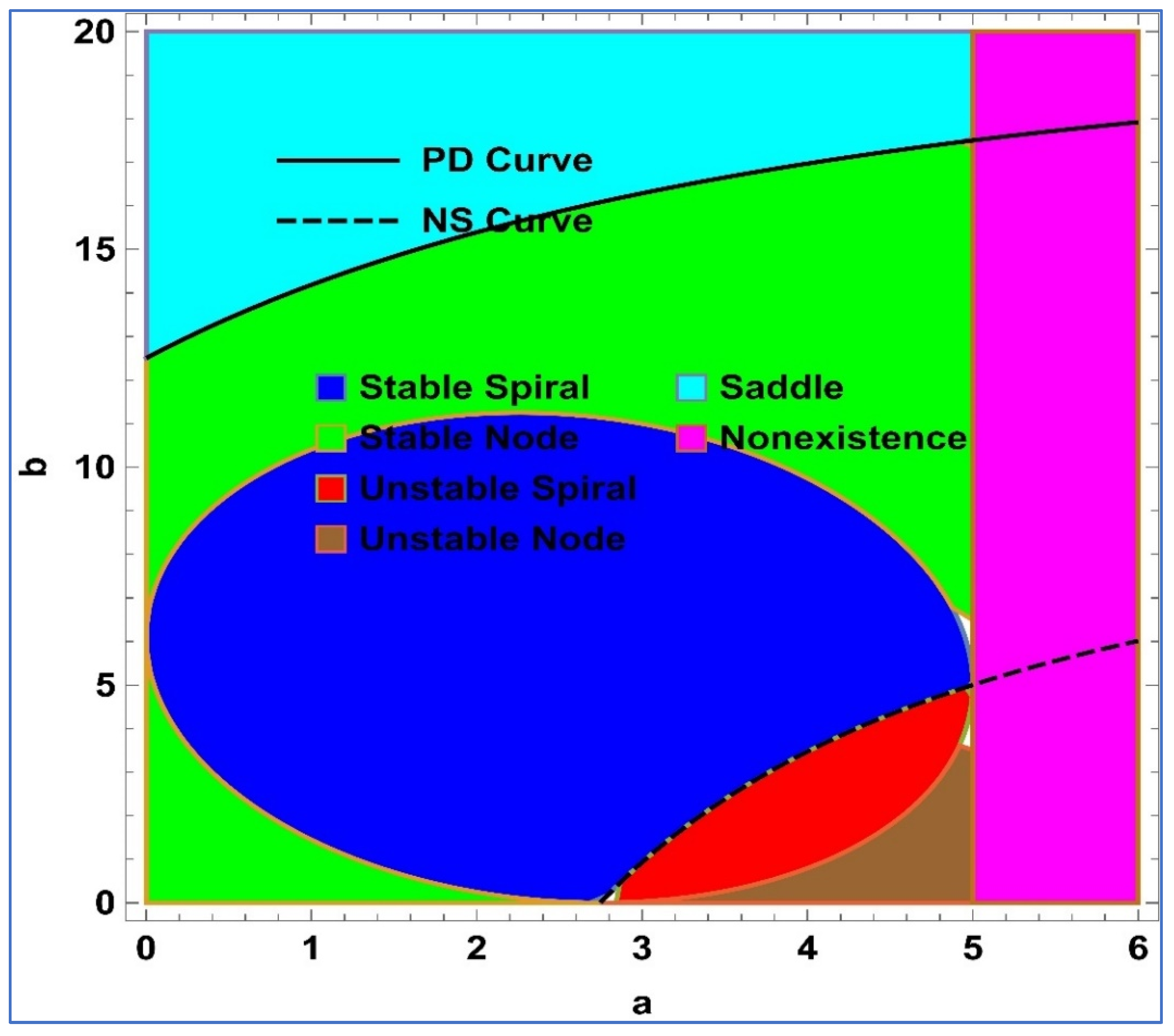
Lemma 1.

Assume that $0<c<1$ and $0<a<\frac{1}{1-c}$, then the following conditions hold true for the unique positive fixed point ($x^{*},y^{*}$) of system (4):

• ($x^{*},y^{*}$) is a stable spiral if $T^2-4D<0$, $1+T+D>0$, and $D<1$.
• ($x^{*},y^{*}$) is a stable node if ${ T}^2-4D>0$, $1+T+D>0$, and $D<1$.
• ($x^{*},y^{*}$) is an unstable spiral if $T^2-4D<0$, $1+T+D>0$, and $D>1$.
• ($x^{*},y^{*}$) is an unstable node if $T^2-4D>0$, $1+T+D>0$, and $D>1$.
• ($x^{*},y^{*}$) is a saddle point if $1+T+D<0$.

Furthermore, a visualization representation of Lemma 1 is given in Figure 1. On the other hand, PD and NS curves represent the period-doubling bifurcation curve and Neimark–Sacker bifurcation curve, respectively.

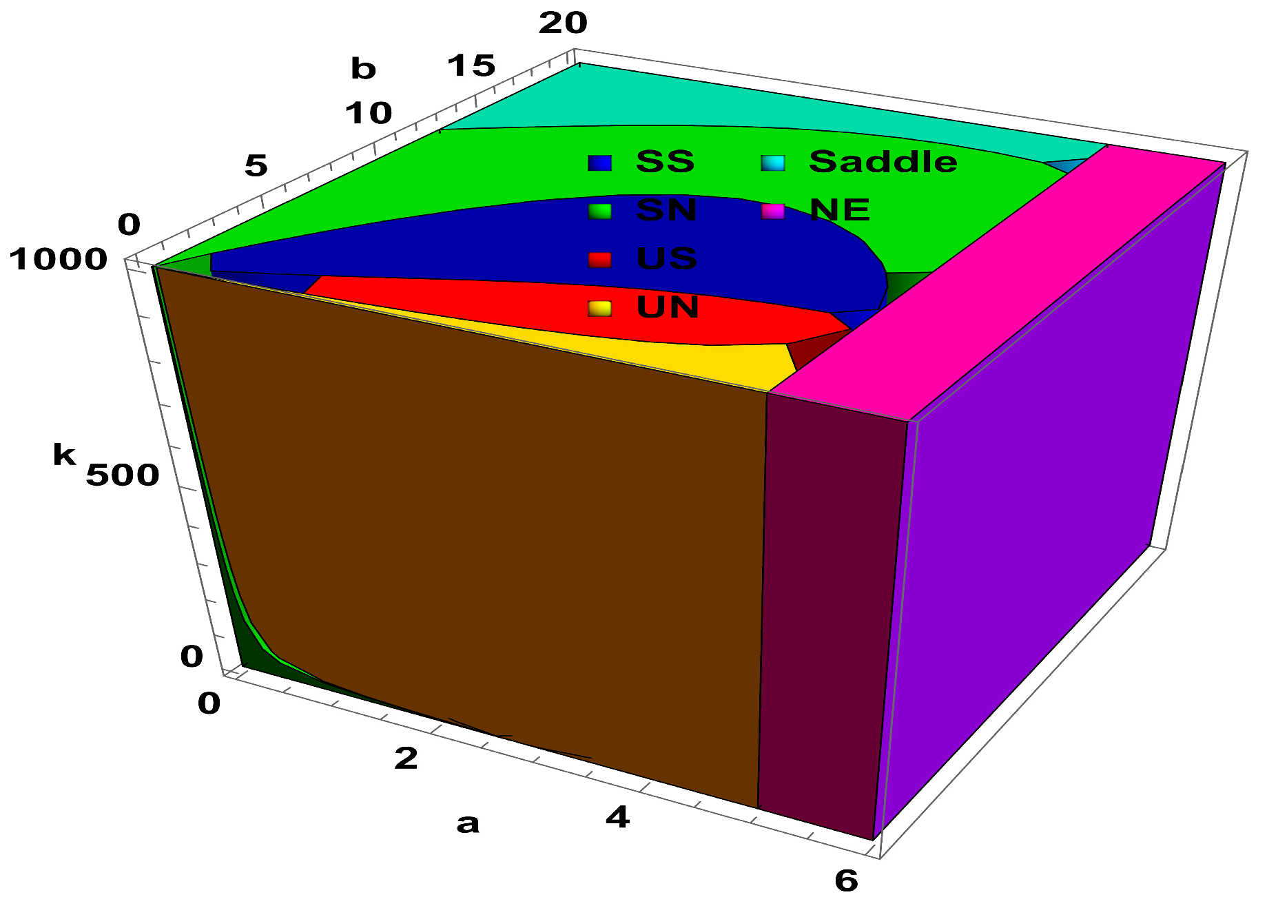
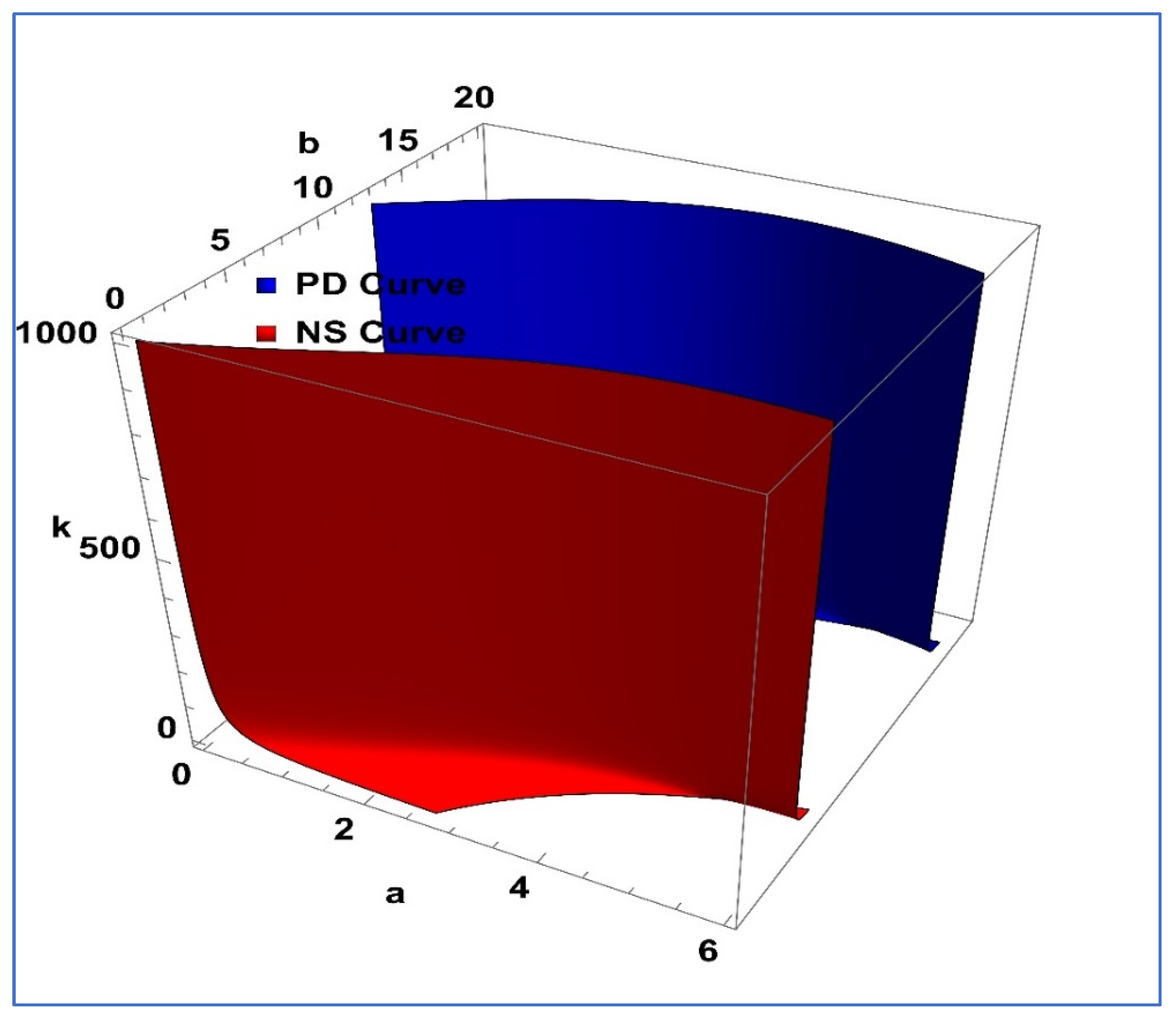
Secondly, dynamical behavior with respect to large variation in the level of fear $k\in [0, 1000]$ is taken into account, and corresponding results are depicted in Figure 2. The region in Figure 2 are stable spiral (SS), stable node (SN), unstable spiral (US), unstable node (UN), saddle, and nonexistence (NE). From Figure 2, it is easy to see that increasing the level of fear after a certain value has no significance of the dynamics of predator–prey interaction. Moreover, corresponding to Figure 2, the three-dimensional PD and NS curves are depicted in Figure 3.

3. Transcritical Bifurcation

In this section, emergence of transcritical bifurcation is investigated about predator-free fixed point (1, 0) of system (4). For this, $c$ is selected as bifurcation parameter. Then, from the calculation presented in the Section 2, it is easy to see that J(1, 0) has one eigenvalue ${\lambda }_2=1$ at $c=c_0:=1$.

Theorem 1.

Let $c\equiv c_0=1$, then system (4) undergoes transcritical bifurcation around its boundary fixed point $(1, 0)$ whenever the bifurcation parameter $c$ varies in small neighborhood of $c_0$.

Proof. 

Let $c=c_0$, and writing system (4) alternatively as follows:

$$\left(\genfrac{}{}{0pt}{}{x_1}{y_1}\right)\to \left( \genfrac{}{}{0pt}{}{x_1 e^{\left(\frac{1-x_1}{1+k y_1}-\frac{a y_1}{x_1+y_1}\right)}}{ y_1{e}^{ b \left(\frac{x_1}{x_1+y_1}-c_0\right)}}\right).$$

(7)

Taking $u=x_1-1$ and $y_1=v$ in system (7), one can obtain the following:

$$\left(\genfrac{}{}{0pt}{}{u}{v}\right)\to \left( \genfrac{}{}{0pt}{}{\left(u+1\right)e^{\left(\frac{-u}{1+k v}-\frac{a \left(u+1\right)}{u+1+v}\right)}-1}{ v e^{ b \left(\frac{u+1}{u+1+v}-c_0-\overline{c}\right)}}\right),$$

(8)

where $\left|\overline{c}\right|\ll 1$ is a small perturbation parameter and taken as bifurcation parameter. Then, from (8), it follows that:

$$\left(\begin{array}{c}u\\ v\end{array}\right)\to \left(\begin{array}{cc}0& -a\\ 0& 1\end{array}\right)\left(\begin{array}{c}u\\ v\end{array}\right)+\left(\begin{array}{c}\mathsf{\Phi } (u,v)\\ \mathsf{\Psi } (u,v,\overline{c})\end{array}\right),$$

(9)

where

$$\begin{array}{l}\mathsf{\Phi }\left(u,v\right)=-\frac{1}{2}{u}^2+\left(a+k\right)uv+\frac{1}{2}\left(2a+a^2\right)v^2+\frac{1}{3}{u}^3-\frac{a}{2}{u}^{2}v\\ -\left(a\left(2+a\right)+ak+k^2\right)u{v}^2-\frac{1}{6}a\left(6+a\left(6+a\right)\right)v^3\\ +O\left({\left(\left|u\right|+\left|v\right|\right)}^4\right),\end{array}$$

and

$$\begin{array}{c}\mathsf{\Psi }\left(u,v,\overline{c}\right)=-b{v}^2+bu{v}^2+\frac{1}{2}b\left(2+b\right)v^3-bv\overline{c}+b^2{v}^2\overline{c}+\frac{b^2}{2}v{\overline{c}}^2\\ +O\left({\left(\left|u\right|+\left|v\right|+\left|\overline{c}\right|\right)}^4\right).\end{array}$$

Next one can assume the following similarity transformation:

$$\left(\begin{array}{c}u\\ v\end{array}\right)=\left(\begin{array}{cc}-a& -a\\ 1& 0\end{array}\right) \left(\begin{array}{c}x\\ y\end{array}\right).$$

(10)

Using (10) in (9), we obtain the following system in canonical form:

$$\left(\begin{array}{c}x\\ y\end{array}\right)\to \left(\begin{array}{cc}0& 0\\ 0& 1\end{array}\right)\left(\begin{array}{c}x\\ y\end{array}\right)+\left(\begin{array}{c}{\mathsf{\Phi }}_1 (x,y,\overline{c})\\ {\mathsf{\Psi }}_1 (x,y,\overline{c})\end{array}\right),$$

(11)

where

$${\mathsf{\Phi }}_1\left(x,y,\overline{c}\right):=\mathsf{\Psi }\left(-a\left(x+y\right),x,\overline{c}\right),$$

and

$${\mathsf{\Psi }}_1\left(x,y,\overline{c}\right)=:-\frac{1}{a}\mathsf{\Phi }\left(-a\left(x+y\right),x\right)-\mathsf{\Psi }\left(-a\left(x+y\right),x,\overline{c}\right).$$

Next, suppose for the center manifold of system (11), we have

$$y_n=\zeta \left(x_n,\overline{c}\right)=:m_0{x_n}^2+m_1{x}_n\overline{c}+m_2{\overline{c}}^2+O\left({\left(\left|x_n\right|+\left|\overline{c}\right|\right)}^3\right),$$

where

$$m_0=a+b+k-1,m_1=b, \mathrm{and} m_2=0.$$

Then, system (11) is restricted to the following one-dimensional map:

$$\begin{array}{l}\mathsf{\Theta }:x\to x+{\mathsf{\Phi }}_1\left(x,\zeta \left(x,\overline{c}\right),\overline{c}\right)\\ =\frac{1}{2}x(2+b^2\left(\overline{c}+x\right)\left(\overline{c}+x-2a{x}^2\right)\\ -2b\left(\overline{c}+x+\left(a-1\right)x^2+a\left(a-1+k\right)x^3\right))\\ +O\left({\left(\left|x\right|+\left|\overline{c}\right|\right)}^5\right).\end{array}$$

Then, one can easily verify that:

$$\left|\begin{array}{c}\frac{\partial \mathsf{\Theta }(\mathrm{x},\overline{c})}{\partial x}\left(\mathrm{0,0}\right)=1; \frac{{\partial }^2\mathsf{\Theta }(\mathrm{x},\overline{c})}{\partial x^2}\left(\mathrm{0,0}\right)=-2 b\ne 0, \\ \frac{\partial \mathsf{\Theta }(\mathrm{x},\overline{c})}{\partial \overline{c}}\left(\mathrm{0,0}\right)=0; \frac{{\partial }^2\mathsf{\Theta }(\mathrm{x},\overline{c})}{\partial x\partial \overline{c}}\left(\mathrm{0,0}\right)=-b\ne 0. \end{array}\right.$$

Therefore, taking into account Winggins ([44], p. 507), all conditions for the emergence of transcritical bifurcation are satisfied. □

4. Period-Doubling Bifurcation

In the context of the occurrence of period-doubling bifurcation (PDB) about the interior equilibrium point of system $\left(4\right)$, we employ the concept of bifurcation theory, specifically the normal form and center manifold theorem. Moreover, Mathematica 13.2 software is used for all mathematical computation of this section.

Let $b$ represents the bifurcation parameter, and it is presupposed that:

$$b\equiv b_0=\frac{4k+2c\left(1+a-a{c}^2+\left(-2+a{\left(-1+c\right)}^2\right)k\right)}{\left(c-1\right)c\left(\left(-1+a\left(c-1\right)\right)c+\left(2+a\left(1+a\left(-1+c\right)\right)\left(c-1\right)\right)\left(c-1\right)k\right)}.$$

To define the period-doubling curve for the emergence of PDB in system (4) about its positive fixed point, the curve ${\mathit{S}}_{\mathit{P}\mathit{D}\mathit{B}}$ is defined as follows:

$${\mathit{S}}_{\mathit{P}\mathit{D}\mathit{B}}=\left\{\left(\alpha ,b,c,k\right)\in {\mathbb{R}}_{+}^4:b=b_0\right\}.$$

Let $\left(\alpha , b,c,k\right)\in {\mathit{S}}_{\mathit{P}\mathit{D}\mathit{B}}$, then system $\left(4\right)$ alternatively can be written by the following two-dimensional perturbed map:

$$\left(\genfrac{}{}{0pt}{}{U}{V}\right)\to \left( \genfrac{}{}{0pt}{}{U{e}^{\left(\frac{1-U}{1+kV}-\frac{\alpha V}{U_{+V}}\right)}}{V{e}^{\left(b_{0+}\overline{b}\right)\left(\frac{U}{U+V}-c\right)}}\right),$$

(12)

where $\overline{b}$ is very small perturbation in $b_0$. In order to apply bifurcation theory of normal forms, first we need a corresponding map for (12) whose fixed point must be shifted at origin. For this, we assume that $u=U-X$ and $v=V-Y$ then the map (12) is transformed as:

$$\left(\genfrac{}{}{0pt}{}{u}{v}\right)\to \left( \genfrac{}{}{0pt}{}{(u+X)e^{\left(\frac{1-(u+X)}{1+k(v+Y)}-\frac{\alpha (v+Y)}{{u+X}_{+v+Y}}\right)}}{(v+Y)e^{\left(b_{0+}\overline{b}\right)\left(\frac{u+X}{u+X+v+Y}-c\right)}}\right),$$

(13)

where

$$X:=\frac{c(1-a+ac)}{c+ak-2ack+a{c}^{2}k} \mathrm{and} Y:=\frac{(1-c)(1-a+ac)}{c+ak-2ack+a{c}^{2}k}.$$

The subsequent map can be derived by utilizing Taylor’s series to approximate the model described in section (9) around the point $\left(u,v,\overline{b}\right)=(0,0,0)$:

$$a_{11}=1+ac-a{c}^2+\frac{c+a\left(c-1\right)c}{c\left(-1+k\right)-k},a_{12}=\frac{ac(c^2-(c-1\left)\right(1+a(c-1)+c\left)k\right)}{c(-1+k)-k},$$

$$\left(\genfrac{}{}{0pt}{}{u}{v}\right)\to \left(\begin{array}{cc}{a}_{11}& a_{12}\\ {\mathrm{b}}_0{(c-1)}^2& 1+{\mathrm{b}}_0(c-1)c\end{array}\right)\left(\genfrac{}{}{0pt}{}{u}{v}\right)+\left(\genfrac{}{}{0pt}{}{f_1(u, v)}{g_1(u, v,\overline{b})}\right),$$

(14)

where

$$\begin{array}{ll}{f}_1\left(u,v\right)={\mathrm{a}}_{200}{u}^2& +{\mathrm{a}}_{110}uv+{\mathrm{a}}_{020}{v}^2+{\mathrm{a}}_{300}{u}^3+{\mathrm{a}}_{210}{u}^{2}v+{\mathrm{a}}_{120}u{v}^2+{\mathrm{a}}_{030}{v}^3\\ & +O\left({\left(\left|u\right|+\left|v\right|\right)}^4\right),\end{array}$$

$$\begin{array}{ll}{g}_1\left(u,v,\overline{b}\right)=& b_{200}{u}^2+{\mathrm{b}}_{110}uv+{\mathrm{b}}_{020}{v}^2+{\mathrm{b}}_{300}{u}^3+{\mathrm{b}}_{120}{u}^{2}v+{\mathrm{b}}_{030}{v}^3+{\mathrm{b}}_{101}u\overline{b}\\ & +b_{011}v\overline{b}+{\mathrm{b}}_{111}uv\overline{b}+{\mathrm{b}}_{201}{u}^2\overline{b}+{\mathrm{b}}_{021}{v}^2\overline{b}+{\mathrm{b}}_{102}u{\overline{b}}^2\\ & +{\mathrm{b}}_{012}v{\overline{b}}^2+b_{003}{\overline{b}}^3+O\left({\left(\left|u\right|+\left|v\right|+\left|\overline{b}\right|\right)}^4\right).\end{array}$$

Moreover, $a_{200},a_{110},a_{020},a_{300},a_{210},a_{120},a_{030},b_{200},b_{110},b_{020},b_{300},b_{120},b_{300},b_{101},b_{011},b_{111},b_{201},b_{021},b_{102},b_{012},b_{003}$ are given as follows:

$$\begin{array}{ll}{\mathrm{a}}_{200}=& \frac{1}{2{\left(X+Y\right)}^4{\left(1+kY\right)}^2}(X^5-2X^4\left(1+\left(-2+k\right)Y\right)\\ & +2Y^3\left(1+kY\right)\left(a-Y+akY\right)\\ & -4X^2{Y}^2\left(3+a+\left(-1+\left(3+a\right)k\right)Y\right)\\ & -2X^{3}Y\left(4+a+\left(-3+\left(4+a\right)k\right)Y\right)\\ & +X{Y}^2(Y\left(-8+Y-8kY\right)+2a\left(1+\left(-1+k\right)Y\right)\left(1+kY\right)\\ & +{\left(a+akY\right)}^2\left)\right),\end{array}$$

$$\begin{array}{ll}{\mathrm{a}}_{110}=& \frac{1}{{\left(X+Y\right)}^4{\left(1+kY\right)}^3}(-a^2{X}^{2}Y{\left(1+kY\right)}^3\\ & -k{\left(X+Y\right)}^4\left(1+kY+X\left(-3+X-2kY\right)\right)\\ & +aX\left(X+Y\right)\left(1+kY\right)(X^2\left(1+2kY\right)-Y\left(2+kY\right)\left(1+2kY\right)\\ & +XY\left(1-k+2kY\right)\left)\right),\end{array}$$

$$\begin{array}{ll}{\mathrm{a}}_{020}=& \frac{1}{2{\left(X+Y\right)}^4{\left(1+kY\right)}^4}X(k^2\left(X-1\right){\left(X+Y\right)}^4\left(-3+X-2kY\right)\\ & +a^2{X}^2{\left(1+kY\right)}^4\\ & -2aX\left(X+Y\right){\left(1+kY\right)}^2(-1\\ & +k\left(X^2+X\left(Y-1\right)-Y\left(3+kY\right)\right)\left)\right),\end{array}$$

$$\begin{array}{ll}{\mathrm{a}}_{300}=& \frac{1}{6{\left(X+Y\right)}^6{\left(1+kY\right)}^3}(-X^7+3X^6\left(1+\left(-2+k\right)Y\right)\\ & +3X^{5}Y\left(6+a+\left(-5+\left(6+a\right)k\right)Y\right)\\ & +X^4{Y}^2\left(45+5\left(-4+9k\right)Y+12a\left(1+kY\right)\right)\\ & -3X^3{Y}^2(5Y\left(-4+Y-4kY\right)+2a\left(1+\left(-3+k\right)Y\right)\left(1+kY\right)\\ & +{\left(a+akY\right)}^2)\\ & +3Y^4\left(1+kY\right)\left(Y^2-2a\left(1+kY\right)\left(1+Y+kY\right)+{\left(a+akY\right)}^2\right)\\ & -3X^2{Y}^2(Y^2\left(-15+\left(2-15k\right)Y\right)\\ & +{\left(a+akY\right)}^2\left(1+\left(2+k\right)Y\right)\\ & +2a\left(1+kY\right)\left(1+Y\left(3+2k+\left(-2+k\left(3+k\right)\right)Y\right)\right))\\ & +X{Y}^3(-3Y{\left(a+akY\right)}^2+{\left(a+akY\right)}^3\\ & +Y^2\left(18+\left(-1+18k\right)Y\right)\\ & -3a\left(1+kY\right)\left(4+Y\left(6-Y+2k\left(4+\left(3+2k\right)Y\right)\right)\right)\left)\right),\end{array}$$

$$\begin{array}{ll}{\mathrm{a}}_{210}=& \frac{1}{2{\left(X+Y\right)}^6{\left(1+kY\right)}^4}(-a^3{X}^2{Y}^2{\left(1+kY\right)}^4\\ & +k{\left(X+Y\right)}^6\left(X^2+2\left(1+kY\right)\left(2+kY\right)-X\left(5+4kY\right)\right)\\ & +XY\left(X+Y\right){\left(a+akY\right)}^2(X^2\left(2+3kY\right)-Y\left(4+kY\left(9+4kY\right)\right)\\ & +X\left(2+Y\left(2+3k+k\left(3+2k\right)Y\right)\right))\\ & -a{\left(X+Y\right)}^2\left(1+kY\right)(X^4\left(1+3kY\right)\\ & -2X^{3}Y\left(-1+2k+\left(-3+k\right)kY\right)\\ & +X^{2}Y\left(-4+Y+kY\left(-18+3Y-10kY\right)\right)\\ & +2Y^2\left(1+kY\right)\left(1+kY\left(3+kY\right)\right)\\ & -2XY\left(2+Y\left(2+k\left(5+Y\left(7+5k+2k\left(2+k\right)Y\right)\right)\right)\right)\left)\right),\end{array}$$

$$\begin{array}{ll}{\mathrm{a}}_{120}=& \frac{1}{2{\left(X+Y\right)}^6{\left(1+kY\right)}^5}(a^3{X}^{3}Y{\left(1+kY\right)}^5\\ & -k^2{\left(X+Y\right)}^6(-3+X\left(11+\left(X-7\right)X\right)-5kY\\ & +k\left(14-5X\right)XY+2k^2\left(2X-1\right)Y^2)\\ & -a^2{X}^2\left(X+Y\right){\left(1+kY\right)}^3(X^2\left(1+3kY\right)\\ & +X\left(1+Y+k\left(3+k\right)Y^2\right)-Y\left(5+kY\left(12+5kY\right)\right))\\ & +aX{\left(X+Y\right)}^2\left(1+kY\right)(k{X}^4\left(2+3kY\right)\\ & -2k{X}^3\left(2+Y\left(-2+5k+k\left(-3+2k\right)Y\right)\right)\\ & -2X\left(1+Y+kY\left(2+Y\left(1+kY\right)\left(7-k+k\left(5+k\right)Y\right)\right)\right)\\ & +X^2\left(-2+kY\left(2\left(Y-9\right)+k\left(3+Y\left(2k+3Y-14kY-34\right)\right)\right)\right)\\ & +Y\left(4+kY\left(20+kY\left(35+2kY\left(11+2kY\right)\right)\right)\right)\left)\right),\end{array}$$

$$\begin{array}{ll}{\mathrm{a}}_{030}=& \frac{1}{6{\left(X+Y\right)}^6{\left(1+kY\right)}^6}X(-a^3{X}^3{\left(1+kY\right)}^6\\ & +k^3\left(-1+X\right){\left(X+Y\right)}^6(13+X^2+6kY\left(3+kY\right)\\ & -2X\left(4+3kY\right))\\ & -3aX{\left(X+Y\right)}^2{\left(1+kY\right)}^2(2\\ & +k(\left(-1+X\right)X\left(-2+k\left(-3+X\right)X\right)\\ & -2\left(-5+X+k\left(-1+X\right)X\left(5+\left(-1+k\right)X\right)\right)Y\\ & +k\left(19+X\left(-8-6k\left(-1+X\right)+X\right)\right)Y^2-4k^2\left(-3+X\right)Y^3\\ & +2k^3{Y}^4\left)\right)\\ & +3a^2{X}^2\left(X+Y\right){\left(1+kY\right)}^4(-2\\ & +k\left(X^2+X\left(-1+Y\right)-Y\left(5+2kY\right)\right)\left)\right),\end{array}$$

$$\begin{array}{l}{b}_{200}=\frac{{\mathrm{b}}_0{Y}^2(-2X+({\mathrm{b}}_0-2\left)Y\right)}{2{(X+Y)}^4},b_{110}=\frac{{\mathrm{b}}_{0}XY(2X-({\mathrm{b}}_0-2\left)Y\right)}{{(X+Y)}^4},{\mathrm{b}}_{020}\\ =\frac{{\mathrm{b}}_0{X}^2(-2X+({\mathrm{b}}_0-2\left)Y\right)}{2{(X+Y)}^4},b_{300}\\ =\frac{{\mathrm{b}}_0(6X^2-6({\mathrm{b}}_0-2)XY+(6+({\mathrm{b}}_0-6)\mathrm{b}0\left)Y^2\right)}{6{(X+Y)}^6}{,\mathrm{b}}_{120}\\ =-\frac{{\mathrm{b}}_{0}Y(4X^3+(6-5{\mathrm{b}}_0)X^{2}Y+({\mathrm{b}}_0-4)\mathrm{b}0X{Y}^2+({\mathrm{b}}_0-2\left)Y^3\right)}{2{(X+Y)}^6}{,b}_{030}\\ =\frac{{\mathrm{b}}_0{X}^2(3\left(2+{\mathrm{b}}_0\right)X^2-\left({{\mathrm{b}}_0}^2-12\right)XY-3({\mathrm{b}}_0-2\left)Y^2\right)}{6{(X+Y)}^6}\end{array}$$

$$\begin{array}{ll}{\mathrm{b}}_{101}=& \frac{1}{6{\left(X+Y\right)}^9}X(6\left(-2-{\mathrm{b}}_0\left(4+{\mathrm{b}}_0\right)+{\mathrm{b}}_0\left(2+{\mathrm{b}}_0\right)c\right)X^5\\ & -6\left(6+{\mathrm{b}}_0\left(2-6c+{\mathrm{b}}_0\left(-5+{\mathrm{b}}_0\left(-1+c\right)+c\right)\right)\right)X^{4}Y\\ & +(-24\\ & +{\mathrm{b}}_0(24\left(4+c\right)\\ & +{\mathrm{b}}_0\left(54-{\mathrm{b}}_0\left(4+{\mathrm{b}}_0\right)-48c+\left(-6+{\mathrm{b}}_0\right){\mathrm{b}}_{0}c\right)\left)\right)X^3{Y}^2\\ & +(24-2{\mathrm{b}}_0\left(-60+{\mathrm{b}}_0\left(3+5{\mathrm{b}}_0\right)\right)\\ & +{\mathrm{b}}_0\left(-24+{\mathrm{b}}_0\left(-48+\mathrm{b}0\left(6+{\mathrm{b}}_0\right)\right)\right)c)X^2{Y}^3\\ & +6\left(6+{\mathrm{b}}_0\left(4-6c+{\mathrm{b}}_0\left(-4+\left(-1+{\mathrm{b}}_0\right)c\right)\right)\right)X{Y}^4\\ & +6\left(2-2{\mathrm{b}}_0+\left(-2+{\mathrm{b}}_0\right){\mathrm{b}}_{0}c\right)Y^5),\end{array}$$

$$\begin{array}{l}{b}_{011}=\frac{(-((c-1)X^3)+(1+{\mathrm{b}}_0(c-1)-3c)X^{2}Y+({\mathrm{b}}_0-3)cX{Y}^2-c{Y}^3)}{{(X+Y)}^3},b_{111}\\ =-\frac{XY\left(2\left(-1+b_0\left(c-1\right)\right)x^2+\left({{\mathrm{b}}^2}_0-4-\left(b_0-4\right)b_{0}c\right)XY+\left({\mathrm{b}}_0-2\left(2-\left({\mathrm{b}}_0-2\right)c\right)\right)y^2\right)}{{\left(X+Y\right)}^5},b_{201}\\ =-\frac{Y^2\left(2\left(1+b_0-b_{0}c\right)X^2+\left(4+{{\mathrm{b}}^2}_0\left(c-1\right)-4b_{0}c\right)XY+\left(2-2b_0+\left(b_0-2\right)b_{0}c\right)Y^2\right)}{2{\left(X+Y\right)}^5},b_{021}\\ =\frac{X^2\left(2\left(-1+b_0\left(c-1\right)\right)X^2+\left(-4+{{\mathrm{b}}^2}_0-\left(b_0-4\right)b_{0}c\right)XY+\left(-2+b_0\left(2-\left(b_0-2\right)c\right)\right)Y^2\right)}{2{\left(X+Y\right)}^5},{\mathrm{b}}_{102}\\ =\frac{Y^2\left(\left(c-1\right)X+cY\right)\left(\left(-2+{\mathrm{b}}_0\left(c-1\right)\right)X+\left({\mathrm{b}}_{0}c-2\right)Y\right)}{2{\left(X+Y\right)}^4},b_{012}\\ =\frac{\left(\left(c-1\right)X+cY\right)\left(\left(c-1+\right)X^3+\left(b_0+3c-b_{0}c\right)X^{2}Y+\left(1-\left(b_0-3\right)c\right)X{Y}^2+c{Y}^3\right)}{2}{\left(X+Y\right)}^4,b_{003}\\ =-\frac{Y{\left(\left(-1+c\right)X+cY\right)}^3}{6{\left(X+Y\right)}^3}.\end{array}$$

Suppose that $(a, b, c, k)\in S_{PDB}$, the eigenvalues of Jacobian matrix

$$B=\left(\begin{array}{cc}{a}_{11}& {\mathrm{a}}_{12}\\ {\mathrm{b}}_0{(c-1)}^2& 1+{\mathrm{b}}_0(c-1)c\end{array}\right),$$

are given by ${\lambda }_1=-1$ and

$$\begin{array}{ll}{\lambda }_2=& \left(\right((c-1)\left(a\right(-1+c\left)c^2\right(1+a+ac)+(-1+a(c-1)\left)c\right(1+a(c-1)(c\\ & +a(c^2-1)\left)\right)k-(c-1)(-2+a(1+a(c-1)\left)\right(c-1\left)\right(-3\\ & +a(c-1)c\left)\right)k^2\left)\right))⁄(\left(c^2\right(1+a-ac)-(3+a^2{(c-1)}^2\left)\right(c\\ & -1)ck+(2+a(1+a(c-1\left)\right)(c-1)\left){(c-1)}^2{k}^2\right))\end{array}$$

Additionally, let us presume that ${\lambda }_2\ne \pm 1$, and let us examine the subsequent transformation:

$$\left(\begin{array}{c}U\\ V\end{array}\right)=T\left(\begin{array}{c}x\\ y\end{array}\right),$$

(15)

where T $=\left(\begin{array}{cc}{a}_{12}& a_{12}\\ -1-a_{11}& {\lambda }_2-a_{11}\end{array}\right)$, and $T^{-1}=\left(\begin{array}{cc}\frac{-{\mathrm{a}}_{11}+{\mathsf{\lambda }}_2}{{\mathrm{a}}_{12}+{\mathrm{a}}_{12}{\mathsf{\lambda }}_2}& -\frac{1}{1+{\mathsf{\lambda }}_2}\\ \frac{1+\mathrm{a}11}{{\mathrm{a}}_{12}+{\mathrm{a}}_{12}{\mathsf{\lambda }}_2}& \frac{1}{1+{\mathsf{\lambda }}_2}\end{array}\right)$.

From $\left(14\right)$ and $\left(15\right)$, we obtain

$$\left(\begin{array}{c}x\\ y\end{array}\right)\to \left(\begin{array}{cc}-1& 0\\ 0& {\lambda }_2\end{array}\right)\left(\begin{array}{c}x\\ y\end{array}\right)+\left(\begin{array}{c}{f}_2(x,y,\overline{b}\\ g_2(x,y,\overline{b})\end{array}\right),$$

(16)

where

$$\begin{gathered} f_2\left(x,y,\overline{b}\right)=-\frac{{\mathrm{g}}_1\left[{\mathrm{a}}_{12}\left(x+y\right),-\left(\left(1+{\mathrm{a}}_{11}\right)x\right)+y\left(-{\mathrm{a}}_{11}+{\mathsf{\lambda }}_2\right),b\right]}{1+{\mathsf{\lambda }}_2}+ \\ \frac{f_1\left[{\mathrm{a}}_{12}\left(x+y\right),-\left(\left(1+{\mathrm{a}}_{11}\right)x\right)+y\left(-{\mathrm{a}}_{11}+{\mathsf{\lambda }}_2\right)\right]\left(-{\mathrm{a}}_{11}+{\mathsf{\lambda }}_2\right)}{{\mathrm{a}}_{12}+{\mathrm{a}}_{12}{\mathsf{\lambda }}_2}, \end{gathered}$$

$$\begin{gathered} g_2\left(x,y,\overline{b}\right)=\frac{\left(1+{\mathrm{a}}_{11}\right){\mathrm{f}}_1\left[{\mathrm{a}}_{12}\left(x+y\right),-\left(\left(1+{\mathrm{a}}_{11}\right)x\right)+y\left(-{\mathrm{a}}_{11}+{\mathsf{\lambda }}_2\right)\right]}{{\mathrm{a}}_{12}+{\mathrm{a}}_{12}{\mathsf{\lambda }}_2}+ \\ \frac{{\mathrm{g}}_1\left[{\mathrm{a}}_{12}\left(x+y\right),-\left(\left(1+{\mathrm{a}}_{11}\right)x\right)+y\left(-{\mathrm{a}}_{11}+{\mathsf{\lambda }}_2\right),b\right]}{1+{\mathsf{\lambda }}_2}. \end{gathered}$$

By applying center manifold theory [45], one can conduct a stability analysis of the equilibrium point at $(x, y)=(0,0)$ in the vicinity of $\overline{ b}=0$. This analysis entails investigating a set of simplified equations characterized by a single parameter. The primary focus is on a central manifold identified as $W^C(0,0,0)$. This center manifold can be defined as follows:

$$W^C\left(0,0,0\right)=\left\{\left(x,y,\overline{b}\right)\in R^3:y=k_0{x}^2+k_{1}x\overline{b}+k_2{\overline{b}}^2+O\left({\left(\left|u\right|+\left|\overline{b}\right|\right)}^3\right)\right\},$$

where

$$k_0=\frac{-a_{020}{\left(1+{\mathrm{a}}_{11}\right)}^3+\left(1+{\mathrm{a}}_{11}\right){\mathrm{a}}_{12}\left(\left(1+{\mathrm{a}}_{11}\right){\mathrm{a}}_{110}-\left(1+{\mathrm{a}}_{11}\right)b_{020}+{\mathrm{a}}_{12}\left(b_{110}-a_{200}\right)\right)-{{\mathrm{a}}_{12}}^3{b}_{200}}{a_{12}\left({{\lambda }^2}_2-1\right)},$$

$$k_1=\frac{b_{011}+a_{11}{b}_{011}-a_{12}{b}_{101}}{{(1+{\lambda }_2)}^2};k_2=0.$$

In a significance, the restriction for system (3.1.6) in accordance with its center manifold ${\mathrm{W}}^C\left(0,0,0\right)$ can be presented as follows:

$$\mathbf{F}:x\to -x+{\mathrm{h}}_1{x}^2+{\mathrm{h}}_{2}x\overline{b}+{\mathrm{h}}_3{x}^2\overline{b}+{\mathrm{h}}_{4}x{\overline{b}}^2+{\mathrm{h}}_5{x}^3+O\left({\left(\left|x\right|+\left|\overline{b}\right|\right)}^4\right),$$

$$\begin{array}{ll}{\mathrm{h}}_1=& -\frac{1}{{\mathrm{a}}_{12}\left(1+{\mathsf{\lambda }}_2\right)}({\mathrm{a}}_{020}{\left(1+{\mathrm{a}}_{11}\right)}^2\left({\mathrm{a}}_{11}-{\mathsf{\lambda }}_2\right)\\ & +{\mathrm{a}}_{12}({\mathrm{b}}_{020}+{{\mathrm{a}}_{11}}^2\left({\mathrm{b}}_{020}-{\mathrm{a}}_{110}\right)+{{\mathrm{a}}_{12}}^2{\mathrm{b}}_{200}\\ & +{\mathrm{a}}_{11}\left({\mathrm{a}}_{12}{\mathrm{a}}_{200}+2{\mathrm{b}}_{020}-{\mathrm{a}}_{12}{\mathrm{b}}_{110}+{\mathrm{a}}_{110}\left({\mathsf{\lambda }}_{2}1\right)\right)+{\mathrm{a}}_{110}{\mathsf{\lambda }}_2\\ & -{\mathrm{a}}_{12}\left({\mathrm{b}}_{110}+{\mathrm{a}}_{200}{\mathsf{\lambda }}_2\right)\left)\right),\end{array}$$

$${\mathrm{h}}_2=\frac{{\mathrm{b}}_{011}+{\mathrm{a}}_{11}{\mathrm{b}}_{011}-{\mathrm{a}}_{12}{\mathrm{b}}_{101}}{1+{\mathsf{\lambda }}_2},$$

$$\begin{array}{ll}{\mathrm{h}}_3=& \frac{1}{{\mathrm{a}}_{12}\left(1+{\mathsf{\lambda }}_2\right)}(-{\left(1+{\mathrm{a}}_{11}\right)}^2{\mathrm{a}}_{12}{\mathrm{b}}_{021}-{{\mathrm{a}}_{12}}^3({\mathrm{b}}_{201}+2{\mathrm{b}}_{200}{\mathrm{c}}_1)+{\mathrm{a}}_{12}{b}_{001}{\mathrm{c}}_0\\ & -2(1+{\mathrm{a}}_{11}){\mathrm{b}}_{020}{\mathrm{c}}_1+{\mathrm{a}}_{110}{\mathrm{c}}_1(1+2{\mathrm{a}}_{11}-{\mathsf{\lambda }}_2)\left)\right({\mathrm{a}}_{11}-{\mathsf{\lambda }}_2)\\ & -2{\mathrm{a}}_{020}(1+{\mathrm{a}}_{11}){\mathrm{c}}_1{\left({\mathrm{a}}_{11}-{\mathsf{\lambda }}_2\right)}^2+{{\mathrm{a}}_{12}}^2\left(\right(1+{\mathrm{a}}_{11}){\mathrm{b}}_{111}-{\mathrm{b}}_{101}{\mathrm{c}}_0\\ & +{\mathrm{c}}_1({\mathrm{b}}_{110}+-2{\mathrm{a}}_{11}{\mathrm{a}}_{200}+2{\mathrm{a}}_{11}{\mathrm{b}}_{110}+2{\mathrm{a}}_{200}{\mathsf{\lambda }}_2-{\mathrm{b}}_{110}{\mathsf{\lambda }}_2)\left)\right),\end{array}$$

$${\mathrm{h}}_4=\frac{(1+{\mathrm{a}}_{11}){\mathrm{b}}_{012}-{\mathrm{a}}_{12}({\mathrm{b}}_{102}+{\mathrm{b}}_{101}{\mathrm{c}}_1)+{\mathrm{b}}_{011}{\mathrm{c}}_1({\mathrm{a}}_{11}-{\mathsf{\lambda }}_2)}{1+{\mathsf{\lambda }}_2},$$

$$\begin{array}{ll}{\mathrm{h}}_5=& \frac{1}{{\mathrm{a}}_{12}\left(1+{\mathsf{\lambda }}_2\right)}({{\mathrm{a}}_{11}}^3\left({\mathrm{a}}_{12}\left({\mathrm{b}}_{300}-{\mathrm{a}}_{120}\right)-2{\mathrm{a}}_{020}{\mathrm{c}}_0\right)\\ & +{\mathrm{a}}_{12}({\mathrm{b}}_{300}\\ & -{\mathrm{a}}_{12}\left({\mathrm{b}}_{120}-{\mathrm{b}}_{110}{\mathrm{c}}_0+{\mathrm{a}}_{12}\left({\mathrm{a}}_{12}{\mathrm{b}}_{300}-{\mathrm{b}}_{210}+2{\mathrm{b}}_{200}{\mathrm{c}}_0\right)\right))\\ & +{\mathrm{a}}_{030}{\left(1+{\mathrm{a}}_{11}\right)}^3\left({\mathrm{a}}_{11}-{\mathsf{\lambda }}_2\right)\\ & +{\mathrm{a}}_{12}({\mathrm{a}}_{120}+{\mathrm{a}}_{12}\left({\mathrm{a}}_{12}{\mathrm{a}}_{300}-{\mathrm{a}}_{210}\right)\\ & -\left({\mathrm{a}}_{110}-2\left({\mathrm{a}}_{12}{\mathrm{a}}_{200}+{\mathrm{b}}_{020}\right)+{\mathrm{a}}_{12}{\mathrm{b}}_{110}\right){\mathrm{c}}_0){\mathsf{\lambda }}_2\\ & +\left(-2{\mathrm{a}}_{020}+{\mathrm{a}}_{110}{\mathrm{a}}_{12}\right){\mathrm{c}}_0{{\mathsf{\lambda }}^2}_0\\ & +{{\mathrm{a}}_{11}}^2({{\mathrm{a}}_{12}}^2\left({\mathrm{a}}_{210}-{\mathrm{b}}_{120}\right)\\ & +{\mathrm{a}}_{12}\left(3{\mathrm{b}}_{300}+2{\mathrm{a}}_{110}{\mathrm{c}}_0-2{\mathrm{b}}_{020}{\mathrm{c}}_0+{\mathrm{a}}_{120}\left({\mathsf{\lambda }}_2-2\right)\right)\\ & +2{\mathrm{a}}_{020}{\mathrm{c}}_0\left(2{\mathsf{\lambda }}_2-1\right))\\ & +{\mathrm{a}}_{11}({{\mathrm{a}}_{12}}^3\left({\mathrm{b}}_{210}-{\mathrm{a}}_{300}\right)-2{\mathrm{a}}_{020}{\mathrm{c}}_0\left({\mathsf{\lambda }}_2-2\right){\mathsf{\lambda }}_2\\ & +{{\mathrm{a}}_{12}}^2\left({\mathrm{a}}_{210}-2\left({\mathrm{b}}_{120}+{\mathrm{a}}_{200}{\mathrm{c}}_0-{\mathrm{b}}_{110}{\mathrm{c}}_0\right)-{\mathrm{a}}_{210}{\mathsf{\lambda }}_2\right)\\ & +{\mathrm{a}}_{12}(3{\mathrm{b}}_{300}+{\mathrm{a}}_{120}\left(2{\mathsf{\lambda }}_2-1\right)\\ & +{\mathrm{c}}_0\left({\mathrm{a}}_{110}+2{\mathrm{b}}_{020}\left({\mathsf{\lambda }}_2-1\right)-3{\mathrm{a}}_{110}{\mathsf{\lambda }}_2\right)\left)\right)),\end{array}$$

Moreover, the representation of two non-zero values, denoted as $l_1$ and$l_2$, is demonstrated as follows:

$$l_1:={\left(\frac{{\partial }^2\mathbf{F}}{\partial u\partial \overline{b}}+\frac{1}{2}\frac{\partial \mathbf{F}}{\partial \overline{b}}\frac{{\partial }^2\mathbf{F}}{\partial x^2}\right)}_{\left(\mathrm{0,0}\right)}={\mathrm{h}}_2,$$

and

$$l_2:={\left(\frac{1}{6}\frac{{\partial }^3\mathbf{F}}{\partial x^3}+{\left(\frac{1}{2}\frac{{\partial }^2\mathbf{F}}{\partial x^2}\right)}^2\right)}_{(0,0)}={h_1}^2+h_5.$$

Taking into consideration the aforementioned calculation, the subsequent theorem provides the parametric circumstances that determine the presence and trajectory of a Positive Definite Boundary (PDB) for system (4) at its non-negative equilibrium point.

Theorem 2.

If both $l_1$ and $l_2$ are non-zero, system $\left(4\right)$ experiences a period-doubling bifurcation at its stable equilibrium point ($x^{*},y^{*})$ when the parameter $b$ changes within a small neighborhood around $b_0$. Moreover, when $l_2>0$, the period-two orbits originating from ${(x}^{*},y^{*})$ are stable, and if ${ l}_2<0$, these orbits become unstable.

5. Neimark–Sacker Bifurcation

This portion will predominantly center on examining the potential occurrence of a Neimark–Sacker bifurcation (NB) in proximity to the positive equilibrium point of model $\left(4\right)$. As we endeavor to accomplish this objective, it is important to consider that the solutions of Equation $\left(6\right)$ are anticipated to manifest as pairs of complex conjugates with a magnitude of one. Furthermore, we introduce the parameter $b$ as the bifurcation parameter and define the set $S_{NS}$ as described below:

$$S_{NS}=\left\{\left(a,b,c,k\right)\in {\mathbb{R}}_{+}^4:b=b_1,\left|A\right|<2\right\},$$

where

$$A=2-\left(a-b_1\right)\left(c-1\right)c+\frac{c+a\left(c-1\right)c}{c\left(k-1\right)-k},$$

and

$$b_1:=\frac{a-1-a{c}^2+a{(c-1)}^{2}k}{{(c-1)}^2(ac+k+a(1+a(c-1)\left)\right(c-1\left)k\right)}$$

Assume that $\left(\alpha ,b,c,k \right)\in S_{NS}$, then model (4) can be written in the subsequent mapping:

$$\left(\genfrac{}{}{0pt}{}{x}{y}\right)\to \left(\genfrac{}{}{0pt}{}{x{e}^{\left(\frac{1-x}{1+ky}-\frac{\alpha y}{x_{+v}}\right)}}{y{e}^{\left({b_1}_{+}\tilde{b}\right)\left(\frac{x}{x+y}-c\right)}}\right),$$

(17)

here $\tilde{b}$ denotes a slight perturbation in $b_1$. For further analysis, the following translations are considered $w=x-X$ and$z=y-Y$, then it follows from (17) that:

$$\left(\genfrac{}{}{0pt}{}{w}{z}\right)\to \left(\genfrac{}{}{0pt}{}{(w+X)e^{\left(\frac{1-(w+X)}{1+k(z+Y)}-\frac{\alpha (z+Y)}{{(w+X)}_{+(z+Y)}}\right)}}{(z+Y)e^{\left({b_1}_{+}\tilde{b}\right)\left(\frac{(w+X)}{(w+X)+(z+Y)}-c\right)}}\right).$$

(18)

Enlargement of Taylor’s series around $\left(w,z\right)=(0,0)$ results as follows:

$$\left(\genfrac{}{}{0pt}{}{w}{z}\right)\to \left(\begin{array}{cc}{d}_{11}& d_{12}\\ d_{13}& d_{14}\end{array}\right)\left(\genfrac{}{}{0pt}{}{w}{z}\right)+\left(\genfrac{}{}{0pt}{}{\mathsf{\phi }(w,z)}{\psi (w,z,}\right),$$

(19)

where

$$\begin{array}{ll}\mathsf{\varphi }\left(w,z\right)=& m_{12}{w}^2+m_{13}wz+m_{14}{z}^2+m_{15}{w}^3+m_{16}{w}^{2}z+m_{17}w{z}^2+m_{18}{z}^3\\ & +O\left({\left(\left|w\right|+\left|z\right|\right)}^4\right),\end{array}$$

$$\psi \left(w,z\right)=l_{22}{u}^2+l_{23}wz+l_{24}{z}^2+l_{24}{w}^3+l_{25}{w}^{2}z+l_{26}{z}^3+O\left({\left(\left|w\right|+\left|z\right|\right)}^4\right),$$

$$\left(\begin{array}{cc}{d}_{11}& d_{12}\\ d_{13}& d_{14}\end{array}\right)=\left(\begin{array}{cc}1+ac-a{c}^2+\frac{c+a(c-1)c}{c(-1+k)-k}& \frac{ac(c^2-(c-1\left)\right(1+a(c-1)+c\left)k\right)}{c(-1+k)-k}\\ {(\mathrm{b}}_1+\tilde{b}){(c-1)}^2& 1+{(\mathrm{b}}_1+\tilde{b})(c-1)c\end{array}\right),$$

$$\begin{array}{ll}{m}_{12}=& \frac{1}{2{\left(X+Y\right)}^4{\left(1+kY\right)}^2}(X^5-2X^4\left(1+\left(-2+k\right)Y\right)\\ & +2Y^3\left(1+kY\right)\left(a-Y+akY\right)\\ & -4X^2{Y}^2\left(3+a+\left(-1+\left(3+a\right)k\right)Y\right)\\ & -2X^{3}Y\left(4+a+\left(-3+\left(4+a\right)k\right)Y\right)\\ & +X{Y}^2(Y\left(-8+Y-8kY\right)+2a\left(1+\left(-1+k\right)Y\right)\left(1+kY\right)\\ & +{\left(a+akY\right)}^2\left)\right),\end{array}$$

$$\begin{array}{ll}{m}_{13}=& \frac{1}{{\left(X+Y\right)}^4{\left(1+kY\right)}^3}(-a^2{X}^{2}Y{\left(1+kY\right)}^3\\ & -k{\left(X+Y\right)}^4\left(1+kY+X\left(-3+X-2kY\right)\right)\\ & +aX\left(X+Y\right)\left(1+kY\right)(X^2\left(1+2kY\right)-Y\left(2+kY\right)\left(1+2kY\right)\\ & +XY\left(1-k+2kY\right)\left)\right),\end{array}$$

$$\begin{array}{ll}{m}_{14}=& \frac{1}{2{\left(X+Y\right)}^4{\left(1+kY\right)}^4}X(k^2\left(-1+X\right){\left(X+Y\right)}^4\left(-3+X-2kY\right)\\ & +a^2{X}^2{\left(1+kY\right)}^4\\ & -2aX\left(X+Y\right){\left(1+kY\right)}^2(-1\\ & +k\left(X^2+X\left(Y-1\right)-Y\left(3+kY\right)\right)\left)\right),\end{array}$$

$$\begin{array}{ll}{m}_{15}=& \frac{1}{6{\left(X+Y\right)}^6{\left(1+kY\right)}^3}(-X^7+3X^6\left(1+\left(-2+k\right)Y\right)\\ & +3X^{5}Y\left(6+a+\left(-5+\left(6+a\right)k\right)Y\right)\\ & +X^4{Y}^2\left(45+5\left(-4+9k\right)Y+12a\left(1+kY\right)\right)\\ & -3X^3{Y}^2(5Y\left(-4+Y-4kY\right)+2a\left(1+\left(-3+k\right)Y\right)\left(1+kY\right)\\ & +{\left(a+akY\right)}^2)\\ & +3Y^4\left(1+kY\right)\left(Y^2-2a\left(1+kY\right)\left(1+Y+kY\right)+{\left(a+akY\right)}^2\right)\\ & -3X^2{Y}^2(Y^2\left(-15+\left(2-15k\right)Y\right)\\ & +{\left(a+akY\right)}^2\left(1+\left(2+k\right)Y\right)\\ & +2a\left(1+kY\right)\left(1+Y\left(3+2k+\left(-2+k\left(3+k\right)\right)Y\right)\right))\\ & +X{Y}^3(-3Y{\left(a+akY\right)}^2+{\left(a+akY\right)}^3\\ & +Y^2\left(18+\left(-1+18k\right)Y\right)\\ & -3a\left(1+kY\right)\left(4+Y\left(6-Y+2k\left(4+\left(3+2k\right)Y\right)\right)\right)\left)\right),\end{array}$$

$$\begin{array}{ll}{m}_{16}=& \frac{1}{2{\left(X+Y\right)}^6{\left(1+kY\right)}^4}(-a^3{X}^2{Y}^2{\left(1+kY\right)}^4\\ & +k{\left(X+Y\right)}^6\left(X^2+2\left(1+kY\right)\left(2+kY\right)-X\left(5+4kY\right)\right)\\ & +XY\left(X+Y\right){\left(a+akY\right)}^2(X^2\left(2+3kY\right)-Y\left(4+kY\left(9+4kY\right)\right)\\ & +X\left(2+Y\left(2+3k+k\left(3+2k\right)Y\right)\right))\\ & -a{\left(X+Y\right)}^2\left(1+kY\right)(X^4\left(1+3kY\right)\\ & -2X^{3}Y\left(-1+2k+\left(-3+k\right)kY\right)\\ & +X^{2}Y\left(-4+Y+kY\left(-18+3Y-10kY\right)\right)\\ & +2Y^2\left(1+kY\right)\left(1+kY\left(3+kY\right)\right)\\ & -2XY\left(2+Y\left(2+k\left(5+Y\left(7+5k+2k\left(2+k\right)Y\right)\right)\right)\right)\left)\right),\end{array}$$

$$\begin{array}{ll}{m}_{17}=& \frac{1}{2{\left(X+Y\right)}^6{\left(1+kY\right)}^5}(a^3{X}^{3}Y{\left(1+kY\right)}^5\\ & -k^2{\left(X+Y\right)}^6(-3+X\left(11+\left(X-7\right)X\right)-5kY\\ & +k\left(14-5X\right)XY+2k^2\left(2X-1\right)Y^2)\\ & -a^2{X}^2\left(X+Y\right){\left(1+kY\right)}^3(X^2\left(1+3kY\right)\\ & +X\left(1+Y+k\left(3+k\right)Y^2\right)-Y\left(5+kY\left(12+5kY\right)\right))\\ & +aX{\left(X+Y\right)}^2\left(1+kY\right)(k{X}^4\left(2+3kY\right)\\ & -2k{X}^3\left(2+Y\left(-2+5k+k\left(-3+2k\right)Y\right)\right)\\ & -2X\left(1+Y+kY\left(2+Y\left(1+kY\right)\left(7-k+k\left(5+k\right)Y\right)\right)\right)\\ & +X^2(-2\\ & +kY\left(2\left(Y-9\right)+k\left(3+Y\left(2k+3Y-14kY-34\right)\right)\right))\\ & +Y\left(4+kY\left(20+kY\left(35+2kY\left(11+2kY\right)\right)\right)\right)\left)\right),\end{array}$$

$$\begin{array}{ll}{m}_{18}=& \frac{1}{6{\left(X+Y\right)}^6{\left(1+kY\right)}^6}X(-a^3{X}^3{\left(1+kY\right)}^6\\ & +k^3\left(-1+X\right){\left(X+Y\right)}^6(13+X^2+6kY\left(3+kY\right)\\ & -2X\left(4+3kY\right))\\ & -3aX{\left(X+Y\right)}^2{\left(1+kY\right)}^2(2\\ & +k(\left(-1+X\right)X\left(-2+k\left(-3+X\right)X\right)\\ & -2\left(-5+X+k\left(-1+X\right)X\left(5+\left(-1+k\right)X\right)\right)Y\\ & +k\left(19+X\left(-8-6k\left(-1+X\right)+X\right)\right)Y^2-4k^2\left(-3+X\right)Y^3\\ & +2k^3{Y}^4\left)\right)\\ & +3a^2{X}^2\left(X+Y\right){\left(1+kY\right)}^4(-2\\ & +k\left(X^2+X\left(-1+Y\right)-Y\left(5+2kY\right)\right)\left)\right),\end{array}$$

$$l_{22}=\frac{{(\mathrm{b}}_1+\tilde{b})Y^2(-2X+\left({(\mathrm{b}}_1+\tilde{b}\right)-2\left)Y\right)}{2{(X+Y)}^4},l_{23}=\frac{{(\mathrm{b}}_1+\tilde{b})XY(2X-\left({(\mathrm{b}}_1+\tilde{b}\right)-2\left)Y\right)}{{(X+Y)}^4},$$

$$l_{24}=\frac{{(\mathrm{b}}_1+\tilde{b})X^2(-2X+({(\mathrm{b}}_1+\tilde{b})-2\left)Y\right)}{2{\left(X+Y\right)}^4},$$

$$l_{25}=\frac{{(\mathrm{b}}_1+\tilde{b})(6X^2-6({(\mathrm{b}}_1+\tilde{b})-2)XY+(6+({(\mathrm{b}}_1+\tilde{b})-6\left)\mathrm{b}0\right)Y^2)}{6{(X+Y)}^6},$$

$$l_{26}=-\frac{{(\mathrm{b}}_1+\tilde{b})Y(4X^3+(6-5{(\mathrm{b}}_1+\tilde{b}))X^{2}Y+(-4+{\mathrm{b}}_0){(\mathrm{b}}_1+\tilde{b})X{Y}^2+(-2+{(\mathrm{b}}_1+\tilde{b})\left)Y^3\right)}{2{\left(X+Y\right)}^6},$$

$$l_{27}=-\frac{{(\mathrm{b}}_1+\tilde{b})X^2(-3(2+{(\mathrm{b}}_1+\tilde{b}))X^2+({{(\mathrm{b}}_1+\tilde{b})}^2-12)XY+3({(\mathrm{b}}_1+\tilde{b})-2)Y^2)}{6{\left(X+Y\right)}^6}.$$

Now, we consider second-degree polynomial for characteristic equation of Jacobian matrix of map $\left(19\right)$ at $\left(\mathrm{0,0}\right)$as follows:

$$p\left(\tau \right)={\tau }^2-A\left(\tilde{b}\right)\tau +B\left(\tilde{b}\right)$$

(20)

where

$$A\left(\tilde{b}\right):=\left((2-(a-b\left)\right(-1+c)c+\frac{(1+a(-1+c\left)\right)c}{c(-1+k)-k})\right),$$

and

$$B\left(\tilde{b}\right):=\frac{\left(c-1\right)\left(ac\left(1+\left(1+b\left(c-1\right)\right)c\right)+k+\left(b+a\left(-1+b\left(1+a\left(c-1\right)\right)\left(c-1\right)\right)\right)\left(c-1\right)ck\right)}{c\left(k-1\right)-k}.$$

Furthermore, complex conjugate root of (20) are given by

$${\tau }_1=\frac{A\left(\tilde{b}\right)+i\sqrt{4B\left(\tilde{b}\right)-A^2\left(\tilde{b}\right)}}{2},{\tau }_2=\frac{A\left(\tilde{b}\right)-i\sqrt{4B\left(\tilde{b}\right)-A^2\left(\tilde{b}\right)}}{2}.$$

Then, simple calculation yields that $\left|{\tau }_1\right|=\left|{\tau }_2\right|=\sqrt{B(\tilde{b}})$. Next, to verify non-degeneracy condition, it is perceived that:

$${\left(\frac{d}{d\tilde{b}}\left|{\tau }_{\mathrm{1,2}}\right|\right)}_{\tilde{b}=0}=\frac{{\left(c-1\right)}^{2}c(ac+k+a(1+a(c-1)\left)\right(c-1\left)k\right)}{2c(k-1)-2k}.$$

Considering non-resonance, at $\tilde{b}=0$ it is necessary that ${\tau }_{\mathrm{1,2}}^n\ne 1$ for $n=1,2,3,4,$ which is equal to $A\left(0\right) \ne -2,-1,0,2$. Consider that $(a,b,c,k)\in S_{NB}$, Therefore, $\left|A\left(0\right)\right|<2$. Furthermore, we acquire

$$A\left(0\right)=2-\left(a-b_1\right)\left(c-1\right)c+\frac{c+a\left(c-1\right)c}{c\left(k-1\right)-k}.$$

Consequently, the stipulations for non-resonance are met if the following conditions hold true:

$$2-(a-b_1)(c-1)c+\frac{c+a\left(c-1\right)c}{c\left(k-1\right)-k}\ne 0,-1.$$

Moreover, it will compute the first Lyapunov exponent, which transforms the Jacobian matrix of Equation $\left(19\right)$ into a canonical form. To achieve this, we take into account the subsequent transformation:

$$\left(\genfrac{}{}{0pt}{}{\mathrm{w}}{\mathrm{z}}\right)=\left(\begin{array}{cc}{d}_{12}& 0\\ \alpha -d_{11}& -\beta \end{array}\right)\left(\genfrac{}{}{0pt}{}{p}{q}\right),$$

(21)

where

$$\alpha =\frac{\mathrm{A}\left(0\right)}{2}, \mathrm{a}\mathrm{n}\mathrm{d} \mathsf{\beta }=\frac{\sqrt{4\mathrm{B}\left(0\right)-{\mathrm{A}}^2\left(0\right)}}{2}.$$

Consequently, from (19) and (21), it follows that:

$$\left(\genfrac{}{}{0pt}{}{p}{q}\right)\to \left(\begin{array}{cc}\alpha & -\beta \\ \beta & \alpha \end{array}\right)\left(\genfrac{}{}{0pt}{}{\mathrm{p}}{\mathrm{q}}\right)+\left(\begin{array}{c}M\left(p,q\right)\\ N(p,q)\end{array}\right),$$

(22)

where

$$M\left(p,q\right)=\frac{\mathsf{\phi }\left(d_{12}p,(\alpha -d_{11})p-\beta q\right)}{d_{12}},$$

and

$$N\left(p,q\right)=\frac{{\alpha -d}_{12}}{d_{12}\beta }\mathsf{\phi }\left(d_{12}p,\left(\alpha -d_{11}\right)p-\beta q\right)-\frac{1}{\beta }\mathsf{\psi }\left(d_{12}p,\left(\alpha -d_{11}\right)p-\beta q\right).$$

Alternatively, we take into consideration bifurcation theory given in [44,46,47,48,49]. We first calculate the Lyapunov exponent around $\left(p,q,\widetilde{b }\right)=\left(0,0,0\right)$ as follows:

$$L=-Re\left(\frac{\left(1-2{\tau }_1\right){{\tau }_2}^2}{1-{\tau }_1}{\tau }_{20}{\tau }_{11}\right)-\frac{1}{2}{\left|{\tau }_{11}\right|}^2-|{{\tau }_{02}|}^2+Re\left({\tau }_2{\tau }_{21}\right),$$

where

$$\left|\begin{array}{c}\genfrac{}{}{0pt}{}{{\tau }_{11}=\frac{1}{4}\left[M_{pp}+M_{qq}+i\left(N_{pp}-N_{qq}\right)\right],}{{\tau }_{20}=\frac{1}{8}\left[M_{pp}-M_{qq}+2N_{pq}+i\left(N_{pp}-N_{qq}-2M_{pq}\right)\right],}\\ {\tau }_{02}=\frac{1}{8}\left[M_{pp}-M_{qq}-2N_{pq}+i\left(N_{pp}-N_{qq}+2M_{pq}\right)\right], \\ {\tau }_{21}=\frac{1}{16}\left[M_{ppp}+M_{pqq}+N_{ppq}+N_{qqq}+i\left(N_{ppp}+N_{pqq}-M_{ppq}-M_{qqq}\right)\right]. \end{array}\right.$$

Finally, we take into consideration the above calculation and present the subsequent theorem.

Theorem 3.

Suppose that $\left(a,b,c,k\right)\in S_{NB},$ $\frac{c(ac+k+a(1+a(c-1)\left)\right(c-1\left)k\right)}{2c(k-1)-2k}\ne 0, 2-\left(a-b_1\right)\left(c-1\right)c+\frac{c+a\left(c-1\right)c}{c\left(k-1\right)-k}\ne 0,-1$ and $L\ne 0$, the distinctive stable equilibrium point ($x^{*},y^{*})$ of system $\left(4\right)$ undergoes NB when the bifurcation parameter $b$ varies in a small neighborhood of ${ b}_1=\frac{a-1-a{c}^2+a{(c-1)}^{2}k}{{(c-1)}^2(ac+k+a(1+a(c-1)\left)\right(c-1\left)k\right)}$. Moreover, if$L>0$, then a stable invariant closed curve bifurcation from the equilibrium point $b>b_1$, and $L<0$ then an unstable invariant closed curve bifurcates from the equilibrium points for $b<b_1$.

6. Chaos Control

This section is devoted to applying chaos control techniques to system $\left(4\right)$. To manage the chaotic behavior of the system, minor disturbances are introduced, resulting in the conversion of previously unstable orbits into stable ones. Therefore, the application of strategies for controlling chaos enhances the ability to forecast and stabilize chaotic trajectories. The success of a method for controlling chaos is crucial for stabilizing disturbed systems and preventing fluctuations and unpredictability. It is crucial that the perturbations applied to the controlled system are significantly smaller than those inherent to the chaotic or bifurcating system, to avoid substantial alterations to the natural dynamics of the original system. In the realm of system (4), three methods have been studied to control chaos. Exploring these techniques in discrete-time systems is an important area of research. In recent years, various techniques for discrete-time systems have been studied to evaluate how well they manage chaotic behavior and bifurcation, as documented in references therein [50,51,52,53,54,55,56,57].

First, in this section, we consider the applicability of the Ott–Grebogi–Yorke (OGY) approach, which was first proposed by Ott et al. [54], and this methodology consists of state feedback control. Moreover, in the OGY control method, external perturbation is usually applied to the bifurcation parameter of the system under consideration. Since $b$ is taken as bifurcation parameter for system (4), taking into account the OGY method, we apply this method to system (4), and the corresponding control system is given as follows:

$$\left\{\begin{array}{c}{x}_{n+1}=x_n{e}^{\left(\frac{1-x_n}{1+k{y}_n}-\frac{a y_n}{x_n+y_n}\right)},\\ y_{n+1}=y_n{e}^{\chi \left(\frac{x_n}{x_n+y_n}-c\right)}, \end{array}\right.$$

(23)

where

$\chi :=b_2-p_1\left(x_n-x^{*}\right)-p_2(y_n-y^{*})$, $p_1$ and $p_2$ serve as external control parameters, ($x^{*},y^{*})$ represents the interior fixed point of system (4), and $b_2$ denotes the nominal value of bifurcation parameter $b$ in chaotic region. Next, first we check the applicability of the OGY method to system (4) such that external perturbation is applied to its bifurcation parameter $b$. For this, the controllability matrix $K$ is defined as: $K=\left[B⋮J B\right]$, where $J$ is the Jacobian matrix for the system around $(x^{*},y^{*},b_2)$, and the matrix $B$ is defined as follows:

$$B:=\left(\begin{array}{c}\frac{\partial f(x^{\mathrm{*}},y^{\mathrm{*}},b_2)}{\partial b}\\ \frac{\partial g(x^{\mathrm{*}},y^{\mathrm{*}},b_2)}{\partial b}\end{array}\right),$$

where

$$f\left(x,y,b\right)=x{e}^{\left(\frac{1-x}{1+ky}-\frac{a y}{x+y}\right)} \mathrm{a}\mathrm{n}\mathrm{d} g\left(x,y,b\right)=y{e}^{b\left(\frac{x}{x+y}-c\right)}.$$

Simple computation yields that the matrix $K$ can be given as $2\times 2$ null matrix so its rank is zero; therefore, the OGY method is not applicable to system (4). In other words, for applicability of the OGY method, the rank of $K$ must be equal to $2$.

Next, we employ the hybrid control technique described by Luo et al. [55] on system $\left(4\right)$ to obtain the resulting control system as follows:

$$\genfrac{}{}{0pt}{}{x_{n+1}=\eta \left(x_n\mathrm{e}\mathrm{x}\mathrm{p}[\frac{1-x_n}{1+k{y}_n}-\frac{a{y}_n}{x_n+y_n}]\right)+(1-\eta )x_n,}{y_{n+1}=\eta y_n\mathrm{e}\mathrm{x}\mathrm{p}\left[b\left(\frac{x_n}{x_n+y_n}-c\right)\right]+\left(1-\eta \right)y_n, }$$

(24)

The hybrid control method relies primarily on parameter perturbation and state feedback control, where the parameter $\eta$ falls within the range of $0<\eta <1$. Furthermore, the controllability of system $\left(4\right)$ hinges on the stability of the system at its unique equilibrium point. To assess this stability, the Jacobian matrix of system $\left(24\right)$ is evaluated at the equilibrium point $\left(x^{*},y^{*}\right):$

$$J_H\left(x^{\mathrm{*}},y^{\mathrm{*}}\right)=\left(\begin{array}{cc}1-\frac{c(-1+a-a{c}^2+a{(c-1)}^{2}k)\eta }{c(k-1)-k}& \frac{ac(c^2-(c-1\left)\right(1+a(c-1)+c\left)k\right)\eta }{c(k-1)-k}\\ b{(c-1)}^2\eta & 1+b(c-1)c\eta \end{array}\right).$$

Furthermore, the computation of the characteristic polynomial for $J_H\left(x^{*},y^{*}\right)$ proceeds as follows:

$$G\left(\delta \right)={\delta }^2-Q\delta +R,$$

(25)

where

$$Q=2+b\left(c-1\right)c\eta -\frac{c\left(-1+a-a{c}^2+a{\left(c-1\right)}^{2}k\right)\eta }{c\left(k-1\right)-k},$$

and

$$\begin{array}{l}R=(-k+c(-1+k+(1-a+bc+a{c}^2-b{c}^2+(b-a\left){\left(c-1\right)}^{2}k\right)\eta +b(1\\ +a(c-1)\left)\right(c-1\left)\right(c+a{\left(c-1\right)}^{2}k\left){\eta }^2\right))/(c(k-1)-k).\end{array}$$

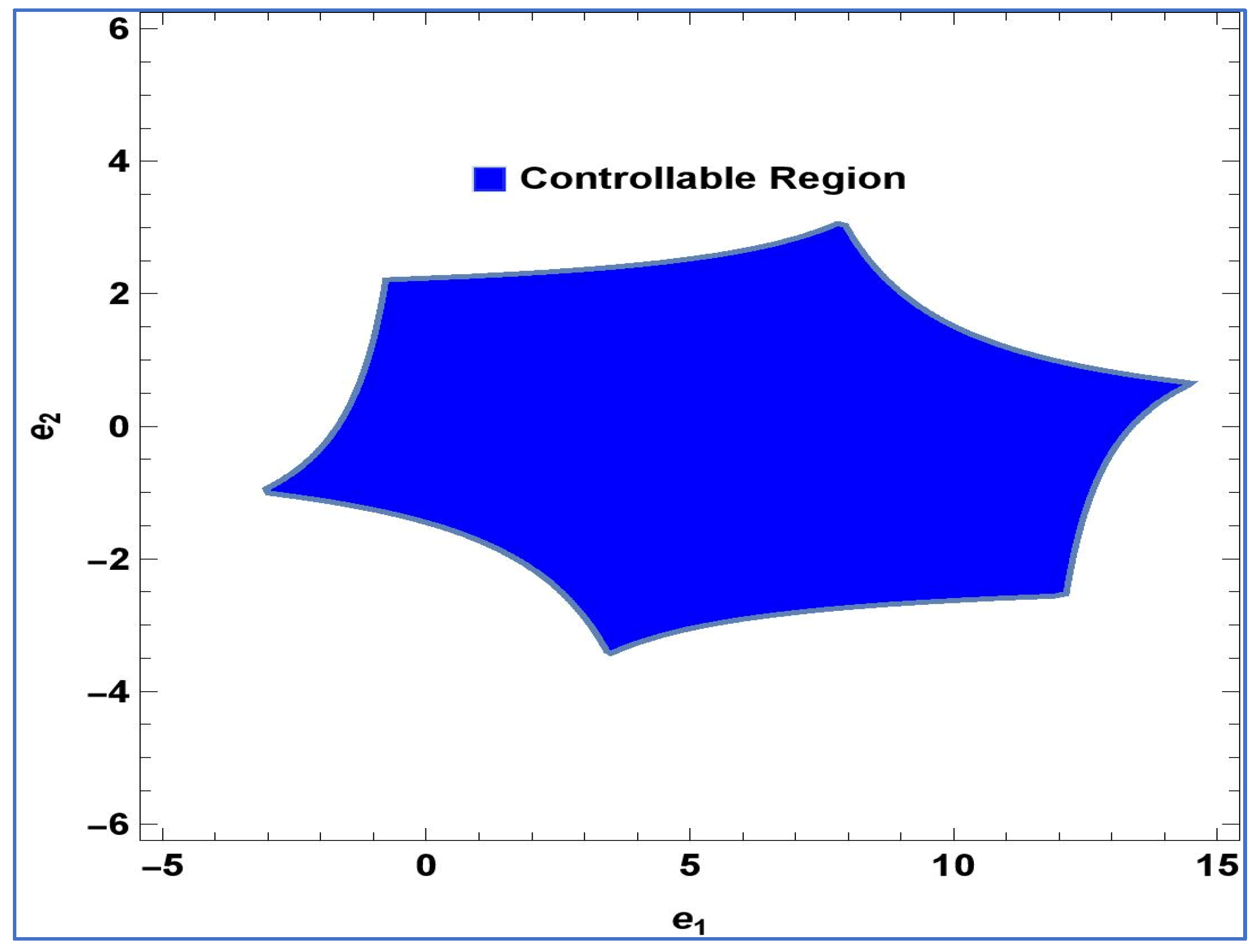
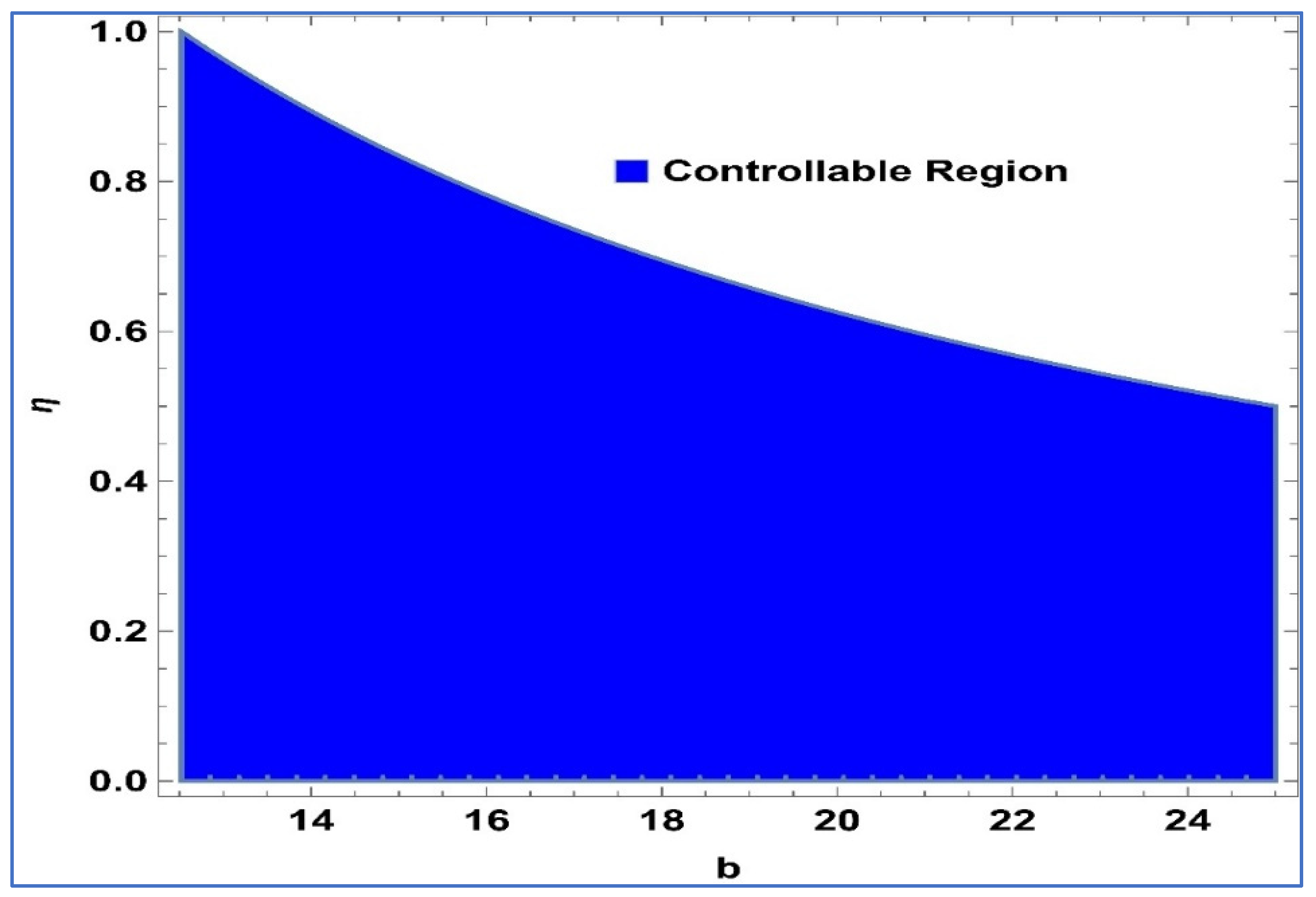
Considering the system’s controllability as described in (24), Henceforth, the Lemma 2 is put forth.

Lemma 2.

The point $\left(x^{*},y^{*}\right)$ in system (24) is a stable sink, should the condition be fulfilled:

$$\begin{array}{l}\left|2+b(c-1)c\eta -\frac{c(-1+a-a{c}^2+a{(c-1)}^{2}k)\eta }{c(k-1)-k}\right|\\ <1+(-k+c(-1+k+(1-a+bc+a{c}^2-b{c}^2+(b\\ -a) {\left(c-1\right)}^2 k)\eta +b(1+a(c-1\left)\right)(c-1)(c\\ +a{\left(c-1\right)}^2 k\left){ \eta }^2\right))/(c(k-1)-k)<2\end{array}$$

For$k=4.57$, $c=0.95$ and$a=4.5$, controllable region of (24) is depicted in Figure 4 in $\eta b$-plane:

Finally, we employ a recently developed strategy for controlling chaos of exponential type to system $\left(4\right)$ as follows [52]:

$$\genfrac{}{}{0pt}{}{x_{n+1}=\mathrm{e}\mathrm{x}\mathrm{p}\left[-{\mathrm{e}}_1\left(x_n-\frac{c\left(1-a+ac\right)}{c+ak-2ack+a{c}^{2}k}\right)\right]x_n\mathrm{e}\mathrm{x}\mathrm{p}\left[\frac{1-x_n}{1+k{y}_n}-\frac{a y_n}{x_n+y_n}\right],}{y_{n+1}=\mathrm{e}\mathrm{x}\mathrm{p}\left[-{\mathrm{e}}_2\left(y_n-\frac{\left(1-c\right)\left(1-a+ac\right)}{c+ak-2ack+a{c}^{2}k}\right)\right]y_n\mathrm{e}\mathrm{x}\mathrm{p}\left[b\left(\frac{x_n}{x_n+y_n}-c\right)\right], }$$

(26)

To, assess the efficacy of the exponential chaos control method in relation to the positive fixed point $\left(x^{*},y^{*}\right)$ within system (4), it is imperative to investigate the local stability of system (26) centered around the same fixed point $\left(x^{*},y^{*}\right)$. To achieve this, the variational matrix $J_E$ $\left(x^{*},y^{*}\right)$ for system (26) is determined through the following procedure, where $e_1$ and $e_2$ are manipulated parameters, and $\left(x^{*},y^{*}\right)$ represents the internal constant solution of system (4):

$$\begin{gathered} J_E\left(x^{\mathrm{*}},y^{\mathrm{*}}\right)= \\ \left(\begin{array}{cc}1+c(a-ac+\frac{(-1+a-ac)\mathrm{c}1}{c+a{(c-1)}^{2}k}-\frac{1+a(c-1)}{c+k-ck})& \frac{ac(c^2-(c-1\left)\right(1+a(c-1)+c\left)k\right)}{c(k-1)-k}\\ b{(c-1)}^2& 1-bc+b{c}^2+\frac{(1+a(c-1\left)\right)(c-1)\mathrm{c}2}{c+a{(c-1)}^{2}k}\end{array}\right). \end{gathered}$$

Furthermore, the computation of the characteristic polynomial for $J_E$ at the point $\left(x^{*},y^{*}\right)$ proceeds as follows:

$$\begin{array}{l}H\left(\xi \right)\\ ={\xi }^2\\ -(2-\left(a-b\right)\left(-1+c\right)c+\frac{c+a\left(c-1\right)c}{c\left(-1+k\right)-k}\\ -\frac{\left(1+a\left(c-1\right)\right)\left(c\left(\mathrm{c}1-e_2\right)+e_2\right)}{c+a{\left(-1+c\right)}^{2}k})\xi +1\\ +\left(b+a\left(-1+b\left(1+a\left(-1+c\right)\right)\left(-1+c\right)\right)\right)\left(-1+c\right)c\\ +\frac{\left(1+a\left(-1+c\right)\right)\left(-e_2+c\left(1+b\left(1+a\left(-1+c\right)\right)\left(-1+c\right)c+e_2\right)\right)}{c\left(k-1\right)-k}\\ -\frac{{\left(1+a\left(c-1\right)\right)}^2\left(c-1\right)c{e}_1{e}_2}{{\left(c+a{\left(c-1\right)}^{2}k\right)}^2}\\ -\frac{\left(1+a\left(c-1\right)\right)\left(c\left(1+b\left(c-1\right)c\right)e_1+\left(c-1\right)\left(-1+a\left(-1+c^2\right)\right)e_2\right)}{c+a{\left(c-1\right)}^{2}k}.\end{array}$$

(27)

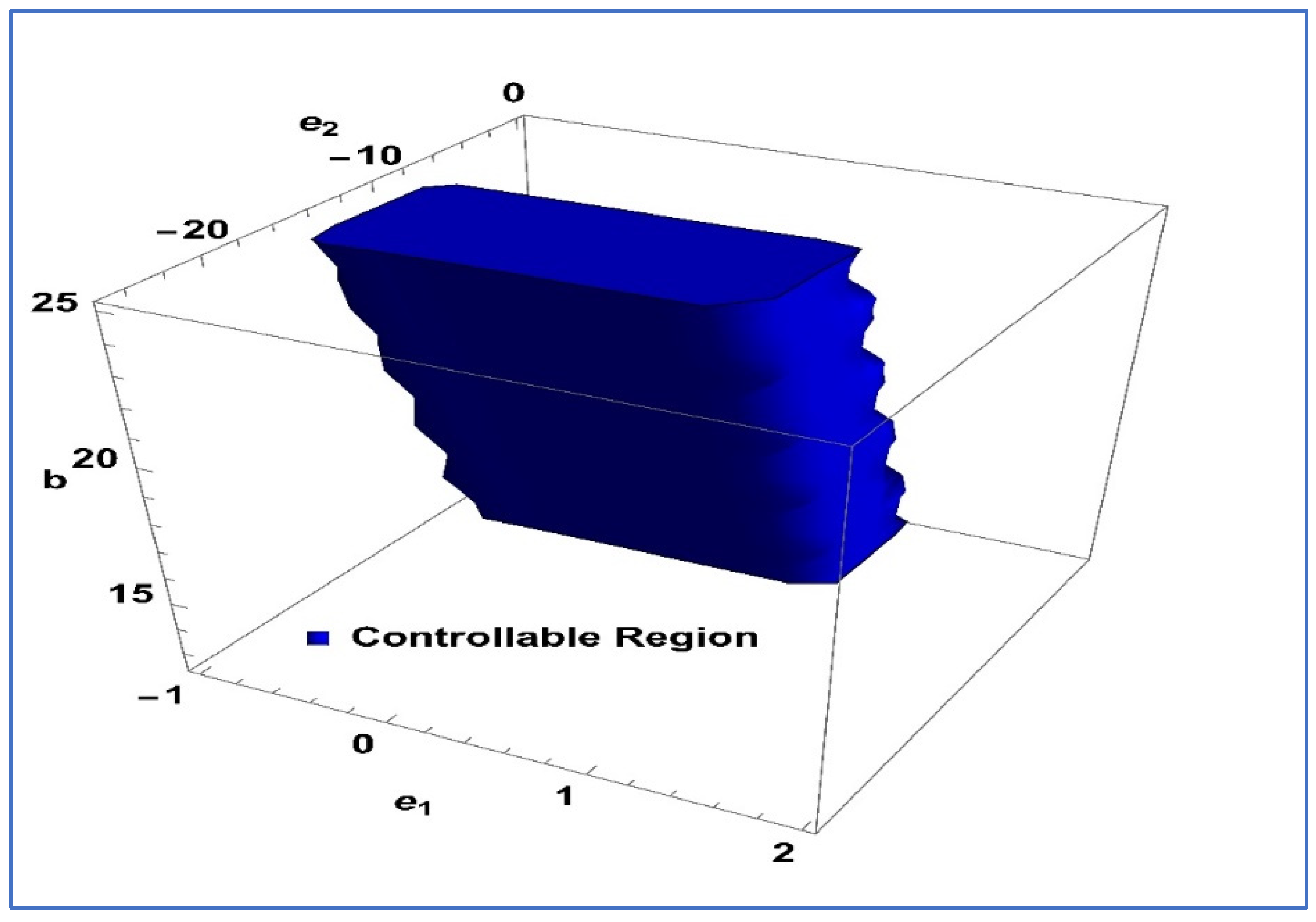
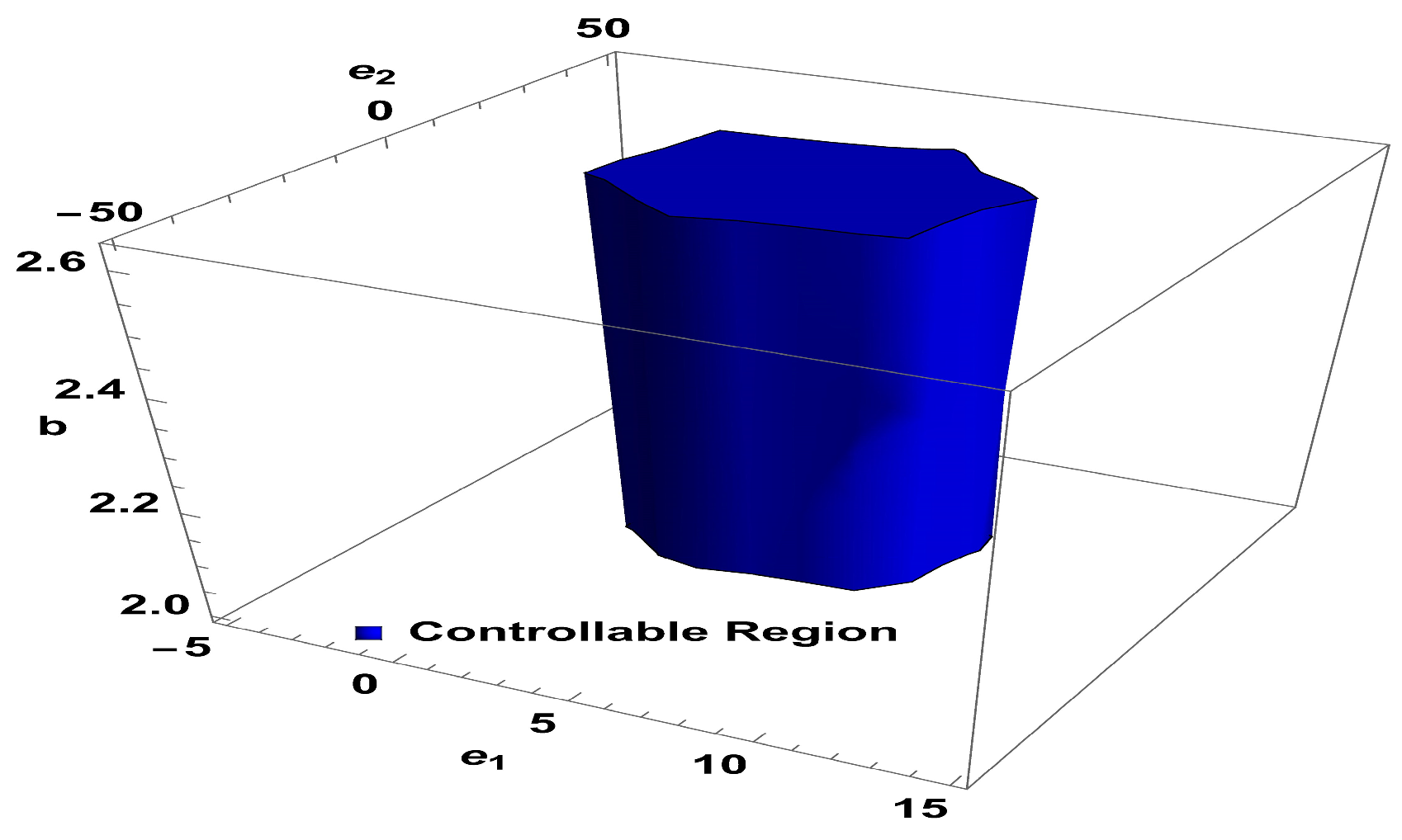
To ensure the controllability of system $\left(26\right)$, the subsequent Lemma 3 is provided.

Lemma 3.

The point $\left(x^{*},y^{*}\right)$ within $system \left(26\right)$ is considered a sink when the following condition is satisfied.

$$\begin{array}{l}\left|2-\left(a-b\right)\left(-1+c\right)c+\frac{c+a\left(c-1\right)c}{c\left(-1+k\right)-k}-\frac{\left(1+a\left(c-1\right)\right)\left(c\left(c1-e_2\right)+e_2\right)}{c+a{\left(-1+c\right)}^{2}k}\right|\\ <2+\left(b+a\left(-1+b\left(1+a\left(-1+c\right)\right)\left(-1+c\right)\right)\right)\left(-1+c\right)c\\ +\frac{\left(1+a\left(-1+c\right)\right)\left(-e_2+c\left(1+b\left(1+a\left(-1+c\right)\right)\left(-1+c\right)c+e_2\right)\right)}{c\left(k-1\right)-k}\\ -\frac{{\left(1+a\left(c-1\right)\right)}^2\left(c-1\right)c{e}_1{e}_2}{{\left(c+a{\left(c-1\right)}^{2}k\right)}^2}\\ -\frac{\left(1+a\left(c-1\right)\right)\left(c\left(1+b\left(c-1\right)c\right)e_1+\left(c-1\right)\left(-1+a\left(-1+c^2\right)\right)e_2\right)}{c+a{\left(c-1\right)}^{2}k}<2.\end{array}$$

For $c=0.27,k=1.1,a=0.73$ and $b=5.5$ controllable region of (26) is depicted in Figure 5 in $e_1{e}_2$-plane.

7. Results and Discussion

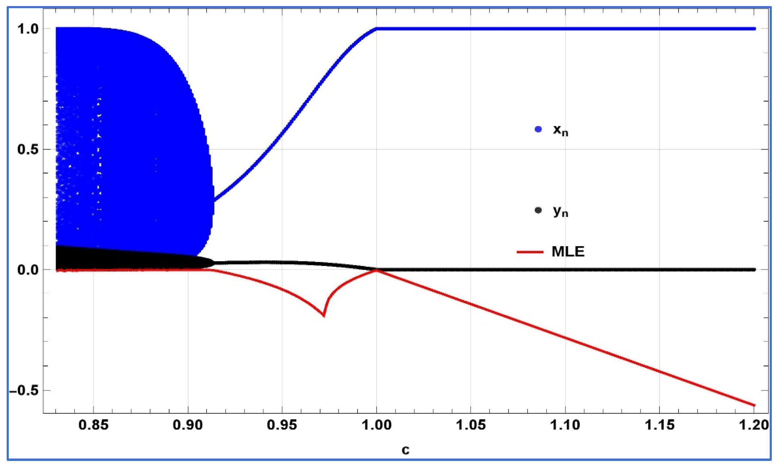
To confirm the presence of transcritical bifurcation, period-doubling bifurcation, Neimark–Sacker bifurcation, and the appropriateness of chaos management techniques, we will illustrate a numerical simulation. Various numerical simulations will be conducted using Mathematica $13.2.$ First, for the verification of emergence of transcritical bifurcation numerically, we chose $k=50$, $a=3.5$, $b=2.8$, and $c\in [0.8,1.2]$, then system (4) experiences transcritical bifurcation about its predator-free fixed point at $c=1$. The bifurcation diagrams, and associated MLE are depicted in Figure 6.

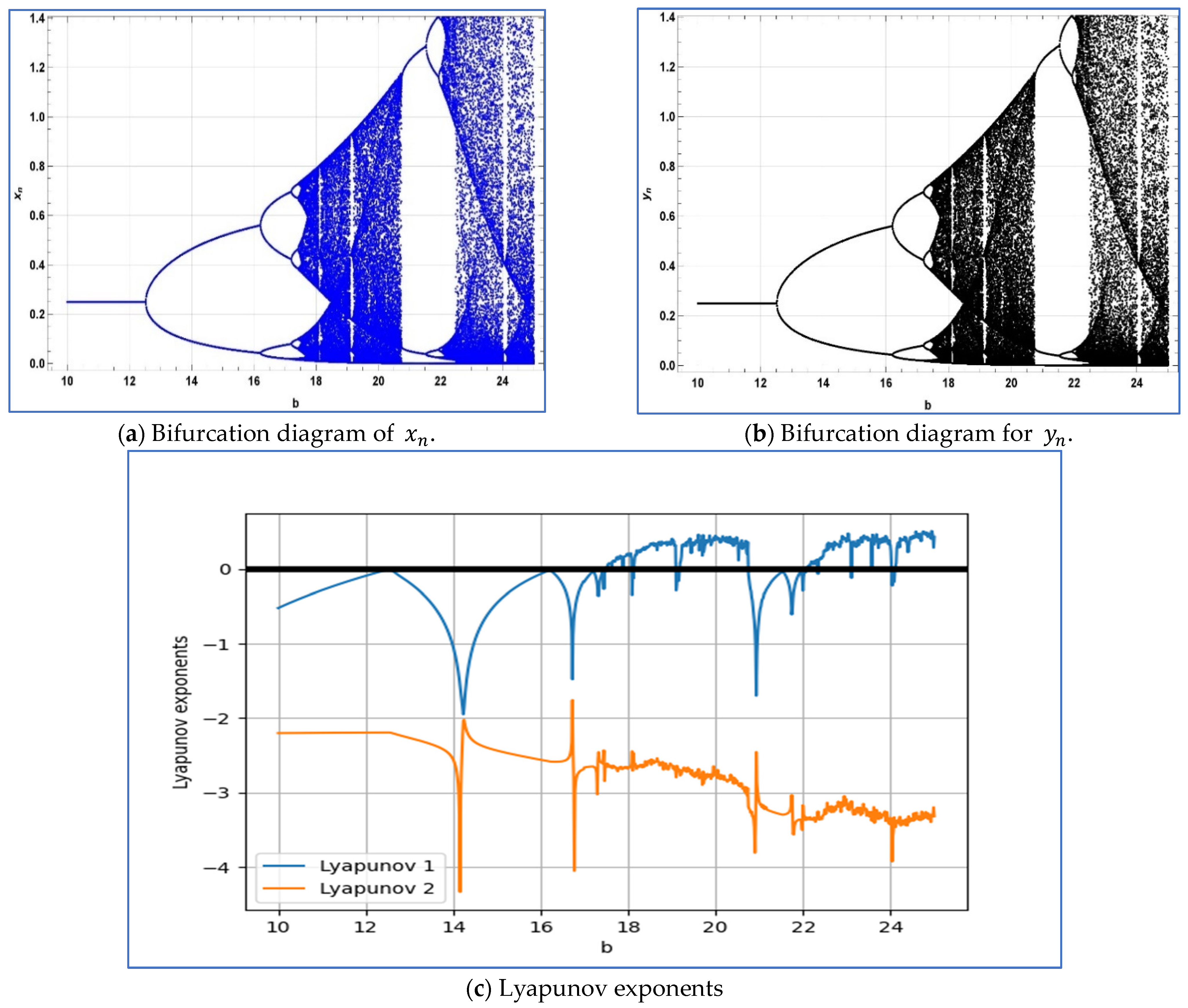
To verify the emergence of period-doubling bifurcation in system $\left(4\right)$ around its unique positive fixed point, we select the parameters$k=0.5, a=0.01, c=0.8$, and$b\in [10,25]$. Subsequently, system (4) exhibits period-doubling bifurcation around its positive fixed point $(0.997751, 0.2494376)$ when the bifurcation parameter b varies within a small neighborhood of $b\equiv b_0=12.5205.$Moreover, for $k=0.5, a=0.01, c=0.8,$ and$b=12.5205$, the Jacobian matrix of system (2.3) is given as follows:

$$\left[\begin{array}{cc}0.1144889& -0.0072871\\ 0.50082& -1.00328\end{array}\right].$$

On the other hand, the eigenvalues of above Jacobian matrix are given as follows $-1$, and$0.11121428170014735$. In this case, the bifurcation diagrams and corresponding Lyapunov exponents are depicted in Figure 7a–c.

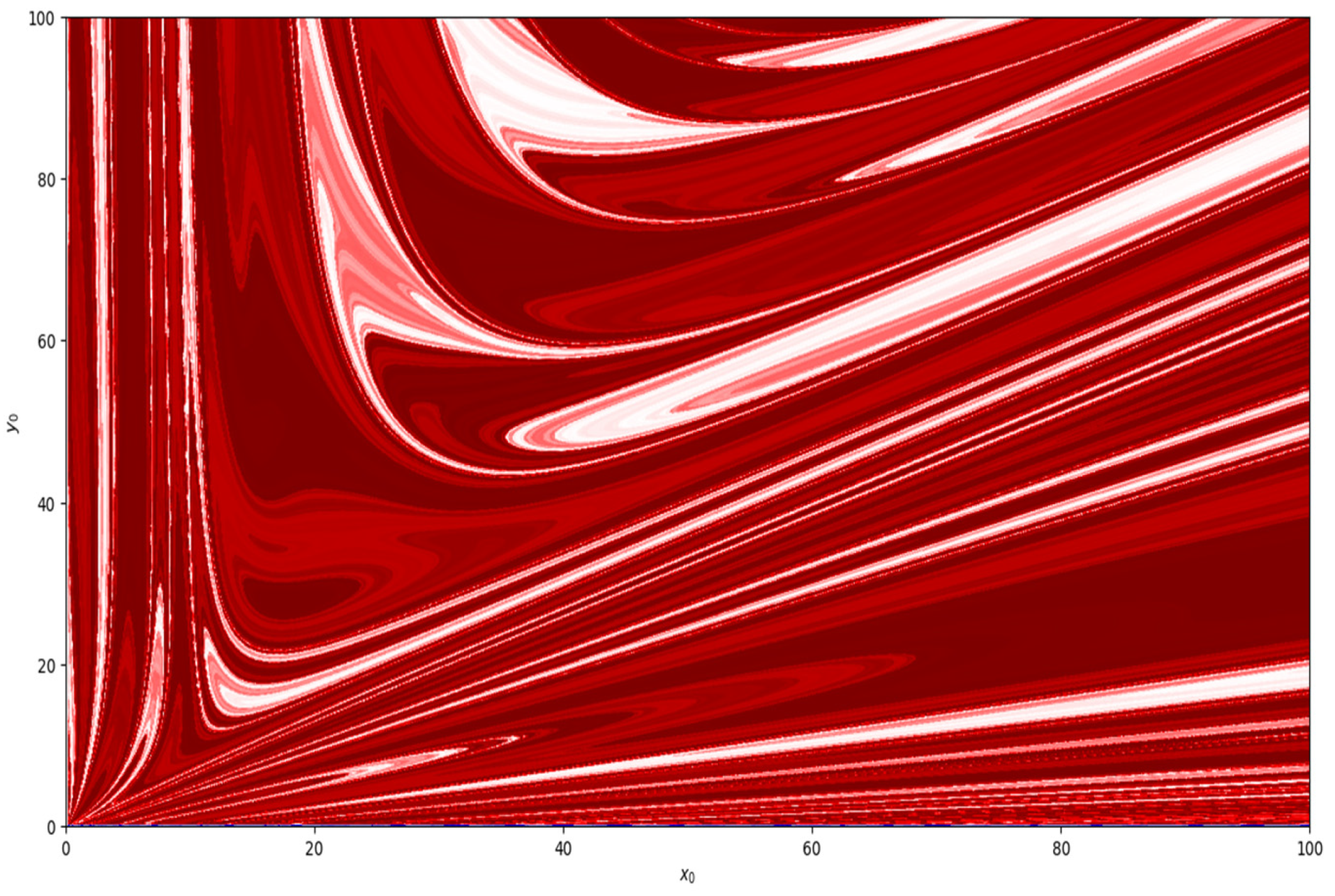
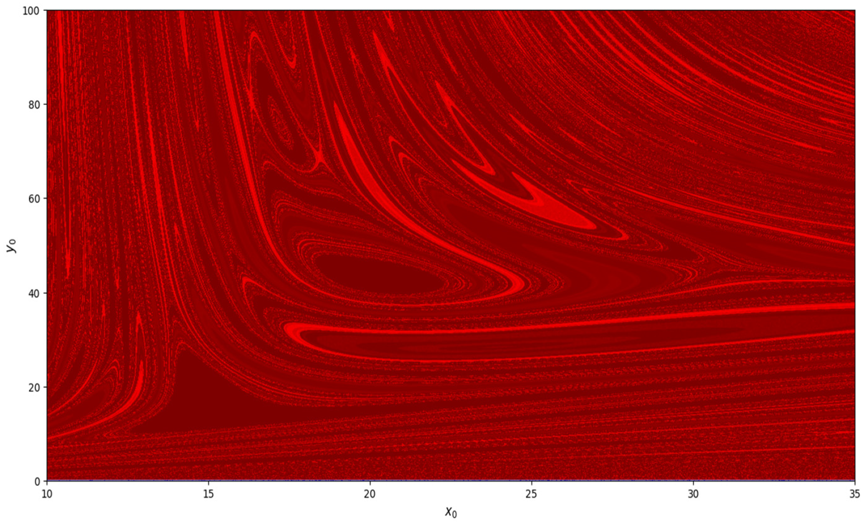
Moreover, taking parametric values $a=0.01$, $k=0.5$, $c=0.8$, and $b=17.483$, basin of attraction is shown in Figure 8. Similarly, basin of attraction for $a=0.01$, $k=0.5$, $c=0.8$, and $b=22.08$ is depicted in Figure 9.

Next, we discuss the relevance of period-doubling bifurcation to chaos control. Initially, we validate the hybrid control strategy outlined in Equation $\left(24\right)$. To achieve this, we define the system governed by Equation (24) with the values $k=0.5, a=0.01$, and$c=0.8$. We keep the control parameter $\eta$ within the permissible range of [0, 1] and vary the bifurcation parameter b within the chaotic region [12.5205, 25] maintaining the specified fixed values. Figure 10 illustrates the fluctuation of the stability area on the $\eta b$-plane concerning the bifurcation parameter $b$ and control parameter$\eta$.

Next, to determine the validity of exponential control, we take the values $k=0.5, a=0.01$, $c=0.8$ and $b\in [12.5205,25]$ for the system (26), then Figure 11 illustrates the feasible region corresponding to system (26) in the $e_1{e}_{2}b$-space.

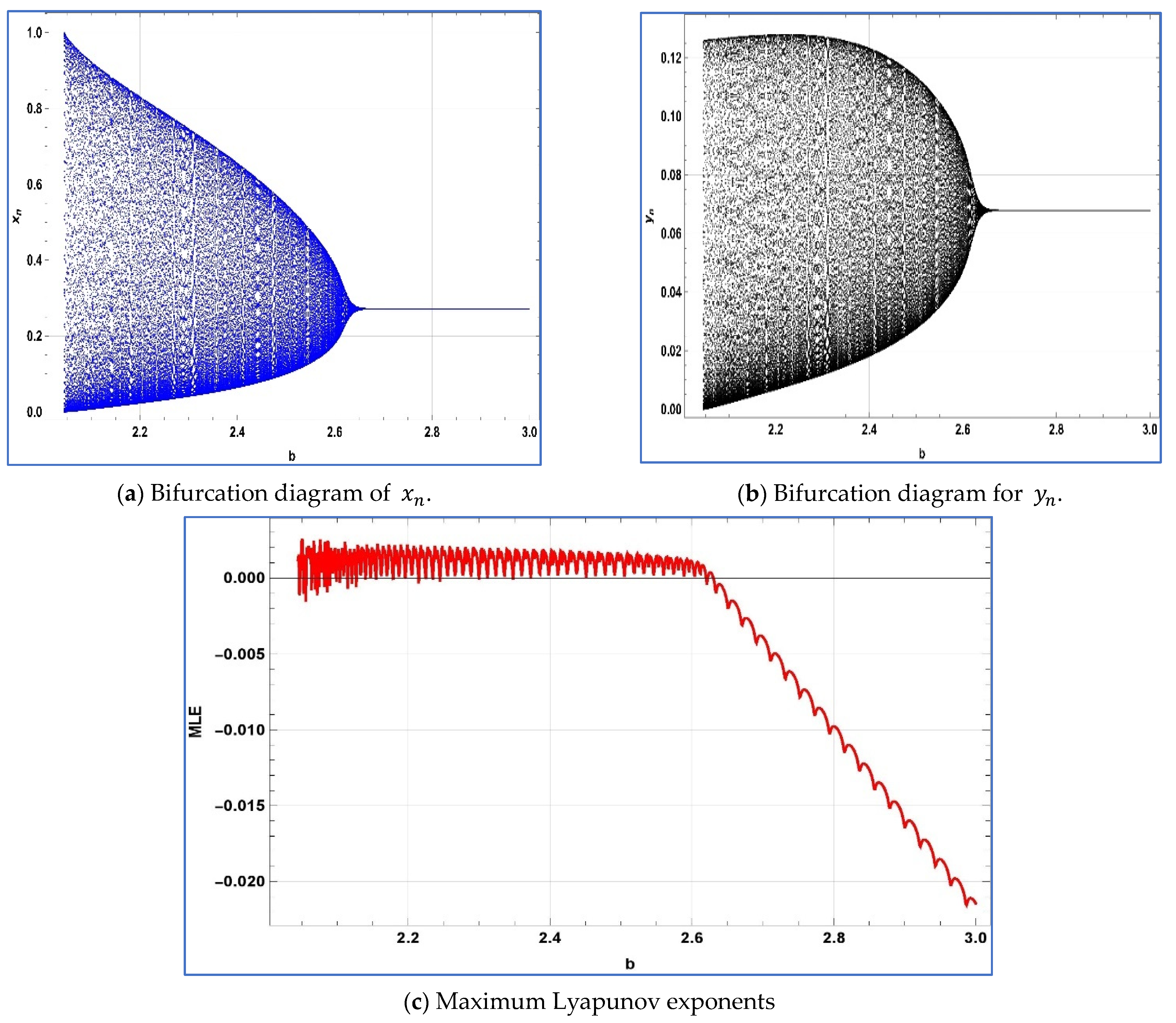
Now, we confirm that torus bifurcation occurs for the system represented by system $\left(4\right)$. In order to accomplish this, we set the initial condition $(x_0, y_0)=(0.271, 0.0678)$ and choose particular parameter values for system (4), namely,$k=0.6, a=3.5$ and $c=0.8$. Next, system (4) experiences a crucial bifurcation parameter value of $b_1$ $=2.6267562614$, leading to a Neimark–Sacker bifurcation at the point$\left(x*, y* \right)=\left(0.271493,0.067\right).$ Additionally, when $k=0.6$, $a=3.5, c=0.8$ and $b\in (2, 3)$ the characteristic polynomial for the variational matrix of system (4) is computed as follows:

$$p\left(\tau \right)={\tau }^2-1.878849432949988\tau +1$$

Subsequently, the multipliers of the variational matrix, denoted as the roots of $p\left(\tau \right)$, are expressed as ${\tau }_1=0.9394247+0.3427553i$ and${\tau }_2=0.9394247-0.3427553i$ while ensuring $\left|{\tau }_1\right|=\left|{\tau }_2\right|=1$ in accordance with the conditions stipulated in Theorem$3$ under the condition, the derivatives of $\left(\frac{d}{d\tilde{b}}\left|{\tau }_{\mathrm{1,2}}\right|\right)$ with respect to $\tilde{b}=0$ are calculated as:

$$\frac{{\left(c-1\right)}^{2}c(ac+k+a(1+a(c-1)\left)\right(c-1\left)k\right)}{2c(k-1)-2k}=-0.05693913043478259.$$

The condition

$$2-\left(a-b_1\right)\left(c-1\right)c+\frac{c+a\left(c-1\right)c}{c\left(k-1\right)-k}=-1.5088695652173911$$

holds true. Consequently, the system satisfies the non-degeneracy and non-resonance conditions. Hence, it can be inferred that $(a,b,c,k) \in S_{NB}$, and all the conditions specified in Theorem 3 are met. Additionally, Figure 12 illustrates the bifurcation diagrams and the maximum Lyapunov exponent (MLE) of the system for $b\in \left[2, 3\right].$

In the conclusion of this part, we confirm the efficiency of chaos control techniques in the context of Neimark–Sacker bifurcation. First, we evaluate if a hybrid control method is acceptable by assuming that the system has values of$k=0.6, a=3.5$ and $c=0.8$ in system (24). The controllability interval changes inside the chaotic region $[2, 2.62675626]$ when the bifurcation parameter $b$ changes. Interestingly, the duration of the controllability interval is shown to increase with changing the value of the bifurcation parameter at the left end of the chaotic zone. Figure 13, shows the variation in controllability with respect to control parameter $b$. The findings show that chaotic behavior in the system may be efficiently controlled by using a hybrid control method.

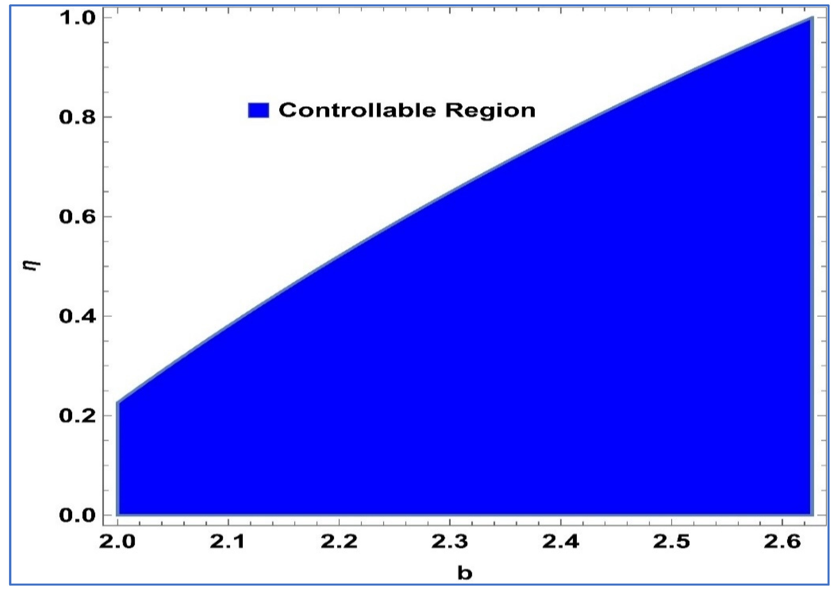
Next, to determine the validity of exponential control, we take the values $k=0.6, a=3.5$, $c=0.8$ and b ∈ [2, 2.62676] for system (26), then Figure 14 illustrates the feasible region corresponding to system (26) in the $e_1{e}_{2}b$-space.

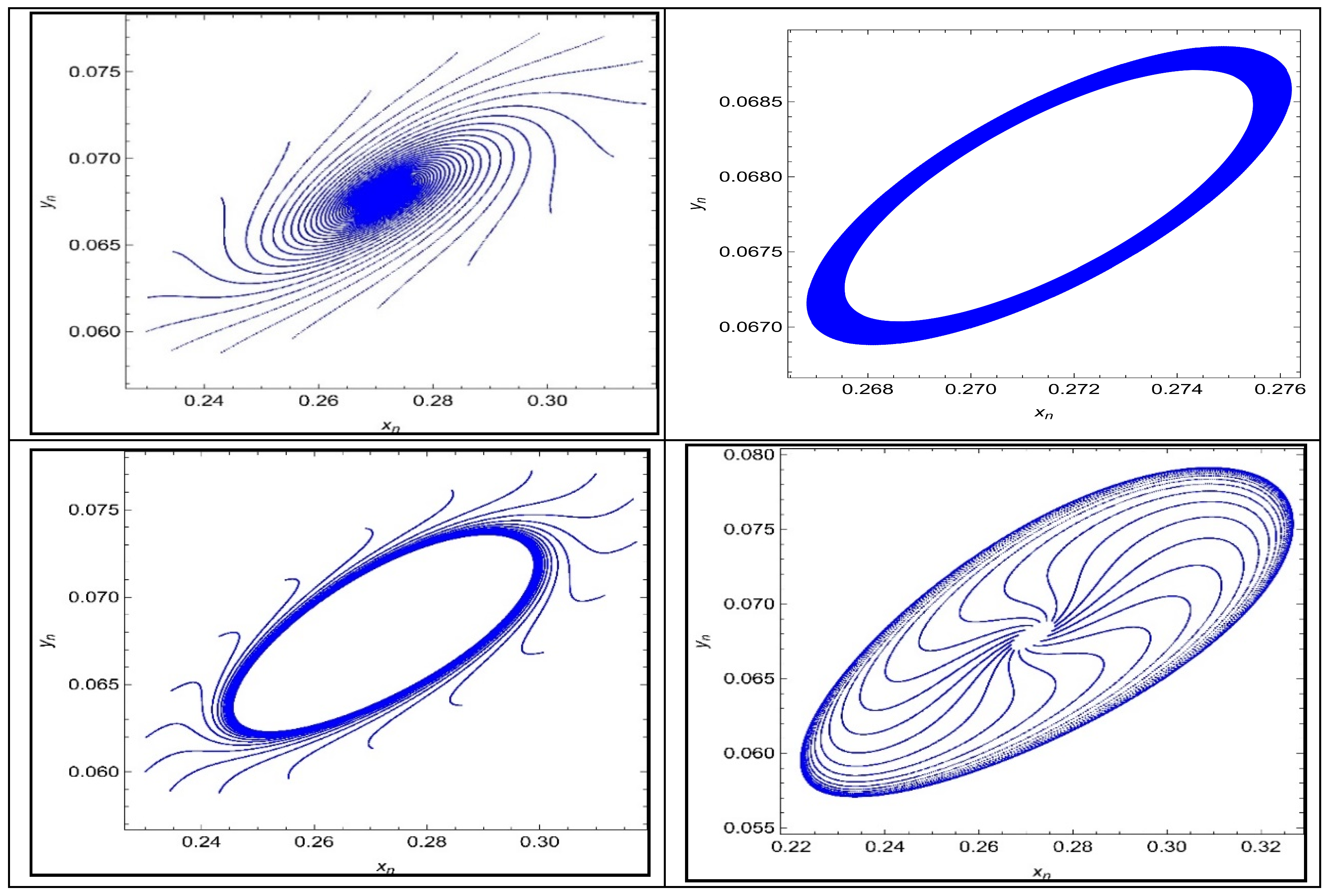
Next, some phase portraits of system (4) are presented in Figure 15 taking different values of bifurcation parameter $b$.

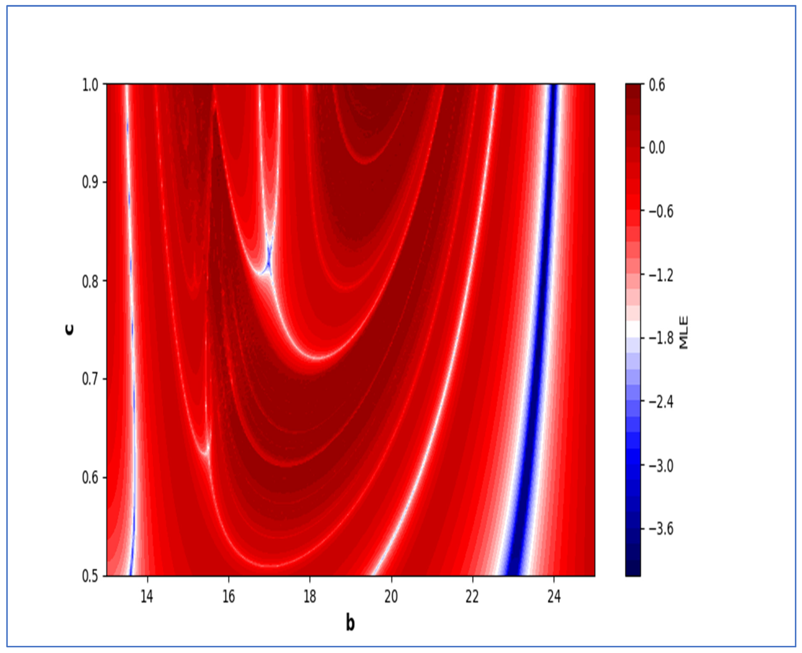
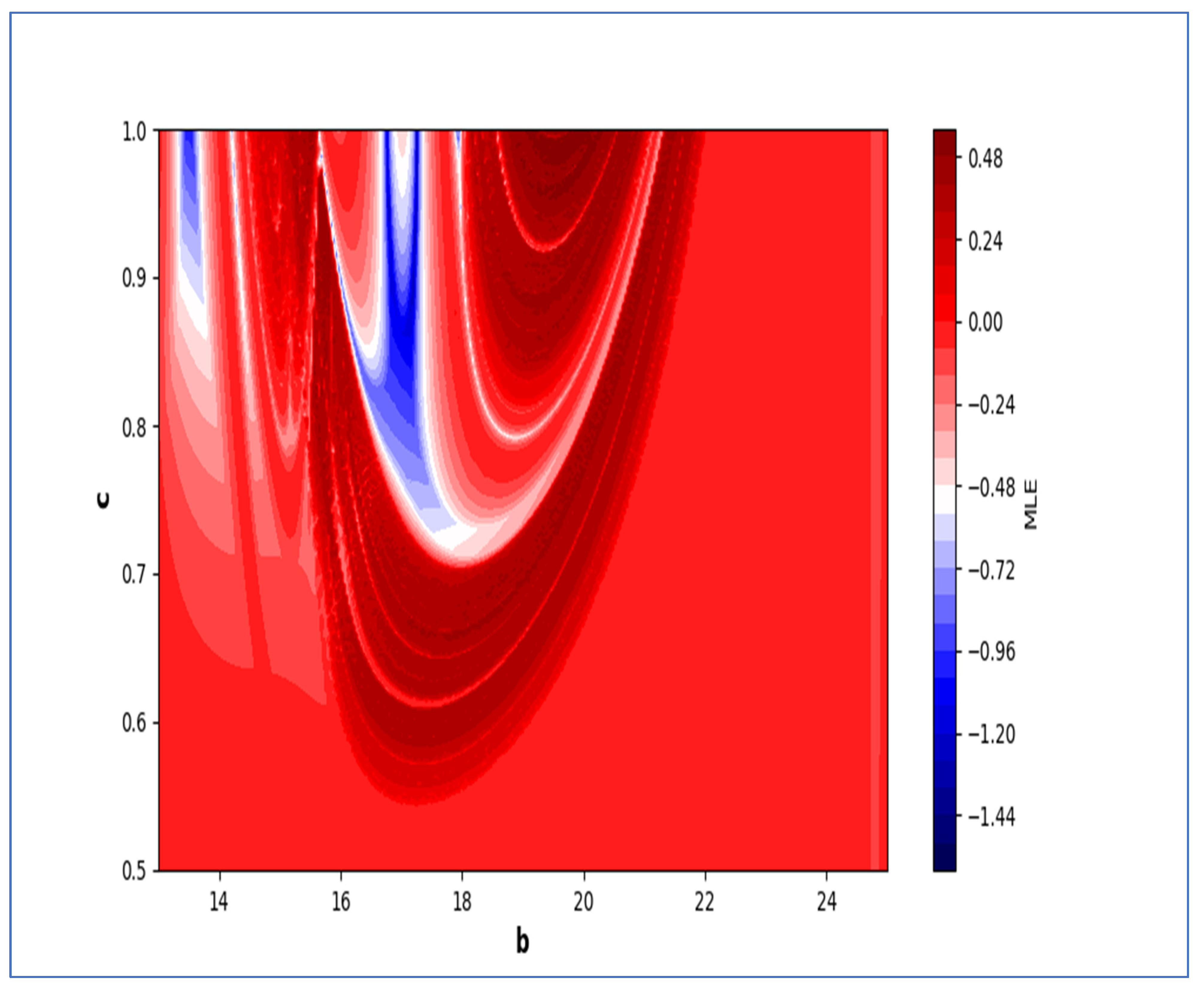
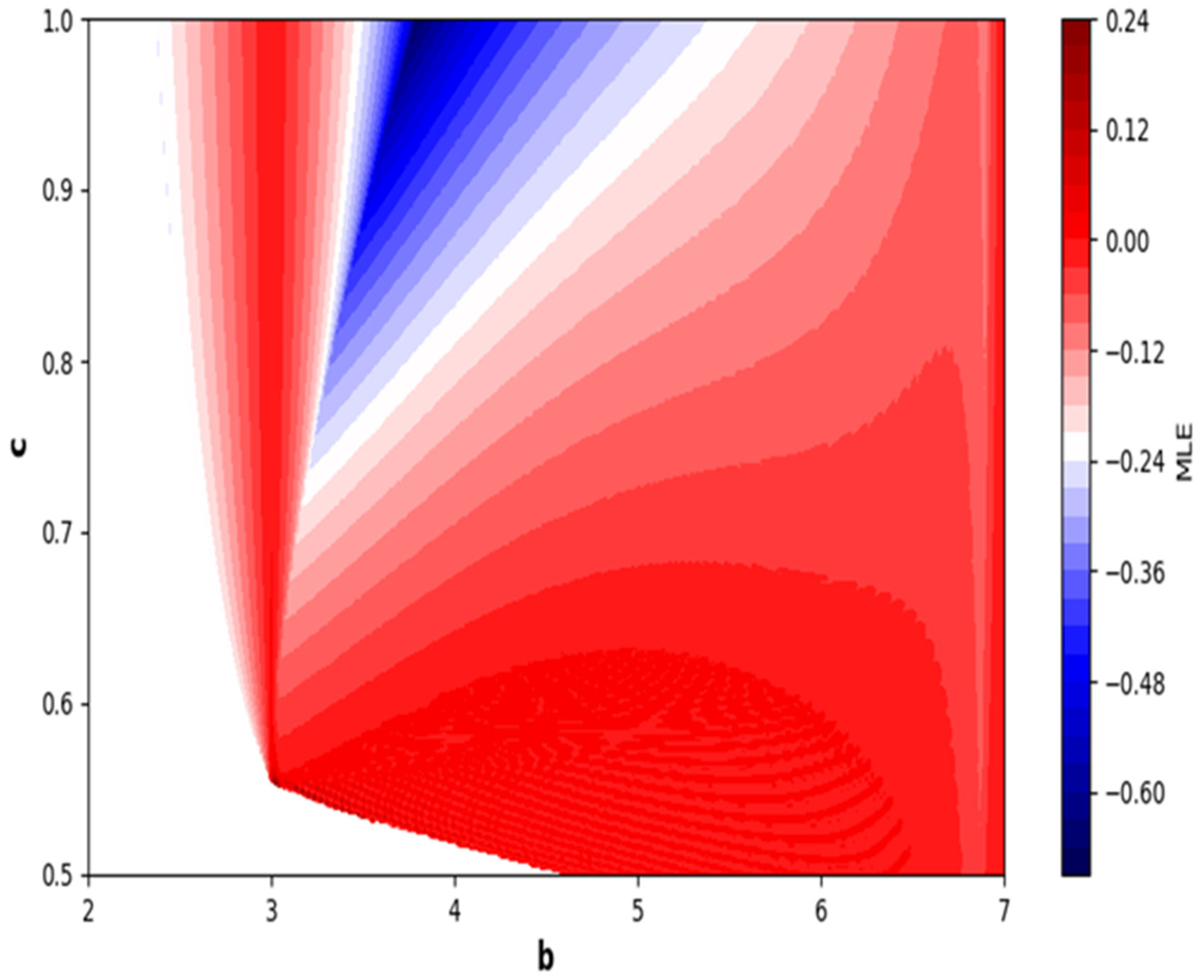
In the end, we focused on two-parameter dynamics of system (4) based on the variation in the maximum Lyapunov exponents and Lyapunov spectrum. For this, two parameters $13<b<25$ and $0.5<c<1$. On the other hand, $a$ is kept fixed as $a=0.01$. In order to check the impact of fear level $k$ on the dynamics of prey-predator interaction, very low and high fear levels are selected, that is, $k=0.000001$ (a very low level), and $k=1000$ (a high fear level).

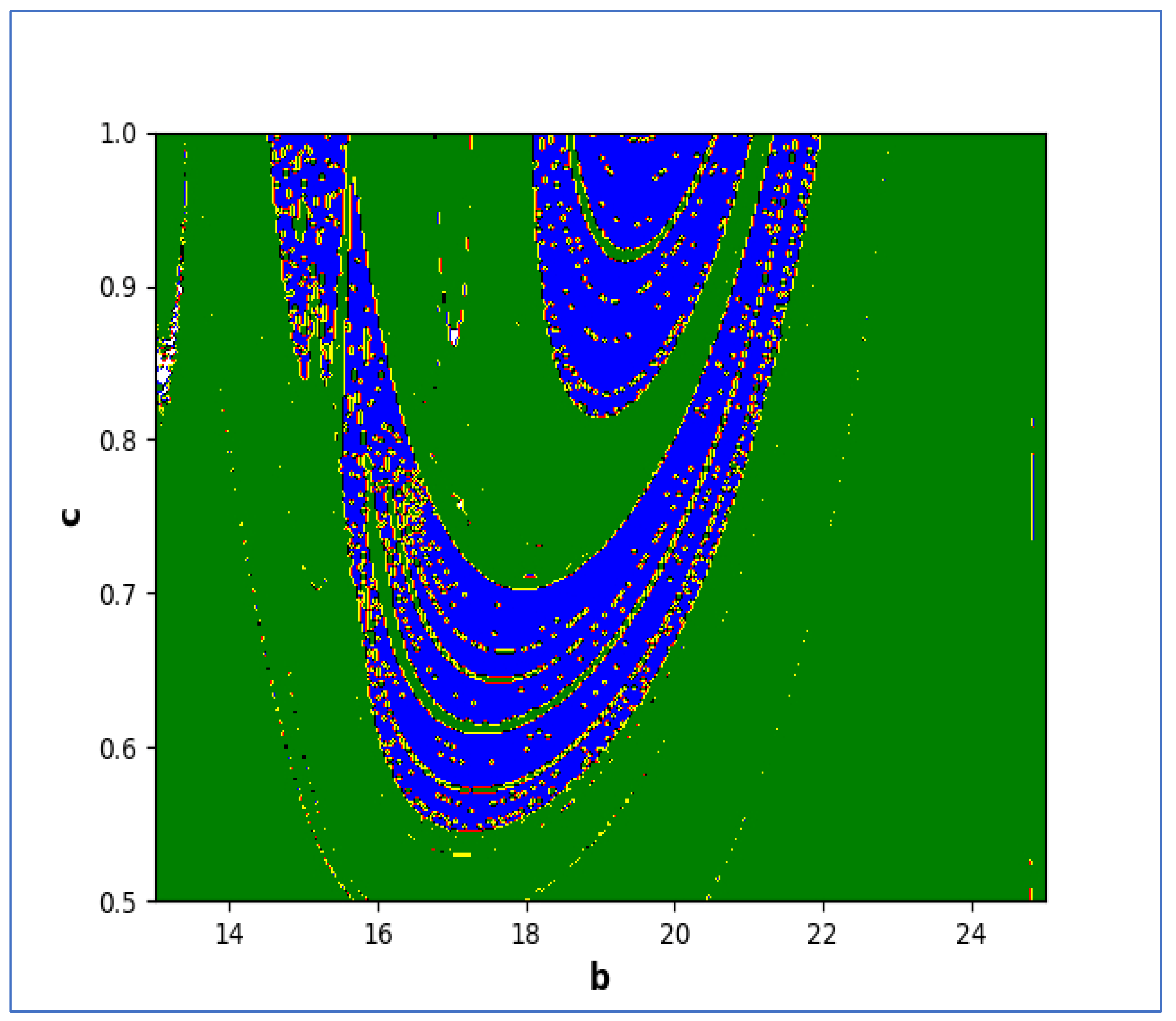
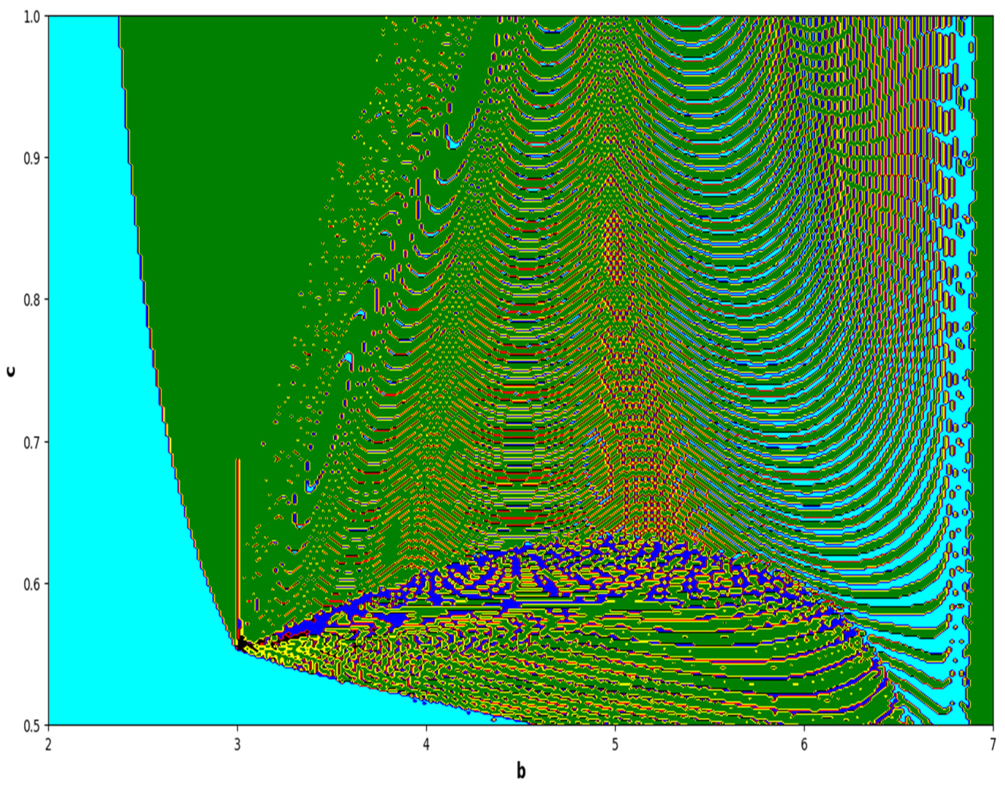
Moreover, two-parameter based the maximum Lyapunov exponents dynamics is presented in Figure 16 with $k=0.000001$ and $a=0.01$. On the other hand, the corresponding Lyapunov spectrum is presented in Figure 17. Similarly, two-parameter based the maximum Lyapunov exponents dynamics is presented in Figure 18 with $k=1000$ and $a=0.01$. 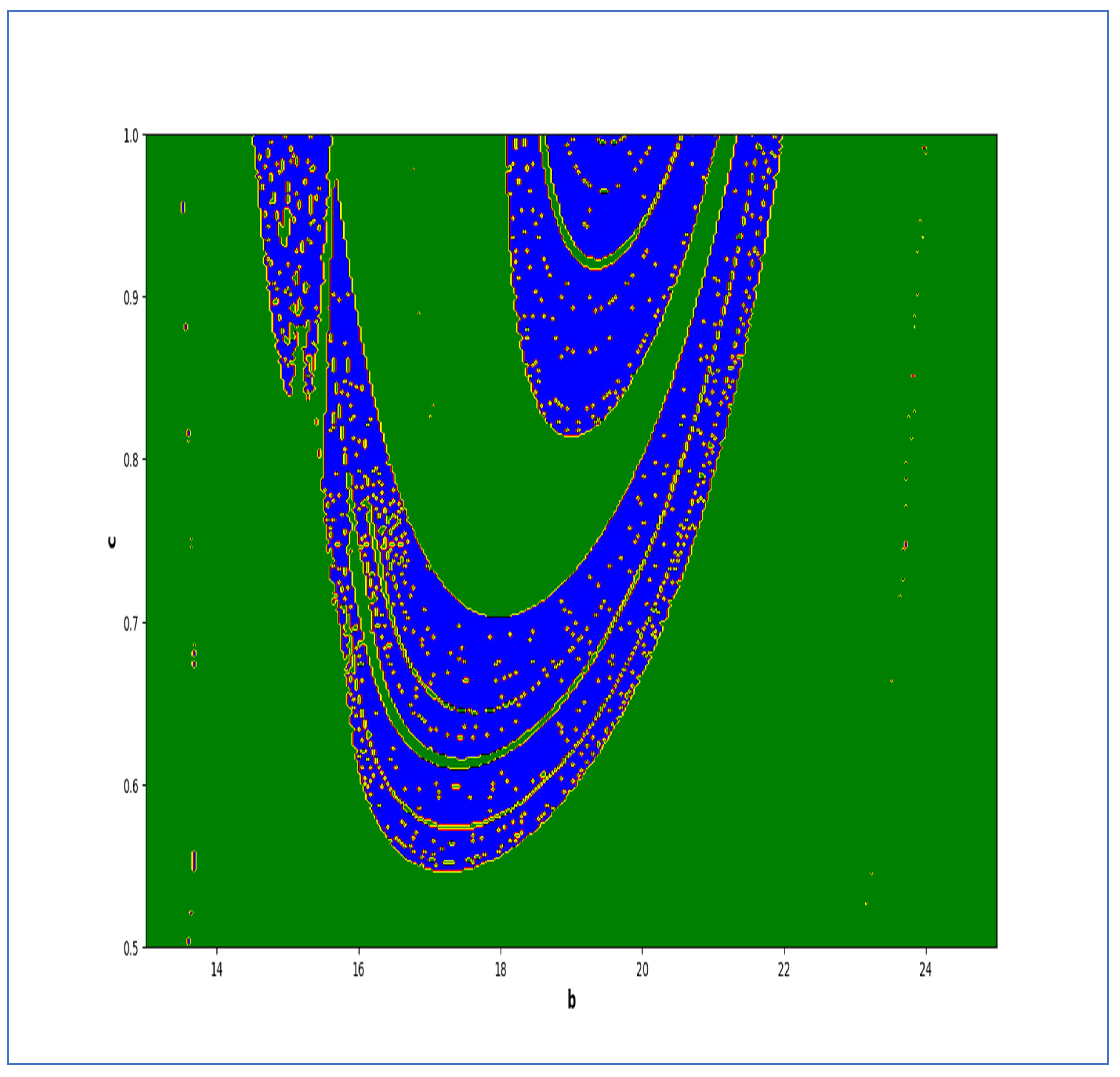On the other hand, the corresponding Lyapunov spectrum is presented in Figure 19.

The colors regions in Figure 17 and Figure 19 corresponding to the Lyapunov spectrum are described as follows: $L2<0<L1$ (white region) corresponds to chaotic attractor, $0<L2<L1$ (blue region) corresponds to chaotic attractor, $L2<L1<0$ (red region) corresponds to stable region, $L2=L1<0$ (black region) corresponds to periodic point of focus type, $L2=L1=0$ (yellow region) corresponds to quasiperiodic region, and $L2<L1=0$ (green region) corresponds to invariant circle, where $L1$ and $L2$ are the first and the second Lyapunov exponents.

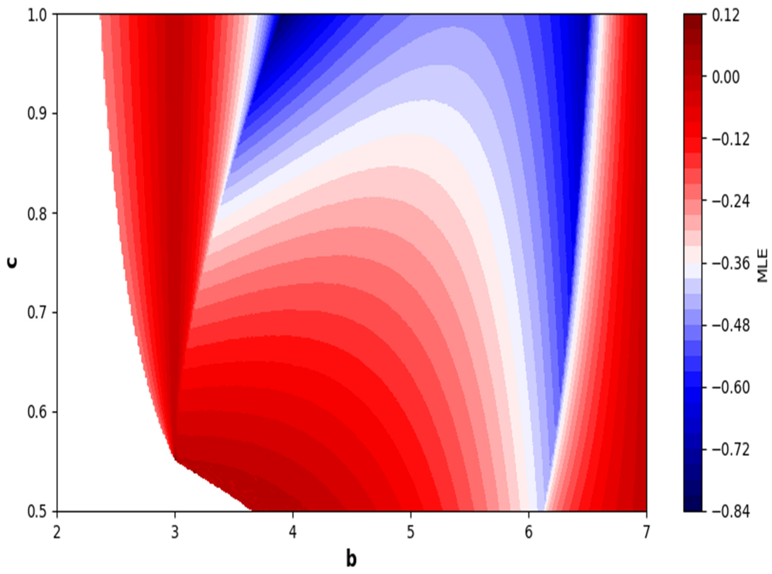
Next, it must be noted that in above two-parameter dynamics the value of parameter $a$ is taken as $a=0.01$, which is ecologically equivalent to a low predation rate for predator–prey interaction. In order to consider the remaining case, that is, when the predation rate has some value greater than one, we consider $a=2.5$. Furthermore, for low and high levels of fear, $k$ is taken as $k=0.9$ for a low level of fear, and $k=500$ for a high level of fear. For $a=2.5$ and $k=0.9$, the two-parameter MLE is depicted in Figure 20. 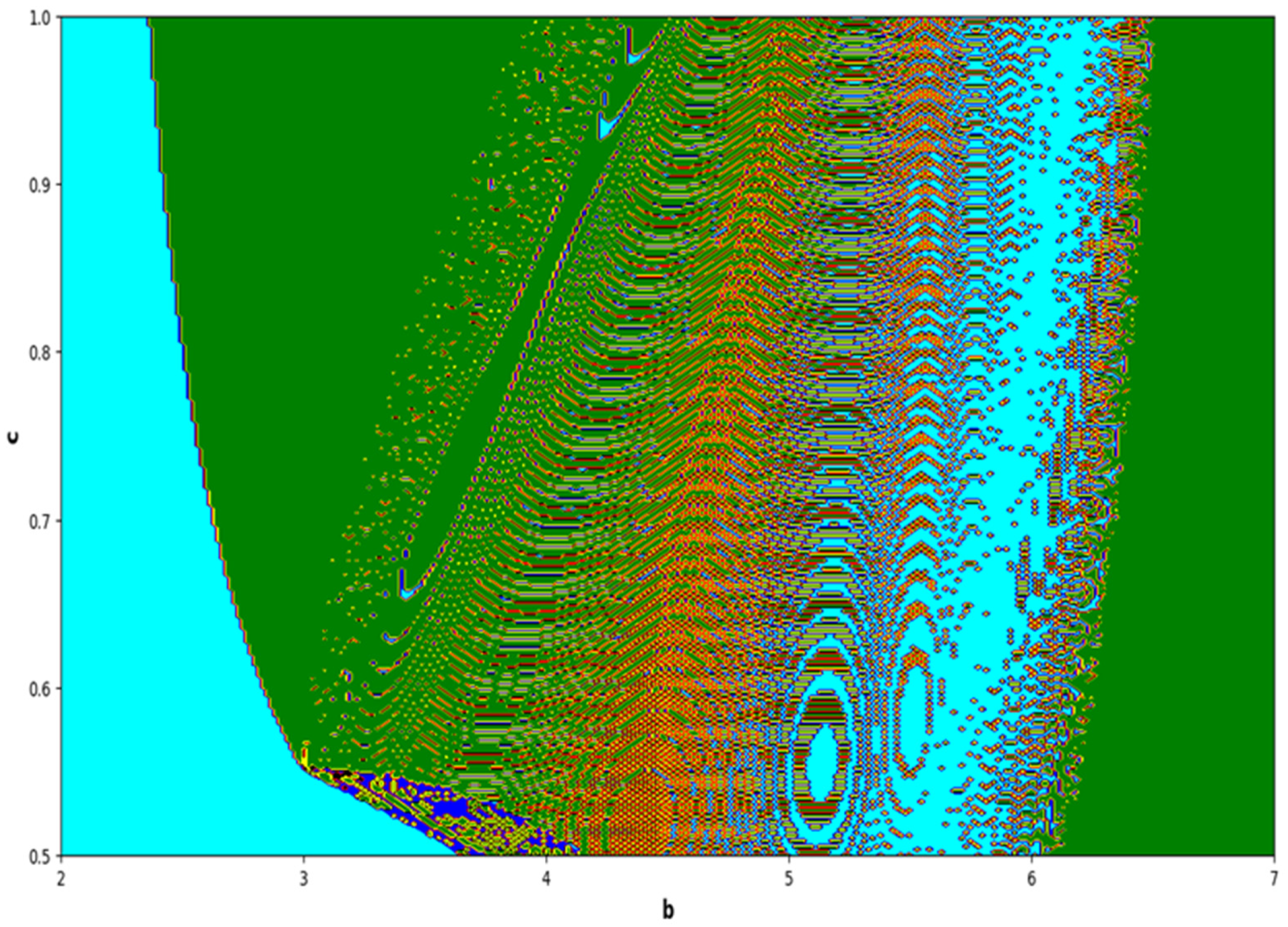On the other hand, the corresponding Lyapunov spectrum is depicted in Figure 21. Similarly, for $a=2.5$ and $k=500$, the two-parameter MLE is depicted in Figure 22. On the other hand, the corresponding Lyapunov spectrum is depicted in Figure 23.

The colors regions in Figure 21 and Figure 23 corresponding to the Lyapunov spectrum are described as follows: $L2<0<L1$ (cyan region) corresponds to chaotic attractor, $0<L2<L1$ (blue region) corresponds to chaotic attractor, $L2<L1<0$ (red region) corresponds to stable region, $L2=L1<0$ (black region) corresponds to periodic point of focus type, $L2=L1=0$ (yellow region) corresponds to quasiperiodic region, and $L2<L1=0$ (green region) corresponds to invariant circle, where $L1$ and $L2$ are the first and the second Lyapunov exponents.

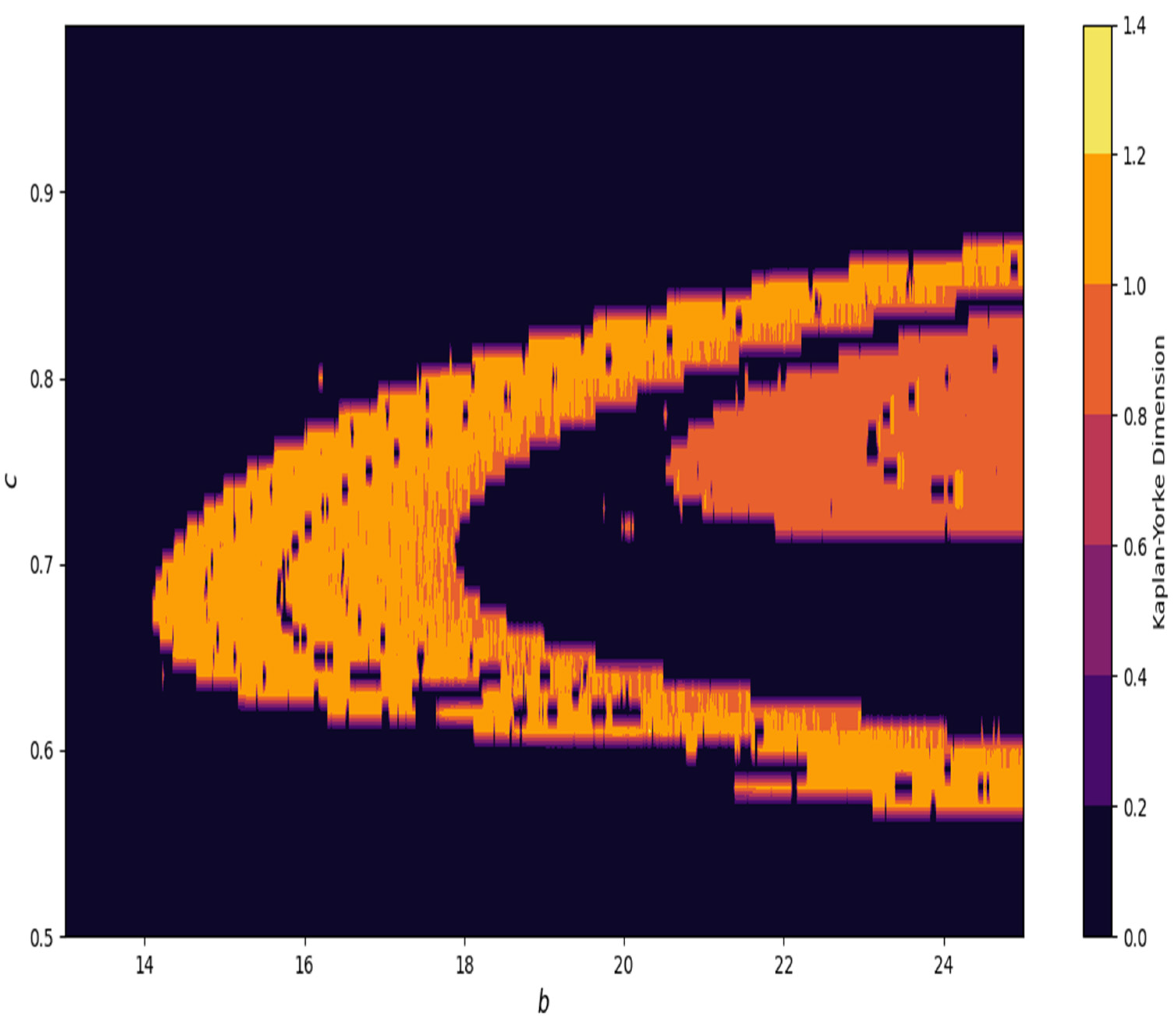
Furthermore, in Figure 24, at $\left(\mathrm{b},\mathrm{c}\right)\in \left[13,25\right]\times [0.5,1]$ and $\mathrm{k}=0.5$, the Kaplan–Yorke dimension is depicted in system (4).

8. Concluding Remarks

Examining the effects of fear on the prey community has significant implications for understanding predator–prey natural interactions, which act as an important factor to understand the dynamics of such ecosystems comprehensively. Our research examines the effect of predator-induced fear on prey populations and their role in varying levels of fear interacting with environmental factors and the fluctuating behavior of the system. It is investigated that low levels of fear coupled with low predation rates reflect and increase the chaotic behavior of the predator–prey interaction. On the other hand, a high level of fear coupled with a low victimization rate stabilizes the system. Consequently, it provides a platform for researchers and ecologists to further investigate other environmental parameters that directly or indirectly affect the fear effect. A predator–prey model with non-overlapping generations was chosen to implement the fear effect and investigation related to its qualitative behavior. The proposed model is ecologically well-posed and meaningful because it preserves the positivity of non-equilibrium solutions for all positive parametric values. Further investigation involves the existence of biologically feasible fixed points and local asymptotic behavior of the system around these equilibrium states. Moreover, codimension-one type bifurcations such as transcritical bifurcation, period-doubling bifurcation, and Neimark–Sacker bifurcation are studied with implementation of standard techniques of normal forms of bifurcation theory. To deal with the unpredictability caused by the interacting species, we use some techniques concerning chaos control, which help us to understand and control uncertainty in the proposed system. This study contributes to our better understanding of predator–prey interactions and highlights how different environmental factors affect ecosystem stability. Two-parameter dynamics particularly with implementation of Lyapunov diagram construction and the depiction of the maximum Lyapunov exponents are implemented to better understand the chaotic behavior of the model with respect to its low and high levels of fear.

Moreover, in Figure 16, it can be observed from the graph that when levels of fear are low, the maximum Lyapunov exponents (MLE) exhibit positivity, which is indicated by the red region. This implies that the model exhibits chaotic behavior. Consequently, the prey population experiences a rapid growth due to the absence of fear, resulting in an unstable prey dynamics. As a result of this instability, predators may adapt their strategies, leading to fluctuations in the prey population. The concentric semicircular lines in the graph depict the periodic patterns of the model. Moving on to Figure 18, it can be noted that when threat levels are high, the maximum Lyapunov exponents tend to display negativity predominantly in the blue region. This negative value indicates a stable dynamics in the system. This indicates that the number of animals being hunted is controlled because of the powerful impact of dangers, leading to more consistent relationships between predators and their prey. Furthermore, as the number of prey animals becomes more foreseeable, it can result in stabilization of predator populations. The circular lines that form concentric patterns on the graph draw attention to regions where the system demonstrates recurring patterns. It must be noted that low and high predation rates also play crucial role for emergence of chaotic behavior under low and high fear levels. In the case of a high predation rate, system is more chaotic with an increased level of fear, and less chaotic with a low level of fear (see Figure 20, Figure 21, Figure 22 and Figure 23). Moreover, fractal and complex behavior of the model is depicted in Figure 24, in which Kaplan–Yorke dimension is plotted in two-parameter plane. Our current approach is theoretical, aiming to explore the impact of fear within the established framework of [43]. Future work could incorporate data to parameterize the fear effect term for a more realistic representation.