Article

Novel Hopf Bifurcation Exploration and Control Strategies in the Fractional-Order FitzHugh–Nagumo Neural Model Incorporating Delay

1
School of Mathematics and Statistics, Henan University of Science and Technology, Luoyang 471023, China
2
Guizhou Key Laboratory of Economics System Simulation, Guizhou University of Finance and Economics, Guiyang 550025, China
*
Author to whom correspondence should be addressed.
Fractal Fract. 2024, 8(4), 229; https://doi.org/10.3390/fractalfract8040229
Submission received: 21 February 2024 / Revised: 4 April 2024 / Accepted: 10 April 2024 / Published: 15 April 2024
(This article belongs to the Special Issue Analysis and Control of Fractional-Order Delay Coupling Networks)

Abstract

:
In this article, we propose a new fractional-order delay-coupled FitzHugh–Nagumo neural model. Taking advantage of delay as a bifurcation parameter, we explore the stability and bifurcation of the formulated fractional-order delay-coupled FitzHugh–Nagumo neural model. A delay-independent stability and bifurcation conditions for the fractional-order delay-coupled FitzHugh–Nagumo neural model is acquired. By designing a proper P D p controller, we can efficaciously control the stability domain and the time of emergence of the bifurcation phenomenon of the considered fractional delay-coupled FitzHugh–Nagumo neural model. By exploiting a reasonable hybrid controller, we can successfully adjust the stability domain and the bifurcation onset time of the involved fractional delay-coupled FitzHugh–Nagumo neural model. This study shows that when the delay crosses a critical value, a Hopf bifurcation will arise. When we adjust the control parameter, we can find other critical values to enlarge or narrow the stability domain of the fractional-order delay-coupled FitzHugh–Nagumo neural model. In order to check the correctness of the acquired outcomes of this article, we present some simulation outcomes via Matlab 7.0 software. The obtained theoretical fruits in this article have momentous theoretical significance in running and constructing networks.

1. Introduction

The human brain consists of thousands of neurons that are connected with each other in a very complex network of neurons [1]. In order to grasp the inherent essence of neurons, many researchers have shown significant interest in establishing appropriate neural network models to uncover the laws of interaction among them. Generally speaking, the following canonical models are often used to describe the interaction among different neurons: the Hodgkin–Huxley model [2], the Morris–Lecar model [3], the Hindmarsh–Rose model [4], the FitzHugh–Nagumo model [5], and the integrate-and-fire model [6,7]. In particular, the FitzHugh–Nagumo model is an important model that displays strong oscillation and bifurcation under appropriate parameters. The FitzHugh–Nagumo model comes from the simplified version of the canonical Hodgkin–Huxley model [1] that depicts the dynamics of neurons and the dynamics of excitable systems in various areas, such as solid-state physics and chemical reaction kinetics [8]. The FitzHugh–Nagumo model has been greatly used in computational neuroscience and nonlinear dynamics [1]. Nowadays, many valuable works on the dynamics of various FitzHugh–Nagumo models have been carried out and many excellent fruits have been reported. For example, Demina and Kudryashov [9] dealt with the meromorphic solution of a FitzHugh–Nagumo system via Nevanlinna’s theory of differential systems. He et al. [10] explored the existence and stability of order-1 and order-2 periodic solutions to a FitzHugh–Nagumo neuron system, with state-dependent impulses via the fixed point of Poincaré mapping and geometric analysis skills. Zheng and Shen [11] carried out an analysis of Turing instability caused by the random network in the FitzHugh–Nagumo system. Gani and Ogawa [12] focused on the instability of periodic traveling wave solutions to a FitzHugh–Nagumo system in excitable media. For more related topics on this aspect, one can see [13,14,15,16,17].
In 2015, Anderson Hoff et al. [18] dealt with the numerical bifurcation issue of the following coupled FitzHugh–Nagumo neural model:
d w 1 ( t ) d t = a w 2 + w 1 1 3 w 1 3 + b ( w 1 w 3 ) , d w 2 ( t ) d t = 1 a ( w 1 α + β w 2 ) , d w 3 ( t ) d t = a w 4 + w 3 1 3 w 3 3 + b ( w 3 w 1 ) , d w 4 ( t ) d t = 1 a ( w 3 α + β w 4 ) ,
where w 1 ( t ) and w 3 ( t ) denote the voltage across the cell membrane of a neuron at time t; w 2 ( t ) and w 4 ( t ) denote the recovery state of the resting membrane of a neuron at time t; α , β , a denote parameters; and b denotes the coupling strength between the network elements. For more details, one can see [18,19].
In many cases, time delay often exists in FitzHugh–Nagumo neural systems due to the postponement of signal propagations of different neurons. Based on this viewpoint, Jia et al. [20] proposed the following delay-coupled FitzHugh–Nagumo neural model:
d w 1 ( t ) d t = a w 2 + w 1 1 3 w 1 3 + b ( w 1 w 3 ( t θ ) ) , d w 2 ( t ) d t = 1 a ( w 1 α + β w 2 ) , d w 3 ( t ) d t = a w 4 + w 3 1 3 w 3 3 + b ( w 3 w 1 ( t θ ) ) , d w 4 ( t ) d t = 1 a ( w 3 α + β w 4 ) ,
where θ stands for the delay. By discussing the characteristic equation of system (2), Jia et al. [20] set up the stability and bifurcation conditions for system (2). Moreover, due to the normal form theorem and center manifold theory, the Hopf bifurcation nature is analyzed.
Note that all the works explored above merely deal with the first-order FitzHugh–Nagumo neural models. At present, fractional calculus is a very valuable tool used in depicting the memory traits and hereditary peculiarities of different materials and evolution processes [21,22,23,24,25,26,27,28]. Fractional calculus has been used in many areas, such as mechanics, different kinds of physical waves, finance, neural networks, secure cryptography, auto-control, etc. [29,30]. Recently, abundant studies on fractional dynamical models have been published. For instance, Li and Yan [31] discussed the Hopf bifurcation control issue in a fractional delayed predator–prey system with disease and cannibalism. Kao and Li [32] explored the asymptotic multistability and local S-asymptotic ω -periodicity in fractional neural network models with impulse. Luo et al. [33] handled the fixed-time control issue in a fractional chaotic model due to the backstepping approach. Jin et al. [34] set up delay-dependent and order-dependent criteria on stability and stabilization in fractional memristive neural network models with delay. For more details, one can see [35,36,37,38,39].
Relying on the exploration above and in order to depict the memory trait and hereditary peculiarities of the voltage across the cell membrane of a neuron and the recovery state of the resting membrane of a neuron, we modify model (2) as the fractional-order delay-coupled FitzHugh–Nagumo neural model, as follows:
d q w 1 ( t ) d t q = a w 2 + w 1 1 3 w 1 3 + b ( w 1 w 3 ( t θ ) ) , d q w 2 ( t ) d t q = 1 a ( w 1 α + β w 2 ) , d q w 3 ( t ) d t q = a w 4 + w 3 1 3 w 3 3 + b ( w 3 w 1 ( t θ ) ) , d q w 4 ( t ) d t q = 1 a ( w 3 α + β w 4 ) ,
0 < q 1 denotes a constant. All other parameters of model (3) have identical implications to those in model (1). Clearly, model (3) and model (1) own the identical equilibrium point.
Periodic oscillation is a vital dynamical peculiarity in delayed FitzHugh–Nagumo neural models. The delay-driven Hopf bifurcation is a special periodic oscillation. The delay-driven Hopf bifurcation plays a vital role in designing neural networks. Thus, it has received great attention from many scholars. However, many works on delay-driven Hopf bifurcation are only concerned with integer-order dynamical models. The study on the delay-driven Hopf bifurcation of fractional-order dynamical models is reversely rare. Recently, some articles have focused on the delay-driven Hopf bifurcation of fractional-order dynamical systems. For example, Amine et al. [40] analyzed the stability and Hopf bifurcation of a fractional tumor virotherapy system with delay. Xu et al. [41] revealed the impact of both delays on Hopf bifurcation in fractional four-dimensional neural networks. Huang et al. [42] considered the stability and bifurcation behaviors of fractional-order ring-structured neural networks. Alidousti [43] investigated the stability and delay-driven Hopf bifurcation in a fractional-order predator–prey scavenger system. For more details, one can see [44,45,46,47,48,49,50].
While some authors have investigated the delay-driven Hopf bifurcation in fractional-order dynamical models, numerous unresolved questions still remain to be addressed. For example, the challenge of designing a suitable controller to adjust the stability domain and the timing of bifurcation generation in fractional-order delayed FitzHugh–Nagumo neural models stands out. This motivates us to seek the delay-driven Hopf bifurcation and its control issue of fractional-order FitzHugh–Nagumo neural models.
In this work, we explore the following key aspects:
(i)
The stability and bifurcation phenomena of system (3).
(ii)
The P D p controller used to control the stability domain and the timing of the bifurcation generation of system (3).
(iii)
A hybrid controller to adjust the stability domain and the timing of the bifurcation generation of system (3).
The elementary framework in this article is as follows. Section 2 provides a basic theory about fractional dynamical equations. Section 3 explores the stability and bifurcation problem of model (3). Section 4 explores the Hopf bifurcation control issue of model (3) due to the P D p controller. Section 5 investigates the Hopf bifurcation control issue of model (3) due to the hybrid controller. Section 6 carries out software simulations to verify the correctness of the acquired key outcomes of this article. Section 7 concludes this article.

2. Preliminaries

In this segment, we list some necessary definitions and lemmas on fractional calculus, which will be applied in the following proof. Denote R + = { y | y 0 , y R } .
Definition 1 
([51]). Define the Caputo fractional-order derivative as follows:
D q l ( χ ) = 1 Γ ( k q ) χ 0 χ l ( k ) ( s ) ( χ s ) q k + 1 d s ,
where l ( χ ) ( [ χ 0 , ) , R ) , Γ ( s ) = 0 χ s 1 e χ d χ ,   χ χ 0 and k Z + , k 1 q < k .
The Laplace transform of the Caputo fractional-order derivative is given by
L { D q l ( t ) ; s } = s q L ( s ) j = 0 m 1 s q j 1 l ( j ) ( 0 ) , m 1 q < m Z + ,
where L ( s ) = L { l ( t ) } . Especially, if l ( j ) ( 0 ) = 0 , j = 1 , 2 , , m , then L { D q l ( t ) ; s } = s q L ( s ) .
Definition 2 
([52]).  ( w 1 , w 2 , w 3 , w 4 ) is said to be an equilibrium point of system (3) if
a w 2 + w 1 1 3 w 1 3 + b ( w 1 w 3 ) = 0 , 1 a ( w 1 α + β w 2 ) = 0 , a w 4 + w 3 1 3 w 3 3 + b ( w 3 w 1 ) = 0 , 1 a ( w 3 α + β w 4 ) = 0
Lemma 1 
([53,54]). Consider the fractional-order dynamical system as follows:
d q u ( t ) d t q = l ( t , u ( t ) ) , u ( 0 ) = u 0 ,
where q ( 0 , 1 ] and l ( t , u ( t ) ) : R + × R n R n . The equilibrium point of system (5) is locally asymptotically stable if every eigenvalue ω of l ( t , u ) u evaluated near the equilibrium point obeys | a r g ( ω ) | > q π 2 .
Lemma 2 
([55]). Consider the following fractional-order dynamical system as follows:
d q 1 V 1 ( t ) d t q 1 = l 11 V 1 ( t θ 11 ) + l 12 T 2 ( t θ 12 ) + + l 1 n V n ( t θ 1 n ) , d q 2 V 2 ( t ) d t q 2 = l 21 V 1 ( t θ 21 ) + l 22 T 2 ( t θ 22 ) + + l 2 n V n ( t θ 2 n ) , d q n V n ( t ) d t q n = l n 1 V 1 ( t θ n 1 ) + l n 2 T 2 ( t θ n 2 ) + + l n n V n ( t θ n n ) ,
where 0 < q i < 1 ( i = 1 , 2 , , n ) , the initial values V k ( t ) = ω k ( t ) C [ max k , l θ k l , 0 ] ,   t [ max k , l θ k l , 0 ] ,   k , l = 1 , 2 , , n . Set
Δ ( ν ) = ν q 1 l 11 e ν θ 11 l 12 e ν θ 12 l 1 n e ν θ 1 n l 21 e ν θ 12 ν q 2 l 22 e ν θ 22 l 2 n e ν θ 2 n l n 1 e ν θ n 1 l n 2 e ν θ n 2 ζ q n l n n e ν θ n n ,
then the null solution of Equation (7) is said to be Lyapunov-asymptotically stable if every root of det ( Δ ( ν ) ) = 0 admits a negative real part.

3. Bifurcation Issue

In this segment, we explore the stability trait and Hopf bifurcation phenomenon of system (3). According to [20], we know that if
( A 1 ) α > 3 , β ( 0 , 1 )
holds, then system (3) admits a unique positive equilibrium point W 0 ( w 1 , w 2 , w 3 , w 4 ) , where w 1 , w 2 ,   w 3 , w 4 obey
a w 2 + w 1 1 3 w 1 3 + b ( w 1 w 3 ) = 0 , 1 a ( w 1 α + β w 2 ) = 0 , a w 4 + w 3 1 3 w 3 3 + b ( w 3 w 1 ) = 0 , 1 a ( w 3 α + β w 4 ) = 0 .
The linear system of Equation (8) near W 0 ( w 1 , w 2 , w 3 , w 4 ) can be expressed as
d q w 1 ( t ) d t q = ( a + b a w 1 2 ) w 1 ( t ) + a w 2 ( t ) b w 3 ( t θ ) , d q w 2 ( t ) d t q = 1 a w 1 ( t ) β a w 2 ( t ) , d q w 3 ( t ) d t q = ( a + b a w 3 2 ) w 3 ( t ) + a w 4 ( t ) b w 1 ( t θ ) , d q w 4 ( t ) d t q = 1 a w 3 ( t ) β a w 4 ( t ) .
The associated characteristic equation of (9) reads as follows:
det s q ( a + b a w 1 2 ) a b e s θ 0 1 a s q + β a 0 0 b e s θ 0 s q ( a + b a w 3 2 ) a 0 0 1 a s q + β a = 0 .
Applying (10), one obtains
s 4 q + a 1 s 3 q + a 2 s 2 q + a 3 s q + a 4 + ( a 5 s 2 q + a 6 s q + a 7 ) e 2 s θ = 0 ,
where
a 1 = 2 β a 2 a 2 b + a ( w 1 2 + w 3 2 ) , a 2 = β 2 a 2 2 β a ( a + b a w 1 2 ) 2 β a ( a + b a w 3 2 ) + ( a + b a w 1 2 ) ( a + b a w 3 2 ) + 2 , a 3 = 2 β a ( a + b a w 1 2 ) β 2 a 2 a + b a w 1 2 ) + β a ( a + b a w 1 2 ) ( a + b a w 3 2 ) β 2 a 2 ( a + b a w 3 2 ) + β a ( a + b a w 1 2 ) ( a + b a w 3 2 ) ( a + b a w 3 2 ) , a 4 = 1 β a ( a + b a w 1 2 ) + β 2 a 2 ( a + b a w 1 2 ) ( a + b a w 3 2 ) β a ( a + b a w 3 2 ) , a 5 = b 2 , a 6 = 2 β b 2 a , a 7 = β 2 a 2 .
Assuming that s = i ϕ = ϕ cos π 2 + i sin π 2 is a root of (11), we obtain
ϕ 4 q ( cos 2 q π + i sin 2 q π ) + a 1 ϕ 3 q cos 3 q π 2 + i sin 3 q π 2 + a 2 ϕ 2 q ( cos q π + i sin q π ) + a 3 ϕ q cos q π 2 + i sin q π 2 + a 4 + a 5 ϕ 2 q ( cos q π + i sin q π ) + a 6 ϕ q cos q π 2 + i sin q π 2 + a 7 × ( cos 2 ϕ θ i sin 2 ϕ θ ) = 0 ,
which leads to
A 1 ( ϕ ) cos 2 ϕ θ + A 2 ( ϕ ) cos 2 ϕ θ = A 3 ( ϕ ) , A 2 ( ϕ ) cos 2 ϕ θ A 1 ( ϕ ) sin 2 ϕ θ = A 4 ( ϕ ) ,
where
A 1 ( ϕ ) = b 1 ϕ 2 q + b 2 ϕ q + b 3 , A 1 ( ϕ ) = b 4 ϕ 2 q + b 5 ϕ q , A 1 ( ϕ ) = b 6 ϕ 4 q + b 7 ϕ 3 q + b 8 ϕ 2 q + b 9 ϕ q + b 10 , A 1 ( ϕ ) = b 11 ϕ 4 q + b 12 ϕ 3 q + b 13 ϕ 2 q + b 14 ϕ q ,
where
b 1 = a 5 cos q π , b 2 = a 6 cos 2 q π 2 , b 3 = a 7 , b 4 = a 5 sin q π , b 5 = a 6 sin 2 q π 2 , b 6 = cos 2 q π , b 7 = a 1 cos 3 q π 2 ,
and
b 8 = a 2 cos q π , b 9 = a 3 cos 2 q π 2 , b 10 = a 4 , b 11 = sin 2 q π , b 12 = a 1 sin 3 q π 2 , b 13 = a 2 sin q π , b 14 = a 3 sin 2 q π 2 .
It follows from (14) that
A 1 2 ( ϕ ) + A 2 2 ( ϕ ) = A 3 2 ( ϕ ) + A 4 2 ( ϕ ) ,
which results in
c 1 ϕ 8 q + c 2 ϕ 7 q + c 3 ϕ 6 q + c 4 ϕ 5 q + c 5 ϕ 4 q + c 6 ϕ 3 q + c 7 ϕ 2 q + c 8 ϕ q + c 9 = 0 ,
where
c 1 = b 6 2 + b 11 2 , c 2 = 2 ( b 6 b 7 + b 11 b 12 ) , c 3 = b 7 2 + b 12 2 + 2 ( b 6 b 8 + b 11 b 13 ) , c 4 = 2 ( b 6 b 9 + b 7 b 8 + b 11 b 14 + b 12 b 13 ) , c 5 = b 8 2 + b 13 2 b 1 2 b 4 2 + 2 ( b 6 b 10 + b 7 b 9 + b 12 b 13 ) , c 6 = 2 ( b 7 b 10 + b 8 b 9 + b 13 b 14 2 b 1 b 2 2 b 4 b 5 ) , c 7 = b 9 2 + b 14 2 b 5 2 b 2 2 + 2 ( b 8 b 10 b 1 b 3 ) , c 8 = 2 ( b 9 b 10 b 2 b 3 ) , c 9 = b 10 2 b 3 2 .
Denote
Q ( ϕ ) = c 1 ϕ 8 q + c 2 ϕ 7 q + c 3 ϕ 6 q + c 4 ϕ 5 q + c 5 ϕ 4 q + c 6 ϕ 3 q + c 7 ϕ 2 q + c 8 ϕ q + c 9
and
S ( ϕ ) = c 1 ϕ 8 + c 2 ϕ 7 + c 3 ϕ 6 + c 4 ϕ 5 + c 5 ϕ 4 + c 6 ϕ 3 + c 7 ϕ 2 + c 8 ϕ + c 9
Lemma 3. 
(i)
Suppose that a 4 + a 7 0 and c k > 0 ( k = 1 , 2 , , 9 ) , then Equation (11) does not admit any roots with a zero real part.
(ii)
Suppose that c 9 > 0 and ς 0 > 0 , obeying S ( ς 0 ) < 0 , then Equation (11) admits at least two couples of purely imaginary roots.
Proof. 
(i)
In view of (21), we obtain the following:
d Q ( ϕ ) d ϕ = 8 q c 1 ϕ 8 q 1 + 7 q c 2 ϕ 7 q 1 + 6 q c 3 ϕ 6 q 1 + 5 q c 4 ϕ 5 q 1 + 4 q c 5 ϕ 4 q 1 + 3 q c 6 ϕ 3 q 1 + 2 q c 7 ϕ 2 q 1 + q c 8 ϕ q 1 .
Since c l > 0 ( l = , 2 , , 8 ) , one obtains d Q ( ϕ ) d ϕ > 0 ,∀ ϕ > 0 . Apart from Q ( 0 ) = c 9 > 0 , one knows that Equation (19) admits no positive real root. In view of a 4 + a 7 0 , one understands that s = 0 is not the root of (11). This concludes the proof of (i).
(ii)
Clearly, S ( 0 ) = c 9 > 0 , S ( ς 0 ) < 0 ( ς 0 > 0 ) and lim ϕ + S ( ϕ ) d ϕ = + ; then, there exist ς 1 ( 0 , ς 0 ) and ς 2 ( ς 0 , + ) obeying S ( ς 1 ) = S ( ς 2 ) = 0 , and Equation (19) admits at least both positive real roots. So, (11) admits at least two couples of purely imaginary roots. This ends the the proof of (ii).
Assume that Equation (19) admits eight positive real roots ϕ i ( i = 1 , 2 , , 8 ) . It follows from (14) that
θ i k = 1 2 ϕ i arccos A 1 ( ϕ i ) A 3 ( ϕ i ) + A 2 ( ϕ i ) A 4 ( ϕ i ) A 1 2 ( ϕ i ) + A 2 2 ( ϕ i ) + 2 k π ,
where k = 0 , 1 , 2 , , i = 1 , 2 , , 8 . Let
θ 0 = min i = 1 , 2 , , 8 { θ i 0 } , ϕ 0 = ϕ | θ = θ 0 .
Next, the following assumption is needed:
( A 2 ) U 11 U 21 + U 12 U 22 > 0 , where
U 11 = 4 q ϕ 0 4 q 1 cos ( 4 q 1 ) π 2 + 3 q a 1 ϕ 0 3 q 1 cos ( 3 q 1 ) π 2 + 2 q a 2 ϕ 0 2 q 1 cos ( 2 q 1 ) π 2 + q a 3 ϕ 0 q 1 cos ( q 1 ) π 2 + 2 q a 5 θ 0 2 q 1 cos ( 2 q 1 ) π 2 + q a 6 θ 0 q 1 cos ( q 1 ) π 2 cos 2 ϕ 0 θ 0 + 2 q a 5 θ 0 2 q 1 sin ( 2 q 1 ) π 2 + q a 6 θ 0 q 1 sin ( q 1 ) π 2 sin 2 ϕ 0 θ 0 , U 12 = 4 q ϕ 0 4 q 1 sin ( 4 q 1 ) π 2 + 3 q a 1 ϕ 0 3 q 1 sin ( 3 q 1 ) π 2 + 2 q a 2 ϕ 0 2 q 1 sin ( 2 q 1 ) π 2 + q a 3 ϕ 0 q 1 sin ( q 1 ) π 2 2 q a 5 ϕ 0 2 q 1 cos ( 2 q 1 ) π 2 + q a 6 ϕ 0 q 1 cos ( q 1 ) π 2 sin 2 ϕ 0 θ 0 + 2 q a 5 ϕ 0 2 q 1 sin ( 2 q 1 ) π 2 + q a 6 ϕ 0 q 1 sin ( q 1 ) π 2 cos 2 ϕ 0 θ 0 , U 21 = 2 ϕ 0 a 5 ϕ 0 2 q cos q π + a 6 ϕ 0 q cos q π 2 + a 7 sin 2 ϕ 0 θ 0 + 2 ϕ 0 a 5 ϕ 0 2 q sin q π + a 6 ϕ 0 q sin q π 2 cos 2 ϕ 0 θ 0 , U 22 = 2 ϕ 0 a 5 ϕ 0 2 q cos q π + a 6 ϕ 0 q cos q π 2 + a 7 cos 2 ϕ 0 θ 0 + 2 ϕ 0 a 5 ϕ 0 2 q sin q π + a 6 ϕ 0 q sin q π 2 sin 2 ϕ 0 θ 0 .
Lemma 4. 
Let s ( θ ) = ζ 1 ( θ ) + i ζ 2 ( θ ) be the root of Equation (11) near θ = θ 0 , obeying ζ 1 ( θ 0 ) = 0 , ζ 2 ( θ 0 ) = ϕ 0 , then R e d s d θ | θ = θ 0 , ϕ = ϕ 0 > 0 .
Proof. 
Due to (11), one obtains the following:
4 q s 4 q 1 + 3 q a 1 s 3 q 1 + 2 q a 2 s 2 q 1 + q a 3 s q 1 d s d θ + 2 q a 5 s 2 q 1 + q a 6 s q 1 d s d θ e 2 s θ 2 e 2 s θ d s d θ θ + s ( a 5 s 2 q + a 6 s q + a 7 ) = 0 .
Using (27), we obtain the following:
d s d θ 1 = U 1 ( s ) U 2 ( s ) θ s ,
where
U 1 ( s ) = 4 q s 4 q 1 + 3 q a 1 s 3 q 1 + 2 q a 2 s 2 q 1 + q a 3 s q 1 + 2 q a 5 s 2 q 1 + q a 6 s q 1 e 2 s θ , U 2 ( s ) = 2 s e 2 s θ a 5 s 2 q + a 6 s q + a 7 .
Then,
Re d s d θ | θ = θ 0 , ϕ = ϕ 0 = Re U 1 ( s ) U 2 ( s ) | θ = θ 0 , ϕ = ϕ 0 = U 11 U 21 + U 12 U 22 U 21 2 + U 22 2 .
By ( A 2 ) , we have the following:
Re d s d θ 1 | θ = θ 0 , ϕ = ϕ 0 > 0 .
Next, we provide the following assumption:
( A 3 ) The following inequalities hold:
Π 1 = a 4 > 0 , Π 2 = det a 4 1 a 3 + a 6 a 2 + a 5 > 0 , Π 3 = det a 4 1 0 a 3 + a 6 a 2 + a 5 a 4 0 a 4 + a 7 a 3 + a 6 > 0 , Π 4 = ( a 3 + a 6 ) Π 3 > 0 .
Lemma 5. 
If θ = 0 and ( A 3 ) is satisfied, then system (3) remains locally asymptotically stable.
Proof. 
When θ = 0 , then (11) becomes the following:
λ 4 + a 1 λ 3 + ( a 2 + a 5 ) λ 2 + ( a 3 + a 6 ) λ + a 4 + a 7 = 0 .
Due to ( A 3 ) , one knows that every root λ i of (33) obeys | arg ( λ i ) | > q π 2 ( i = 1 , 2 , 3 , 4 ) . Thus, Lemma 5 is correct. □
Related to the discussion above, the following outcome is lightly acquired as follows:
Theorem 1. 
If ( A 1 ) ( A 3 ) are fulfilled, then the positive equilibrium point W 0 ( w 1 , w 2 , w 3 , w 4 ) of system (3) remains locally asymptotically stable if θ falls into the range of [ 0 , θ 0 ) . Moreover, system (3) generates a Hopf bifurcation around the positive equilibrium point W 0 ( w 1 , w 2 , w 3 , w 4 ) when θ = θ 0 .

4. Bifurcation Control via the PD p Controller

In this segment, we handle the Hopf bifurcation control aspect of system (3) via the P D p controller. In view of the idea in [56,57], we design the following P D p controllers:
ρ ( t ) = ρ p ( w 2 ( t ) w 2 ) + ρ d d q ( w 2 ( t ) w 2 ) d t q ,
and
ϱ ( t ) = ρ p ( w 4 ( t ) w 4 ) + ρ d d q ( w 4 ( t ) w 4 ) d t q ,
where ρ d 1 and ρ p stand for the derivative control parameter and the proportional control parameter, respectively. Adding the two controllers, ρ ( t ) and ϱ ( t ) , to the second equation and the fourth equation of system (3), respectively, we have the following:
d q w 1 ( t ) d t q = a w 2 + w 1 1 3 w 1 3 + b ( w 1 w 3 ( t θ ) ) , d q w 2 ( t ) d t q = 1 a ( w 1 α + β w 2 ) + ρ p ( w 2 ( t ) w 2 ) + ρ d d q ( w 2 ( t ) w 2 ) d t q , d q w 3 ( t ) d t q = a w 4 + w 3 1 3 w 3 3 + b ( w 3 w 1 ( t θ ) ) , d q w 4 ( t ) d t q = 1 a ( w 3 α + β w 4 ) + ρ p ( w 4 ( t ) w 4 ) + ρ d d q ( w 4 ( t ) w 4 ) d t q .
Clearly, system (36) has the same equilibrium point as that of system (3). The linear system of Equation (36) near W 0 ( w 1 , w 2 , w 3 , w 4 ) can be expressed as follows:
d q w 1 ( t ) d t q = ( a + b a w 1 2 ) w 1 ( t ) + a w 2 ( t ) b w 3 ( t θ ) , d q w 2 ( t ) d t q = 1 a ( 1 ρ d ) w 1 ( t ) 1 1 ρ d β a ρ p w 2 ( t ) , d q w 3 ( t ) d t q = ( a + b a w 3 2 ) w 3 ( t ) + a w 4 ( t ) b w 1 ( t θ ) , d q w 4 ( t ) d t q = 1 a ( 1 ρ d ) w 3 ( t ) 1 1 ρ d β a ρ p w 4 ( t ) .
The associated characteristic equation of (37) reads as follows:
det s q ( a + b a w 1 2 ) a b e s θ 0 1 a ( 1 ρ d ) s q + β a ρ p 1 ρ d 0 0 b e s θ 0 s q ( a + b a w 3 2 ) a 0 0 1 a ( 1 ρ d ) s q + β a ρ p 1 ρ d = 0 .
Applying (38), one obtains the following:
s 4 q + d 1 s 3 q + d 2 s 2 q + d 3 s q + d 4 + ( d 5 s 2 q + d 6 s q + d 7 ) e 2 s θ = 0 ,
where
d 1 = 2 a ( 1 ρ d ) 2 a 2 b + a ( w 1 2 + w 3 2 ) , d 2 = β a ρ p 1 ρ d 2 2 β a ρ p 1 ρ d ( a + b a w 1 2 ) 2 β a ρ p 1 ρ d ( a + b a w 3 2 ) + ( a + b a w 1 2 ) ( a + b a w 3 2 ) + 2 , d 3 = 2 a ( 1 ρ d ) ( a + b a w 1 2 ) β a ρ p 1 ρ d 2 ( a + b a w 1 2 ) + 1 a ( 1 ρ d ) ( a + b a w 1 2 ) ( a + b a w 3 2 ) β a ρ p 1 ρ d 2 ( a + b a w 3 2 ) + 1 a ( 1 ρ d ) ( a + b a w 1 2 ) ( a + b a w 3 2 ) ( a + b a w 3 2 ) ,
and
d 4 = 1 1 a ( 1 ρ d ) ( a + b a w 1 2 ) + β a ρ p 1 ρ d 2 × ( a + b a w 1 2 ) ( a + b a w 3 2 ) 1 a ( 1 ρ d ) ( a + b a w 3 2 ) , d 5 = b 2 , d 6 = 2 b 2 a ( 1 ρ d ) , d 7 = β a ρ p 1 ρ d 2 .
Assuming that s = i φ = φ cos π 2 + i sin π 2 is a root of (39), we obtain the following:
φ 4 q ( cos 2 q π + i sin 2 q π ) + d 1 φ 3 q cos 3 q π 2 + i sin 3 q π 2 + d 2 φ 2 q ( cos q π + i sin q π ) + d 3 φ q cos q π 2 + i sin q π 2 + d 4 + d 5 φ 2 q ( cos q π + i sin q π ) + d 6 φ q cos q π 2 + i sin q π 2 + d 7 × ( cos 2 ϕ θ i sin 2 ϕ θ ) = 0 ,
which leads to
B 1 ( φ ) cos 2 φ θ + B 2 ( φ ) cos 2 φ θ = B 3 ( φ ) , B 2 ( φ ) cos 2 φ θ B 1 ( φ ) sin 2 φ θ = B 4 ( φ ) ,
where
B 1 ( φ ) = e 1 φ 2 q + e 2 φ q + e 3 , B 1 ( φ ) = e 4 φ 2 q + e 5 φ q , B 1 ( φ ) = e 6 φ 4 q + e 7 φ 3 q + e 8 φ 2 q + e 9 φ q + e 10 , B 1 ( φ ) = e 11 φ 4 q + e 12 φ 3 q + e 13 φ 2 q + e 14 φ q ,
where
e 1 = d 5 cos q π , e 2 = d 6 cos 2 q π 2 , e 3 = d 7 , e 4 = d 5 sin q π , e 5 = d 6 sin 2 q π 2 , e 6 = cos 2 q π , e 7 = d 1 cos 3 q π 2 , e 8 = d 2 cos q π , e 9 = d 3 cos 2 q π 2 , e 10 = d 4 , e 11 = sin 2 q π , e 12 = d 1 sin 3 q π 2 , e 13 = d 2 sin q π , e 14 = d 3 sin 2 q π 2 .
It follows from (43) that
B 1 2 ( φ ) + B 2 2 ( φ ) = B 3 2 ( φ ) + B 4 2 ( φ ) ,
which results in
f 1 ϕ 8 q + f 2 φ 7 q + f 3 φ 6 q + f 4 φ 5 q + f 5 φ 4 q + f 6 φ 3 q + f 7 φ 2 q + f 8 φ q + f 9 = 0 ,
where
f 1 = e 6 2 + e 11 2 , f 2 = 2 ( e 6 e 7 + e 11 e 12 ) , f 3 = e 7 2 + e 12 2 + 2 ( e 6 e 8 + e 11 e 13 ) , f 4 = 2 ( e 6 e 9 + e 7 e 8 + e 11 e 14 + e 12 e 13 ) , f 5 = e 8 2 + e 13 2 e 1 2 e 4 2 + 2 ( e 6 e 10 + e 7 e 9 + e 12 e 13 ) , f 6 = 2 ( e 7 e 10 + e 8 e 9 + e 13 e 14 2 e 1 e 2 2 e 4 e 5 ) , f 7 = e 9 2 + e 14 2 e 5 2 e 2 2 + 2 ( e 8 e 10 e 1 e 3 ) , f 8 = 2 ( e 9 e 10 e 2 e 3 ) , f 9 = e 10 2 e 3 2 .
Denote
R ( φ ) = f 1 ϕ 8 q + f 2 φ 7 q + f 3 φ 6 q + f 4 φ 5 q + f 5 φ 4 q + f 6 φ 3 q + f 7 φ 2 q + f 8 φ q + f 9
and
T ( φ ) = f 1 φ 8 + f 2 φ 7 + f 3 φ 6 + f 4 φ 5 + f 5 φ 4 + f 6 φ 3 + f 7 φ 2 + f 8 φ + f 9
Lemma 6. 
(i)
Suppose that d 4 + d 7 0 and f k > 0 ( k = 1 , 2 , , 9 ) , then Equation (36) does not have any roots with a zero real part.
(ii)
Suppose that f 9 > 0 and ξ 0 > 0 obey T ( ξ 0 ) < 0 , then Equation (36) admits at least two couples of purely imaginary roots.
Proof. 
(i)
In view of (49), we obtain the following:
d R ( φ ) d φ = 8 q f 1 φ 8 q 1 + 7 q f 2 φ 7 q 1 + 6 q f 3 φ 6 q 1 + 5 q f 4 φ 5 q 1 + 4 q f 5 φ 4 q 1 + 3 q f 6 φ 3 q 1 + 2 q f 7 φ 2 q 1 + q f 8 φ q 1 .
Since f l > 0 ( l = , 2 , , 8 ) , one obtains d R ( φ ) d φ > 0 ,∀ φ > 0 . Apart from R ( 0 ) = f 9 > 0 , one knows that Equation (47) admits no positive real root. In view of d 4 + d 7 0 , one understands that s = 0 is not the root of (36). This concludes the proof of (i).
(ii)
Clearly, T ( 0 ) = f 9 > 0 , T ( ξ 0 ) < 0 ( ξ 0 > 0 ) and lim φ + T ( φ ) d φ = + , then there exist ξ 1 ( 0 , ξ 0 ) and ξ 2 ( ξ 0 , + ) , obeying T ( ξ 1 ) = T ( ξ 2 ) = 0 , then Equation (47) admits at least both positive real roots. So, (36) admits at least two couples of purely imaginary roots. This concludes the proof of (ii).
Assume that Equation (47) admits eight positive real roots φ i ( i = 1 , 2 , , 8 ) . It follows from (43) that
θ j l = 1 2 φ j arccos B 1 ( φ j ) B 3 ( φ j ) + B 2 ( φ j ) B 4 ( φ j ) B 1 2 ( φ j ) + B 2 2 ( φ j ) + 2 l π ,
where l = 0 , 1 , 2 , , j = 1 , 2 , , 8 . Let
θ = min j = 1 , 2 , , 8 { θ j 0 } , φ 0 = φ | θ = θ .
Next, the following assumption is needed:
( A 4 ) V 11 V 21 + V 12 V 22 > 0 , where
V 11 = 4 q φ 0 4 q 1 cos ( 4 q 1 ) π 2 + 3 q d 1 φ 0 3 q 1 cos ( 3 q 1 ) π 2 + 2 q d 2 φ 0 2 q 1 cos ( 2 q 1 ) π 2 + q d 3 φ 0 q 1 cos ( q 1 ) π 2 + 2 q d 5 φ 0 2 q 1 cos ( 2 q 1 ) π 2 + q d 6 φ 0 q 1 cos ( q 1 ) π 2 cos 2 φ 0 θ + 2 q d 5 φ 0 2 q 1 sin ( 2 q 1 ) π 2 + q d 6 φ 0 q 1 sin ( q 1 ) π 2 sin 2 φ 0 θ , V 12 = 4 q φ 0 4 q 1 sin ( 4 q 1 ) π 2 + 3 q d 1 φ 0 3 q 1 sin ( 3 q 1 ) π 2 + 2 q d 2 φ 0 2 q 1 sin ( 2 q 1 ) π 2 + q d 3 φ 0 q 1 sin ( q 1 ) π 2 2 q d 5 φ 0 2 q 1 cos ( 2 q 1 ) π 2 + q d 6 φ 0 q 1 cos ( q 1 ) π 2 sin 2 φ 0 θ + 2 q d 5 φ 0 2 q 1 sin ( 2 q 1 ) π 2 + q d 6 φ 0 q 1 sin ( q 1 ) π 2 cos 2 φ 0 θ , V 21 = 2 φ 0 d 5 φ 0 2 q cos q π + d 6 φ 0 q cos q π 2 + d 7 sin 2 φ 0 θ + 2 φ 0 d 5 φ 0 2 q sin q π + d 6 φ 0 q sin q π 2 cos 2 φ 0 θ , V 22 = 2 φ 0 d 5 φ 0 2 q cos q π + d 6 φ 0 q cos q π 2 + d 7 cos 2 φ 0 θ + 2 φ 0 d 5 φ 0 2 q sin q π + d 6 φ 0 q sin q π 2 sin 2 φ 0 θ .
Lemma 7. 
Let s ( θ ) = τ 1 ( θ ) + i τ 2 ( θ ) be the root of Equation (39) near θ = θ , obeying τ 1 ( θ ) = 0 , τ 2 ( θ ) = φ 0 , then Re d s d θ | θ = θ , φ = φ 0 > 0 .
Proof. 
Due to (39), we obtain the following:
4 q s 4 q 1 + 3 q d 1 s 3 q 1 + 2 q d 2 s 2 q 1 + q d 3 s q 1 d s d θ + 2 q d 5 s 2 q 1 + q d 6 s q 1 d s d θ e 2 s θ 2 e 2 s θ d s d θ θ + s ( d 5 s 2 q + d 6 s q + d 7 ) = 0 .
Using (55), we obtain the following:
d s d θ 1 = V 1 ( s ) V 2 ( s ) θ s ,
where
V 1 ( s ) = 4 q s 4 q 1 + 3 q d 1 s 3 q 1 + 2 q d 2 s 2 q 1 + q d 3 s q 1 + 2 q d 5 s 2 q 1 + q d 6 s q 1 e 2 s θ , V 2 ( s ) = 2 s e 2 s θ d 5 s 2 q + d 6 s q + d 7 .
Then,
Re d s d θ | θ = θ , φ = φ 0 = Re V 1 ( s ) V 2 ( s ) | θ = θ , φ = φ 0 = V 11 V 21 + V 12 V 22 V 21 2 + V 22 2 .
By ( A 4 ) , we have the following:
Re d s d θ 1 | θ = θ , φ = φ 0 > 0 .
Next, we provide the following assumption:
(A5) The following inequalities hold:
Ξ 1 = d 4 > 0 , Ξ 2 = det d 4 1 d 3 + d 6 d 2 + d 5 > 0 , Ξ 3 = det d 4 1 0 d 3 + d 6 d 2 + d 5 d 4 0 d 4 + d 7 d 3 + d 6 > 0 , Ξ 4 = ( d 3 + d 6 ) Ξ 3 > 0 .
Lemma 8. 
If θ = 0 and ( A 5 ) are satisfied, then system (36) remains locally asymptotically stable.
Proof. 
When θ = 0 , then (36) becomes
λ 4 + d 1 λ 3 + ( d 2 + d 5 ) λ 2 + ( d 3 + d 6 ) λ + d 4 + d 7 = 0 .
By virtue of ( A 5 ) , one knows that every root λ i of (61) obeys | arg ( λ j ) | > q π 2 ( j = 1 , 2 , 3 , 4 ) . Thus, Lemma 8 is correct. □
Relying on the discussion above, the following outcome is lightly acquired:
Theorem 2. 
If ( A 1 ) , ( A 4 ) , ( A 5 ) are fulfilled, then the positive equilibrium point W 0 ( w 1 , w 2 , w 3 , w 4 ) of system (36) remains locally asymptotically stable if θ falls into the range of [ 0 , θ ) and system (36) will generate a Hopf bifurcation around the positive equilibrium point of W 0 ( w 1 , w 2 , w 3 , w 4 ) , when θ = θ .

5. Bifurcation Control via Hybrid Controller

In this segment, we design a proper hybrid controller, including state feedback and parameter perturbation to control the Hopf bifurcation of system (3). Following the idea of [46,50], we obtain the following fractional-order controlled FitzHugh–Nagumo neural model:
d q w 1 ( t ) d t q = a w 2 + w 1 1 3 w 1 3 + b ( w 1 w 3 ( t θ ) ) , d q w 2 ( t ) d t q = κ 1 1 a ( w 1 α + β w 2 ) + κ 2 [ w 2 ( t θ ) w 2 ( t ) ] , d q w 3 ( t ) d t q = a w 4 + w 3 1 3 w 3 3 + b ( w 3 w 1 ( t θ ) ) , d q w 4 ( t ) d t q = κ 1 1 a ( w 3 α + β w 4 ) + κ 2 [ w 4 ( t θ ) w 4 ( t ) ] ,
where κ 1 , κ 2 are feedback gain parameters. Clearly, system (62) owns the same equilibrium point as that of system (3). The linear system of Equation (62) near W 0 ( w 1 , w 2 , w 3 , w 4 ) can be expressed as follows:
d q w 1 ( t ) d t q = ( a + b a w 1 2 ) w 1 ( t ) + a w 2 ( t ) b w 3 ( t θ ) , d q w 2 ( t ) d t q = κ 1 a w 1 ( t ) β κ 1 a + κ 2 w 2 ( t ) + κ 2 w 2 ( t θ ) , d q w 3 ( t ) d t q = ( a + b a w 3 2 ) w 3 ( t ) + a w 4 ( t ) b w 1 ( t θ ) , d q w 4 ( t ) d t q = κ 1 a w 3 ( t ) β κ 1 a + κ 2 w 4 ( t ) + κ 2 w 4 ( t θ ) .
The associated characteristic equation of (63) reads as follows:
det s q α a b e s θ 0 γ s q + β κ 2 e s θ 0 0 b e s θ 0 s q δ a 0 0 γ s q + β κ 2 e s θ = 0 ,
where
α = a + b a w 1 2 , β = β κ 1 a + κ 2 γ = κ 1 a , δ = a + b a w 3 2 .
Applying (64), one obtains the following:
s 4 q + ϵ 1 s 3 q + ϵ 2 s 2 q + ϵ 3 s q + ϵ 4 + ( ϵ 5 s 3 q + ϵ 6 s 2 q + ϵ 7 s q + ϵ 8 ) e s θ + ( ϵ 9 s 2 q + ϵ 10 s q + ϵ 11 ) e 2 s θ + ϵ 12 e 3 s θ = 0 ,
where
ϵ 1 = 2 ( β α ) , ϵ 2 = δ ( α β ) α β + β ( β 2 α ) , ϵ 3 = α β δ + β [ δ ( α β ) α β ] + a γ , ϵ 4 = α ( β ) 2 δ a γ δ , ϵ 5 = 2 κ 2 , ϵ 6 = α κ 2 + κ 2 δ β κ 2 κ 2 ( β 2 α ) , ϵ 7 = β ( α κ 2 + κ 2 δ ) α κ 2 δ κ 2 [ δ ( α β ) α β ] , ϵ 8 = 2 κ 2 β α δ , ϵ 9 = κ 2 , ϵ 10 = [ b 2 + κ 2 2 ( α 2 κ 2 + κ 2 δ ) ] , ϵ 11 = α κ 2 2 δ b 2 β , ϵ 12 = b 2 κ 1 .
In view of (66), we have the following:
( s 4 q + ϵ 1 s 3 q + ϵ 2 s 2 q + ϵ 3 s q + ϵ 4 ) e s θ + ( ϵ 5 s 3 q + ϵ 6 s 2 q + ϵ 7 s q + ϵ 8 ) + ( ϵ 9 s 2 q + ϵ 10 s q + ϵ 11 ) e s θ + ϵ 12 e 2 s θ = 0 ,
Assuming that s = i ϑ = ϑ cos π 2 + i sin π 2 is a root of (68), we obtain
[ ϑ 4 q ( cos 2 q π + i sin 2 q π ) + ϵ 1 ϑ 3 q cos 3 q π 2 + i sin 3 q π 2 + ϵ 2 ϑ 2 q ( cos q π + i sin q π ) + ϵ 3 ϑ q cos q π 2 + i sin q π 2 + ϵ 4 ] ( cos ϑ θ + i sin ϑ θ ) + ϵ 5 ϑ 3 q cos 3 q π 2 + i sin 3 q π 2 + ϵ 6 ϑ 2 q ( cos q π + i sin q π ) + ϵ 7 ϑ q cos q π 2 + i sin q π 2 + ϵ 8 + [ ϵ 9 ϑ 2 q ( cos q π + i sin q π ) + ϵ 10 ϑ q cos q π 2 + i sin q π 2 + ϵ 11 ] × ( cos ϑ θ i sin ϑ θ ) + ϵ 12 ( cos 2 ϑ θ i sin 2 ϑ θ ) = 0 ,
which leads to
C 1 cos ϑ θ + C 2 sin ϑ θ + ϵ 12 cos 2 ϑ θ = C 3 , C 4 cos ϑ θ + C 5 sin ϑ θ ϵ 12 sin 2 ϑ θ = C 6 ,
where
C 1 = η 1 ϑ 4 q + η 2 ϑ 3 q + η 3 ϑ 2 q + η 4 ϑ q + η 5 , C 2 = η 6 ϑ 4 q + η 7 ϑ 3 q + η 8 ϑ 2 q + η 9 ϑ q , C 3 = η 10 ϑ 3 q + η 11 ϑ 2 q + η 12 ϑ q + η 13 , C 4 = η 14 ϑ 4 q + η 15 ϑ 3 q + η 16 ϑ 2 q + η 17 ϑ q , C 5 = η 18 ϑ 4 q + η 19 ϑ 3 q + η 20 ϑ 2 q + η 21 ϑ q + η 22 , C 6 = η 23 ϑ 3 q + η 24 ϑ 2 q + η 25 ϑ q ,
where
η 1 = cos 2 q π , η 2 = ϵ 1 cos 3 q π 2 , η 3 = ( ϵ 2 + ϵ 9 ) cos q π , η 4 = ( ϵ 3 + ϵ 10 ) cos q π 2 , η 5 = ϵ 4 + ϵ 11 , η 6 = sin 2 q π η 7 = ϵ 1 sin 3 q π 2 , η 8 = ( ϵ 2 ϵ 9 ) sin q π , η 9 = ( ϵ 3 ϵ 10 ) sin q π 2 , η 10 = ϵ 5 cos 3 q π 2 , η 11 = ϵ 6 cos q π , η 12 = ϵ 7 cos q π 2 , η 13 = ϵ 8 , η 14 = sin 2 q π , η 15 = ϵ 1 sin 3 q π 2 , η 16 = ( ϵ 2 + ϵ 9 ) sin q π , η 17 = ( ϵ 3 + ϵ 10 ) sin q π 2 , η 18 = cos 2 q π , η 19 = ϵ 1 cos 3 q π 2 , η 20 = ( ϵ 2 ϵ 9 ) cos q π , η 21 = ( ϵ 3 ϵ 10 ) cos q π 2 , η 22 = ϵ 4 ϵ 11 , η 23 = ϵ 5 sin 3 q π 2 , η 24 = ϵ 6 sin q π , η 25 = ϵ 7 sin q π 2 .
By the first equation of (70), we have the following:
C 1 cos ϑ θ + C 2 ± 1 cos 2 ϑ θ + ϵ 12 ( 2 cos 2 ϑ θ 1 ) = C 3 ,
which results in the following:
μ 1 cos 4 ϑ θ + μ 2 cos 3 ϑ θ + μ 3 cos 2 ϑ θ + μ 4 cos ϑ θ + μ 5 = 0 ,
which results in the following:
μ 1 = 4 ϵ 12 2 , μ 2 = 2 ϵ 12 ( η 1 ϑ 4 q + η 2 ϑ 3 q + η 3 ϑ 2 q + η 4 ϑ q + η 5 ) , μ 3 = 2 ϵ 12 ( η 10 ϑ 3 q + η 11 ϑ 2 q + η 12 ϑ q + η 13 ) + ( η 6 ϑ 4 q + η 7 ϑ 3 q + η 8 ϑ 2 q + η 9 ϑ q ) 2 + ( η 1 ϑ 4 q + η 2 ϑ 3 q + η 3 ϑ 2 q + η 4 ϑ q + η 5 ) 2 , μ 4 = 2 ( η 10 ϑ 3 q + η 11 ϑ 2 q + η 12 ϑ q + η 13 ) × ( η 1 ϑ 4 q + η 2 ϑ 3 q + η 3 ϑ 2 q + η 4 ϑ q + η 5 ) , μ 5 = ( η 10 ϑ 3 q + η 11 ϑ 2 q + η 12 ϑ q + η 13 + ϵ 12 ) ( η 6 ϑ 4 q + η 7 ϑ 3 q + η 8 ϑ 2 q + η 9 ϑ q ) 2 .
By computer, we can solve cos ϑ θ from (74). Here, we assume the following:
cos ϑ θ = Ψ 1 ( ϑ ) ,
where Ψ 1 ( ϑ ) stands for a function with respect to ϑ . In the same way, we can also gain the expression of sin ϑ θ . Here, we assume the following:
sin ϑ θ = Ψ 2 ( ϑ ) ,
where Ψ 2 ( ϑ ) stands for a function with respect to ϑ . Due to (76) and (77), we obtain the following:
Ψ 1 2 ( ϑ ) + Ψ 2 2 ( ϑ ) = 1 .
By (78), we can solve the expression of ϑ (say ϑ 0 ). Making use of (76), and obtain the following:
θ ( l ) = 1 ϑ 0 [ arccos Ψ 1 ( ϑ ) + 2 l π ] , l = 0 , 1 , 2 , .
Let
θ = min { l = 0 , 1 , 2 , 3 , } { θ ( l ) } .
Therefore, (66) admits a pair of imaginary roots ± i ϑ 0 when θ = θ . Now, we prepare the following assumption:
( A 6 ) Z 11 Z 21 + Z 12 Z 22 > 0 , where
Z 11 = 4 q ϑ 0 4 q 1 cos ( 4 q 1 ) π 2 + 3 q ϵ 1 ϑ 0 3 q 1 cos ( 3 q 1 ) π 2 + 2 q ϵ 2 ϑ 0 2 q 1 cos ( 2 q 1 ) π 2 + q ϵ 3 ϑ 0 q 1 cos ( q 1 ) π 2 + 3 q ϵ 5 ϑ 0 3 q 1 cos ( 3 q 1 ) π 2 + 3 q ϵ 6 ϑ 0 2 q 1 cos ( 2 q 1 ) π 2 + q ϵ 7 ϑ 0 q 1 cos ( q 1 ) π 2 cos ϑ 0 θ + 3 q ϵ 5 ϑ 0 3 q 1 sin ( 3 q 1 ) π 2 + 3 q ϵ 6 ϑ 0 2 q 1 sin ( 2 q 1 ) π 2 + q ϵ 7 ϑ 0 q 1 sin ( q 1 ) π 2 sin ϑ 0 θ + 2 q ϵ 9 ϑ 0 2 q 1 cos ( 2 q 1 ) π 2 + q ϵ 10 ϑ 0 q 1 cos ( q 1 ) π 2 cos 2 ϑ 0 θ + 2 q ϵ 9 ϑ 0 2 q 1 sin ( 2 q 1 ) π 2 + q ϵ 10 ϑ 0 q 1 sin ( q 1 ) π 2 sin 2 ϑ 0 θ , Z 12 = 4 q ϑ 0 4 q 1 sin ( 4 q 1 ) π 2 + 3 q ϵ 1 ϑ 0 3 q 1 sin ( 3 q 1 ) π 2 + 2 q ϵ 2 ϑ 0 2 q 1 sin ( 2 q 1 ) π 2 + q ϵ 3 ϑ 0 q 1 sin ( q 1 ) π 2 3 q ϵ 5 ϑ 0 3 q 1 cos ( 3 q 1 ) π 2 + 3 q ϵ 6 ϑ 0 2 q 1 cos ( 2 q 1 ) π 2
and
+ q ϵ 7 ϑ 0 q 1 cos ( q 1 ) π 2 sin ϑ 0 θ + 3 q ϵ 5 ϑ 0 3 q 1 sin ( 3 q 1 ) π 2 + 3 q ϵ 6 ϑ 0 2 q 1 sin ( 2 q 1 ) π 2 + q ϵ 7 ϑ 0 q 1 sin ( q 1 ) π 2 cos ϑ 0 θ 2 q ϵ 9 ϑ 0 2 q 1 cos ( 2 q 1 ) π 2 + q ϵ 10 ϑ 0 q 1 cos ( q 1 ) π 2 sin 2 ϑ 0 θ + 2 q ϵ 9 ϑ 0 2 q 1 sin ( 2 q 1 ) π 2 + q ϵ 10 ϑ 0 q 1 sin ( q 1 ) π 2 cos 2 ϑ 0 θ , Z 21 = ϵ 5 ϑ 0 3 q cos 3 q π 2 + ϵ 6 s 2 q cos q π + ϵ 7 ϑ 0 q cos q π 2 + ϵ 8 ϑ 0 sin ϑ 0 θ ϵ 5 ϑ 0 3 q sin 3 q π 2 + ϵ 6 s 2 q sin q π + ϵ 7 ϑ 0 q sin q π 2 ϑ 0 cos ϑ 0 θ + 2 ϵ 9 ϑ 0 2 q cos q π + ϵ 10 ϑ 0 q cos q π 2 + ϵ 11 ϑ 0 sin 2 ϑ 0 θ 2 ϵ 9 ϑ 0 2 q sin q π + ϵ 10 ϑ 0 q sin q π 2 ϑ 0 cos 2 ϑ 0 θ + 3 ϑ 0 ϵ 12 sin 3 ϑ 0 θ , Z 22 = ϵ 5 ϑ 0 3 q cos 3 q π 2 + ϵ 6 s 2 q cos q π + ϵ 7 ϑ 0 q cos q π 2 + ϵ 8 ϑ 0 cos ϑ 0 θ + ϵ 5 ϑ 0 3 q sin 3 q π 2 + ϵ 6 s 2 q sin q π + ϵ 7 ϑ 0 q sin q π 2 ϑ 0 sin ϑ 0 θ + 2 ϵ 9 ϑ 0 2 q cos q π + ϵ 10 ϑ 0 q cos q π 2 + ϵ 11 ϑ 0 cos 2 ϑ 0 θ + 2 ϵ 9 ϑ 0 2 q sin q π + ϵ 10 ϑ 0 q sin q π 2 ϑ 0 sin 2 ϑ 0 θ + 3 ϑ 0 ϵ 12 sin 3 ϑ 0 θ .
Lemma 9. 
Let s ( θ ) = ϖ 1 ( θ ) + i ϖ 2 ( θ ) be the root of Equation (66) near θ = θ , obeying ϖ 1 ( θ ) = 0 , ϖ 2 ( θ ) = ϑ 0 , then Re d s d θ | θ = θ , ϑ = ϑ 0 > 0 .
Proof. 
Due to (66), one obtains the following:
4 q s 4 q 1 + 3 q ϵ 1 s 3 q 1 + 2 q ϵ 2 s 2 q 1 + q ϵ 3 s q 1 d s d θ + 3 q ϵ 5 s 3 q 1 + 3 q ϵ 6 s q 1 + q ϵ 7 s q 1 d s d θ e s θ 2 e s θ d s d θ θ + s ( ϵ 5 s 3 q + ϵ 6 s 2 q + ϵ 7 s q + ϵ 8 ) + 2 q ϵ 9 s 2 q 1 + q ϵ 10 s q 1 d s d θ e 2 s θ 2 e 2 s θ d s d θ θ + s ϵ 9 s 2 q + ϵ 10 s q + ϵ 11 3 ϵ 12 e 3 s θ d s d θ θ + s = 0 .
Using (83), we obtain the following:
d s d θ 1 = Z 1 ( s ) Z 2 ( s ) θ s ,
where
Z 1 ( s ) = 4 q s 4 q 1 + 3 q ϵ 1 s 3 q 1 + 2 q ϵ 2 s 2 q 1 + q ϵ 3 s q 1 + 3 q ϵ 5 s 3 q 1 + 3 q ϵ 6 s q 1 + q ϵ 7 s q 1 e s θ + 2 q ϵ 9 s 2 q 1 + q ϵ 10 s q 1 e 2 s θ , Z 2 ( s ) = s e s θ ( ϵ 5 s 3 q + ϵ 6 s 2 q + ϵ 7 s q + ϵ 8 ) + 2 s e 2 s θ ϵ 9 s 2 q + ϵ 10 s q + ϵ 11 + 3 s ϵ 12 e 3 s θ .
Then,
Re d s d θ | θ = θ , ϑ = ϑ 0 = Re Z 1 ( s ) Z 2 ( s ) | θ = θ , ϑ = ϑ 0 = Z 11 Z 21 + Z 12 Z 22 Z 21 2 + Z 22 2 .
By ( A 6 ) , we have the following:
Re d s d θ 1 | θ = θ , ϑ = ϑ 0 > 0 .
Next, we provide the following assumption:
( A 7 ) The following inequalities hold:
Φ 1 = ϵ 1 > 0 , Φ 2 = det ϵ 1 1 ϵ 3 + ϵ 6 + ϵ 10 ϵ 2 + ϵ 5 + ϵ 9 > 0 , Φ 3 = det ϵ 1 1 0 ϵ 3 + ϵ 6 + ϵ 10 ϵ 2 + ϵ 5 + ϵ 9 ϵ 1 0 ϵ 4 + ϵ 8 + ϵ 11 + ϵ 12 ϵ 3 + ϵ 6 + ϵ 10 > 0 , Φ 4 = ( ϵ 3 + ϵ 6 + ϵ 10 ) Φ 3 > 0 .
Lemma 10. 
If θ = 0 and ( A 7 ) is satisfied, then system (66) remains locally asymptotically stable.
Proof. 
When θ = 0 , then (66) becomes
λ 4 + ϵ 1 λ 3 + ( ϵ 2 + ϵ 5 + ϵ 9 ) λ 2 + ( ϵ 3 + ϵ 6 + ϵ 10 ) λ + ϵ 4 + ϵ 8 + ϵ 11 + ϵ 12 = 0 .
By virtue of ( A 7 ) , one knows that every root λ i of (5.28) obeys | arg ( λ j ) | > q π 2 ( j = 1 , 2 , 3 , 4 ) . Thus, Lemma 10 is correct. □
Relying on the discussion above, the following outcome is lightly acquired.
Theorem 3. 
If ( A 1 ) , ( A 6 ) , ( A 7 ) are fulfilled, then the positive equilibrium point W 0 ( w 1 , w 2 , w 3 , w 4 ) of system (62) remains locally asymptotically stable if θ falls into the range of [ 0 , θ ) and system (62) will generate a Hopf bifurcation around the positive equilibrium point W 0 ( w 1 , w 2 , w 3 , w 4 ) when θ = θ .
Remark 1. 
The choice of the PD controller and the hybrid controller depends on the fractional-order dynamical models. By analyzing the characteristic equation of the controlled model and carrying out computer simulations, then we decide on the choice of controllers. Compared with the previous controllers, the advantages of the PD controller and the hybrid controller lie in their more flexible parameter adjustment. Of course, their disadvantages lie in the computational complexity of the distribution of characteristic roots for the corresponding characteristic equations.
Remark 2. 
Jia et al. [45] investigated the stability and bifurcation of integer-order system (2). In this paper, we explore the stability and bifurcation of fractional-order system (3). Different from model (2), a fractional-order parameter is added in model (3). The characteristic equation of model (3) is more complex than that of model (2). In addition, two different controllers are designed to control the stability and Hopf bifurcation. The analysis of model (3) enriches the bifurcation theory of the fractional-order dynamical system, to some degree.

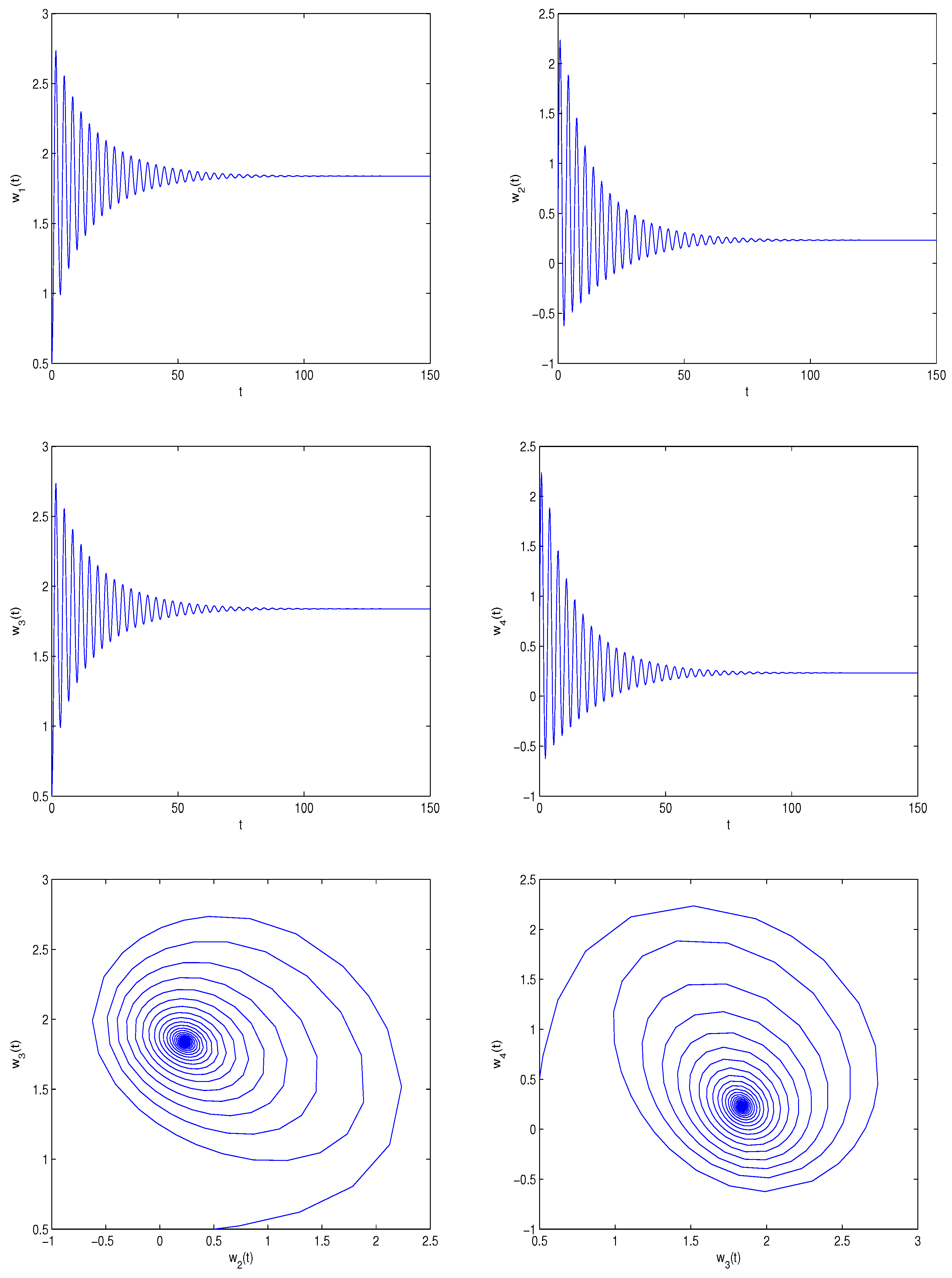
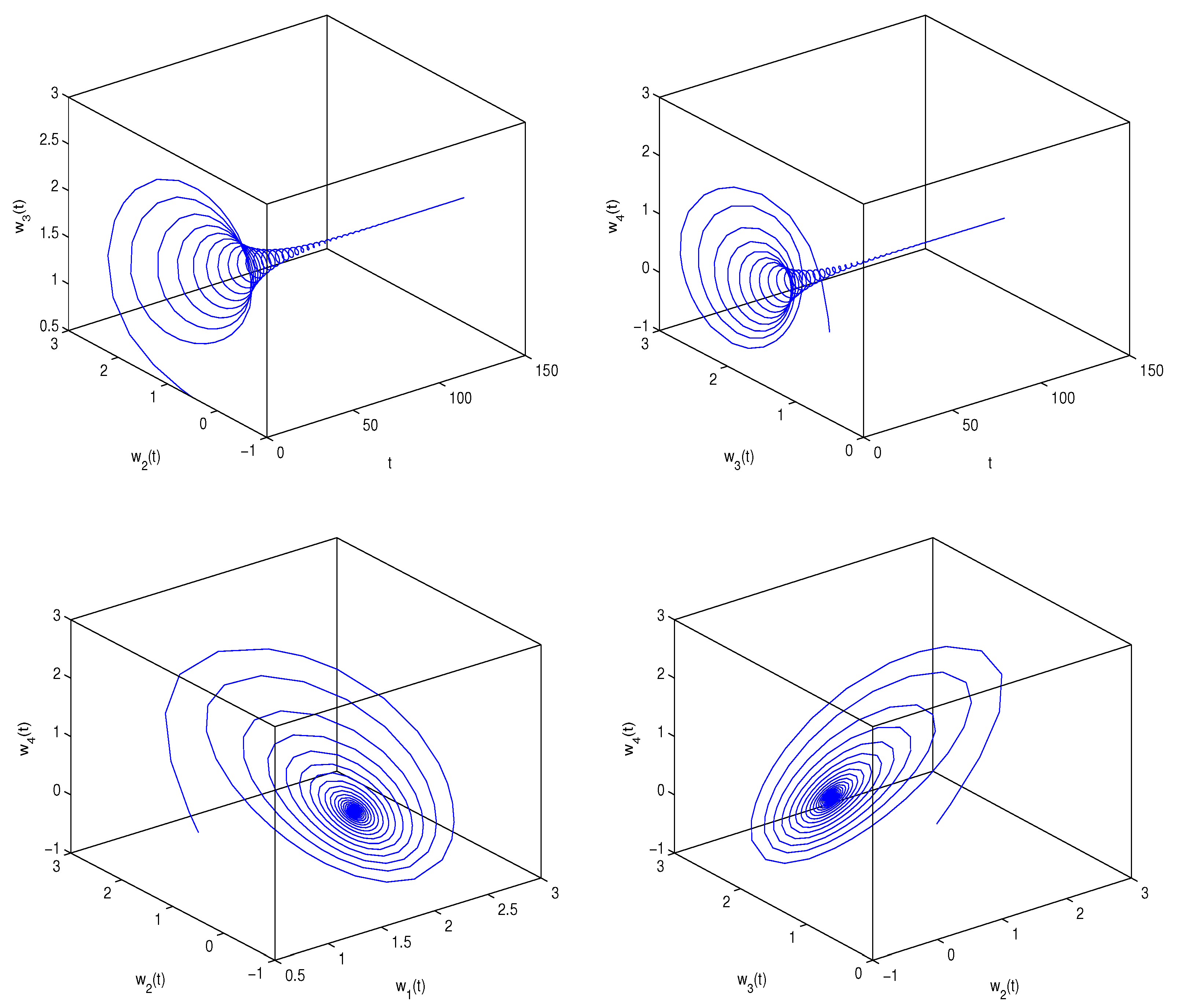
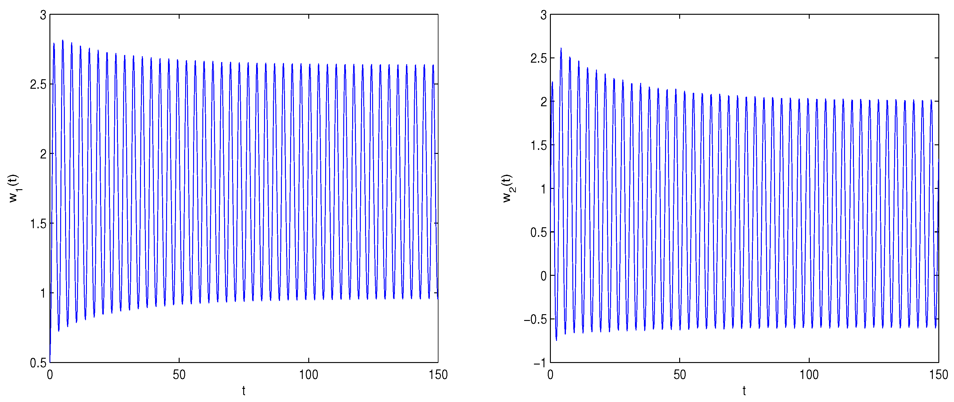
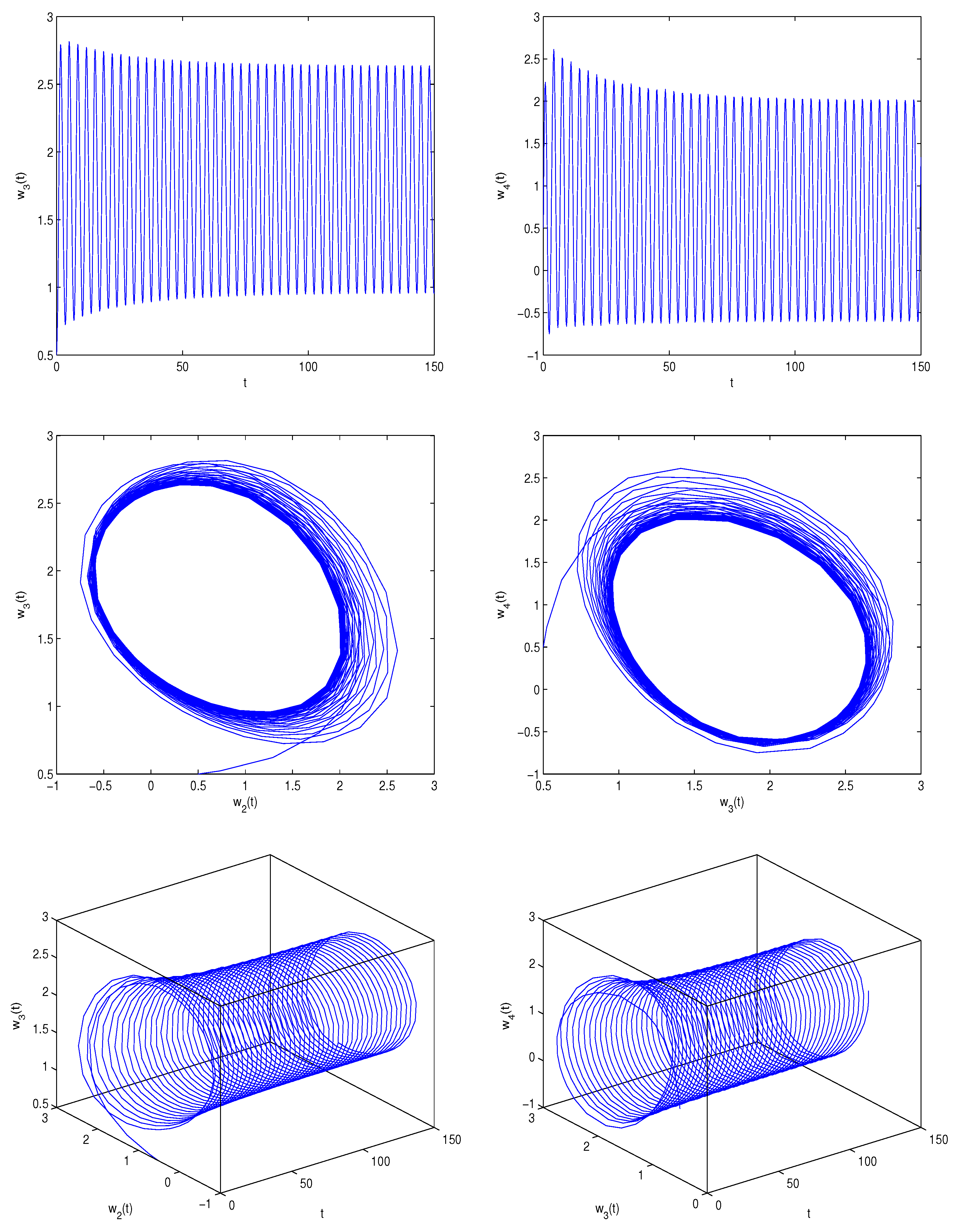
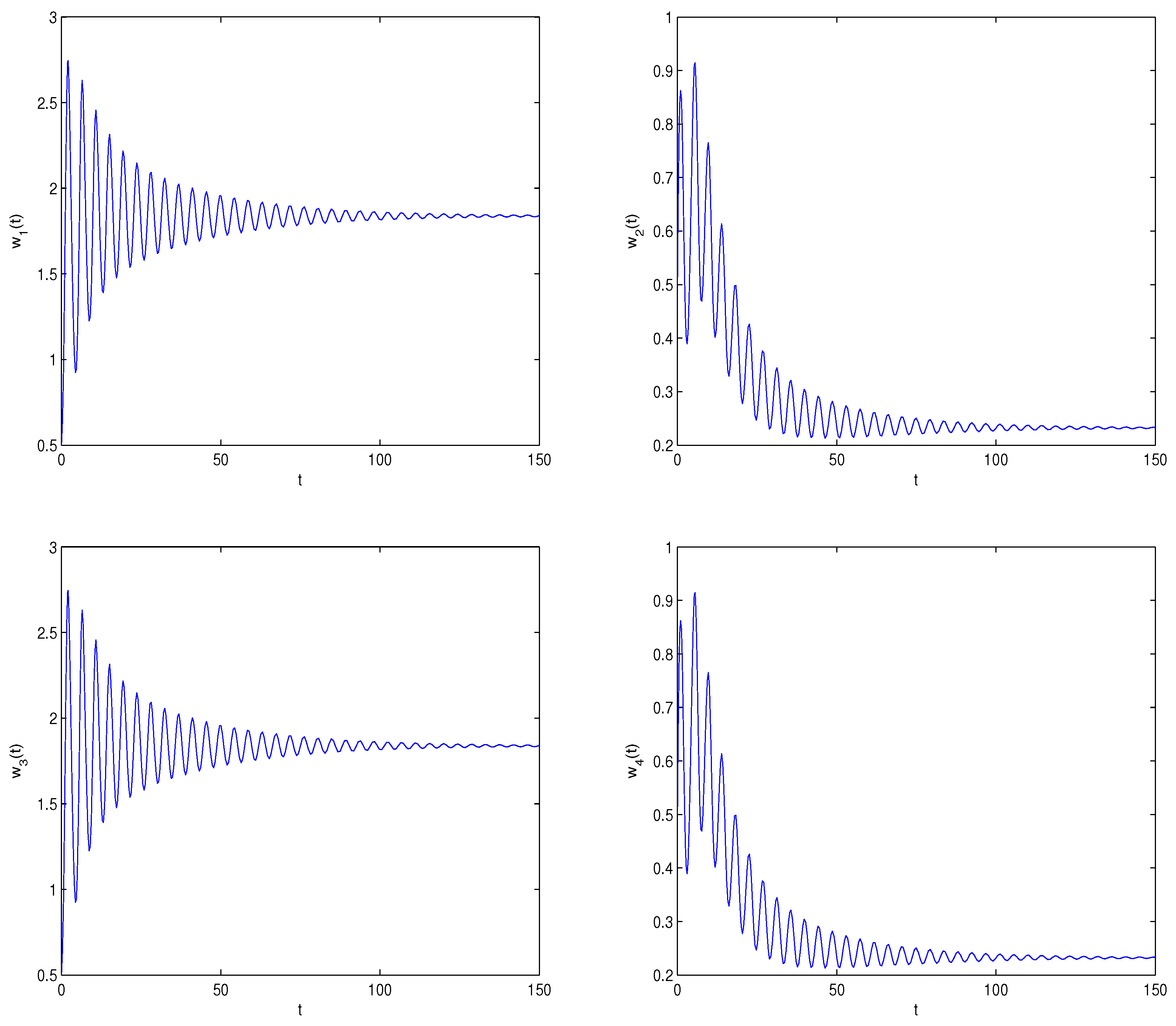
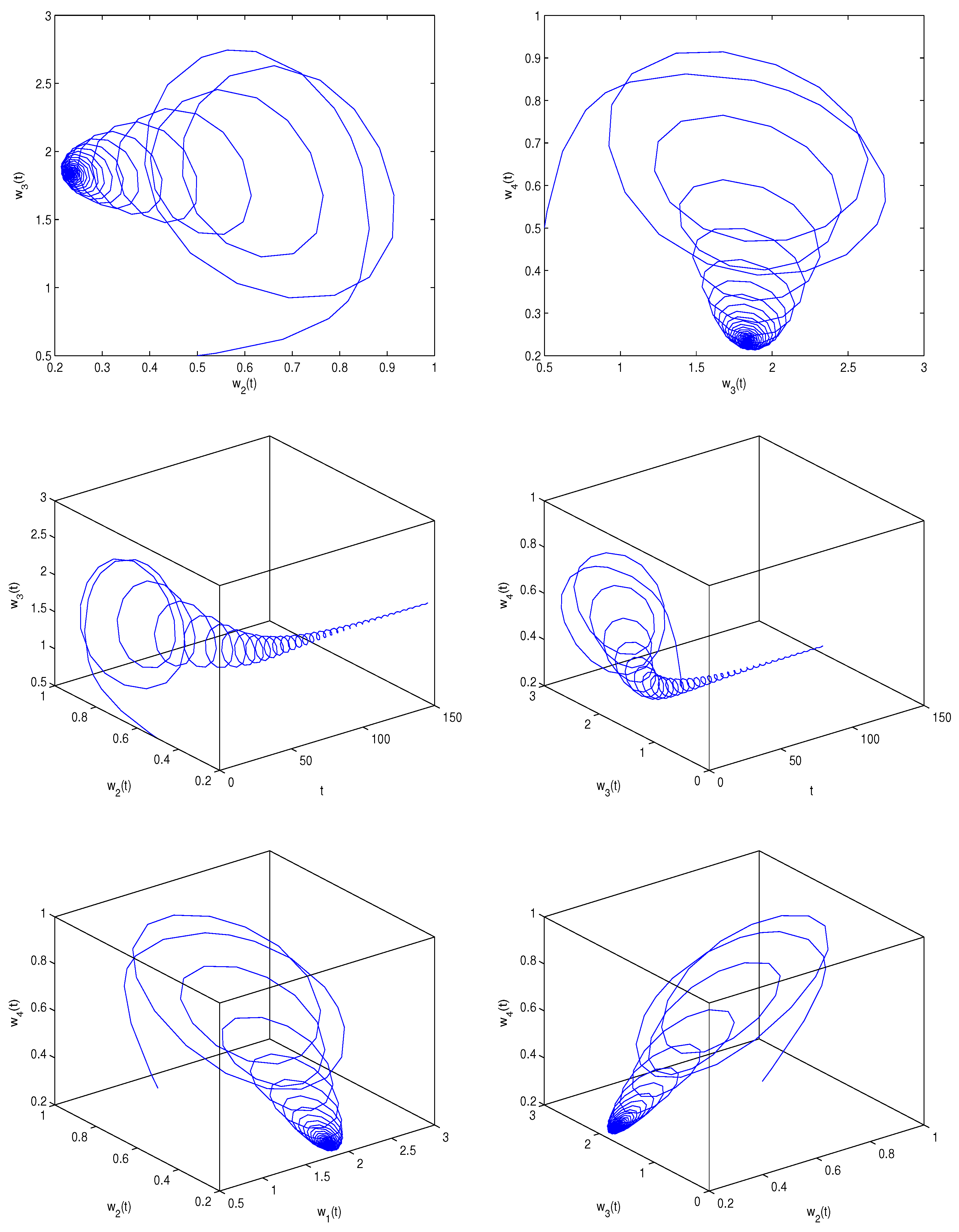
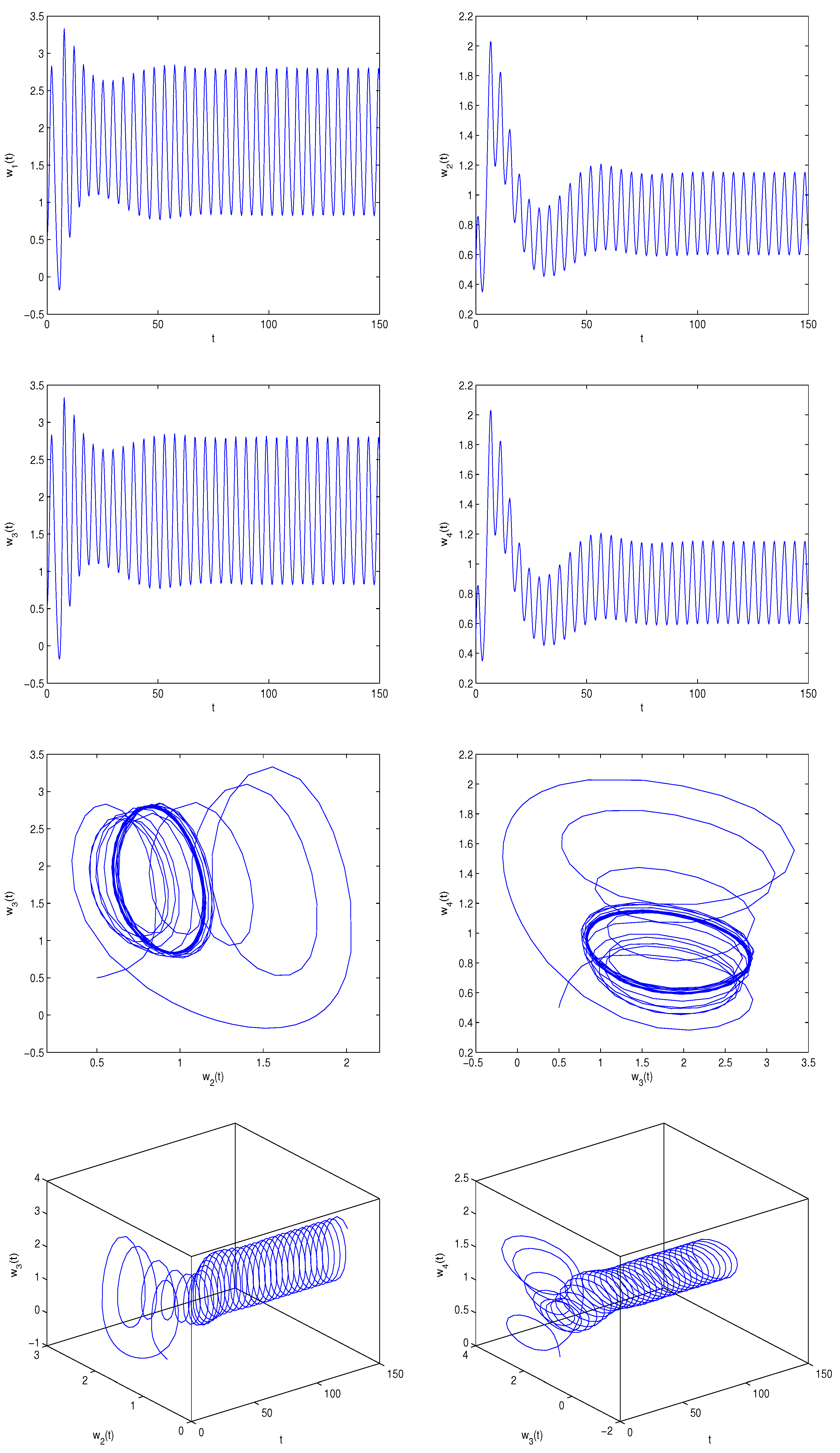
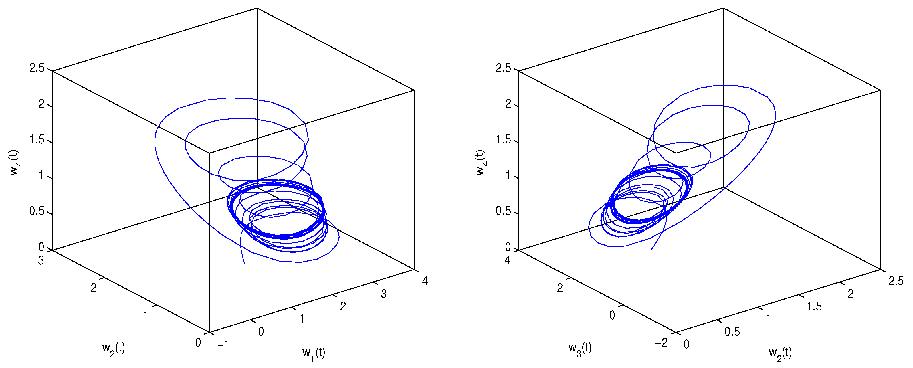
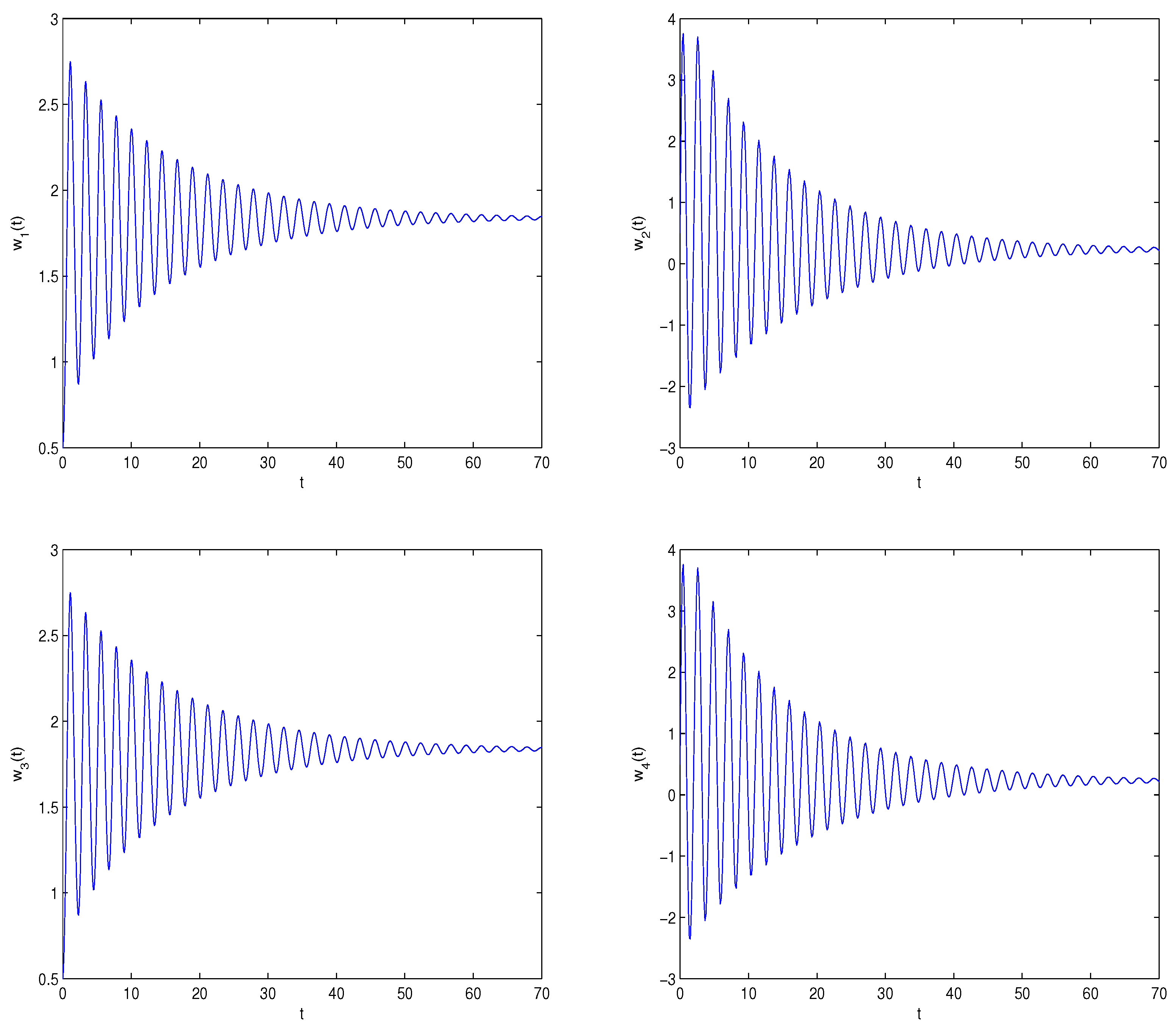
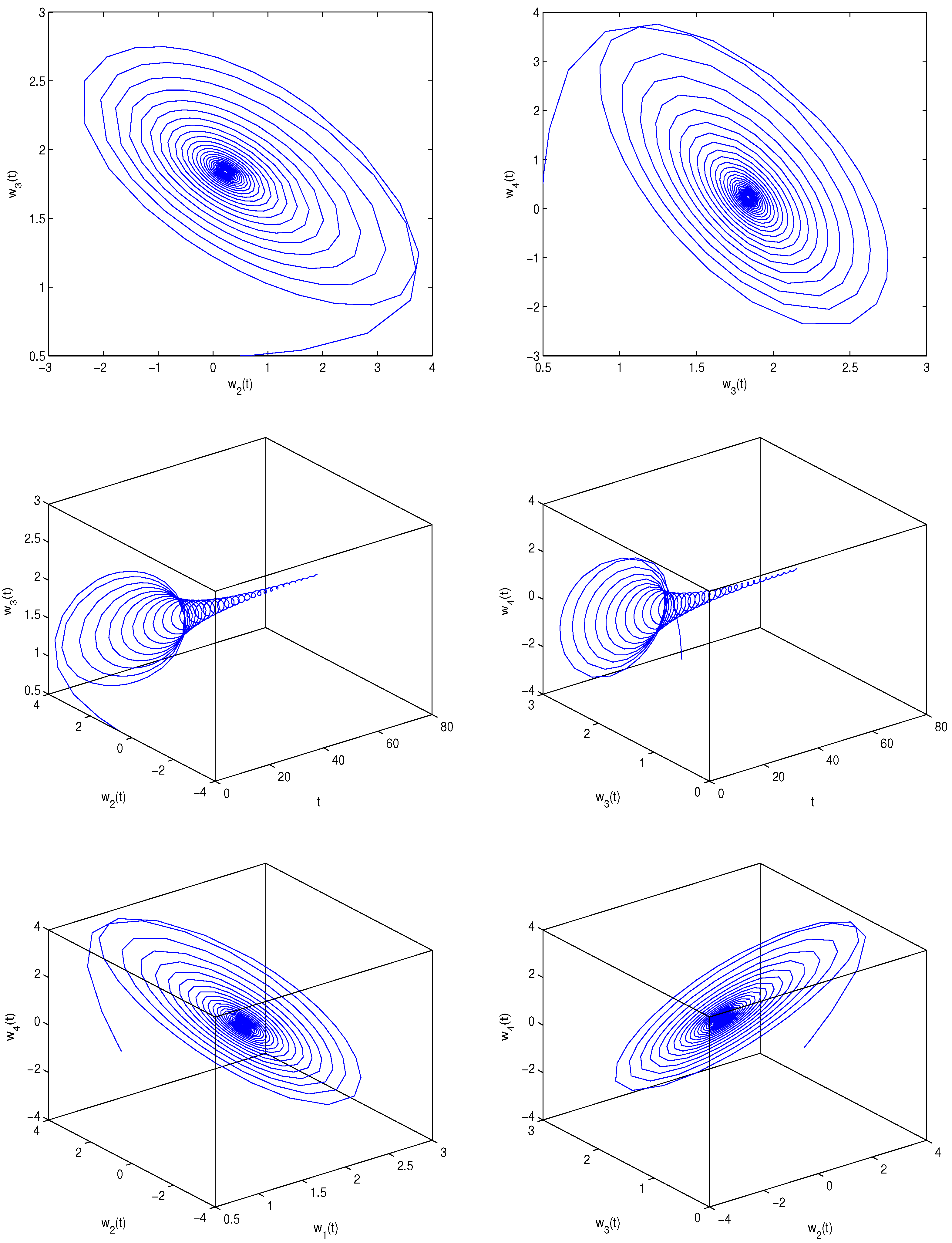
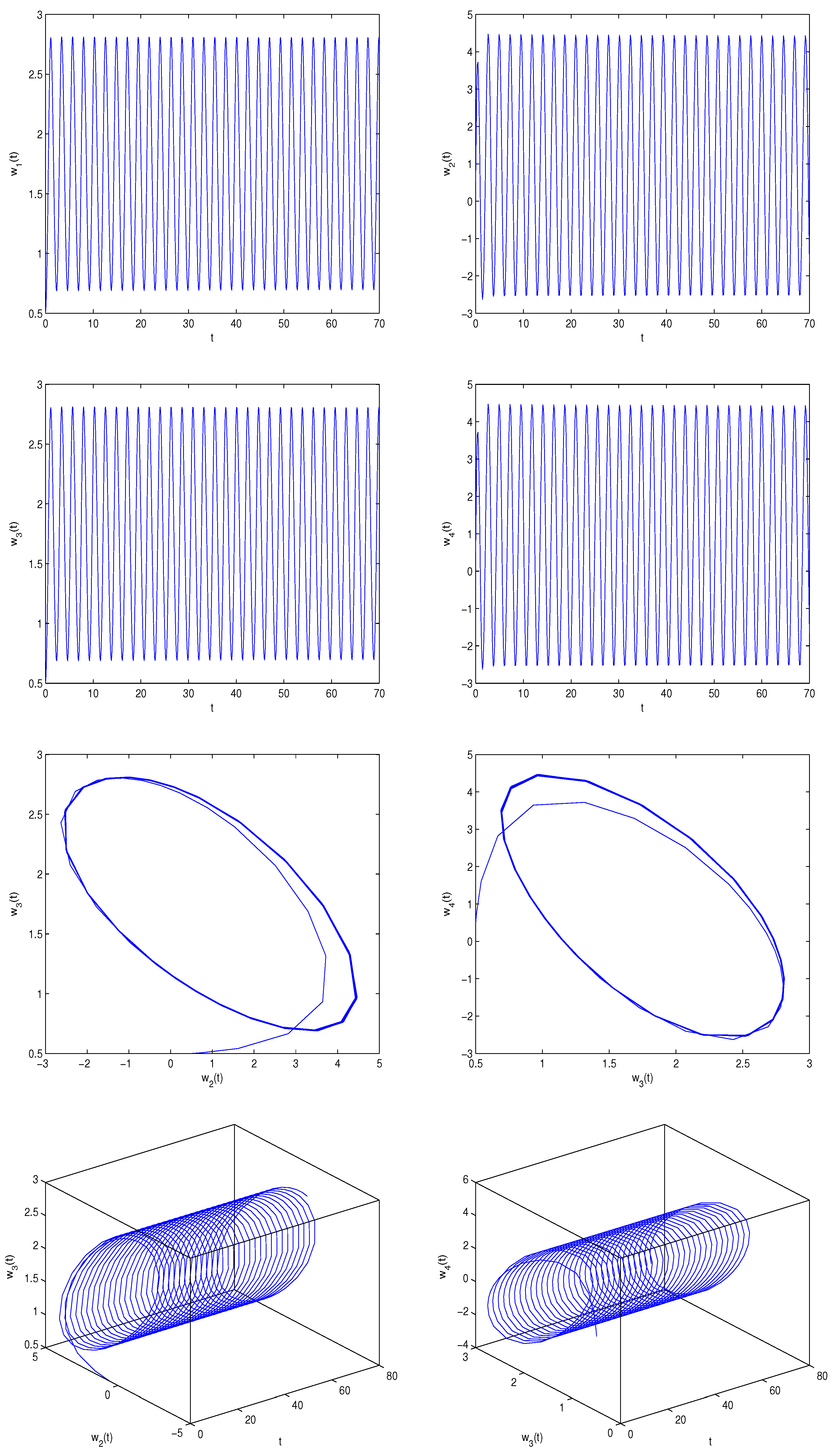
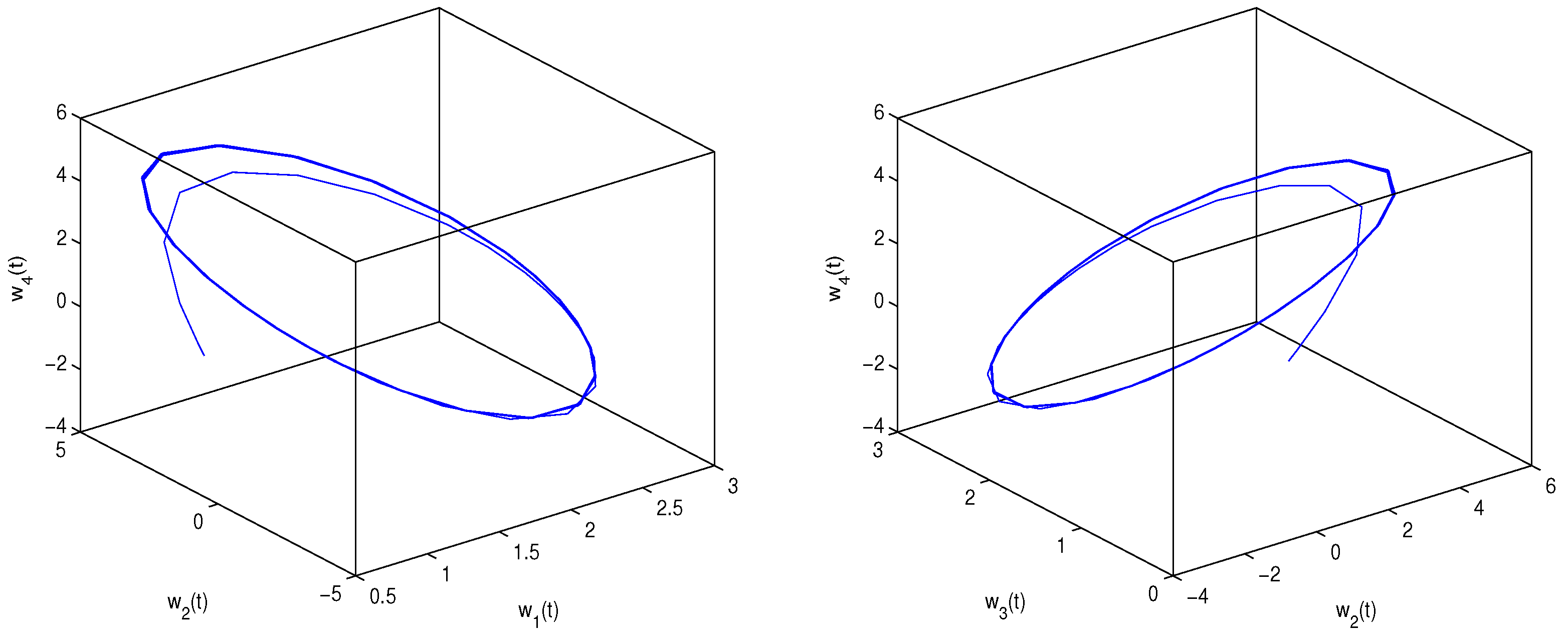
6. Simulation Outcomes

In this section, we use the standard Euler methods [47] to carry out numerical simulations.
Example 1. 
Consider the following FitzHugh–Nagumo neural model:
d w 1 0.91 ( t ) d t 0.91 = 0.33 w 2 + w 1 1 3 w 1 3 + 1.5 ( w 1 w 3 ( t θ ) ) , d w 2 0.91 ( t ) d t 0.91 = 1 0.33 ( w 1 1.88 + 0.18 w 2 ) , d w 3 0.91 ( t ) d t 0.91 = 0.33 w 4 + w 3 1 3 w 3 3 + 1.5 ( w 3 w 1 ( t θ ) ) , d w 4 0.91 ( t ) d t 0.91 = 1 0.33 ( w 3 1.88 + 0.18 w 4 ) .
One can lightly see that system (90) admits a unique positive equilibrium point W 0 ( w 1 , w 2 , w 3 , w 4 ) = W 0 ( 1.8382 , , 1.8382 , 0.2322 ) . Due to the Matlab software, one can lightly obtain ϕ 0 = 0.7499 and θ 0 = 0.62 . We can check that ( A 1 ) ( A 3 ) of Theorem 1 are satisfied. Thus, when θ [ 0 , 0.62 ) , then the positive equilibrium point W 0 ( 1.8382 , 0.2322 , 1.8382 , 0.2322 ) of system (90) remains locally asymptotically stable. Select θ = 0.6 < θ 0 = 0.62 . The simulation outcomes are presented in Figure 1. One can see from Figure 1 that if θ is less than the delay point θ 0 = 0.62 , then w 1 ( t ) 1.8382 , w 2 ( t ) 0.2322 , w 3 ( t ) 1.8382 , w 4 ( t ) 0.2322 , respectively, as t . When θ crosses the delay point θ 0 = 0.62 , then system (90) loses its stability and generates a cluster of periodic solutions (namely, Hopf bifurcations) at around W 0 ( 1.8382 , 0.2322 , 1.8382 , 0.2322 ) . Select θ = 0.635 . The simulation outcomes are presented in Figure 2. One can see from Figure 2 that ϑ is greater than the delay point θ 0 = 0.62 , then ( w 1 ( t ) , w 2 ( t ) , w 3 ( t ) , w 4 ( t ) ) is a periodic oscillatory state around W 0 ( 1.8382 , 0.2322 , 1.8382 , 0.2322 ) . To further illustrate the Hopf bifurcation situation, we present the corresponding bifurcation plots (see Figure 3, Figure 4, Figure 5 and Figure 6). Depending on Figure 3, Figure 4, Figure 5 and Figure 6, we can understand the relationship between θ- w 1 , θ- w 2 , θ- w 3 , θ- w 4 , respectively. Obviously, the bifurcation value of system (90) is 0.62 . Furthermore, the quantitative relation between ϕ 0 and θ 0 is provided via Table 1.
Remark 3. 
In order to achieve local asymptotic stability, we explore the characteristic equation of system (90) according to Section 3. In view of Theorem 1, we know the local asymptotic stability condition of system (90).
Remark 4. 
In the simulation, since 0 < q < 1 , we can choose the arbitrary q, which falls into the range of ( 0 , 1 ) . In this section, we choose q = 0.91 . Of course, we can choose ( 0.1 , 0.5 ) . For this case, we can also carry out the numerical simulations for this value for q ( 0.1 , 0.5 ) . Here, we omit it. But this does not affect the verification of Theorem 1.
Example 2. 
Consider the following fractional-order controlled FitzHugh–Nagumo neural model:
d 0.91 w 1 ( t ) d t 0.91 = 0.33 w 2 + w 1 1 3 w 1 3 + 1.5 ( w 1 w 3 ( t θ ) ) , d 0.91 w 2 ( t ) d t 0.91 = 1 0.33 ( w 1 1.88 + 0.18 w 2 ) + ρ p ( w 2 ( t ) w 2 ) + ρ d d 0.91 ( w 2 ( t ) w 2 ) d t 0.91 , d 0.91 w 3 ( t ) d t 0.91 = 0.33 w 4 + w 3 1 3 w 3 3 + 1.5 ( w 3 w 1 ( t θ ) ) , d 0.91 w 4 ( t ) d t 0.91 = 1 0.33 ( w 3 1.88 + 0.18 w 4 ) + ϱ p ( w 4 ( t ) w 4 ) + ϱ d d 0.91 ( w 4 ( t ) w 4 ) d t 0.91 .
One can lightly see that system (91) admits a unique positive equilibrium point W 0 ( w 1 , w 2 , w 3 , w 4 ) = W 0 ( 1.8382 , 1.8382 , 0.2322 ) . Set ρ p = 0.2 , ρ d = 0.8 . Due to the Matlab software, one can lightly obtain φ 0 = 0.6877 and θ = 0.76 . We can check that ( A 1 ) , ( A 4 ) , ( A 5 ) of Theorem 1 are satisfied. Thus, when θ [ 0 , 0.76 ) , then the positive equilibrium point W 0 ( 1.8382 , 0.2322 , 1.8382 , 0.2322 ) of system (91) remains locally asymptotically stable. Select θ = 0.75 < θ = 0.76 . The simulation outcomes are presented in Figure 7. One can see from Figure 7 that if θ is less than the delay point, θ = 0.76 , then w 1 ( t ) 1.8382 , w 2 ( t ) 0.2322 , w 3 ( t ) 1.8382 , w 4 ( t ) 0.2322 , respectively, as t . When θ crosses the delay point, θ = 0.76 , then system (91) loses its stability and generates a cluster of periodic solutions (namely, Hopf bifurcations) at around W 0 ( 1.8382 , 0.2322 , 1.8382 , 0.2322 ) . Select θ = 0.8 . The simulation outcomes are presented in Figure 8. One can see in Figure 8 that if ϑ is greater than the delay point, θ = 0.76 , then ( w 1 ( t ) , w 2 ( t ) , w 3 ( t ) , w 4 ( t ) ) remains a periodic oscillatory state around W 0 ( 1.8382 , 0.2322 ., 1.8382 , 0.2322 ) . To further illustrate the Hopf bifurcation situation, we present the corresponding bifurcation plots (see Figure 9, Figure 10, Figure 11 and Figure 12). Depending on Figure 9, Figure 10, Figure 11 and Figure 12, we can understand the relationship among θ- w 1 , θ- w 2 , θ- w 3 , and θ- w 4 , respectively. Obviously, the bifurcation value of system (91) is 0.76 . Furthermore, the quantitative relation between φ 0 and θ is presented in Table 2.
Example 3. 
Consider the following fractional-order controlled FitzHugh–Nagumo neural model:
d 0.91 w 1 ( t ) d t 0.91 = 0.33 w 2 + w 1 1 3 w 1 3 + 1.5 ( w 1 w 3 ( t θ ) ) , d 0.91 w 2 ( t ) d t 0.91 = κ 1 1 0.33 ( w 1 1.88 + 0.18 w 2 ) + κ 2 [ w 2 ( t θ ) w 2 ( t ) ] , d 0.91 w 3 ( t ) d t 0.91 = 0.33 w 4 + w 3 1 3 w 3 3 + 1.5 ( w 3 w 1 ( t θ ) ) , d 0.91 w 4 ( t ) d t 0.91 = κ 1 1 0.33 ( w 3 1.88 + 0.18 w 4 ) + κ 2 [ w 4 ( t θ ) w 4 ( t ) ] .
One can lightly see that system (92) admits a unique positive equilibrium point W 0 ( w 1 , w 2 , w 3 , w 4 ) = W 0 ( 1.8382 , , 1.8382 , 0.2322 ) . Set κ 1 = 4.2 , κ 2 = 0.2 . Due to the Matlab software, one can lightly obtain ϑ 0 = 0.2976 and θ = 0.46 . We can check that ( A 1 ) , ( A 6 ) , ( A 7 ) of Theorem 1 are satisfied. Thus, when θ [ 0 , 0.46 ) , then the positive equilibrium point W 0 ( 1.8382 , 0.2322 , 1.8382 , 0.2322 ) of system (92) remains locally asymptotically stable. Select θ = 0.45 < θ = 0.46 . The simulation outcomes are presented in Figure 13. One can find from Figure 13 that if θ is less than the delay point, θ = 0.46 , then w 1 ( t ) 1.8382 , w 2 ( t ) 0.2322 , w 3 ( t ) 1.8382 , w 4 ( t ) 0.2322 , respectively, as t . When θ crosses the delay point, θ = 0.46 , then system (92) loses its stability and generates a cluster of periodic solutions (namely, Hopf bifurcations) at around W 0 ( 1.8382 , 0.2322 , 1.8382 , 0.2322 ) . Select θ = 0.473 . The simulation outcomes are presented in Figure 14. One can find from Figure 14 that ϑ is greater than the delay point, θ = 0.46 , then ( w 1 ( t ) , w 2 ( t ) , w 3 ( t ) , w 4 ( t ) ) remains in a periodic oscillatory state at around W 0 ( 1.8382 , 0.2322 , 1.8382 , 0.2322 ) . To further illustrate the Hopf bifurcation situation, we present the corresponding bifurcation plots (see Figure 15, Figure 16, Figure 17 and Figure 18). Depending on Figure 15, Figure 16, Figure 17 and Figure 18, we can understand the relationship between θ- w 1 , θ- w 2 , θ- w 3 , and θ- w 4 , respectively. Obviously, the bifurcation value of system (92) is 0.46 . Furthermore, the quantitative relation between ϑ 0 and θ is presented in Table 3.
Remark 5. 
According to the simulation outcomes of Examples 1–3, we know that the bifurcation values of system (90), system (91), and system (92) are θ 0 = 0.62 , θ = 0.76 , a n d θ = 0.46 , respectively, which implies that (i) we can enlarge the stability domain and postpone the timing of bifurcation generation of the Hopf bifurcation of system (90) via the P D p controller and (ii) we can narrow the stability domain and advance the timing of bifurcation generation of the Hopf bifurcation of system (90) via the hybrid controller.

7. Conclusions

Depending on earlier studies, we formulate a novel fractional-order coupled FitzHugh–Nagumo neural model with delay. By analyzing the characteristic equation of the formulated fractional-order coupled FitzHugh–Nagumo neural model, we discuss the stability and Hopf bifurcation issue. A delay-independent criterion on stability and Hopf bifurcation for the considered coupled FitzHugh–Nagumo neural model is obtained. Due to the two effective controllers ( P D p controller and hybrid controller), the stability domain and the Hopf bifurcation onset time of the formulated fractional-order coupled FitzHugh–Nagumo neural model are successfully dominated. The influence of delay on the stability domain and the Hopf bifurcation onset time is displayed. The acquired theoretical outcomes of this study possess great theoretical value in operating and designing networks. By adjusting the control parameter and time delay, we can effectively control the stability domain and the time of bifurcation onset in neural networks. The control techniques can also be applied to control the stability and bifurcation behavior of other neural networks. In addition, we can control the stability domain and the bifurcation onset time in model (3) via other controllers. This will be explored in future work.

Author Contributions

Methodology, Y.Z. and C.X.; Software, C.X.; Validation, Y.Z. and C.X.; Formal analysis, Y.Z. and C.X.; Writing—original draft, Y.Z. and C.X.; Writing—review & editing, Y.Z. and C.X. All authors have read and agreed to the published version of the manuscript.

Funding

This work is supported by the National Natural Science Foundation of China (no. 12261015, no. 62062018), the Project of High-level Innovative Talents of Guizhou Province ([2016]5651), Guizhou Key Laboratory of Big Data Statistical Analysis (no. [2019]5103), Key Project of Hunan Education Department (17A181), University Science and Technology Top Talents Project of Guizhou Province (KY[2018]047), Foundation of Science and Technology of Guizhou Province ([2019]1051), Guizhou University of Finance and Economics (2018XZD01).

Data Availability Statement

No data were used to support this study.

Conflicts of Interest

The authors declare that they have no competing interests.

References

  1. Goetze, F.; Lai, P.Y. Dynamics of synaptically coupled FitzHugh-Nagumo neurons. Chin. J. Phys. 2022, 77, 1365–1380. [Google Scholar] [CrossRef]
  2. Hodgkin, A.L.; Huxley, A.F. A quantitative description of membrane current and its application to conduction and excitation in nerve. J. Physiol. 1952, 117, 500–544. [Google Scholar] [CrossRef] [PubMed]
  3. Morris, C.; Lecar, H. Voltage oscillations in the barnacle giant muscle fiber. Biophys. J. 1981, 35, 193–213. [Google Scholar] [CrossRef] [PubMed]
  4. Ermentrout, G.B.; Kopell, N. Parabolic bursting in an excitable system coupled with a slow oscillation. SIAM J. Appl. Math. 1986, 46, 233–253. [Google Scholar] [CrossRef]
  5. FitzHugh, R. Impulses and physiological states in theoretical models of nerve membrane. Biophys. J. 1961, 1, 445–466. [Google Scholar] [CrossRef] [PubMed]
  6. Touboul, J.; Brette, R. Spiking dynamics of bidimensional integrate-and-fire neurons. SIAM J. Appl. Dyn. Syst. 2009, 8, 1462–1506. [Google Scholar] [CrossRef]
  7. Ermentrout, B. Type I membranes, phase resetting curves, and synchrony. Neural Comput. 1996, 8, 979–1001. [Google Scholar] [CrossRef]
  8. Zeng, C.H.; Zeng, C.P.; Gong, A.L.; Nie, L.R. Effect of time delay in FitzHugh-Nagumo neural model with correlations between multiplicative and additive noises. Physica A 2010, 389, 5117–5127. [Google Scholar] [CrossRef]
  9. Demina, M.V.; Kudryashov, N.A. Meromorphic solutions in the FitzHugh-Nagumo model. Appl. Math. Lett. 2018, 82, 18–23. [Google Scholar] [CrossRef]
  10. He, Z.L.; Li, C.D.; Chen, L.; Cao, Z.R. Dynamic behaviors of the FitzHugh-Nagumo neuron model with state-dependent impulsive effects. Neural Netw. 2020, 121, 497–511. [Google Scholar] [CrossRef]
  11. Zheng, Q.Q.; Shen, J.W. Turing instability induced by random network in FitzHugh-Nagumo model. Appl. Math. Comput. 2020, 381, 125304. [Google Scholar] [CrossRef]
  12. Gani, M.O.; Ogawa, T. Instability of periodic traveling wave solutions in a modified FitzHugh-Nagumo model for excitable media. Appl. Math. Comput. 2015, 256, 968–984. [Google Scholar] [CrossRef]
  13. Buckwar, E.; Samson, A.; Tamborrino, M.; Tubikanec, I. A splitting method for SDEs with locally Lipschitz drift: Illustration on the FitzHugh-Nagumo model. Appl. Numer. Math. 2022, 179, 191–220. [Google Scholar] [CrossRef]
  14. Chen, L.; Campbell, S.A. Hysteresis bifurcation and application to delayed FitzHugh-Nagumo neural systems. J. Math. Anal. Appl. 2021, 500, 125151. [Google Scholar] [CrossRef]
  15. Ciszak, M.; Balle, S.; Piro, O.; Marino, F. Intermittent chaotic spiking in the van der Pol-FitzHugh-Nagumo system with inertia. Chaos Solitons Fractals 2023, 167, 113053. [Google Scholar] [CrossRef]
  16. Njitacke, Z.T.; Takembo, C.N.; Awrejcewicz, J.; Fouda, H.P.E.; Kengne, J. Hamilton energy, complex dynamical analysis and information patterns of a new memristive FitzHugh-Nagumo neural network. Chaos Solitons Fractals 2022, 160, 112211. [Google Scholar] [CrossRef]
  17. Achouri, H.; Aouiti, C.; Hamed, B.B. Codimension two bifurcation in a coupled FitzHugh-Nagumo system with multiple delays. Chaos Solitons Fractals 2022, 156, 111824. [Google Scholar] [CrossRef]
  18. Hoff, A.; Santos, J.V.d.; Manchein, C.; Albuquerque, H.A. Numerical bifurcation analysis of two coupled FitzHugh-Nagumo oscillators. Eur. Phys. J. 2014, 87, 87–151. [Google Scholar] [CrossRef]
  19. Gan, C.B.; Perc, M.; Wang, Q.Y. Delay-aided stochastic multiresonances on scale-free FitzHugh Nagumo neuronal networks. Chin. Phys. 2010, 19, 040508. [Google Scholar]
  20. Jia, J.Y.; Liu, H.H.; Xu, C.L.; Yan, F. Dynamic effects of time delay on a coupled FitzHugh-Nagumo neural system. Alex. Eng. J. 2015, 54, 241–250. [Google Scholar] [CrossRef]
  21. Petras, I. Fractional-Order Nonlinear Systems; Springer: London, UK, 2011. [Google Scholar]
  22. Xu, C.J.; Liao, M.X.; Li, P.L.; Guo, Y.; Liu, Z.X. Bifurcation properties for fractional order delayed BAM neural networks. Cogn. Comput. 2021, 13, 322–356. [Google Scholar] [CrossRef]
  23. Xu, C.J.; Mu, D.; Liu, Z.X.; Pang, Y.C.; Liao, M.X.; Li, P.L.; Yao, L.Y.; Qin, Q.W. Comparative exploration on bifurcation behavior for integer-order and fractional-order delayed BAM neural networks. Nonlinear Anal. Model. Control 2022, 27, 1030–1053. [Google Scholar] [CrossRef]
  24. Li, P.L.; Gao, R.; Xu, C.J.; Shen, J.W.; Ahmad, S.; Li, Y. Exploring the impact of delay on Hopf bifurcation of a type of BAM neural network models concerning three nonidentical delays. Neural Process. Lett. 2023, 55, 5905–5921. [Google Scholar] [CrossRef]
  25. Xu, C.J.; Zhao, Y.Y.; Lin, J.T.; Pang, Y.C.; Liu, Z.X.; Shen, J.W.; Qin, Y.X.; Farman, M.; Ahmad, S. Mathematical exploration on control of bifurcation for a plankton-oxygen dynamical model owning delay. J. Math. Chem. 2023. [Google Scholar] [CrossRef]
  26. Ou, W.; Xu, C.J.; Cui, Q.Y.; Pang, Y.C.; Liu, Z.X.; Shen, J.W.; Baber, M.Z.; Farman, M.; Ahmad, S. Hopf bifurcation exploration and control technique in a predator-prey system incorporating delay. Aims Math. 2023, 9, 1622–1651. [Google Scholar] [CrossRef]
  27. Cui, C.Q.; Xu, C.J.; Ou, W.; Pang, Y.C.; Liu, Z.X.; Li, P.L.; Yao, L.Y. Bifurcation behavior and hybrid controller design of a 2D Lotka-Volterra commensal symbiosis system accompanying delay. Mathematics 2023, 11, 4808. [Google Scholar] [CrossRef]
  28. Maharajan, C.; Sowmiya, C.; Xu, C.J. Fractional order uncertain BAM neural networks with mixed time delays: An existence and Quasi-uniform stability analysis. J. Intell. Fuzzy Syst. 2023, 46, 4291–4313. [Google Scholar] [CrossRef]
  29. Xiao, J.Y.; Wen, S.P.; Yang, X.J.; Zhong, S.M. New approach to global Mittag-Leffler synchronization problem of fractional-order quaternion-valued BAM neural networks based on a new inequality. Neural Netw. 2020, 122, 320–337. [Google Scholar] [CrossRef]
  30. Xu, C.J.; Rahman, M.; Baleanu, D. On fractional-order symmetric oscillator with offset-boosting control. Nonlinear Anal. Control 2022, 27, 994–1008. [Google Scholar] [CrossRef]
  31. Li, N.; Yan, M.T. Bifurcation control of a delayed fractional-order prey-predator model with cannibalism and disease. Phys. Stat. Mech. Its Appl. 2022, 600, 127600. [Google Scholar] [CrossRef]
  32. Kao, Y.G.; Li, H. Asymptotic multistability and local S-asymptotic ω-periodicity for the nonautonomous fractional-order neural networks with impulses. Sci. China Inf. Sci. 2021, 64, 112207. [Google Scholar] [CrossRef]
  33. Luo, R.Z.; Liu, S.; Song, Z.J.; Zhang, F. Fixed-time control of a class of fractional-order chaotic systems via backstepping method. Chaos Solitons Fractals 2023, 167, 113076. [Google Scholar] [CrossRef]
  34. Jin, X.C.; Lu, J.G.; Zhang, Q.H. Delay-dependent and order-dependent conditions for stability and stabilization of fractional-order memristive neural networks with time-varying delays. Neurocomputing 2023, 522, 53–63. [Google Scholar] [CrossRef]
  35. Hao, Y.J.; Zhang, M.H.; Cui, Y.H.; Cheng, G.; Xie, J.Q.; Chen, Y.M. Dynamic analysis of variable fractional order cantilever beam based on shifted Legendre polynomials algorithm. J. Comput. Appl. Math. 2023, 423, 114952. [Google Scholar] [CrossRef]
  36. Hioual, A.; Ouannas, A.; Grassi, G.; Oussaeif, T.E. Nonlinear nabla variable-order fractional discrete systems: Asymptotic stability and application to neural networks. J. Comput. Appl. Math. 2023, 423, 114939. [Google Scholar] [CrossRef]
  37. Huang, C.D.; Nie, X.B.; Zhao, X.; Song, Q.K.; Tu, Z.W.; Xiao, M.; Cao, J.D. Novel bifurcation results for a delayed fractional-order quaternion-valued neural network. Neural Netw. 2019, 117, 67–93. [Google Scholar] [CrossRef] [PubMed]
  38. Ali, M.S.; Narayanan, G.; Sevgen, S.; Shekher, V.; Arik, S. Global stability analysis of fractional-order fuzzy BAM neural networks with time delay and impulsive effects. Commun. Nonlinear Sci. Numer. Simul. 2019, 78, 104853. [Google Scholar]
  39. Arslan, E.; Narayanan, G.; Ali, M.S.; Arik, S.; Saroha, S. Controller design for finite-time and fixed-time stabilization of fractional-order memristive complex-valued BAM neural networks with uncertain parameters and time-varying delays. Neural Networks 2020, 130, 60–74. [Google Scholar] [CrossRef] [PubMed]
  40. Amine, S.; Hajri, Y.; Allali, K. A delayed fractional-order tumor virotherapy model: Stability and Hopf bifurcation. Chaos Solitons Fractals 2022, 161, 112396. [Google Scholar] [CrossRef]
  41. Xu, C.J.; Mu, D.; Liu, Z.X.; Pang, Y.C.; Liao, M.X.; Aouiti, C. New insight into bifurcation of fractional-order 4D neural networks incorporating two different time delays. Commun. Nonlinear Sci. Numer. Simul. 2023, 118, 107043. [Google Scholar] [CrossRef]
  42. Huang, C.D.; Cao, J.D.; Xiao, M.; Alsaedi, A.; Hayat, T. Effects of time delays on stability and Hopf bifurcation in a fractional ring-structured network with arbitrary neurons. Commun. Nonlinear Sci. Numer. Simul. 2018, 57, 1–13. [Google Scholar] [CrossRef]
  43. Alidousti, J. Stability and bifurcation analysis for a fractional prey-predator scavenger model. Appl. Math. Model. 2020, 81, 342–355. [Google Scholar] [CrossRef]
  44. Xu, C.J.; Liao, M.X.; Li, P.L.; Yao, L.Y.; Qin, Q.W.; Shang, Y.L. Chaos control for a fractional-order Jerk system via time delay feedback controller and mixed controller. Fractal Fract. 2021, 5, 257. [Google Scholar] [CrossRef]
  45. Eshaghi, S.; Ghaziani, R.K.; Ansari, A. Hopf bifurcation, chaos control and synchronization of a chaotic fractional-order system with chaos entanglement function. Math. Comput. Simul. 2020, 172, 321–340. [Google Scholar] [CrossRef]
  46. Zhao, L.Z.; Huang, C.D.; Cao, J.D. Effects of double delays on bifurcation for a fractional-order neural network. Cogn. Neurodyn. 2022, 16, 1189–1201. [Google Scholar] [CrossRef] [PubMed]
  47. Fleitas, A.; Méndez, J.A.; Nápoles, J.E.; Sigarreta, J.M. On fractional Lienard-type systems. Rev. Mex. Física 2019, 65, 618–625. [Google Scholar] [CrossRef]
  48. Tang, Y.H.; Xiao, M.; Jiang, G.P.; Lin, J.X.; Cao, J.D.; Zheng, W.X. Fractional-order PD control at Hopf bifurcations in a fractional-ordr congestion control system. Nonlinear Dyn. 2007, 90, 2185–2198. [Google Scholar] [CrossRef]
  49. Ding, D.W.; Zhang, X.Y.; Cao, J.D.; Wang, N.A.; Liang, D. Bifurcation control of complex networks model via PD controller. Neurocomputing 2016, 175, 1–9. [Google Scholar] [CrossRef]
  50. Huang, C.D.; Mo, S.S.; Cao, J.D. Detections of bifurcation in a fractional-order Cohen-Grossberg neural network with multiple delays. Cogn. Neurodyn. 2023, 1–18. [Google Scholar] [CrossRef]
  51. Podlubny, I. Fractional Differential Equations; Academic Press: New York, NY, USA, 1999. [Google Scholar]
  52. Bandyopadhyay, B.; Kamal, S. Stabliization and Control of Fractional Order Systems: A Sliding Mode Approach; Springer: Heidelberg, Germany, 2015; Volume 317. [Google Scholar]
  53. Matignon, D. Stability results for fractional differential equations with applications to control processing. Comput. Eng. Syst. Appl. 1996, 2, 963–968. [Google Scholar]
  54. Wang, X.H.; Wang, Z.; Xia, J.W. Stability and bifurcation control of a delayed fractional-order eco-epidemiological model with incommensurate orders. J. Frankl. Inst. 2019, 356, 8278–8295. [Google Scholar] [CrossRef]
  55. Deng, W.H.; Li, C.P.; Lü, J.H. Stability analysis of linear fractional differential system with multiple time delays. Nonlinear Dyn. 2007, 48, 409–416. [Google Scholar] [CrossRef]
  56. Zhang, Z.Z.; Yang, H.Z. Hybrid control of Hopf bifurcation in a two prey one predator system with time delay. In Proceedings of the 33rd Chinese Control Conference, Nanjing, China, 28–30 July 2014; pp. 6895–6900. [Google Scholar]
  57. Zhang, L.P.; Wang, H.N.; Xu, M. Hybrid control of bifurcation in a predator-prey system with three delays. Acta Phys. Sin. 2011, 60, 010506. [Google Scholar] [CrossRef]
Figure 1. Simulation outcomes of system (90) involving θ = 0.6 < θ 0 = 0.62 . The positive equilibrium point W 0 ( 1.8382 , 0.2322 , 1.8382 , 0.2322 ) of system (90) remains locally asymptotically stable.
Fractalfract 08 00229 g001aFractalfract 08 00229 g001b
Figure 2. Simulation outcomes of system (90) involving θ = 0.635 > θ 0 = 0.62 . show that System (90) generates a cluster of periodic solutions (namely, Hopf bifurcations) at around the positive equilibrium point W 0 ( 1.8382 , 0.2322 , 1.8382 , 0.2322 ) .
Fractalfract 08 00229 g002aFractalfract 08 00229 g002bFractalfract 08 00229 g002c
Figure 3. Bifurcation figure of system (90): The delay, θ , versus the variable, w 1 . The bifurcation value is θ 0 = 0.62 .
Fractalfract 08 00229 g003
Figure 4. Bifurcation figure of system (90): The delay, θ , versus the variable, w 2 . The bifurcation value is θ 0 = 0.62 .
Fractalfract 08 00229 g004
Figure 5. Bifurcation figure of system (90): The delay, θ , versus the variable, w 3 . The bifurcation value is θ 0 = 0.62 .
Fractalfract 08 00229 g005
Figure 6. Bifurcation figure of system (90): The delay, θ , versus the variable, w 4 . The bifurcation value is θ 0 = 0.62 .
Fractalfract 08 00229 g006
Figure 7. Simulation outcomes of system (91) involving θ = 0.75 < θ = 0.76 . The positive equilibrium point W 0 ( 1.8382 , 0.2322 , 1.8382 , 0.2322 ) of system (91) remains locally asymptotically stable.
Fractalfract 08 00229 g007aFractalfract 08 00229 g007b
Figure 8. Simulation outcomes of system (91) involving θ = 0.8 > θ = 0.76 . : System (90) generates a cluster of periodic solutions (namely, Hopf bifurcations) at around the positive equilibrium point W 0 ( 1.8382 , 0.2322 , 1.8382 , 0.2322 ) .
Fractalfract 08 00229 g008aFractalfract 08 00229 g008b
Figure 9. Bifurcation figure of system (91): The delay, θ , versus the variable, w 1 . The bifurcation value is θ = 0.76 .
Fractalfract 08 00229 g009
Figure 10. Bifurcation figure of system (91): The delay, θ , versus the variable, w 2 . The bifurcation value is θ = 0.76 .
Fractalfract 08 00229 g010
Figure 11. Bifurcation figure of system (91): The delay, θ , versus the variable, w 3 . The bifurcation value is θ = 0.76 .
Fractalfract 08 00229 g011
Figure 12. Bifurcation figure of system (91): The delay, θ , versus the variable, w 4 . The bifurcation value is θ = 0.76 .
Fractalfract 08 00229 g012
Figure 13. Simulation outcomes of system (92) involving θ = 0.45 < θ = 0.46 . The positive equilibrium point W 0 ( 1.8382 , 0.2322 , 1.8382 , 0.2322 ) of system (92) remains locally asymptotically stable.
Fractalfract 08 00229 g013aFractalfract 08 00229 g013b
Figure 14. Simulation outcomes of system (92) involving θ = 0.473 > θ = 0.46 . : System (92) generates a cluster of periodic solutions (namely, Hopf bifurcations) at around the positive equilibrium point W 0 ( 1.8382 , 0.2322 , 1.8382 , 0.2322 ) .
Fractalfract 08 00229 g014aFractalfract 08 00229 g014b
Figure 15. Bifurcation figure of system (92): The delay, θ , versus the variable, w 1 . The bifurcation value is θ = 0.46 .
Fractalfract 08 00229 g015
Figure 16. Bifurcation figure of system (92): The delay, θ , versus the variable, w 2 . The bifurcation value is θ = 0.46 .
Fractalfract 08 00229 g016
Figure 17. Bifurcation figure of system (92): The delay, θ , versus the variable, w 3 . The bifurcation value is θ = 0.46 .
Fractalfract 08 00229 g017
Figure 18. Bifurcation figure of system (92): The delay, θ , versus the variable, w 4 . The bifurcation value is θ = 0.46 .
Fractalfract 08 00229 g018
Table 1. The quantitative relation between ϕ 0 and θ 0 of system (90).
ϕ 0 θ 0
0.1805 0.1231
0.3488 0.2519
0.4602 0.3452
0.6169 0.4879
0.6324 0.5027
0.7499 0.6200
0.8753 0.7543
0.9402 0.8276
1.0220 0.9238
Table 2. The quantitative relation between φ 0 and θ of system (91).
φ 0 θ
0.2103 0.1789
0.2790 0.2467
0.3383 0.3092
0.4566 0.4456
0.0993   0.5672
0.6089 0.6453
0.6877 0.7600
0.7268 0.8199
0.8112 0.9562
Table 3. The quantitative relation between ϑ 0 and θ of system (92).
ϑ 0 θ
0.1071 0.1542
0.1879 0.2789
0.2358 0.3563
0.2976 0.4600
0.3525 0.5562
0.3934 0.6303
0.4482 0.7328
0.5092 0.8513
0.5496 0.9327
Disclaimer/Publisher’s Note: The statements, opinions and data contained in all publications are solely those of the individual author(s) and contributor(s) and not of MDPI and/or the editor(s). MDPI and/or the editor(s) disclaim responsibility for any injury to people or property resulting from any ideas, methods, instructions or products referred to in the content.

