


A Low Power Analog Integrated Fractional Order Type-2 Fuzzy PID Controller


 ,
, 

Abstract
1. Introduction
- The low-power performance, operating in subthreshold regime.
- The pure analog implementation of a PID controller that combines both Fuzzy logic and fractional calculus to control the plant system.
2. Background
2.1. Literature Review
2.2. Fractional PID Control
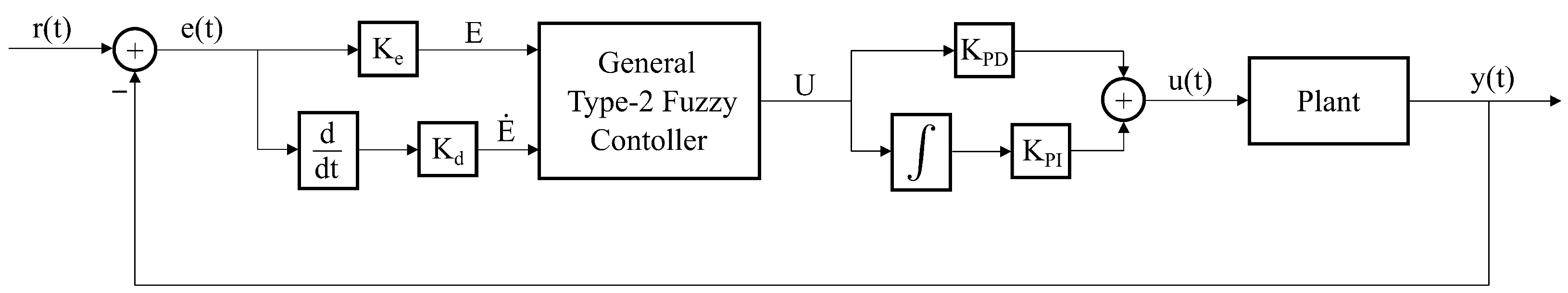
2.3. Type-2 Fuzzy PID Control
3. Proposed Design Methodology
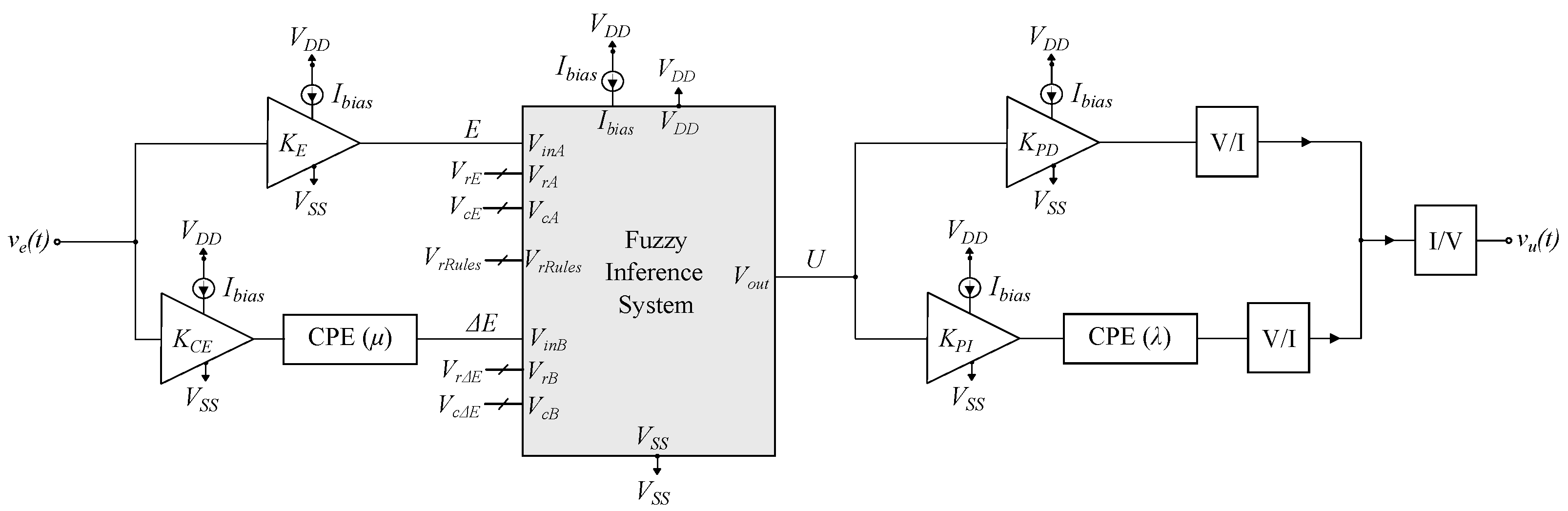
4. Circuit Implementation
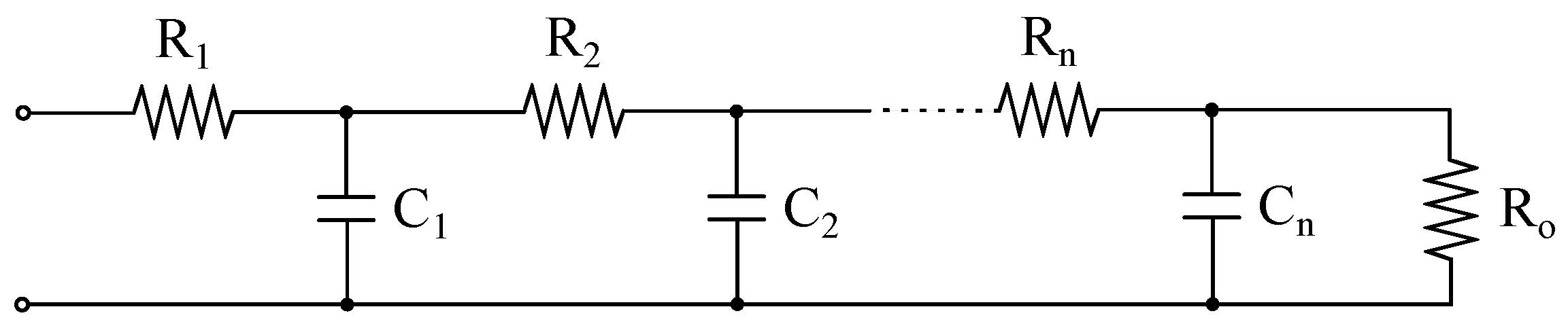
4.1. Fractional Order Circuits
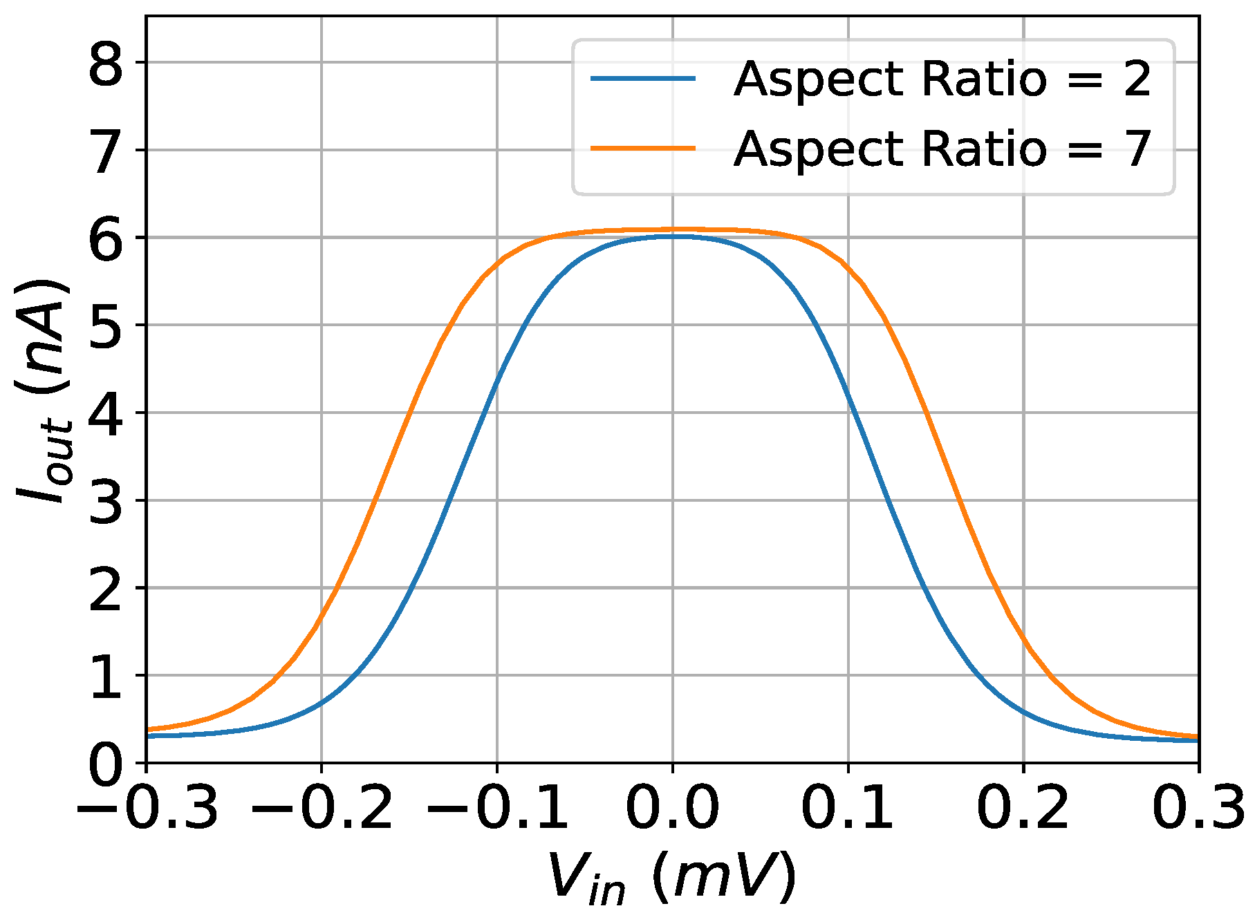
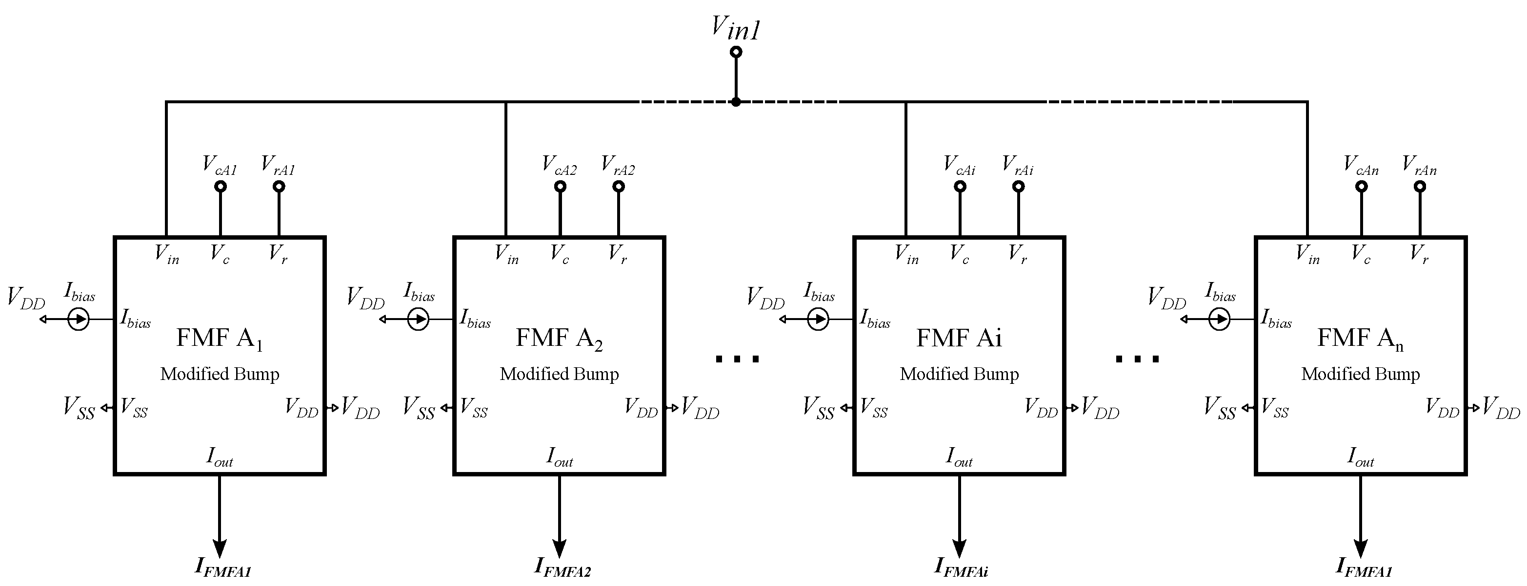
4.2. Gaussian Function Circuit
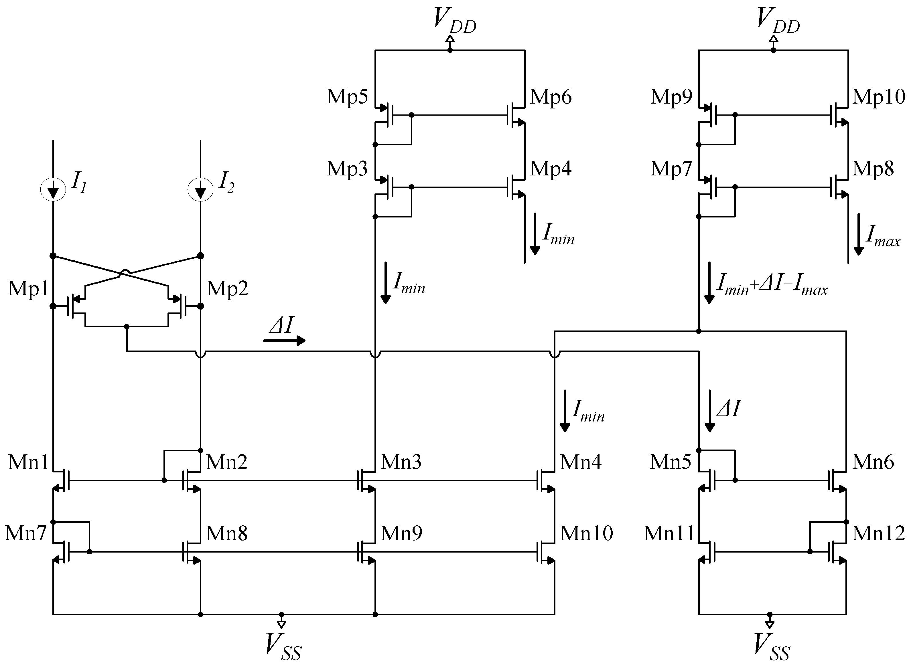
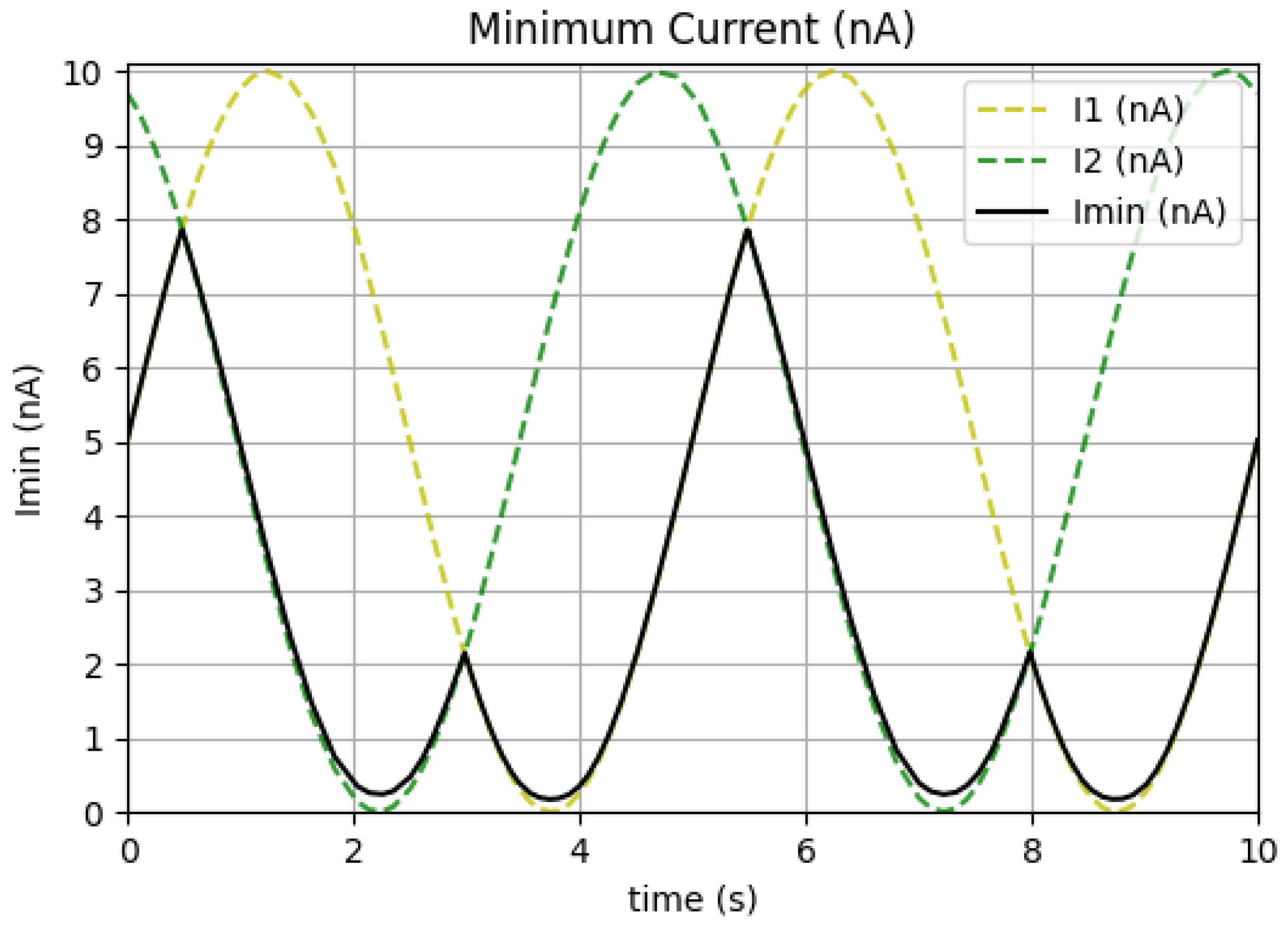
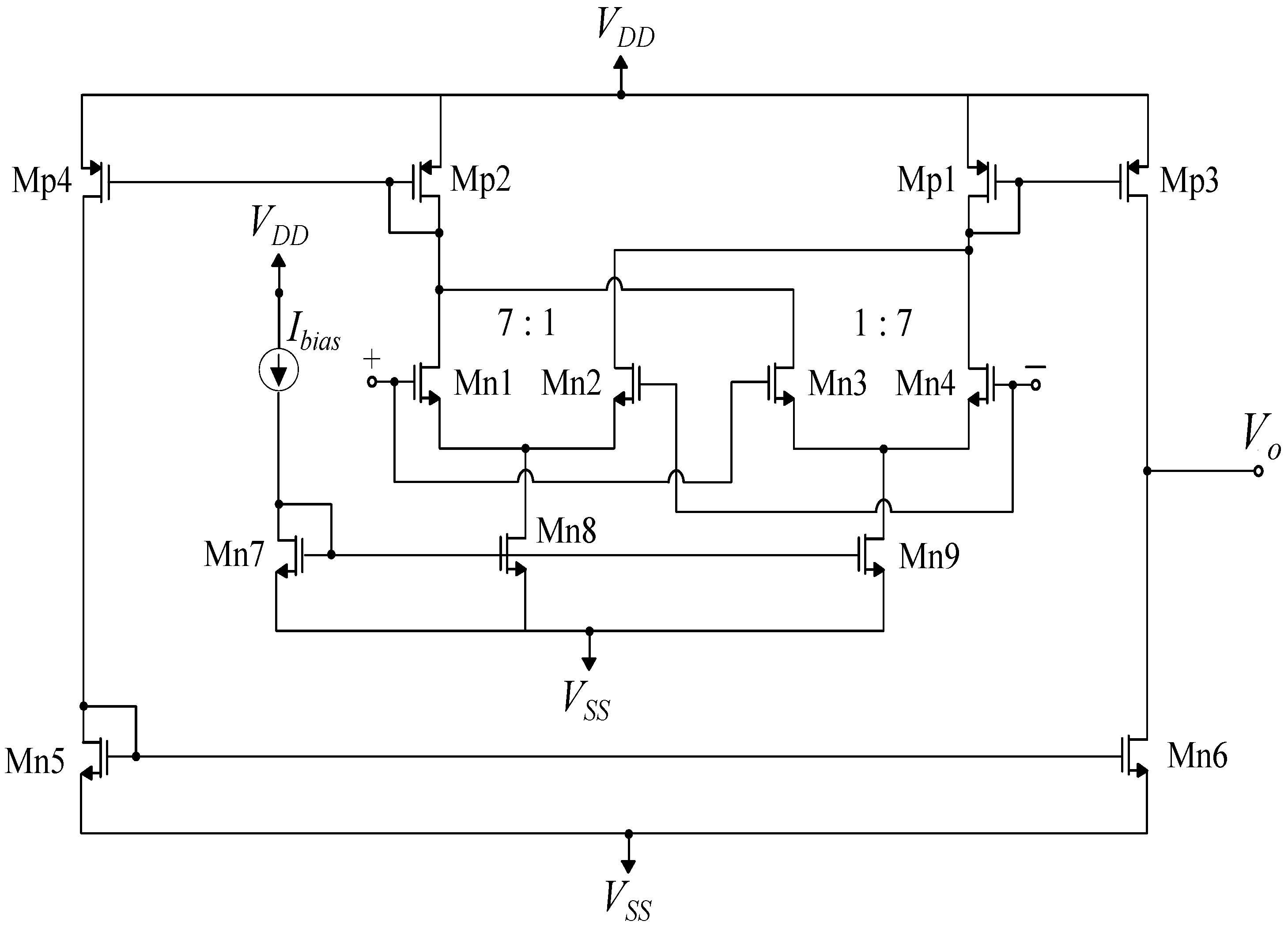
4.3. MIN/MAX Circuit
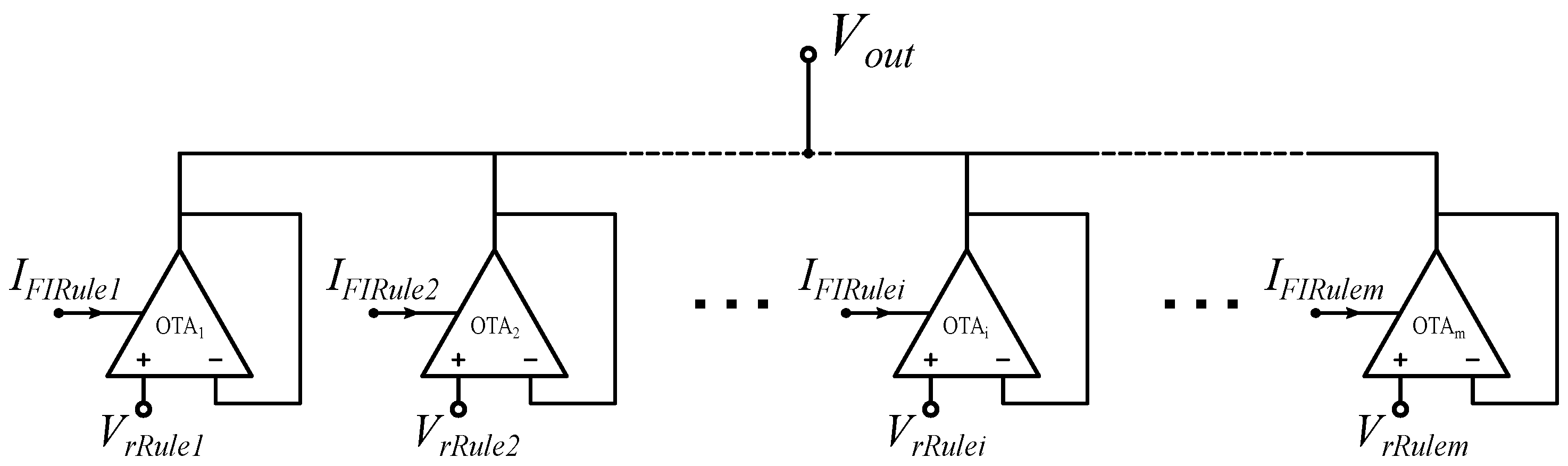
4.4. COG Circuit
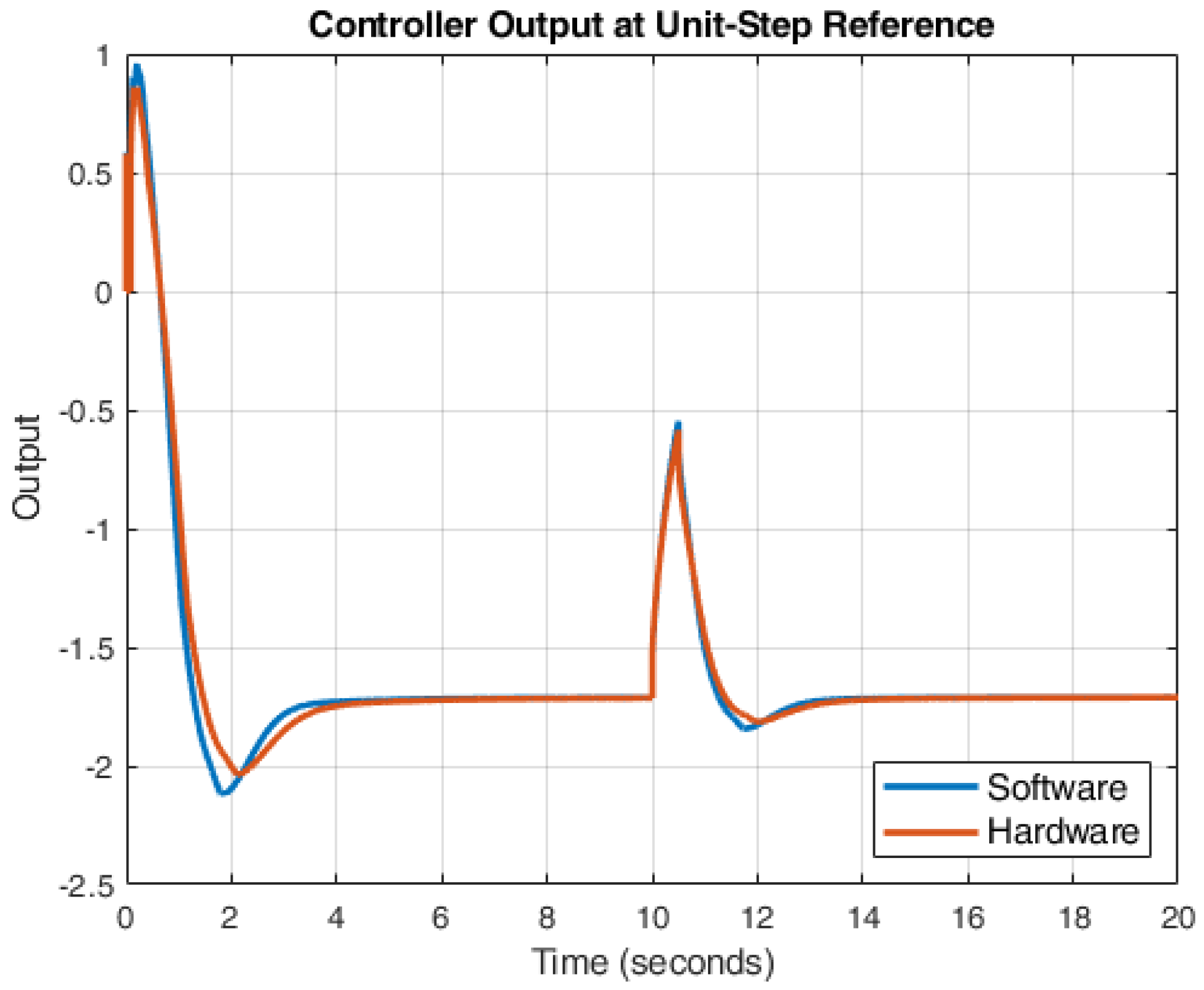
5. Application Example and Simulation Results
6. Conclusions
Author Contributions
Funding
Institutional Review Board Statement
Informed Consent Statement
Data Availability Statement
Conflicts of Interest
References
- Jang, H.; Topal, E. A review of soft computing technology applications in several mining problems. Appl. Soft Comput. 2014, 22, 638–651. [Google Scholar] [CrossRef]
- Zadeh, L.A. Soft computing and fuzzy logic. IEEE Softw. 1994, 11, 48–56. [Google Scholar] [CrossRef]
- Jang, J.; Sun, C.; Mizutani, E. Neuro-Fuzzy and Soft Computing: A Computational Approach to Learning and Machine Intelligence; MATLAB Curriculum Series; Prentice Hall: Upper Saddle River, NJ, USA, 1997. [Google Scholar]
- Zadeh, L.A. Fuzzy sets. Inf. Control 1965, 8, 338–353. [Google Scholar] [CrossRef]
- Seger, C.A.; Miller, E.K. Category learning in the brain. Annu. Rev. Neurosci. 2010, 33, 203–219. [Google Scholar] [CrossRef] [PubMed]
- Smithson, M.; Verkuilen, J. Fuzzy Set Theory: Applications in the Social Sciences; Number 147; Sage: Newcastle upon Tyne, UK, 2006. [Google Scholar]
- Pedrycz, W.; Gomide, F. An Introduction to Fuzzy Sets: Analysis and Design; MIT Press: Cambridge, MA, USA, 1998. [Google Scholar]
- Klir, G.; Yuan, B. Fuzzy Sets and Fuzzy Logic; Prentice Hall: Upper Saddle River, NJ, USA, 1995; Volume 4. [Google Scholar]
- Zadeh, L.A. A computational approach to fuzzy quantifiers in natural languages. In Computational Linguistics; Elsevier: Amsterdam, The Netherlands, 1983; pp. 149–184. [Google Scholar]
- Shihabudheen, K.; Pillai, G.N. Recent advances in neuro-fuzzy system: A survey. Knowl.-Based Syst. 2018, 152, 136–162. [Google Scholar]
- Carvajal, J.; Chen, G.; Ogmen, H. Fuzzy PID controller: Design, performance evaluation, and stability analysis. Inf. Sci. 2000, 123, 249–270. [Google Scholar] [CrossRef]
- Nguyen, H.T.; Prasad, N.R.; Walker, C.L.; Walker, E.A. A First Course in Fuzzy and Neural Control; CRC Press: Boca Raton, FL, USA, 2002. [Google Scholar]
- Jerry, M.M. Uncertain Rule-Based Fuzzy Systems: Introduction and New Directions; Springer: Berlin, Germany, 2019. [Google Scholar]
- Jantzen, J. Foundations of Fuzzy Control: A Practical Approach; John Wiley & Sons: Hoboken, NJ, USA, 2013. [Google Scholar]
- Al-Odienat, A.I.; Al-Lawama, A.A. The advantages of PID fuzzy controllers over the conventional types. Am. J. Appl. Sci. 2008, 5, 653–658. [Google Scholar] [CrossRef]
- Haensch, W.; Gokmen, T.; Puri, R. The next generation of deep learning hardware: Analog computing. Proc. IEEE 2018, 107, 108–122. [Google Scholar] [CrossRef]
- Bonissone, P.P.; Badami, V.; Chiang, K.H.; Khedkar, P.S.; Marcelle, K.W.; Schutten, M.J. Industrial applications of fuzzy logic at General Electric. Proc. IEEE 1995, 83, 450–465. [Google Scholar] [CrossRef]
- Sun, H.; Zhao, H.; Huang, K.; Qiu, M.; Zhen, S.; Chen, Y.H. A fuzzy approach for optimal robust control design of an automotive electronic throttle system. IEEE Trans. Fuzzy Syst. 2017, 26, 694–704. [Google Scholar] [CrossRef]
- Li, C.; Hu, R. Fuzzy-PID control for the regulation of blood glucose in diabetes. In Proceedings of the 2009 WRI Global Congress on Intelligent Systems, Xiamen, China, 19–21 May 2009; Volume 2, pp. 170–174. [Google Scholar]
- Kapoulea, S.; Yesil, A.; Psychalinos, C.; Minaei, S.; Elwakil, A.S.; Bertsias, P. Fractional-order and power-law shelving filters: Analysis and design examples. IEEE Access 2021, 9, 145977–145987. [Google Scholar] [CrossRef]
- Sacu, I.E.; Alci, M. Low-power OTA-C based tuneable fractional order filters. Electron. Components Mater. 2018, 48, 135–144. [Google Scholar]
- Valencia-Ponce, M.A.; González-Zapata, A.M.; de la Fraga, L.G.; Sanchez-Lopez, C.; Tlelo-Cuautle, E. Integrated Circuit Design of Fractional-Order Chaotic Systems Optimized by Metaheuristics. Electronics 2023, 12, 413. [Google Scholar] [CrossRef]
- Bertsias, P.; Safari, L.; Minaei, S.; Elwakil, A.; Psychalinos, C. Fractional-order differentiators and integrators with reduced circuit complexity. In Proceedings of the 2018 IEEE International Symposium on Circuits and Systems (ISCAS), Florence, Italy, 27–30 May 2018; pp. 1–4. [Google Scholar]
- Tsirimokou, G.; Psychalinos, C.; Elwakil, A.S.; Salama, K.N. Electronically tunable fully integrated fractional-order resonator. IEEE Trans. Circuits Syst. II Express Briefs 2017, 65, 166–170. [Google Scholar] [CrossRef]
- Sharma, R.; Rana, K.; Kumar, V. Performance analysis of fractional order fuzzy PID controllers applied to a robotic manipulator. Expert Syst. Appl. 2014, 41, 4274–4289. [Google Scholar] [CrossRef]
- Mohan, V.; Panjwani, B.; Chhabra, H.; Rani, A.; Singh, V. Self-regulatory fractional fuzzy control for dynamic systems: An analytical approach. Int. J. Fuzzy Syst. 2023, 25, 794–815. [Google Scholar] [CrossRef]
- Matusu, R. Application of fractional order calculus to control theory. Int. J. Math. Model. Methods Appl. Sci. 2011, 5, 1162–1169. [Google Scholar]
- Delavari, H.; Ghaderi, R.; Ranjbar, A.; Momani, S. Fuzzy fractional order sliding mode controller for nonlinear systems. Commun. Nonlinear Sci. Numer. Simul. 2010, 15, 963–978. [Google Scholar] [CrossRef]
- Yen, J. Fuzzy Logic: Intelligence, Control, and Information; Pearson Education: Noida, India, 1999. [Google Scholar]
- Yang, Q.; Yao, D.; Garnett, J.; Muller, K. Using a trust inference model for flexible and controlled information sharing during crises. J. Contingencies Crisis Manag. 2010, 18, 231–241. [Google Scholar] [CrossRef]
- Al-Turki, Y.A.; Attia, A.F.; Soliman, H.F. Optimization of fuzzy logic controller for supervisory power system stabilizers. Acta Polytech. 2012, 52, 7–16. [Google Scholar] [CrossRef]
- Arya, Y. A new optimized fuzzy FOPI-FOPD controller for automatic generation control of electric power systems. J. Frankl. Inst. 2019, 356, 5611–5629. [Google Scholar] [CrossRef]
- Arya, Y. Automatic generation control of two-area electrical power systems via optimal fuzzy classical controller. J. Frankl. Inst. 2018, 355, 2662–2688. [Google Scholar] [CrossRef]
- Liu, J.; Yang, O.W. Using fuzzy logic control to provide intelligent traffic management service for high-speed networks. IEEE Trans. Netw. Serv. Manag. 2013, 10, 148–161. [Google Scholar]
- Islam, M.S.; Bhuyan, M.; Azim, M.A.; Teng, L.; Othman, M. Hardware implementation of traffic controller using fuzzy expert system. In Proceedings of the 2006 International Symposium on Evolving Fuzzy Systems, Ambelside, UK, 7–9 September 2006; pp. 325–330. [Google Scholar]
- Madrigal Arteaga, V.M.; Pérez Cruz, J.R.; Hurtado-Beltrán, A.; Trumpold, J. Efficient Intersection Management Based on an Adaptive Fuzzy-Logic Traffic Signal. Appl. Sci. 2022, 12, 6024. [Google Scholar] [CrossRef]
- Sánchez-Solano, S.; Cabrera, A.J.; Baturone, I.; Moreno-Velo, F.J.; Brox, M. FPGA implementation of embedded fuzzy controllers for robotic applications. IEEE Trans. Ind. Electron. 2007, 54, 1937–1945. [Google Scholar] [CrossRef]
- Silva, S.N.; Lopes, F.F.; Valderrama, C.; Fernandes, M.A. Proposal of Takagi–Sugeno fuzzy-PI controller hardware. Sensors 2020, 20, 1996. [Google Scholar] [CrossRef]
- Varshavsky, V.; Marakhovsky, V.; Levin, I.; Saito, H. Hardware Implementation of Fuzzy Controllers. In Fuzzy Controller, Theory and Applications; In-Tech: Rijeka, Croatia, 2011; pp. 34–44. [Google Scholar]
- Uzunsoy, E. A brief review on fuzzy logic used in vehicle dynamics control. J. Innov. Sci. Eng. (JISE) 2018, 2, 1–7. [Google Scholar]
- Wang, Z.; Choi, S.B. A fuzzy sliding mode control of anti-lock system featured by magnetorheological brakes: Performance evaluation via the hardware-in-the-loop simulation. J. Intell. Mater. Syst. Struct. 2021, 32, 1580–1590. [Google Scholar] [CrossRef]
- Rubaai, A.; Ofoli, A.R.; Burge, L.; Garuba, M. Hardware implementation of an adaptive network-based fuzzy controller for DC-DC converters. IEEE Trans. Ind. Appl. 2005, 41, 1557–1565. [Google Scholar] [CrossRef]
- Bosque, G.; del Campo, I.; Echanobe, J. Fuzzy systems, neural networks and neuro-fuzzy systems: A vision on their hardware implementation and platforms over two decades. Eng. Appl. Artif. Intell. 2014, 32, 283–331. [Google Scholar] [CrossRef]
- Kuo, Y.H.; Kao, C.I.; Chen, J.J. A fuzzy neural network model and its hardware implementation. IEEE Trans. Fuzzy Syst. 1993, 1, 171–183. [Google Scholar] [CrossRef]
- Lotfy, A.; Kaveh, M.; Mosavi, M.; Rahmati, A. An enhanced fuzzy controller based on improved genetic algorithm for speed control of DC motors. Analog. Integr. Circuits Signal Process. 2020, 105, 141–155. [Google Scholar] [CrossRef]
- Herrera, F.; Lozano, M.; Verdegay, J.L. Tuning fuzzy logic controllers by genetic algorithms. Int. J. Approx. Reason. 1995, 12, 299–315. [Google Scholar] [CrossRef]
- Khan, S.; Abdulazeez, S.F.; Adetunji, L.W.; Alam, A.Z.; Salami, M.J.E.; Hameed, S.A.; Abdalla, A.H.; Islam, M.R. Design and implementation of an optimal fuzzy logic controller using genetic algorithm. J. Comput. Sci. 2008, 4, 799. [Google Scholar] [CrossRef]
- Caponetto, R.; Dongola, G.; Maione, G.; Pisano, A. Integrated technology fractional order proportional-integral-derivative design. J. Vib. Control. 2014, 20, 1066–1075. [Google Scholar] [CrossRef]
- Tepljakov, A.; Petlenkov, E.; Belikov, J. Efficient analog implementations of fractional-order controllers. In Proceedings of the 14th International Carpathian Control Conference (ICCC), Rytro, Poland, 26–29 May 2013; pp. 377–382. [Google Scholar]
- Psychalinos, C. Development of fractional-order analog integrated controllers—Application examples. Appl. Control 2019, 6, 357. [Google Scholar]
- Muñiz-Montero, C.; García-Jiménez, L.V.; Sánchez-Gaspariano, L.A.; Sánchez-López, C.; González-Díaz, V.R.; Tlelo-Cuautle, E. New alternatives for analog implementation of fractional-order integrators, differentiators and PID controllers based on integer-order integrators. Nonlinear Dyn. 2017, 90, 241–256. [Google Scholar] [CrossRef]
- Podlubny, I.; Petráš, I.; Vinagre, B.M.; O’Leary, P.; Dorčák, L. Analogue realizations of fractional-order controllers. Nonlinear Dyn. 2002, 29, 281–296. [Google Scholar] [CrossRef]
- Bohannan, G.W. Analog fractional order controller in temperature and motor control applications. J. Vib. Control. 2008, 14, 1487–1498. [Google Scholar] [CrossRef]
- Petráš, I. Fractional-order feedback control of a DC motor. J. Electr. Eng. 2009, 60, 117–128. [Google Scholar]
- Mokarram, M.; Khoei, A.; Hadidi, K. CMOS fuzzy logic controller supporting fractional polynomial membership functions. Fuzzy Sets Syst. 2015, 263, 112–126. [Google Scholar] [CrossRef]
- Johnson, M.A.; Moradi, M.H. PID Control; Springer: Berlin, Germany, 2005. [Google Scholar]
- Mousa, M.; Ebrahim, M.A.; Moustafa Hassan, M. Optimal fractional order proportional—integral—differential controller for inverted pendulum with reduced order linear quadratic regulator. In Fractional Order Control and Synchronization of Chaotic Systems; Springer: Berlin, Germany, 2017; pp. 225–252. [Google Scholar]
- Jamil, A.A.; Tu, W.F.; Ali, S.W.; Terriche, Y.; Guerrero, J.M. Fractional-order PID controllers for temperature control: A review. Energies 2022, 15, 3800. [Google Scholar] [CrossRef]
- Shah, P.; Agashe, S. Review of fractional PID controller. Mechatronics 2016, 38, 29–41. [Google Scholar] [CrossRef]
- Bingi, K.; Ibrahim, R.; Karsiti, M.N.; Hassan, S.M.; Harindran, V.R. Fractional-Order Systems and PID Controllers; Springer: Berlin, Germany, 2020; Volume 264. [Google Scholar]
- Sivanandam, S.; Sumathi, S.; Deepa, S. Introduction to Fuzzy Logic Using MATLAB; Springer: Berlin, Germany, 2007. [Google Scholar]
- Mamdani, E.H.; Assilian, S. An experiment in linguistic synthesis with a fuzzy logic controller. Int. J.-Man-Mach. Stud. 1975, 7, 1–13. [Google Scholar] [CrossRef]
- Pan, I.; Das, S.; Gupta, A. Tuning of an optimal fuzzy PID controller with stochastic algorithms for networked control systems with random time delay. ISA Trans. 2011, 50, 28–36. [Google Scholar] [CrossRef]
- Barakat, M. Optimal design of fuzzy-PID controller for automatic generation control of multi-source interconnected power system. Neural Comput. Appl. 2022, 34, 18859–18880. [Google Scholar] [CrossRef]
- Das, S.; Pan, I.; Das, S.; Gupta, A. A novel fractional order fuzzy PID controller and its optimal time domain tuning based on integral performance indices. Eng. Appl. Artif. Intell. 2012, 25, 430–442. [Google Scholar] [CrossRef]
- Buscarino, A.; Caponetto, R.; Graziani, S.; Murgano, E. Realization of fractional order circuits by a Constant Phase Element. Eur. J. Control 2020, 54, 64–72. [Google Scholar] [CrossRef]
- Abdelliche, F.; Charef, A.; Talbi, M.; Benmalek, M. A fractional wavelet for QRS detection. In Proceedings of the 2006 2nd International Conference on Information & Communication Technologies, Damascus, Syria, 24–28 April 2006; Volume 1, pp. 1186–1189. [Google Scholar]
- Benmalek, M.; Charef, A. Digital fractional order operators for R-wave detection in electrocardiogram signal. IET Signal Process. 2009, 3, 381–391. [Google Scholar] [CrossRef]
- Li, B.; Wu, J. Beta-expansion and continued fraction expansion. J. Math. Anal. Appl. 2008, 339, 1322–1331. [Google Scholar] [CrossRef]
- Chen, Y.; Vinagre, B.M.; Podlubny, I. Continued fraction expansion approaches to discretizing fractional order derivatives—An expository review. Nonlinear Dyn. 2004, 38, 155–170. [Google Scholar] [CrossRef]
- Colín-Cervantes, J.D.; Sánchez-López, C.; Ochoa-Montiel, R.; Torres-Muñoz, D.; Hernández-Mejía, C.M.; Sánchez-Gaspariano, L.A.; González-Hernández, H.G. Rational approximations of arbitrary order: A survey. Fractal Fract. 2021, 5, 267. [Google Scholar] [CrossRef]
- Tavazoei, M.S.; Haeri, M. Rational approximations in the simulation and implementation of fractional-order dynamics: A descriptor system approach. Automatica 2010, 46, 94–100. [Google Scholar] [CrossRef]
- Tsirimokou, G. A systematic procedure for deriving RC networks of fractional-order elements emulators using MATLAB. AEU Int. J. Electron. Commun. 2017, 78, 7–14. [Google Scholar] [CrossRef]
- Acay, B.; Inc, M. Electrical circuits RC, LC, and RLC under generalized type non-local singular fractional operator. Fractal Fract. 2021, 5, 9. [Google Scholar] [CrossRef]
- Lin, D.; Liao, X.; Dong, L.; Yang, R.; Samson, S.Y.; Iu, H.H.C.; Fernando, T.; Li, Z. Experimental study of fractional-order RC circuit model using the Caputo and Caputo-Fabrizio derivatives. IEEE Trans. Circuits Syst. I Regul. Pap. 2021, 68, 1034–1044. [Google Scholar] [CrossRef]
- Sen, F.; Kircay, A.; Cobb, B.S.; Karci, H. Current-mode fractional-order shelving filters using MCFOA for acoustic applications. AEU Int. J. Electron. Commun. 2023, 163, 154608. [Google Scholar] [CrossRef]
- Kartci, A.; Herencsar, N.; Machado, J.T.; Brancik, L. History and progress of fractional-order element passive emulators: A review. Radioengineering 2020, 29, 296–304. [Google Scholar] [CrossRef]
- Alimisis, V.; Dimas, C.; Pappas, G.; Sotiriadis, P.P. Analog realization of fractional-order skin-electrode model for tetrapolar bio-impedance measurements. Technologies 2020, 8, 61. [Google Scholar] [CrossRef]
- Alimisis, V.; Mouzakis, V.; Gennis, G.; Tsouvalas, E.; Sotiriadis, P.P. An Analog Nearest Class with Multiple Centroids Classifier Implementation, for Depth of Anesthesia Monitoring. In Proceedings of the 2022 International Conference on Smart Systems and Power Management (IC2SPM), Beirut, Lebanon, 10–12 November 2022; pp. 176–181. [Google Scholar]
- Alimisis, V.; Eleftheriou, N.P.; Kamperi, A.; Gennis, G.; Dimas, C.; Sotiriadis, P.P. General Methodology for the Design of Bell-Shaped Analog-Hardware Classifiers. Electronics 2023, 12, 4211. [Google Scholar] [CrossRef]
- Dualibe, C.; Verleysen, M.; Jespers, P. Design of Analog Fuzzy Logic Controllers in CMOS Technologies: Implementation, Test and Application; Springer Science & Business Media: Berlin, Germany, 2007. [Google Scholar]
- Sánchez-Gaspariano, L.A.; Díaz-Sánchez, A. CMOS Analog MAX/MIN operators: A qualitative comparsion. In Proceedings of the XV Congreso Interuniversitario de Electrónica, Computación y Eléctrica, Puebla, Mexico, 7–9 March 2005; pp. 7–9. [Google Scholar]
- Georgakilas, E.; Alimisis, V.; Gennis, G.; Aletraris, C.; Dimas, C.; Sotiriadis, P.P. An ultra-low power fully-programmable analog general purpose type-2 fuzzy inference system. AEU Int. J. Electron. Commun. 2023, 170, 154824. [Google Scholar] [CrossRef]
- Alikhani, A.; Ahmadi, A. A novel current-mode min–max circuit. Analog. Integr. Circuits Signal Process. 2012, 72, 343–350. [Google Scholar] [CrossRef]
- Baturone, I.; Sánchez-Solano, S.; Barriga, A.; Huertas, J. Implementation of inference/defuzzification methods via continuous-time analog circuits. In Proceedings of the IFSA World Congress, Sao Paulo, Brasil, 22–28 July 1995; pp. 623–626. [Google Scholar]
- Daneshvar, M.; Aminifar, S.; Yosefi, G. Design and Analysis of Current-Mode CMOS Analog Defuzzification Circuits for Fuzzy Controllers. J. Basic. Appl. Sci. Res. 2011, 1, 2488–2494. [Google Scholar]
- Mead, C.; Ismail, M. Analog VLSI Implementation of Neural Systems; Springer Science & Business Media: Berlin, Germany, 1989; Volume 80. [Google Scholar]
- Columbu, A.; Frassu, S.; Viglialoro, G. Properties of given and detected unbounded solutions to a class of chemotaxis models. arXiv 2023, arXiv:2303.15039. [Google Scholar] [CrossRef]
- Kumar, A.; Kumar, V. A novel interval type-2 fractional order fuzzy PID controller: Design, performance evaluation, and its optimal time domain tuning. ISA Trans. 2017, 68, 251–275. [Google Scholar] [CrossRef]
- Fuzzy Logic Toolbox. Available online: https://www.mathworks.com/products/fuzzy-logic.html (accessed on 10 December 2023).
- FOMCON Toolbox. Available online: https://www.mathworks.com/matlabcentral/fileexchange/66323-fomcon-toolbox-for-matlab (accessed on 10 December 2023).
- Cunillera, A.; Bešinović, N.; Lentink, R.M.; van Oort, N.; Goverde, R.M. A Literature Review on Train Motion Model Calibration. IEEE Trans. Intell. Transp. Syst. 2023, 24, 3660–3677. [Google Scholar] [CrossRef]


| Resistors | R () | Capacitors | C () |
|---|---|---|---|
| - | - | ||
| 20 | |||
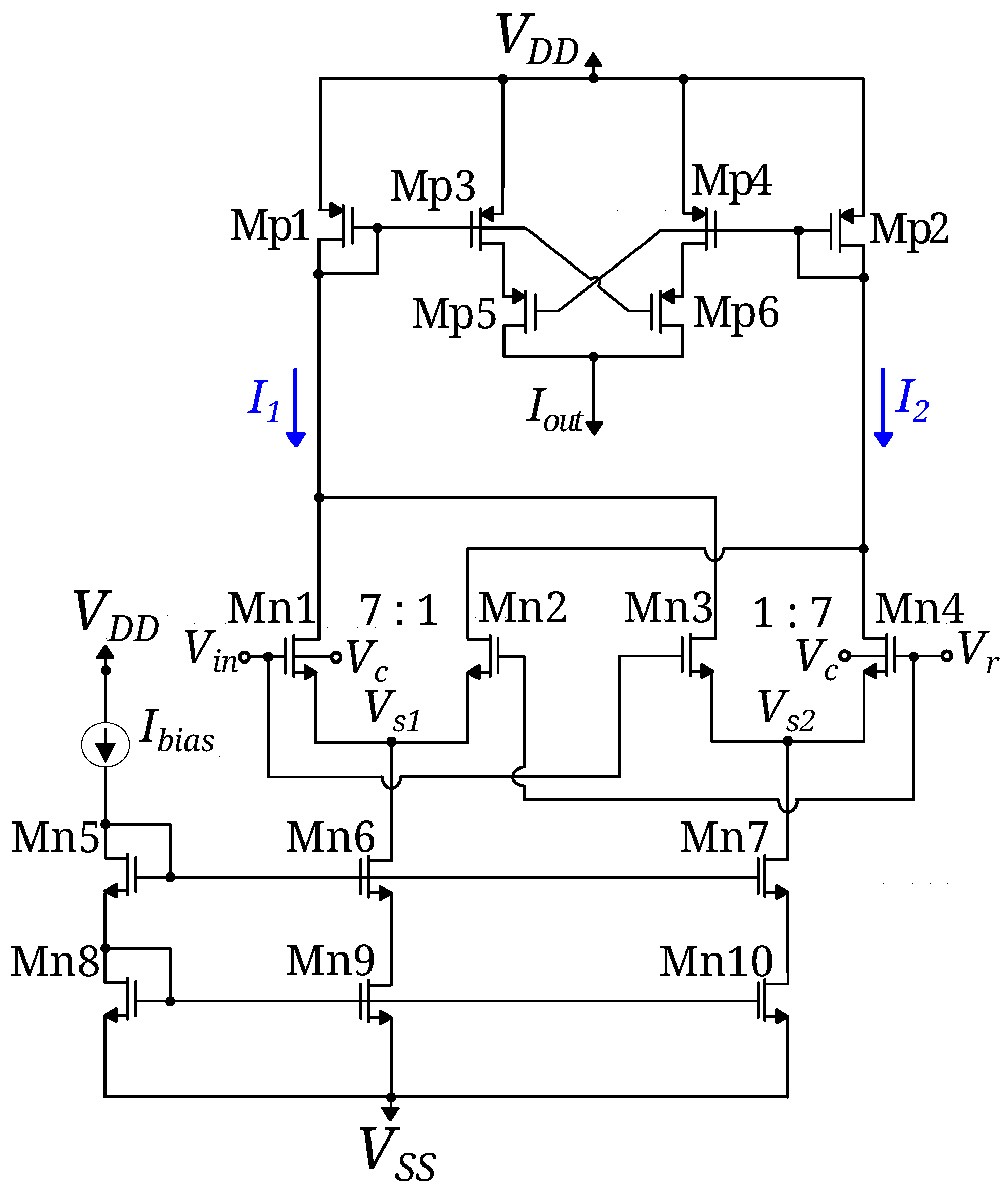
| NMOS Differential Block | W/L | Current Correlator | W/L |
|---|---|---|---|
| , | , | ||
| , | , | ||
| – | , | ||
| , | - | - |
| Differential Pair | W/L | Current Mirrors | W/L |
|---|---|---|---|
| , | , | ||
| , | , | ||
| , | |||
| , | - | - |
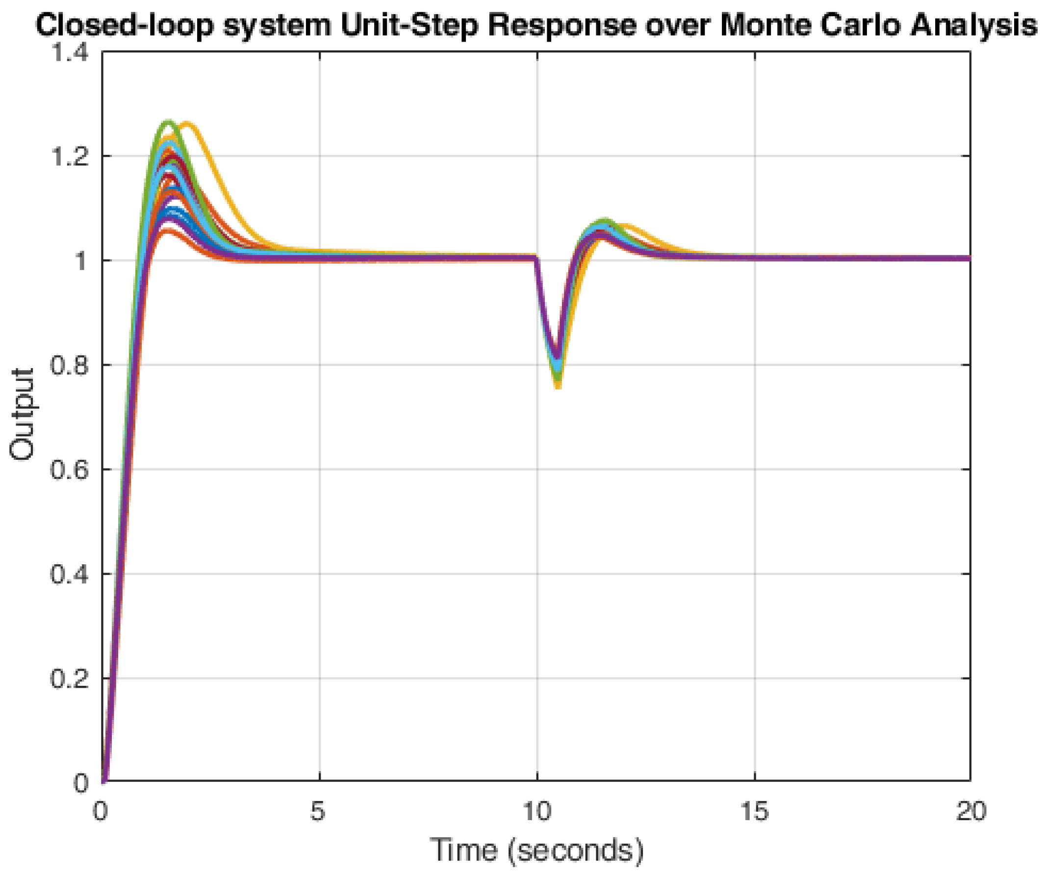
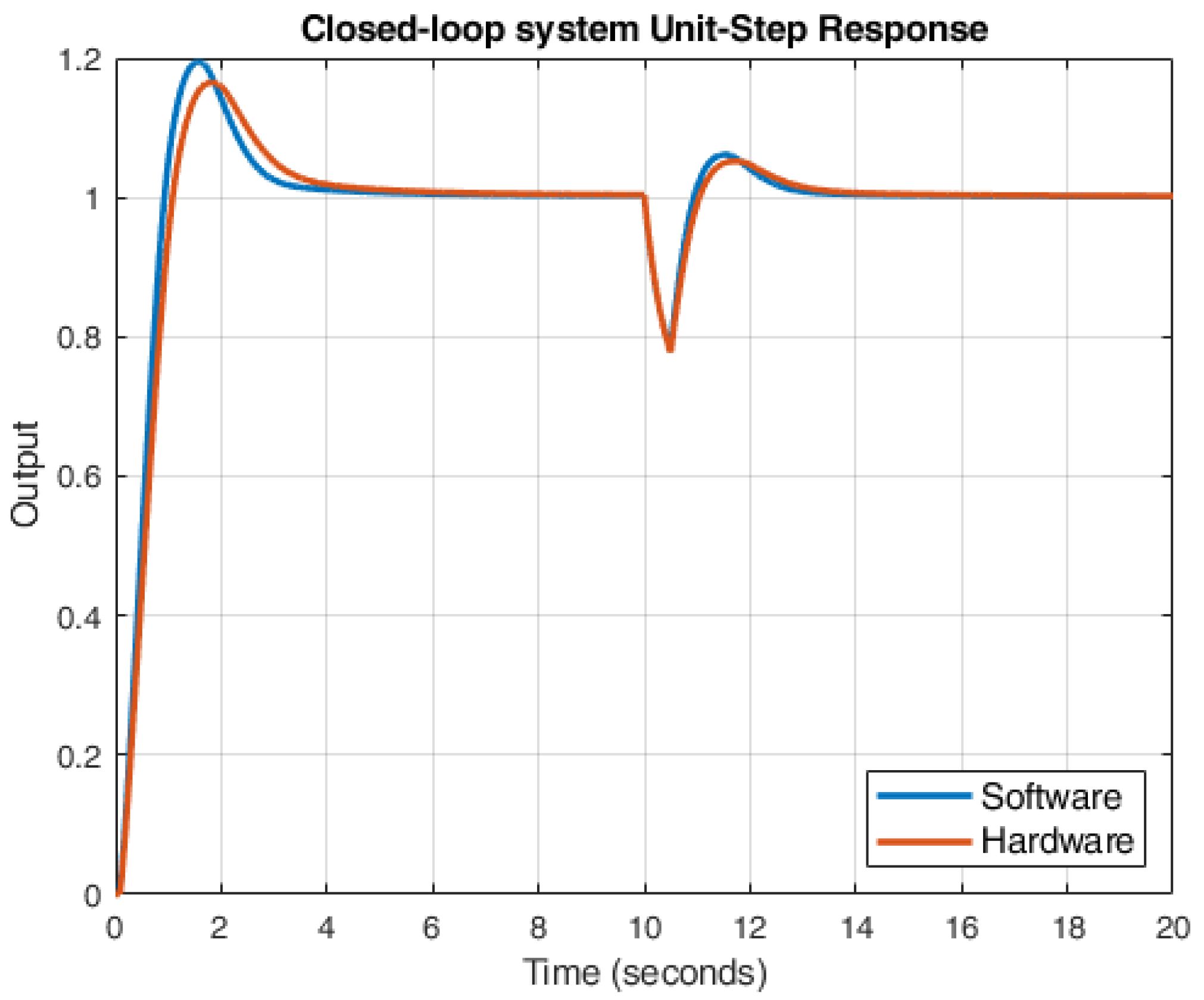
| KPI | Software | Hardware |
|---|---|---|
| Rise time (10–90%) | 0.54 s | 0.67 s |
| Overshot | 19.78% | 17.45% |
| Settling time | 3.97 s | 4.12 s |
| Steady-state error | 3.22% | 3.74% |
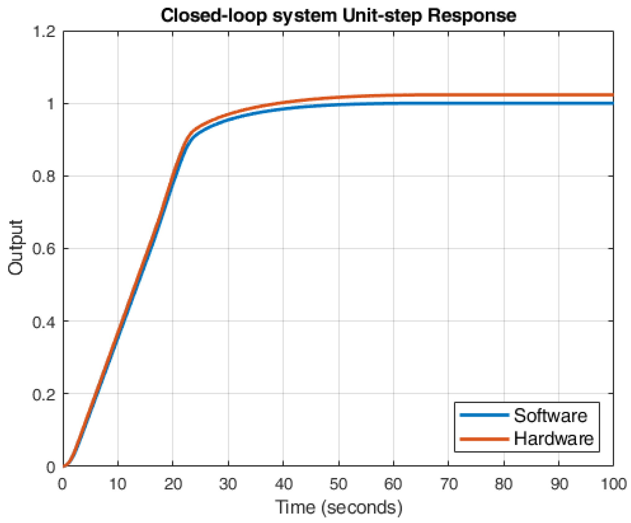
| KPI | Software | Hardware |
|---|---|---|
| Rise time (10–90%) | 19.62 s | 20.07 s |
| Overshot | 0% | 0% |
| Settling time | 48.71 s | 52.15 s |
| Steady-state error | 0.11% | 2.32% |
Disclaimer/Publisher’s Note: The statements, opinions and data contained in all publications are solely those of the individual author(s) and contributor(s) and not of MDPI and/or the editor(s). MDPI and/or the editor(s) disclaim responsibility for any injury to people or property resulting from any ideas, methods, instructions or products referred to in the content. |
© 2024 by the authors. Licensee MDPI, Basel, Switzerland. This article is an open access article distributed under the terms and conditions of the Creative Commons Attribution (CC BY) license (https://creativecommons.org/licenses/by/4.0/).
Share and Cite
Alimisis, V.; Eleftheriou, N.P.; Georgakilas, E.; Dimas, C.; Uzunoglu, N.; Sotiriadis, P.P. A Low Power Analog Integrated Fractional Order Type-2 Fuzzy PID Controller. Fractal Fract. 2024, 8, 234. https://doi.org/10.3390/fractalfract8040234
Alimisis V, Eleftheriou NP, Georgakilas E, Dimas C, Uzunoglu N, Sotiriadis PP. A Low Power Analog Integrated Fractional Order Type-2 Fuzzy PID Controller. Fractal and Fractional. 2024; 8(4):234. https://doi.org/10.3390/fractalfract8040234
Chicago/Turabian StyleAlimisis, Vassilis, Nikolaos P. Eleftheriou, Evangelos Georgakilas, Christos Dimas, Nikolaos Uzunoglu, and Paul P. Sotiriadis. 2024. "A Low Power Analog Integrated Fractional Order Type-2 Fuzzy PID Controller" Fractal and Fractional 8, no. 4: 234. https://doi.org/10.3390/fractalfract8040234
APA StyleAlimisis, V., Eleftheriou, N. P., Georgakilas, E., Dimas, C., Uzunoglu, N., & Sotiriadis, P. P. (2024). A Low Power Analog Integrated Fractional Order Type-2 Fuzzy PID Controller. Fractal and Fractional, 8(4), 234. https://doi.org/10.3390/fractalfract8040234