Research on Pattern Dynamics Behavior of a Fractional Vegetation-Water Model in Arid Flat Environment

Abstract

In order to stop and reverse land degradation and curb the loss of biodiversity, the United Nations 2030 Agenda for Sustainable Development proposes to combat desertification. In this paper, a fractional vegetation–water model in an arid flat environment is studied. The pattern behavior of the fractional model is much more complex than that of the integer order. We study the stability and Turing instability of the system, as well as the Hopf bifurcation of fractional order $\alpha$, and obtain the Turing region in the parameter space. According to the amplitude equation, different types of stationary mode discoveries can be obtained, including point patterns and strip patterns. Finally, the results of the numerical simulation and theoretical analysis are consistent. We find some novel fractal patterns of the fractional vegetation–water model in an arid flat environment. When the diffusion coefficient, d, changes and other parameters remain unchanged, the pattern structure changes from stripes to spots. When the fractional order parameter, $\beta$, changes, and other parameters remain unchanged, the pattern structure becomes more stable and is not easy to destroy. The research results can provide new ideas for the prevention and control of desertification vegetation patterns.

1. Introduction

In recent decades, desertification in arid and semi-arid regions has become more and more serious, and the United Nations has made combating desertification one of its global goals of sustainable development [1]. Semi-arid ecosystems are usually located at the edge of deserts. One side is the desert, and the other side is the vegetation, such as grass and shrubs [2]. It is estimated that semi-arid ecosystems cover about $30\%$ of the Earth’s surface [3], so it is critical to protect the sustainable development of vegetation systems.

Different vegetation growth conditions will lead to different spatial distributions of vegetation. The uneven distribution of vegetation across a space is known as a vegetation pattern [4]. It is a prominent feature of many semi-arid regions [5], and its appearance is often an early warning indicator of the transformation of ecosystems to desertification [6,7]. In 1999, Klausmeier [8] first proposed a vegetation water model to study desertification as follows:

$$\begin{array}{c}\hfill \left\{\begin{array}{c}{u}_t=\stackrel{uptakebyplants}{\overbrace{-Ru{v}^2}}+\stackrel{rainfall}{\overbrace{A}}-\stackrel{evaporation}{\overbrace{Lu}}+\stackrel{flowdownhill}{\overbrace{M{u}_x,}}\hfill \\ v_t=\underset{plantgrowth}{\underbrace{RJu{v}^2}}-\underset{plantloss}{\underbrace{Nv}}+\underset{dispersal}{\underbrace{D{\Delta }_{x,y}v}},\hfill \end{array}\right.\end{array}$$

(1)

with two variables, surface water $u\left(x,t\right)$ and vegetation $v\left(x,t\right)$. Here, A denotes precipitation under natural conditions, $Lu$ denotes water evaporation, $Ru{v}^2$ denotes the amount of water absorbed by plants, $M{u}_x$ denotes the downhill flow of water, $RJu{v}^2$ denotes the growth of plants themselves, $Nv$ denotes the loss of plants, D denotes the rate of vegetation diffusion, ${\Delta }_{x,y}$ denotes the Laplace operator. In ecology, all parameters are nonnegative constants.

Klausmeier’s model focuses on the flow pattern of water down the slope and cannot predict the flow pattern on the flat ground $\left(M=0\right)$. However, vegetation patterns were also observed in semi-arid ecosystems without slopes. In order to simulate the diffusion of water on a flat surface, researchers [9,10] used $d{\Delta }_{x,y}u$ instead of the advection term of $M{u}_x$ to extend model (1) and considered the following model:

$$\begin{array}{c}\hfill \left\{\begin{array}{c}{u}_t=-Ru{v}^2+A-Lu+d_1{\Delta }_{x,y}u,\hfill \\ v_t=RJu{v}^2-Nv+d_2{\Delta }_{x,y}v.\hfill \end{array}\right.\end{array}$$

(2)

For model (2), Wang et al. [9] proved that there is a non-uniform vegetation state when the rainfall is low. Sun et al. [11] discussed the wavelength variation with biological parameters and found different types of stationary modes. Guo et al. [12] described the evolution of vegetation patterns under different parameters. It is worth noting that model (2) is the same as the autocatalytic chemical reaction model proposed by Gray and Scott [13,14], so model (2) is also called the diffusion Klausmeier–Gray–Scott model [7]. In [15,16], Han et al. solved several types of reaction–diffusion equations using spatially discretized Fourier transform. In [17], Liu et al.introduced a time two-grid finite element method and derived the stability and error estimates of the fully discretized equation. In [18], Zhai et al. proposed a method to simulate the fractional Gray–Scott model by combining the semi-implicit spectral deferred correction method with the operator splitting scheme, and so on [19,20,21].

The succession of arid ecosystems can span a long duration, sometimes extending over hundreds of years. Influenced by climate, soil, and other regional factors, the succession process of each region may also vary. Due to the locality of integer order derivatives, there are some limitations in describing succession. Fractional derivatives are more suitable for description than integer derivatives due to their memorability and nonlocality. In order to understand the relationship between vegetation and water in arid ecosystems, we consider the following fractional-order models:

$$\begin{array}{c}\hfill \left\{\begin{array}{c}{\mathbf{D}}_t^{\alpha }u=-Ru{v}^2+A-Lu+D_1{\Delta }_{x,y}^{\beta }u,\hfill \\ {\mathbf{D}}_t^{\alpha }v=RJu{v}^2-Nv+D_2{\Delta }_{x,y}^{\beta }v.\hfill \end{array}\right.\end{array}$$

(3)

Here, ${\mathbf{D}}_t^{\alpha }$ represents Caputo fractional differentiation, and is defined as follows:

$$\begin{array}{c}\hfill \begin{array}{c}{\mathbf{D}}_t^{\alpha }u\left(t\right)=\frac{1}{\Gamma \left(1-\alpha \right)}{\int }_0^t\left(t-\tau \right)u^{\prime }\left(\tau \right)\mathrm{d}\tau \hfill \end{array},t>0,\end{array}$$

with $0<\alpha <1$.

The rest of this article is organized as follows. In Section 2, we establish a model and explore the positivity and uniqueness of solutions for models without diffusion terms. In Section 3, we discuss the stability of the model and Hopf bifurcation. In Section 4, the Turing instability of the model is discussed. In Section 5, weak nonlinear analysis is used to derive the amplitude equation. In Section 6, we conduct numerical simulations. We present our conclusion in Section 7.

2. Model and Preliminaries

Positive and Uniqueness

In this section, we prove the positive uniqueness and nonnegativity of solutions for fractional order models without diffusion terms.

The non-diffusion version of model (3) is as follows:

$$\begin{array}{c}\hfill \left\{\begin{array}{c}{\mathbf{D}}_t^{\alpha }u=-Ru{v}^2+A-Lu,\hfill \\ {\mathbf{D}}_t^{\alpha }v=RJu{v}^2-Nv.\hfill \end{array}\right.\end{array}$$

(4)

Lemma 1

([22]). Suppose $0<\alpha \le 1$, $f\left(t\right)\in C\left[a,b\right]$ and ${\mathbf{D}}_t^{\alpha }f\left(t\right)$ is continuous in $\left[a,b\right]$. For $t\in \left(a,b\right)$,

1. If ${\mathbf{D}}_t^{\alpha }f\left(t\right)\ge 0$, $f\left(t\right)$ is a non-decreasing function in $\left[a,b\right]$.

2. If ${\mathbf{D}}_t^{\alpha }f\left(t\right)\le 0$, $f\left(t\right)$ is a non-increasing function in $\left[a,b\right]$.

Let ${\mathbb{R}}^{+}$ represent the set of all nonnegative real numbers and ${\mathbb{C}}_{+}=\left\{\left(u,v\right)\in \mathbb{C}:u,v\in {\mathbb{R}}^{+}\right\}$.

Theorem 1.

All solutions of model (4), starting from ${\mathbb{C}}_{+}$, are nonnegative.

Proof .

Assume that there is a constant, $t_1$, satisfying $0\le t\le t_1$ and

$$\begin{array}{c}\hfill \left\{\begin{array}{c}v\left(t\right)>0,0\le t<t_1,\hfill \\ v\left(t_1\right)=0,\hfill \\ v\left(t_1^{+}\right)<0.\hfill \end{array}\right.\end{array}$$

(5)

From model (4), we can see the following:

$$\begin{array}{c}\hfill {\mathbf{D}}_t^{\alpha }v\left(t\right){\mid }_{v\left(t_1\right)=0}=0.\end{array}$$

(6)

Thus, from Lemma (1), $v\left(t_1^{+}\right)=0$ is not consistent with the assumption $v\left(t_1^{+}\right)<0$. Hence, $v\left(t\right)\ge 0$ for all $t\ge 0$. The same method can be applied to demonstrate that all solutions of model (4) are nonnegative. □

Theorem 2.

Fractional model (4) has a unique solution under any nonnegative initial conditions.

Proof .

According to the method proposed in [23,24,25], we define the following operator:

$$\begin{array}{c}\hfill \left\{\begin{array}{c}{f}_1\left(t,u\right)=-Ru{v}^2+A-Lu,\hfill \\ f_2\left(t,u\right)=RJu{v}^2-Nvv.\hfill \end{array}\right.\end{array}$$

(7)

Let

$$\begin{array}{c}\hfill N_1=\underset{C_{[a,b_1]}}{sup}\left|\right|f_1\left(t,u\right)\left|\right|,N_2=\underset{C_{[a,b_2]}}{sup}\left|\right|f_2\left(t,v\right)\left|\right|,\end{array}$$

(8)

with

$$\begin{array}{cc}\hfill C_{[a,b_1]}& =\left[t-a,t+a\right]\times \left[u-b_1,u+b_1\right]=A_1\times B_1,\hfill \\ \hfill C_{[a,b_2]}& =\left[t-a,t+a\right]\times \left[v-b_2,v+b_2\right]=A_2\times B_2.\hfill \end{array}$$

Using the Banach fixed point theorem, we can obtain the following uniform norm:

$$\begin{array}{c}\hfill \left|\right|f\left(t\right){\left|\right|}_{\infty }=sup\left|f\left(t\right)\right|,t\in \left[t-a,t+a\right].\end{array}$$

(9)

Picard’s operator is as follows:

$$\begin{array}{c}\hfill O:C\left(A_1,B_1,B_2\right)\to C\left(A_1,B_1,B_2\right).\end{array}$$

(10)

It is defined as follows:

$$\begin{array}{c}\hfill OX\left(t\right)=X_0\left(t\right)+\frac{1}{\Gamma \left(\alpha \right)}{\int }_0^t{\left(t-\tau \right)}^{\alpha -1}F\left(\tau ,X\left(\tau \right)\right)d\tau ,\end{array}$$

(11)

where $X\left(t\right)={\left[u\left(t\right),v\left(t\right)\right]}^T,X_0\left(t\right)={\left[u_0\left(t\right),v_0\left(t\right)\right]}^T,F\left(t,X\left(t\right)\right)={\left[f_1\left(t,u\right),f_2\left(t,v\right)\right]}^T$.

We assume that the solution of the model is bounded in a time period:

$$\begin{array}{c}\hfill \left|\right|X\left(t\right){\left|\right|}_{\infty }\le max\left\{b_1,b_2\right\}.\end{array}$$

(12)

We can obtain the following:

$$\begin{array}{c}\hfill \begin{array}{cc}\left|\right|OX\left(t\right)-X_0\left(t\right)\left|\right|\hfill & =\left|\right|\frac{1}{\Gamma \left(\alpha \right)}{\int }_0^t{\left(t-\tau \right)}^{\alpha -1}F\left(\tau ,X\left(\tau \right)\right)d\tau \left|\right|\hfill \\ & \le \frac{1}{\Gamma \left(\alpha \right)}{\int }_0^t{\left(t-\tau \right)}^{\alpha -1}\left|\right|F\left(\tau ,X\left(\tau \right)\right)\left|\right|d\tau \le \frac{N{a}^{\alpha }}{\Gamma \left(\alpha \right)}\le aN\le b,\hfill \end{array}\end{array}$$

(13)

with $N=max\left\{N_1,N_2\right\},b=max\left\{b_1,b_2\right\},a<\frac{b}{N}$.

$$\begin{array}{c}\hfill \begin{array}{cc}\left|\right|O{X}_1\left(t\right)-O{X}_2\left(t\right)\left|\right|\hfill & =\left|\right|\frac{1}{\Gamma \left(\alpha \right)}{\int }_0^t{\left(t-\tau \right)}^{\alpha -1}\left\{F\left(\tau ,X_1\left(\tau \right)\right)-F\left(\tau ,X_2\left(\tau \right)\right)\right\}d\tau \left|\right|\hfill \\ & \le \frac{1}{\Gamma \left(\alpha \right)}{\int }_0^t{\left(t-\tau \right)}^{\alpha -1}\left|\right|F\left(\tau ,X_1\left(\tau \right)\right)-F\left(\tau ,X_2\left(\tau \right)\right)\left|\right|d\tau \hfill \\ & \le \frac{\beta }{\Gamma \left(\alpha \right)}{\int }_0^t{\left(t-\tau \right)}^{\alpha -1}\left|\right|X_1\left(\tau \right)-X_2\left(\tau \right)\left|\right|d\tau \hfill \\ & \le \frac{\beta a^{\alpha }}{\Gamma \left(\alpha \right)}\left|\right|X_1\left(\tau \right)-X_2\left(\tau \right)\left|\right|\le a\beta \left|\right|X_1\left(\tau \right)-X_2\left(\tau \right)\left|\right|.\hfill \end{array}\end{array}$$

(14)

Since F is a contraction and $\beta <1$, we obtain $a\beta <1$; that is, the defined operator O is also a contraction. Therefore, the uniqueness proof of the system solution is completed. □

3. Stability and Hopf Bifurcation Analysis

In this part, we first discuss the number of equilibrium points of the model. Then, by analyzing the stability of the equilibrium point and the Hopf bifurcation, the conditions under which different states of the system appear are given. At the same time, numerical simulations are also used to prove the rationality of the theory.

3.1. Equilibrium Point

We obtain the equilibrium point by solving the following system of equations:

$$\begin{array}{c}\hfill \left\{\begin{array}{c}f\left(u,v\right)=-Ru{v}^2+A-Lu,\hfill \\ g\left(u,v\right)=RJu{v}^2-Nv.\hfill \end{array}\right.\end{array}$$

(15)

Denote by $f\left(u,v\right)=0$ and $g\left(u,v\right)=0$. The system (15) has a catalyst-free equilibrium point, $E_1=\left(\frac{A}{L},0\right)$, and a coexistence equilibrium point, $E_{*}=\left(u_{*},v_{*}\right)$. Then, we have the following:

$$\begin{array}{c}\hfill u_{*}=\frac{AJ-\sqrt{\frac{R{A}^2{J}^2-4L{N}^2}{R}}}{2JL},v_{*}=\frac{AJ+\sqrt{\frac{R{A}^2{J}^2-4L{N}^2}{R}}}{2N}.\end{array}$$

(16)

3.2. Stability Analysis

Before determining the stability of the equilibrium point, we first give the stability criterion of the fractional differential system.

Theorem 3

([26,27]). Consider a fractional differential system, as follows:

$$\begin{array}{c}\hfill {\mathbf{D}}_t^{\alpha }x\left(t\right)=f\left(t,x\left(t\right)\right).\end{array}$$

(17)

Let $x_{*}$ be an equilibrium point, and let ${\lambda }_i,\left(i=1,2,\cdots ,n\right)$ be the eigenvalues of the Jacobian matrix, $J=\frac{\partial f}{\partial x_{*}}$.

(1) The equilibrium point $x_{*}$ is asymptotically stable if and only if

$$\begin{array}{c}\hfill \left|arg\left({\lambda }_i\right)\right|>\alpha \frac{\pi }{2},i=1,2,\cdots ,n.\end{array}$$

(18)

(2) The equilibrium point $x_{*}$ is stable if and only if

$$\begin{array}{c}\hfill \left|arg\left({\lambda }_i\right)\right|\ge \alpha \frac{\pi }{2},i=1,2,\cdots ,n.\end{array}$$

(19)

(3) The equilibrium point $x_{*}$ is unstable if and only if

$$\begin{array}{c}\hfill \exists :\left|arg\left({\lambda }_i\right)\right|<\alpha \frac{\pi }{2},i=1,2,\cdots ,n.\end{array}$$

(20)

Definition 1

([28]). The roots of the equation $f\left(t,x\left(t\right)\right)=0$ are called the equilibria of the fractional differential system:

$$\begin{array}{c}\hfill {\mathbf{D}}_t^{\alpha }x\left(t\right)=f\left(t,x\left(t\right)\right),\end{array}$$

where $x\left(t\right)={\left(x_1\left(t\right),x_2\left(t\right),\cdots ,x_n\left(t\right)\right)}^T\in {\mathbb{R}}^n,f\left(t,x\left(t\right)\right)\in R^n$, and ${\mathbf{D}}_t^{\alpha }x\left(t\right)={\left({\mathbf{D}}_t^{{\alpha }_1}{x}_1\left(t\right),{\mathbf{D}}_t^{{\alpha }_2}{x}_2\left(t\right),\cdots ,{\mathbf{D}}_t^{{\alpha }_n}{x}_n\left(t\right)\right)}^T,{\alpha }_i\in {\mathbb{R}}^{+},i=1,2,\cdots ,n$.

We can obtain the Jacobi matrix for system (15) at the equilibrium point, $E_1$, as follows:

$$\begin{array}{c}\hfill J=\left(\begin{array}{cc}{a}_{11}& a_{12}\\ a_{21}& a_{22}\end{array}\right)=\left(\begin{array}{cc}-L& 0\\ 0& -N\end{array}\right),\end{array}$$

(21)

Two eigenvalues are ${\lambda }_1<0,{\lambda }_2<0$; therefore, $\left|arg\left({\lambda }_{1,2}\right)\right|=\pi >\alpha \frac{\pi }{2}$ implies $E_1$ is asymptotically stable;

The Jacobian matrix of system (15) at the equilibrium point, $E_{*}$, is as follows:

$$\begin{array}{c}\hfill J=\left(\begin{array}{cc}{a}_{11}& a_{12}\\ a_{21}& a_{22}\end{array}\right)=\left(\begin{array}{cc}-\frac{AJR\left(AJ-\sqrt{\frac{R{A}^2{J}^2-4L{N}^2}{R}}\right)}{2N^2}& -\frac{2N}{J}\\ \frac{JR{\left(AJ-\sqrt{\frac{R{A}^2{J}^2-4L{N}^2}{R}}\right)}^2}{4N^2}& N\end{array}\right).\end{array}$$

(22)

As such, the characteristic equation at equilibrium point $E_{*}$ is as follows:

$$\begin{array}{c}\hfill {\lambda }^2-t{r}_0\lambda +de{t}_0=0,\end{array}$$

(23)

where

$$\begin{array}{c}\hfill t{r}_0=\frac{-R{A}^2{J}^2+2N^3+AJR{\left(AJ-B\right)}^2}{2N^2},de{t}_0=\frac{-R\left(AJ-B\right)B}{2N},\end{array}$$

(24)

with $B=\sqrt{\frac{R{A}^2{J}^2-4L{N}^2}{R}}$.

The roots of the characteristic equations are as follows:

$$\begin{array}{c}\hfill {\lambda }_{1,2}=\frac{t{r}_0\pm \sqrt{\Delta }}{2},\Delta =t{r}_0^2-4de{t}_0.\end{array}$$

(25)

The eigenvalues are real when $\Delta \ge 0$. For $t{r}_0=0$, ${\lambda }_{1,2}=\pm i\sqrt{{det}_0}$ is obtained; therefore $\left|arg\left({\lambda }_{1,2}\right)\right|=\frac{\pi }{2}>\alpha \frac{\pi }{2}$ implies $E_{*}$ is asymptotically stable. The eigenvalues are negative real when $t{r}_0<0$ and $de{t}_0>0$, so $\left|arg\left({\lambda }_{1,2}\right)\right|=\pi >\alpha \frac{\pi }{2}$ implies $E_{*}$ is asymptotically stable. For $t{r}_0>0$ and $de{t}_0>0$, both the eigenvalues are positive real; hence, $\left|arg\left({\lambda }_{1,2}\right)\right|=0<\alpha \frac{\pi }{2}$ implies $E_{*}$ is unstable. When $de{t}_0<0$, the two eigenvalues are real numbers with opposite signs, so $\left|arg\left({\lambda }_1\right)\right|=0<\alpha \frac{\pi }{2}$ implies that $E_{*}$ is unstable. The two eigenvalues are complex conjugates when $\Delta <0$. In this case, the definition is as follows:

$$\begin{array}{c}\hfill \frac{\alpha \pi }{2}=\left|{tan}^{-1}\left(\frac{\sqrt{4{det}_0-t{r}_0^2}}{t{r}_0}\right)\right|.\end{array}$$

(26)

Therefore, $E_{*}$ is stable if $\alpha \frac{\pi }{2}<\left|{tan}^{-1}\left(\frac{\sqrt{4{det}_0-t{r}_0^2}}{t{r}_0}\right)\right|$ and is unstable for $\alpha \frac{\pi }{2}>\left|{tan}^{-1}\left(\frac{\sqrt{4{det}_0-t{r}_0^2}}{t{r}_0}\right)\right|$.

Through Theorem 3, we draw the following conclusions:

Theorem 4.

The system is asymptotically stable at the equilibrium point $E_1=\left(\frac{A}{L},0\right)$.

Theorem 5

([29]). The stability of equilibrium point $E_{*}$ is determined by $t{r}_0,de{t}_0$ and α.

If $\Delta \ge 0$, then we have the following:

(1) the equilibrium point, $E_{*}$, is asymptotically stable if and only if $t{r}_0\le 0$ and $de{t}_0>0$.

(2) the equilibrium point, $E_{*}$, is unstable if and only if $t{r}_0>0$ or $de{t}_0<0$.

If $\Delta <0$, then:

(3) the equilibrium point, $E_{*}$, is stable if and only if $\alpha \frac{\pi }{2}<\left|{tan}^{-1}\left(\frac{\sqrt{4{det}_0-t{r}_0^2}}{t{r}_0}\right)\right|$.

(4) the equilibrium point, $E_{*}$, is unstable if and only if $\alpha \frac{\pi }{2}>\left|{tan}^{-1}\left(\frac{\sqrt{4{det}_0-t{r}_0^2}}{t{r}_0}\right)\right|$.

3.3. Hopf Bifurcation Analysis

When $t{r}_0=0$ and $de{t}_0>0$, model (4) with $\alpha =1$ loses stability through Hopf bifurcation. Since the stability of model (4) is affected by the fractional derivative, the fractional derivative can be regarded as a parameter of the Hopf bifurcation. In the following, we establish the conditions for the Hopf bifurcation of model (4) around $E_{*}$ at parameter $\alpha ={\alpha }_h$ [30,31]:

(1) The Jacobian matrix at the equilibrium point, $E_{*}$, has a pair of complex conjugate eigenvalues ${\lambda }_{1,2}=a_i+i{b}_i$, which become purely imaginary when $\alpha ={\alpha }_h$.

(2) $m\left({\alpha }_h\right)=0$ where $m\left(\alpha \right)=\alpha \frac{\pi }{2}-{\displaystyle \underset{1\le i\le 2}{min}}\left|arg\left({\lambda }_i\right)\right|$.

(3) ${\left.\frac{\partial m\left(\alpha \right)}{\partial \alpha }\right|}_{\alpha ={\alpha }_h}\ne 0$.

Now, we prove that $E_{*}$ has a Hopf bifurcation when $\alpha$ goes through ${\alpha }_h$.

Theorem 6.

Suppose that the equilibrium point, $E_{*}$, is unstable when $\Delta <0$ and $t{r}_0>0$. The fractional parameter, α, passes through the critical value, ${\alpha }_h$, and model (4) undergoes the Hopf bifurcation near $E_{*}$, where

$$\begin{array}{c}\hfill {\alpha }_h=\frac{2}{\pi }{tan}^{-1}\left(\frac{\sqrt{4{det}_0-t{r}_0^2}}{t{r}_0}\right).\end{array}$$

(27)

Proof .

For $\Delta <0$ and $t{r}_0>0$, the eigenvalues are complex conjugates with positive real parts. Hence, we have the following:

$$\begin{array}{c}\hfill 0<arg\left({\lambda }_{12}\right)={tan}^{-1}\left(\frac{\sqrt{4{det}_0-t{r}_0^2}}{t{r}_0}\right)<\frac{\pi }{2},\end{array}$$

(28)

and $\alpha \frac{\pi }{2}>\left|{tan}^{-1}\left(\frac{\sqrt{4{det}_0-t{r}_0^2}}{t{r}_0}\right)\right|$ for some α. Let ${\alpha }_h\frac{\pi }{2}=\left|{tan}^{-1}\left(\frac{\sqrt{4{det}_0-t{r}_0^2}}{t{r}_0}\right)\right|$, obtain ${\alpha }_h=\frac{2}{\pi }{tan}^{-1}\left(\frac{\sqrt{4{det}_0-t{r}_0^2}}{t{r}_0}\right)$. Moreover, ${\left.\frac{\partial m\left(\alpha \right)}{\partial \alpha }\right|}_{\alpha ={\alpha }_h}=\frac{\pi }{2}\ne 0$. Therefore, all Hopf conditions are satisfied. □

Remark 1.

Now, we use fractional Adams–Bashforth-Moulton methods [32] for the numerical simulation to provide evidence that supports these viewpoints. We use the parameter values given in Table 1, and the selection of parameter values refers to the relevant published paper [12].

Table 1. The parameter values for the numerical study of model (4).

R	J	A	L	N
1	1	13.9	1	5.5

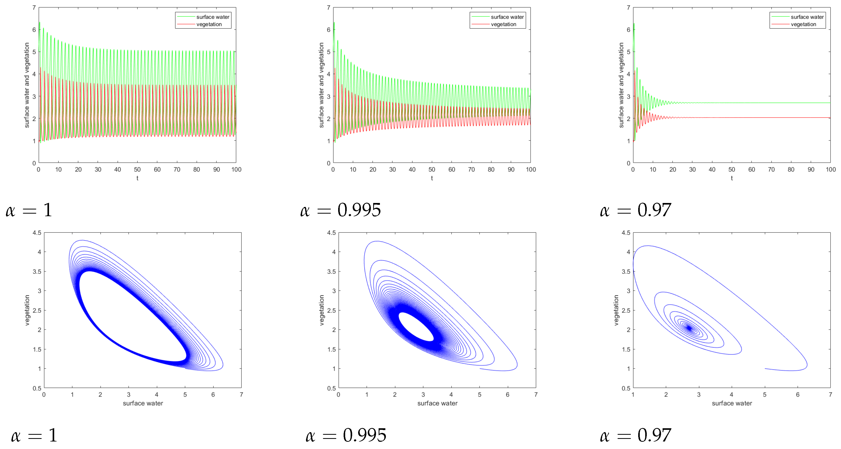
At the equilibrium point $E_{*}=\left(11.199,0.49109\right)$, the conditions $t{r}_0=4.2588,{det}_0=-4.1736$ and $\Delta =34.832$ are satisfied, which conforms to Theorem 5. Therefore, the equilibrium point is unstable, and there is a stable limit cycle around it. See Figure 1. The decrease in the fractional order parameter $\alpha$ value corresponds to the increase in the memory effect in the model. As it decreases, the equilibrium point, $E_{*}$, maintains an unstable spiral, and the circumference of the limit cycle also decreases. This situation continues until reaching the critical Hopf bifurcation value ${\alpha }_h=0.994$. For $\alpha <{\alpha }_h$, the equilibrium point, $E_{*}$, of the system becomes a stable spiral. Therefore, the memory effect drives the model to exhibit stable behavior. From an ecological point of view, it can be inferred that both surface water and vegetation use some of their past behavior in the ecosystem to establish sustainable development. For example, vegetation adapts to the environment by thickening roots.

Figure 1. Time series and phase diagrams of surface water and vegetation in model (4) under different fractional order parameters $\alpha$.

4. Turing Instability

In this section, we present the Turing instability condition for model (3).

We perturb the equilibrium point with $u=u_{*}+\tilde{u},v=v_{*}+\tilde{v}$, substitute it into model (3), expand it through the Taylor series, remove higher-order terms, and obtain the linear perturbation equation, as follows:

$$\begin{array}{c}\hfill \dot{U}=JU+D\Delta U,\end{array}$$

(29)

where

$$\begin{array}{c}\hfill U=\left(\begin{array}{c}\tilde{u}\\ \tilde{v}\end{array}\right),D=\left(\begin{array}{cc}{d}_1& \\ & d_2\end{array}\right).\end{array}$$

(30)

J is a Jacobian matrix at $E_{*}$. For convenience, we still denote $\tilde{u}$ and $\tilde{v}$ as u and v.

Expanding the perturbation variables in Fourier space and substituting $U=\left(\begin{array}{c}{c}_k^1\\ c_k^2\end{array}\right)e^{\lambda t+ikr}$ into the perturbation Equation (29) yields the characteristic equation, as follows:

$$\begin{array}{c}\hfill \lambda \left(\begin{array}{c}{c}_k^1\\ c_k^2\end{array}\right)=\left(\begin{array}{cc}{a}_{11}-k^2{d}_1& a_{12}\\ a_{21}& a_{22}-k^2{d}_2\end{array}\right)\left(\begin{array}{c}{c}_k^1\\ c_k^2\end{array}\right),\end{array}$$

(31)

where $\lambda$ is the growth rate, k is the wave number, r is the spatial vector, and $c_k^1,c_k^2$ are constants.

We solve characteristic Equation (31) and obtain the following dispersion relationship:

$$\begin{array}{c}\hfill {\lambda }^2-t{r}_k\lambda +de{t}_k=0,\end{array}$$

(32)

where

$$\begin{array}{c}\hfill \left\{\begin{array}{c}t{r}_k=a_{11}+a_{22}-k^2\left(d_1+d_2\right)=t{r}_0-k^2\left(d_1+d_2\right),\hfill \\ \underset{k}{det}=a_{11}{a}_{22}-a_{21}{a}_{12}-k^2\left(a_{11}{d}_2+a_{22}{d}_1\right)+k^4{d}_1{d}_2=\underset{0}{det}-k^2\left(a_{11}{d}_2+a_{22}{d}_1\right)+k^4{d}_1{d}_2.\hfill \end{array}\right.\end{array}$$

The solution of characteristic Equation (32) is in the following form:

$$\begin{array}{c}\hfill {\lambda }_k=\frac{t{r}_k\pm \sqrt{t{r}_k^2-4{det}_k}}{2}.\end{array}$$

(33)

In order to explore the existence conditions for Turing instability at $k\ne 0$, we should ensure that $t{r}_k<0$ and $de{t}_k<0$. In order to ensure the occurrence of $de{t}_k<0$, the condition of marginal stability $min\left(det\left(k_c^2\right)\right)=0$ should be satisfied. Here, $k_c^2=\frac{a_{11}{d}_2+a_{22}{d}_1}{2d_1{d}_2}$ is the minimum value of $de{t}_k$ with respect to $k_c^2$.

From $min\left(det\left(k_c^2\right)\right)=0$, we can obtain

$$\begin{array}{c}\hfill a_{22}^2{d}_1^2+2d_2\left(a_{11}{a}_{22}-2de{t}_0\right)d_1+a_{11}^2{d}_2^2=0.\end{array}$$

Since $E_{*}$ is a positive equilibrium point, ${det}_0>0,a_{11}{a}_{22}$ can be obtained, so we have the following:

$$\begin{array}{c}\hfill d_1^{+}=\frac{d_2\left(2{det}_0-a_{11}{a}_{22}\right)+2d_2\sqrt{{det}_0\left({det}_0-a_{11}{a}_{22}\right)}}{a_{22}^2}>0,\\ \hfill d_1^{-}=\frac{d_2\left(2{det}_0-a_{11}{a}_{22}\right)-2d_2\sqrt{{det}_0\left({det}_0-a_{11}{a}_{22}\right)}}{a_{22}^2}>0.\end{array}$$

Theorem 7.

Suppose that $0\le r\le 1$ and $d_1>0,d_2>0$ are valid.

(1) The equilibrium point, $E_{*}$, is asymptotically stable if and only if $d_{+}^{-}<d_1<d_1^{+}$.

(2) The equilibrium point, $E_{*}$, is unstable if and only if $d_1>d_{+}^{-}$ or $d_1<d_{+}^{-}$.

(3) Turing bifurcation occurs at $d_1=d_{+}^{-}$ or $d_1=d_{+}^{-}$, and the critical wave number is $k_c^2=\sqrt{\frac{{det}_0}{d_1^{+}{d}_2}}$ or $k_c^2=\sqrt{\frac{{det}_0}{d_1^{-}{d}_2}}$.

Proof .

The eigenvalues are negative real when $d_{+}^{-}<d_1<d_1^{+}$, so $\left|arg\left({\lambda }_k\right)\right|=\pi >\alpha \frac{\pi }{2}$ implies $E_{*}$ is asymptotically stable;

When $d_1>d_{+}^{-}$ or $d_1<d_{+}^{-}$, the two eigenvalues are real numbers with opposite signs, so $\left|arg\left({\lambda }_k\right)\right|=0<\alpha \frac{\pi }{2}$ implies $E_{*}$ is unstable;

From $min\left(det\left(k_c^2\right)\right)=0$, we have $k_c^2=\sqrt{\frac{{det}_0}{d_1^{+}{d}_2}}$ or $k_c^2=\sqrt{\frac{{det}_0}{d_1^{-}{d}_2}}$. □

Remark 2.

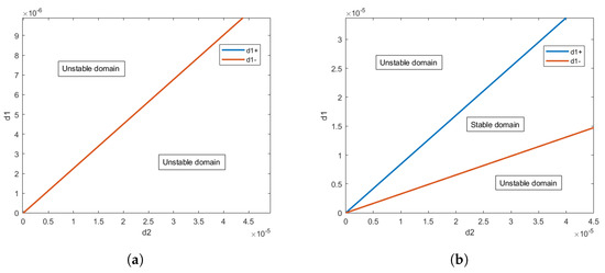
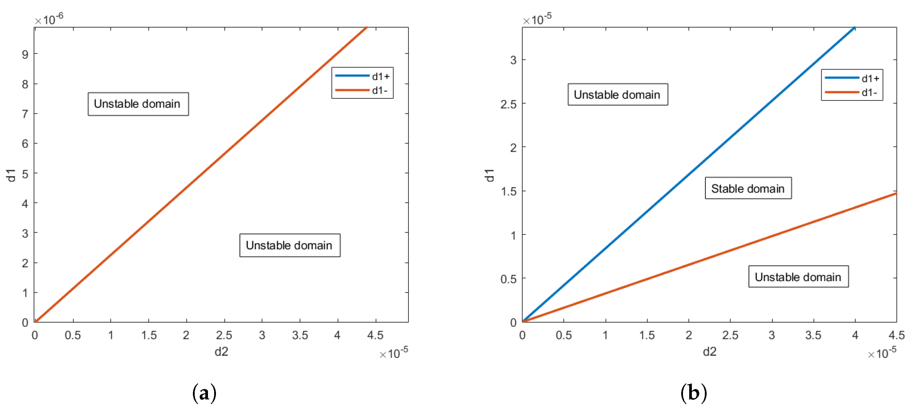
Take $R=1,J=1,A=0.014,L=0.014,N=0.062,d_2=0.00001$. We draw the stable region of equilibrium point E on the plane when $d_1>0,d_2>0$. According to Theorem 7, the stable region and the unstable region are distinguished in Figure 2.

Figure 2. Stability domains of equilibrium (a) $E_1$ and (b) $E_{*}$.

5. Weakly Nonlinear Analysis

In this section, we use weak nonlinear analysis to calculate the amplitude equation near the Turing instability threshold, $d_1=d_1^c$. We write model (3) in the following form:

$$\begin{array}{c}\hfill \frac{\partial U}{\partial t}=LU+N\left(U,U\right),\end{array}$$

(34)

where L is a linear operator and N is a nonlinear operator.

$$\begin{array}{c}\hfill L=\left(\begin{array}{cc}{a}_{11}+d_1\Delta & a_{12}\\ a_{21}& a_{22}+d_2\Delta \end{array}\right),\end{array}$$

(35)

and

$$\begin{array}{c}\hfill N=\left(\begin{array}{c}-2R{v}_{*}uv-R{u}_{*}{v}^2-Ru{v}^2\\ 2JR{v}_{*}uv+JR{u}_{*}{v}^2+JRu{v}^2\end{array}\right)+\mathcal{O}\left(4\right).\end{array}$$

(36)

We only consider the behavior of the control parameter near the bifurcation point, so the control parameter, $d_1$, can be expanded as follows:

$$\begin{array}{c}\hfill d_1-d_1^c=\epsilon d_{11}+{\epsilon }^2{d}_{12}+{\epsilon }^3{d}_{13}+\mathcal{O}\left(4\right),\end{array}$$

(37)

where $\epsilon$ is a small parameter. At the same time, the variable, U, and the nonlinear term, N, are expanded according to this small parameter:

$$\begin{array}{c}\hfill U=\left(\begin{array}{c}u\\ v\end{array}\right)=\epsilon \left(\begin{array}{c}{u}_1\\ v_1\end{array}\right)+{\epsilon }^2\left(\begin{array}{c}{u}_2\\ v_2\end{array}\right)+{\epsilon }^3\left(\begin{array}{c}{u}_3\\ v_3\end{array}\right)+\mathcal{O}\left(4\right),\end{array}$$

(38)

$$\begin{array}{c}\hfill N={\epsilon }^2{N}_2+{\epsilon }^3{N}_3+\mathcal{O}\left({\epsilon }^4\right),\end{array}$$

(39)

with

$$\begin{array}{c}\hfill N_2=\left(\begin{array}{c}-2R{v}_{*}{u}_1{v}_1-R{u}_{*}{v}_1^2\\ 2JR{v}_{*}{u}_1{v}_1+JR{u}_{*}{v}_1^2\end{array}\right),\end{array}$$

(40)

and

$$\begin{array}{c}\hfill N_3=\left(\begin{array}{c}-2R{v}_{*}\left(u_1{v}_2+u_2{v}_1\right)-2R{u}_{*}{v}_1{v}_2-R{u}_1{v}_1^2\\ 2JR{v}_{*}\left(u_1{v}_2+u_2{v}_1\right)+2JR{u}_{*}{v}_1{v}_2+JR{u}_1{v}_1^2\end{array}\right).\end{array}$$

(41)

The linear operator, L, can be decomposed into the following:

$$\begin{array}{c}\hfill L=L_c+\left(d_1-d_1^c\right)M,\end{array}$$

where

$$\begin{array}{c}\hfill L_c=\left(\begin{array}{cc}{a}_{11}+d_1^c\Delta & a_{12}\\ a_{21}& a_{22}+d_2\Delta \end{array}\right),M=\left(\begin{array}{cc}\Delta & 0\\ 0& 0\end{array}\right).\end{array}$$

(42)

We set $T_0=t,T_1=\epsilon t,T_2={\epsilon }^{2}t,T_3={\epsilon }^{3}t$; then, the partial derivative of time can be written as follows:

$$\begin{array}{c}\hfill \frac{\partial }{\partial t}=\epsilon \frac{\partial }{\partial T_1}+{\epsilon }^2\frac{\partial }{\partial T_2}+{\epsilon }^3\frac{\partial }{\partial T_3}+\mathcal{O}\left(4\right).\end{array}$$

(43)

We substitute Formulas (37)–(43) into Equation (34).

The left side of the equation is as follows:

$$\begin{array}{c}\epsilon \frac{\partial }{\partial t}\left(\begin{array}{c}{u}_1\hfill \\ v_1\hfill \end{array}\right)+{\epsilon }^2\frac{\partial }{\partial t}\left(\begin{array}{c}{u}_2\\ v_2\end{array}\right)+{\epsilon }^3\frac{\partial }{\partial t}\left(\begin{array}{c}{u}_3\\ v_3\end{array}\right)=\\ \begin{array}{c}\hfill \epsilon \left[\epsilon \frac{\partial }{\partial T_1}\left(\begin{array}{c}{u}_1\\ v_1\end{array}\right)+{\epsilon }^2\frac{\partial }{\partial T_2}\left(\begin{array}{c}{u}_1\\ v_1\end{array}\right)+{\epsilon }^3\frac{\partial }{\partial T_3}\left(\begin{array}{c}{u}_1\\ v_1\end{array}\right)\right]+{\epsilon }^2\left[\epsilon \frac{\partial }{\partial T_1}\left(\begin{array}{c}{u}_2\\ v_2\end{array}\right)+{\epsilon }^2\frac{\partial }{\partial T_2}\left(\begin{array}{c}{u}_2\\ v_2\end{array}\right)+{\epsilon }^3\frac{\partial }{\partial T_3}\left(\begin{array}{c}{u}_2\\ v_2\end{array}\right)\right]+...,\end{array}\end{array}$$

The right side of the equation is as follows:

$$\begin{array}{c}\hfill \left[L_c+\left(\epsilon d_{11}+{\epsilon }^2{d}_{12}+{\epsilon }^3{d}_{13}\right)M\right]\left[\epsilon \left(\begin{array}{c}{u}_1\\ v_1\end{array}\right)+{\epsilon }^2\left(\begin{array}{c}{u}_2\\ v_2\end{array}\right)+{\epsilon }^3\left(\begin{array}{c}{u}_3\\ v_3\end{array}\right)\right]+{\epsilon }^2{N}_2+{\epsilon }^3{N}_3.\end{array}$$

(44)

Comparing the order of $\epsilon$ on both sides of the equation, the following three cases are obtained:

$$\begin{array}{c}\hfill \epsilon :L_c\left(\begin{array}{c}{u}_1\\ v_1\end{array}\right)=0,\end{array}$$

(45)

$$\begin{array}{c}\hfill {\epsilon }^2:L_c\left(\begin{array}{c}{u}_2\\ v_2\end{array}\right)=\frac{\partial }{\partial T_1}\left(\begin{array}{c}{u}_1\\ v_1\end{array}\right)-d_{11}M\left(\begin{array}{c}{u}_1\\ v_1\end{array}\right)-N_2,\end{array}$$

(46)

$$\begin{array}{c}\hfill {\epsilon }^3:L_c\left(\begin{array}{c}{u}_3\\ v_3\end{array}\right)=\frac{\partial }{\partial T_1}\left(\begin{array}{c}{u}_2\\ v_2\end{array}\right)+\frac{\partial }{\partial T_2}\left(\begin{array}{c}{u}_1\\ v_1\end{array}\right)-d_{11}M\left(\begin{array}{c}{u}_2\\ v_2\end{array}\right)-d_{12}M\left(\begin{array}{c}{u}_1\\ v_1\end{array}\right)-N_3.\end{array}$$

(47)

They are discussed separately, as follows:

$\mathcal{O}\left(\epsilon \right)$:

$$\begin{array}{c}\hfill L_c\left(\begin{array}{c}{u}_1\\ v_1\end{array}\right)=0.\end{array}$$

(48)

That is, $\left(\begin{array}{c}{u}_1\\ v_1\end{array}\right)$ is a linear combination of eigenvectors corresponding to eigenvalues of 0. Therefore,

$$\begin{array}{c}\hfill \left(\begin{array}{cc}{a}_{11}+d_1^c{k}_c^2& a_{12}\\ a_{21}& a_{22}+d_2{k}_c^2\end{array}\right)\left(\begin{array}{c}{u}_1\\ v_1\end{array}\right)=0,\end{array}$$

(49)

The general solution of Equation (45) can be written as follows:

$$\begin{array}{c}\hfill \left(\begin{array}{c}{u}_1\\ v_1\end{array}\right)=\left(\begin{array}{c}\varphi \\ 1\end{array}\right)\left(\sum _{j=1}^3{A}_j{e}^{i{k}_{j}r}+\sum _{j=1}^3{\overline{A}}_j{e}^{-i{k}_{j}r}\right),\end{array}$$

(50)

where $\varphi =-\frac{a_{22}+d_2{k}_c^2}{a_{21}}$, $|k_j|=k_c$, $k_c^2=\sqrt{\frac{{det}_0}{d_1{d}_2}}$, $k_j$ denotes the amplitude of the mode $e^{-i{k}_{j}r}$.

$\mathcal{O}\left({\epsilon }^2\right)$

$$\begin{array}{c}\hfill \left(\begin{array}{c}{P}_u\\ P_v\end{array}\right)=\frac{\partial }{\partial T_1}\left(\begin{array}{c}{u}_1\\ v_1\end{array}\right)-d_{11}M\left(\begin{array}{c}{u}_1\\ v_1\end{array}\right)-N_2.\end{array}$$

(51)

According to the Fredholm solvability condition, the vector function on the right side of Equation (51) must be orthogonal to the zero eigenvalue of $L_c^{+}$ for this equation to have a nontrivial solution.

$$\begin{array}{c}\hfill L_c^{+}=\left(\begin{array}{cc}{a}_{11}+d_1^c\Delta & a_{21}\\ a_{12}& a_{22}+d_2\Delta \end{array}\right).\end{array}$$

The zero eigenvector of

$$\begin{array}{c}\hfill \left(\begin{array}{c}1\\ \phi \end{array}\right)e^{-i{k}_{j}r}+c.c.,j=1,2,3,\end{array}$$

with $\phi =-\frac{a_{12}}{a_{22}+d_2{k}_c^2}$. According to the orthogonal condition of Equation (46), we have

$$\begin{array}{c}\hfill \left(1,\phi \right)\left(\begin{array}{c}{P}_u^j\\ P_v^j\end{array}\right)=0,j=1,2,3,\end{array}$$

(52)

where $P_u^j$ and $P_v^j$ are the coefficients corresponding to $e^{i{k}_{j}r}$ in $P_u$ and $P_v$. The system of equations related to amplitude $A_j$, obtained from Equation (52), is as follows:

$$\begin{array}{c}\hfill \left\{\begin{array}{c}\left(\varphi +\phi \right)\frac{\partial A_1}{\partial T_1}=-d_{11}{k}_c^2\varphi A_1+2\left(h_1+\phi h_2\right){\overline{A}}_2{\overline{A}}_3,\\ \left(\varphi +\phi \right)\frac{\partial A_2}{\partial T_1}=-d_{11}{k}_c^2\varphi A_2+2\left(h_1+\phi h_2\right){\overline{A}}_1{\overline{A}}_3,\\ \left(\varphi +\phi \right)\frac{\partial A_3}{\partial T_1}=-d_{11}{k}_c^2\varphi A_3+2\left(h_1+\phi h_2\right){\overline{A}}_1{\overline{A}}_2,\end{array}\right.\end{array}$$

(53)

where $h_1=-2v_{*}\varphi -u_{*},h_2=2v_{*}\varphi +u_{*}$. We introduce a second-order disturbance term as follows:

$$\begin{array}{c}\hfill \left(\begin{array}{c}{u}_2\\ v_2\end{array}\right)=\left(\begin{array}{c}{U}_0\\ V_0\end{array}\right)+\sum _{j=1}^3\left(\begin{array}{c}{U}_j\\ V_j\end{array}\right)e^{i{k}_{j}r}+\sum _{j=1}^3\left(\begin{array}{c}{U}_{jj}\\ V_{jj}\end{array}\right)e^{2i{k}_{j}r}+\left(\begin{array}{c}{U}_{12}\\ V_{12}\end{array}\right)e^{i\left(k_1-k_2\right)r}+\\ \hfill \left(\begin{array}{c}{U}_{23}\\ V_{23}\end{array}\right)e^{i\left(k_2-k_3\right)r}+\left(\begin{array}{c}{U}_{31}\\ V_{31}\end{array}\right)e^{i\left(k_3-k_1\right)r}+c.c,\end{array}$$

(54)

We substitute Formulas (50) and (54) into Equation (46). We have the following:

$$\begin{array}{c}\hfill U_j=\varphi V_j,j=1,2,3,\left(\begin{array}{c}{U}_0\hfill \\ V_0\hfill \end{array}\right)=\left(\begin{array}{c}{u}_0^0\hfill \\ v_0^0\hfill \end{array}\right)\left(|A_1{|}^2+|A_2{|}^2+{\left|A_3\right|}^2\right),\\ \hfill \left(\begin{array}{c}{U}_{jj}\hfill \\ V_{jj}\hfill \end{array}\right)=\left(\begin{array}{c}{u}_1^1\hfill \\ v_1^1\hfill \end{array}\right)A_j^2,j=1,2,3,\left(\begin{array}{c}{U}_{ij}\hfill \\ V_{ij}\hfill \end{array}\right)=\left(\begin{array}{c}{u}_2^2\hfill \\ v_2^2\hfill \end{array}\right)A_i{\overline{A}}_j,i\ne j,i=j=1,2,3.\end{array}$$

with

$$\begin{array}{c}\left(\begin{array}{c}{u}_0^0\\ v_0^0\end{array}\right)=\left(\begin{array}{c}\frac{2\left(a_{12}{h}_2-a_{22}{h}_1\right)}{a_{11}{a}_{22}-a_{12}{a}_{21}}\\ \frac{2\left(a_{21}{h}_1-a_{11}{h}_2\right)}{a_{11}{a}_{22}-a_{12}{a}_{21}}\end{array}\right),\left(\begin{array}{c}{u}_1^1\\ v_1^1\end{array}\right)=\left(\begin{array}{c}\frac{a_{12}{h}_2-\left(a_{22}-4d_2{k}_c^2\right)h_1}{\left(a_{11}-4d_1^c{k}_c^2\right)\left(a_{22}-4d_2{k}_c^2\right)-a_{12}{a}_{21}}\\ \frac{a_{21}{h}_1-\left(a_{11}-4d_1{k}_c^2\right)h_2}{\left(a_{11}-4d_1^c{k}_c^2\right)\left(a_{22}-4d_2{k}_c^2\right)-a_{12}{a}_{21}}\end{array}\right),\\ \left(\begin{array}{c}{u}_2^2\\ v_2^2\end{array}\right)=\left(\begin{array}{c}\frac{2\left[a_{12}{h}_2-\left(a_{22}-3d_2{k}_c^2\right)h_1\right]}{\left(a_{11}-3d_1^c{k}_c^2\right)\left(a_{22}-3d_2{k}_c^2\right)-a_{12}{a}_{21}}\\ \frac{2\left[a_{21}{h}_1-\left(a_{11}-3d_1{k}_c^2\right)h_2\right]}{\left(a_{11}-3d_1^c{k}_c^2\right)\left(a_{22}-3d_2{k}_c^2\right)-a_{12}{a}_{21}}\end{array}\right).\end{array}$$

$\mathcal{O}\left({\epsilon }^3\right)$

$$\begin{array}{c}\hfill \left(\begin{array}{c}{P}_u\\ P_v\end{array}\right)=\frac{\partial }{\partial T_1}\left(\begin{array}{c}{u}_2\\ v_2\end{array}\right)+\frac{\partial }{\partial T_2}\left(\begin{array}{c}{u}_1\\ v_1\end{array}\right)-d_{11}M\left(\begin{array}{c}{u}_2\\ v_2\end{array}\right)-d_{12}M\left(\begin{array}{c}{u}_1\\ v_1\end{array}\right)-N_3.\end{array}$$

According to the orthogonal condition of Equation (47), we have the following:

$$\begin{array}{c}\hfill \left(1,\phi \right)\left(\begin{array}{c}{P}_u^j\\ P_v^j\end{array}\right)=0,j=1,2,3,\end{array}$$

(55)

The direct calculation produces the following amplitude equation:

$$\begin{array}{l}\left\{\begin{array}{l}\left(\varphi +\phi \right)\left(\frac{\partial V_1}{\partial T_1}+\frac{\partial A_1}{\partial T_2}\right)=-k_c^2\varphi \left(d_{11}{V}_1+d_{12}{A}_1\right)+2\left(h_1+\phi h_2\right)\left({\overline{A}}_2{\overline{V}}_3+{\overline{A}}_3{\overline{V}}_2\right)\\ +\left[\left(H_1+\phi H_3\right){\left|A_1\right|}^2+\left(H_2+\phi H_4\right)\left(|A_2{|}^2+{\left|A_3\right|}^2\right)\right]A_1,\\ \left(\varphi +\phi \right)\left(\frac{\partial V_2}{\partial T_1}+\frac{\partial A_2}{\partial T_2}\right)=-k_c^2\varphi \left(d_{11}{V}_2+d_{12}{A}_2\right)+2\left(h_1+\phi h_2\right)\left({\overline{A}}_1{\overline{V}}_3+{\overline{A}}_3{\overline{V}}_1\right)\\ +\left[\left(H_1+\phi H_3\right){\left|A_2\right|}^2+\left(H_2+\phi H_4\right)\left(|A_1{|}^2+{\left|A_3\right|}^2\right)\right]A_2,\\ \left(\varphi +\phi \right)\left(\frac{\partial V_3}{\partial T_1}+\frac{\partial A_2}{\partial T_2}\right)=-k_c^2\varphi \left(d_{11}{V}_3+d_{12}{A}_3\right)+2\left(h_1+\phi h_2\right)\left({\overline{A}}_2{\overline{V}}_1+{\overline{A}}_1{\overline{V}}_2\right)\\ +\left[\left(H_1+\phi H_3\right){\left|A_3\right|}^2+\left(H_2+\phi H_4\right)\left(|A_2{|}^2+{\left|A_1\right|}^2\right)\right]A_3,\end{array}\right.\hfill \end{array}$$

(56)

where

$$\begin{array}{c}\hfill \begin{array}{cc}& H_1=-2R{v}_{*}\left(u_0^0+u_1^1\right)-2R\left(v_{*}\varphi +u_{*}\right)\left(v_0^0+v_1^1\right)-3R\varphi ,\hfill \\ & H_2=-2R{v}_{*}\left(u_0^0+u_2^2\right)-2R\left(v_{*}\varphi +u_{*}\right)\left(v_0^0+v_2^2\right)-6R\varphi ,\hfill \\ & H_3=2JR{v}_{*}\left(u_0^0+u_1^1\right)+2JR\left(v_{*}\varphi +u_{*}\right)\left(v_0^0+v_1^1\right)+3JR\varphi ,\hfill \\ & H_4=2JR{v}_{*}\left(u_0^0+u_2^2\right)+2JR\left(v_{*}\varphi +u_{*}\right)\left(v_0^0+v_2^2\right)+6JR\varphi .\hfill \end{array}\end{array}$$

(57)

Suppose that the perturbation of amplitude G under $\epsilon$ is as follows:

$$\begin{array}{c}\hfill G=\epsilon A_j+{\epsilon }^2{V}_j+\mathcal{O}\left(3\right).\end{array}$$

(58)

Then, from Formulas (43), (53), (56) and (58), we can derive

$$\begin{array}{c}\hfill \left\{\begin{array}{c}{\tau }_0\frac{\partial G_1}{\partial t}=\mu G_1+h{\overline{G}}_2{\overline{G}}_3-\left[g_1{\left|G_1\right|}^2+g_2\left(|G_2{|}^2+{\left|G_3\right|}^2\right)\right]G_1,\\ {\tau }_0\frac{\partial G_2}{\partial t}=\mu G_2+h{\overline{G}}_1{\overline{G}}_3-\left[g_1{\left|G_2\right|}^2+g_2\left(|G_1{|}^2+{\left|G_3\right|}^2\right)\right]G_2,\\ {\tau }_0\frac{\partial G_3}{\partial t}=\mu G_3+h{\overline{G}}_1{\overline{G}}_2-\left[g_1{\left|G_3\right|}^2+g_2\left(|G_1{|}^2+{\left|G_2\right|}^2\right)\right]G_3,\end{array}\right.\end{array}$$

(59)

with

$$\begin{array}{c}\hfill \mu =\frac{d_{1-}{d}_1^c}{d_1^c},{\tau }_0=\frac{\varphi +\phi }{d_1^c{k}_c^2},h=\frac{2\left(h_1+\phi h_2\right)}{d_1^c{k}_c^2},g_1=-\frac{H_1+\phi H_3}{d_1^c{k}_c^2},g_2=-\frac{H_2+\phi H_4}{d_1^c{k}_c^2}.\end{array}$$

Since each amplitude, $A_j={\rho }_j{e}^{i{\psi }_j}\left(j=1,2,3\right)$, in Equation (59) can be decomposed into mode ${\rho }_j=\left|A_j\right|$ and phase angle ${\psi }_j$, substituting $A_j$ into Equation (59) to separate the real and imaginary parts yields the following equation:

$$\begin{array}{c}\hfill \left\{\begin{array}{c}\frac{\partial \psi }{\partial t}=-h\frac{{\rho }_1^2{\rho }_2^2+{\rho }_1^2{\rho }_3^2+{\rho }_2^2{\rho }_3^2}{{\rho }_1{\rho }_2{\rho }_3}sin\psi ,\hfill \\ \frac{\partial {\rho }_1}{\partial t}=\mu {\rho }_1+h{\rho }_2{\rho }_{3}cos\psi -g_1{\rho }_1^3-g_2\left({\rho }_2^2+{\rho }_3^2\right){\rho }_1,\hfill \\ \frac{\partial {\rho }_1}{\partial t}=\mu {\rho }_1+h{\rho }_2{\rho }_{3}cos\psi -g_1{\rho }_1^3-g_2\left({\rho }_2^2+{\rho }_3^2\right){\rho }_1,\hfill \\ \frac{\partial {\rho }_1}{\partial t}=\mu {\rho }_1+h{\rho }_2{\rho }_{3}cos\psi -g_1{\rho }_1^3-g_2\left({\rho }_2^2+{\rho }_3^2\right){\rho }_1,\hfill \end{array}\right.\end{array}$$

(60)

where $\psi ={\psi }_1+{\psi }_2+{\psi }_3$. We can infer from Equation (60) that the solution to the equation is stable when $h>0,\psi =0$ and $h<0,\psi =\pi$.

Equation (60) has the following solutions:

(1) Stationary state:

$$\begin{array}{c}\hfill {\rho }_1={\rho }_2={\rho }_3=0,\end{array}$$

(61)

Stable when $\mu <{\mu }_2=0$, unstable when $\mu >{\mu }_2=0$.

(2) Strip pattern:

$$\begin{array}{c}\hfill {\rho }_1=\sqrt{\frac{\mu }{g_1}}\ne 0,{\rho }_2={\rho }_3=0,\end{array}$$

(62)

Stable when $\mu >{\mu }_3=\frac{h^2{g}_1}{{\left(g_2-g_1\right)}^2}$, unstable when $\mu <{\mu }_3=\frac{h^2{g}_1}{{\left(g_2-g_1\right)}^2}$.

(3) Hexagon pattern:

When $\mu >{\mu }_1=\frac{-h^2}{4\left(g_1+2g_2\right)}$ is satisfied, there exists

$$\begin{array}{c}\hfill {\rho }_1={\rho }_2={\rho }_3=\frac{\left|h\right|\pm \sqrt{h^2+4\left(g_1+2g_2\right)\mu }}{2\left(g_1+2g_2\right)}.\end{array}$$

(63)

When $\mu <{\mu }_4=\frac{\left(2g_1+g_2\right)h^2}{{\left(g_2-g_1\right)}^2}$, ${\rho }^{+}=\frac{\left|h\right|+\sqrt{h^2+4\left(g_1+2g_2\right)\mu }}{2\left(g_1+2g_2\right)}$ is stable and ${\rho }^{-}=\frac{\left|h\right|-\sqrt{h^2+4\left(g_1+2g_2\right)\mu }}{2\left(g_1+2g_2\right)}$ is always unstable.

(4) Mixed state:

When $\mu >{\mu }_3=\frac{h^2{g}_1}{{\left(g_2-g_1\right)}^2}$ is satisfied, there exists

$$\begin{array}{c}\hfill {\rho }_1=\frac{\left|h\right|}{g_2-g_1},{\rho }_2={\rho }_3=\sqrt{\frac{\mu -g_1{\rho }_1^2}{g_1+g_2}},\end{array}$$

It is always unstable with $g_1<g_2$.

6. Numerical Simulation

In this section, we use the Fourier spectral method to perform numerical simulations in space $[a,b]$. Model (3) is transformed in the space domain by fast Fourier transform as follows:

$$\begin{array}{c}\hfill \left\{\begin{array}{c}{\mathbf{D}}_t^{\alpha }\widehat{u}=-R\mathcal{F}\left[{\mathcal{F}}^{-1}\left(\widehat{u}{\widehat{v}}^2\right)\right]+A-L\mathcal{F}\left[{\mathcal{F}}^{-1}\left(\widehat{u}\right)\right]+D_1[{\left(i{k}_x\right)}^{\beta }+{\left(i{k}_y\right)}^{\beta }]\widehat{u},\hfill \\ {\mathbf{D}}_t^{\alpha }\widehat{v}=RJ\mathcal{F}\left[{\mathcal{F}}^{-1}\left(\widehat{u}{\widehat{v}}^2\right)\right]-N\mathcal{F}\left[{\mathcal{F}}^{-1}\left(\widehat{v}\right)\right]+D_2[{\left(i{k}_x\right)}^{\beta }+{\left(i{k}_y\right)}^{\beta }]\widehat{v}.\hfill \end{array}\right.\end{array}$$

(64)

where i is an imaginary number, $\mathcal{F}$ represents the discrete Fourier transform, and ${\mathcal{F}}^{-1}$ represents the inverse discrete Fourier transform. For any integer K, consider $x_j=\frac{2\pi Mj}{K},y_j=\frac{2\pi Mj}{K},M=b-a,j=0,1,2,\cdots ,K-1$. The discrete Fourier transform of $u\left(x,y,t\right)$ is as follows:

$$\begin{array}{c}\hfill \widehat{u}\left(k_x,k_y,t\right)=\mathcal{F}\left(u\right)=\frac{1}{K^2}\sum _{j=0}^{K-1}\sum _{j=0}^{K-1}u\left(x_j,y_j,t\right)e^{-i{k}_x{x}_j-i{k}_y{y}_j},-\frac{K}{2}\le k_x,k_y\le \frac{K}{2}-1,\end{array}$$

(65)

and the inverse formula is as follows:

$$\begin{array}{c}\hfill u\left(k_x,k_y,t\right)={\mathcal{F}}^{-1}\left(\widehat{u}\right)=\sum _{k_x=-\frac{K}{2}}^{\frac{K}{2}-1}\sum _{k_y=-\frac{K}{2}}^{\frac{K}{2}-1}\widehat{u}\left(k_x,k_y,t\right)e^{i{k}_x{x}_j+i{k}_y{y}_j},0\le j\le K-1.\end{array}$$

(66)

Model (64) can be rewritten as the following differential equation:

$$\begin{array}{c}\hfill \left\{\begin{array}{c}{\mathbf{D}}_t^{\alpha }u=f\left(t,u,v\right),0\le t\le T,\hfill \\ {\mathbf{D}}_t^{\alpha }v=g\left(t,u,v\right),0\le t\le T,\hfill \\ u^k\left(0\right)=u_0^{\left(k\right)},v^k\left(0\right)=v_0^{\left(k\right)},k=0,1,2,\cdots ,\left[q\right]-1.\hfill \end{array}\right.\end{array}$$

(67)

Model (67) can be equivalent to the Volterra integral equation, as follows:

$$\begin{array}{c}\hfill \left\{\begin{array}{c}\begin{array}{c}u\left(t\right)=\sum _{k=0}^{n-1}{u}_0^{\left(k\right)}\frac{t^k}{k!}\hfill \end{array}+\frac{1}{\Gamma \left(q\right)}{\int }_0^t{\left(t-\tau \right)}^{q-1}f\left(\tau ,u\left(t\right),v\left(t\right)\right)d\tau ,\hfill \\ \begin{array}{c}v\left(t\right)=\sum _{k=0}^{n-1}{v}_0^{\left(k\right)}\frac{t^k}{k!}\hfill \end{array}+\frac{1}{\Gamma \left(q\right)}{\int }_0^t{\left(t-\tau \right)}^{q-1}g\left(\tau ,u\left(t\right),v\left(t\right)\right)d\tau .\hfill \end{array}\right.\end{array}$$

(68)

Let $h=\frac{T}{K},t_j=jh,j=0,1,2,\cdots K$, use the Adams–Moulton algorithm to correct Formula (68) to the following:

$$\begin{array}{c}\hfill \left\{\begin{array}{c}\begin{array}{cc}{u}_h\left(t_{n+1}\right)=\hfill & {\displaystyle \sum _{k=0}^{\left[q\right]-1}}{u}_0^{\left(k\right)}\frac{t_{n+1}^k}{k!}+\frac{h^q}{\Gamma \left(q+2\right)}f\left(t_{n+1},u_h^p\left(t_{n+1}\right),v_h^p\left(t_{n+1}\right)\right)\hfill \\ & +\frac{h^q}{\Gamma \left(q+2\right)}{\displaystyle \sum _{j=0}^n}{a}_{j,n+1}f\left(t_j,u_h\left(t_j\right),v_h\left(t_j\right)\right),\hfill \\ v_h\left(t_{n+1}\right)=\hfill & {\displaystyle \sum _{k=0}^{\left[q\right]-1}}{v}_0^{\left(k\right)}\frac{t_{n+1}^k}{k!}+\frac{h^q}{\Gamma \left(q+2\right)}f\left(t_{n+1},u_h^p\left(t_{n+1}\right),v_h^p\left(t_{n+1}\right)\right)\hfill \\ & +\frac{h^q}{\Gamma \left(q+2\right)}{\displaystyle \sum _{j=0}^n}{a}_{j,n+1}g\left(t_j,u_h\left(t_j\right),v_h\left(t_j\right)\right).\hfill \end{array}\hfill \end{array}\right.\end{array}$$

(69)

Here,

$$\begin{array}{c}\hfill a_{j,n+1}=\left\{\begin{array}{c}{n}^{q+1}-\left(n-q\right){\left(n+1\right)}^q,j=0,\hfill \\ {\left(n-j-2\right)}^{q+1}+{\left(n-j\right)}^{q+1}-2{\left(n-j+1\right)}^{q+1},1\le j\le n.\hfill \end{array}\right.\end{array}$$

(70)

Using the Adams–Bashforth instead of the Adams–Moulton, the predictor (68) is is computed as follows:

$$\begin{array}{c}\hfill \begin{array}{c}\left\{\begin{array}{c}{u}_h^p\left(t_{n+1}\right)={\displaystyle \sum _{k=0}^{n-1}}{u}_0^{\left(k\right)}\frac{t_{n+1}^k}{k!}+\frac{1}{\Gamma \left(q\right)}{\displaystyle \sum _{j=0}^n}{b}_{j,n+1}f\left(t_j,u_h\left(t_j\right),v_h\left(t_j\right)\right),\hfill \\ v_h^p\left(t_{n+1}\right)={\displaystyle \sum _{k=0}^{n-1}}{v}_0^{\left(k\right)}\frac{t_{n+1}^k}{k!}+\frac{1}{\Gamma \left(q\right)}{\displaystyle \sum _{j=0}^n}{b}_{j,n+1}g\left(t_j,u_h\left(t_j\right),v_h\left(t_j\right)\right),\hfill \end{array}\right.\hfill \end{array}\end{array}$$

(71)

where,

$$\begin{array}{c}\hfill b_{j,n+1}=\frac{h^q}{q}\left({\left(n-j+1\right)}^q-{\left(n-j\right)}^q\right),0\le j\le n.\end{array}$$

(72)

For the parameter values given in Table 2, we obtain the following results through the following calculation:

$$\begin{array}{c}\hfill \begin{array}{c}{E}_{*}=\left(0.15675i+0.50000,0.11290-0.035395i\right),\hfill \\ \mu =1.37112,{\mu }_1=0.13536-0.06237i,{\mu }_2=0,\hfill \\ {\mu }_3=2.94918+24.42821i,{\mu }_4=5.04467+79.32036i.\hfill \end{array}\end{array}$$

(73)

Table 2. The parameter values for the numerical study of model (3).

R	J	A	L	N	M	K	t	${\mathit{d}}_1$	${\mathit{d}}_2$	${\mathit{d}}_1^{\mathit{c}}$
1	1	0.014	0.014	0.062	4	64	1000	$2\times {10}^{-5}$	$1\times {10}^{-5}$	$8.4348\times {10}^{-6}$

The following initial conditions are selected, and the Fourier spectrum method is used for numerical simulation. The results are shown in Figure 3.

$$\begin{array}{c}\hfill \begin{array}{c}u\left(x,y,0\right)=u_{*}\left(1+0.1\left(rand-0.5\right)\right),v\left(x,y,0\right)=v_{*}\left(1+0.1\left(rand-0.5\right)\right).\hfill \end{array}\end{array}$$

(74)

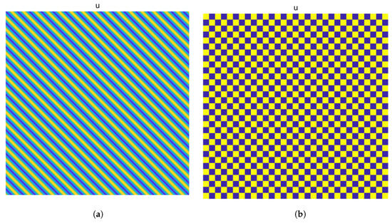
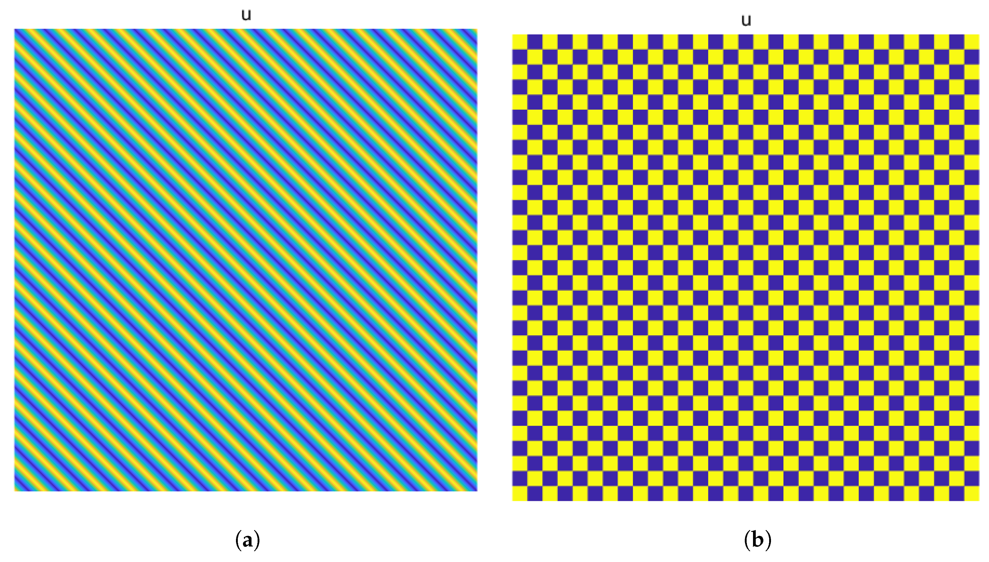
Figure 3. Stripe pattern and hexagon pattern of model (3). (a) Stripe pattern of v. (b) Hexagon pattern of v.

According to [33], if the diffusion index is different, the hexagonal pattern will turn into a square pattern under certain conditions. Therefore, the numerical simulation results indicate that under this set of parameters, the solution of the system conforms to both the condition $\mu <{\mu }_3$ for stripe patterns and the condition $\mu <{\mu }_4$ for hexagonal patterns. In Matlab, color interpolation is applied to enhance coloring and smooth out color transitions, and the hexagonal pattern becomes a stripe pattern, as shown in Figure 3. This also proves the correctness of our theory.

We select the following initial conditions at equilibrium point $E_1=\left(\frac{A}{L},0\right)$:

$$\begin{array}{c}\hfill u\left(x,y,0\right)=\left\{\begin{array}{c}0.5,\hfill \\ 1,other,\hfill \end{array}\right.v\left(x,y,0\right)=\left\{\begin{array}{c}0.25,\hfill \\ 0,other.\hfill \end{array}\right.\end{array}$$

(75)

where

$$\begin{array}{c}\hfill x,y\in [\frac{K}{2}-80:\frac{K}{2}-48,\frac{K}{2}-16:\frac{K}{2}+16]\cup [\frac{K}{2}+48:\frac{K}{2}+80,\frac{K}{2}-16:\frac{K}{2}+16]\end{array}$$

(76)

$$\begin{array}{c}\hfill \cup [\frac{K}{2}-16:\frac{K}{2}+16,\frac{K}{2}-80:\frac{K}{2}-48]\cup [\frac{K}{2}-16:\frac{K}{2}+16,\frac{K}{2}+48:\frac{K}{2}+80]\end{array}$$

(77)

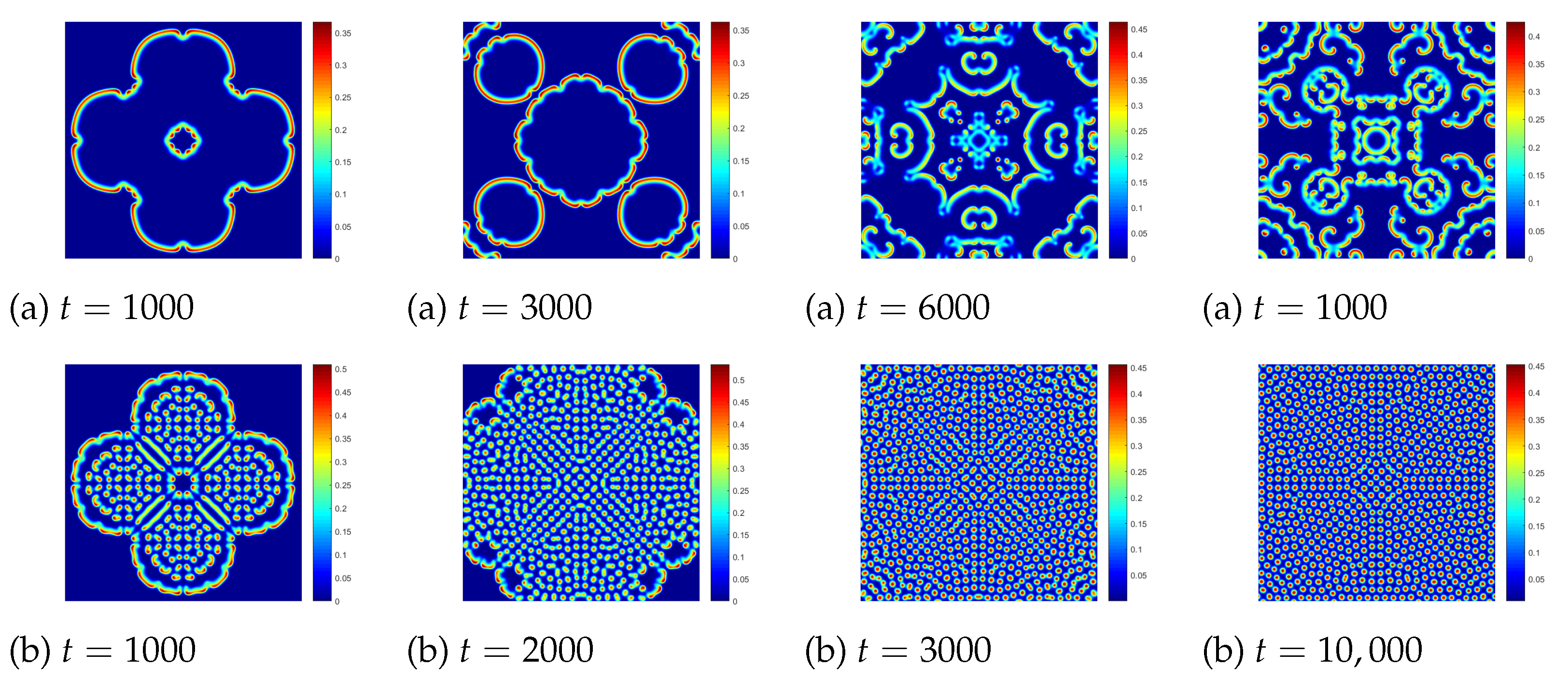
Figure 4 shows the vegetation pattern succession at $d_1=2\times {10}^{-5}$ and $d_1=5\times {10}^{-5}$. The blue area in the picture represents exposed soil, while the red area represents a highly concentrated area of vegetation. In Figure 4a, as t gradually increases, we ultimately find that spot patterns and bars coexist throughout the entire region. Increasing the diffusion rate of surface water, in Figure 4b, we find that as t gradually increases, the stripes decrease prematurely to non-existence, and only the spots remain.

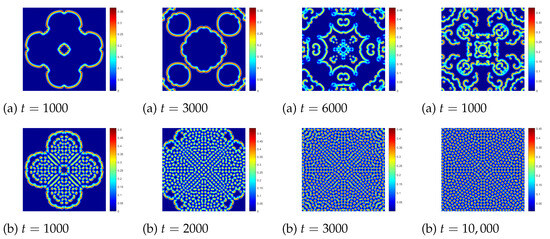
Figure 4. Vegetation distribution pattern in model (3) with different parameters, $d_1$, (a) $d_1=2\times {10}^{-5}$, (b) $d_1=5\times {10}^{-5}$.

Figure 5 shows the vegetation pattern succession with a fractional order $\beta$ of change. As $\beta$ decreases, the vegetation pattern gradually becomes less easily broken and the vegetation density significantly increases. When $\beta =2$, as t gradually increases, the region mainly exists as a bar pattern. Continuously reducing $\beta$, we find that speckle patterns and stripes coexist throughout the entire region.

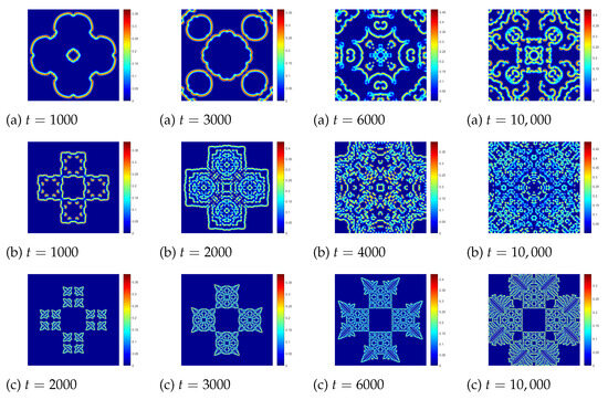
Figure 5. Vegetation distribution pattern in model (3) with different parameters, $\beta$, (a) $\beta =2$, (b) $\beta =1.8$, (c) $\beta =1.6$.

7. Conclusions

In this paper, the vegetation pattern under a semi-arid system of a fractional vegetation–water model in an arid flat environment is studied. We discuss the stability of the positive equilibrium point and study the Hopf bifurcation around the equilibrium point of the fractional parameter, $\alpha$. Through the weak nonlinear analysis method, the mode selection of the vegetation model is given. Through this paper, it can be found that the vegetation in the arid flat environment has a rich pattern structure, including spots, mixing, and stripes. When the diffusion coefficient, d, changes, and other parameters remain unchanged, the pattern structure changes from stripes to spots. When the fractional order parameter, $\beta$, changes and other parameters remain unchanged, the pattern structure becomes more stable and is not easy to destroy. Some novel fractal patterns of fractional vegetation–water models in arid flat environments are shown.

References

- U. Nations. Transforming Our World: The 2030 Agenda for Sustainable Development. 2015. Available online: https://sustainabledevelopment.un.org (accessed on 19 March 2024).
- Lefever, R.; Lejeune, O. On the origin of tiger bush. Bull. Math. Biol. 1997, 59, 263–294. [Google Scholar] [CrossRef]
- Biederman, J.A.; Scott, R.L.; Arnone, J.A., III; Jasoni, R.L.; Litvak, M.E.; Moreo, M.T.; Vivoni, E.R. Shrubland carbon sink depends upon winter water availability in the warm deserts of North America. Agric. For. Meteorol. 2018, 249, 407–419. [Google Scholar] [CrossRef]
- Sun, G.; Wang, C.; Chang, L.; Wu, Y.; Li, L.; Jin, Z. Effects of feedback regulation on vegetation patterns in semi-arid environments. Appl. Math. Model. 2018, 61, 200–215. [Google Scholar] [CrossRef]
- Guo, G.; Qin, Q.; Pang, D.; Su, Y. Positive steady-state solutions for a vegetation-water model with saturated water absorption. Commun. Nonlinear Sci. Numer. Simul. 2024, 131, 107802. [Google Scholar] [CrossRef]
- Scheffer, M.; Bascompte, J.; Brock, W.A.; Brovkin, V.; Carpenter, S.R.; Dakos, V.; Sugihara, G. Early-warning signals for critical transitions. Nature 2009, 461, 53–59. [Google Scholar] [CrossRef]
- Sewalt, L.; Doelman, A. Spatially periodic multipulse patterns in a generalized Klausmeier-Gray-Scott model. Siam J. Appl. Dyn. Syst. 2017, 16, 1113–1163. [Google Scholar] [CrossRef]
- Klausmeier, C.A. Regular and irregular patterns in semiarid vegetation. Science 1999, 284, 1826–1828. [Google Scholar] [CrossRef]
- Wang, X.; Shi, J.; Zhang, G. Bifurcation and pattern formation in diffusive Klausmeier-Gray-Scott model of water-plant interaction. J. Math. Anal. Appl. 2021, 497, 124860. [Google Scholar] [CrossRef]
- Kealy, B.J.; Wollkind, D.J. A nonlinear stability analysis of vegetative Turing pattern formation for an interaction-diffusion plant-surface water model system in an arid flat environment. Bull. Math. Biol. 2012, 74, 803–833. [Google Scholar] [CrossRef]
- Sun, G.; Li, L.; Zhang, Z.K. Spatial dynamics of a vegetation model in an arid flat environment. Nonlinear Dyn. 2013, 73, 2207–2219. [Google Scholar] [CrossRef]
- Guo, G.; Wang, J. Pattern formation and qualitative analysis for a vegetation-water model with diffusion. Nonlinear Anal. Real World Appl. 2024, 76, 104008. [Google Scholar] [CrossRef]
- Gray, P.; Scott, S.K. Autocatalytic reactions in the isothermal, continuous stirred tank reactor: Isolas and other forms of multistability. Chem. Eng. Sci. 1983, 38, 29–43. [Google Scholar] [CrossRef]
- Gray, P.; Scott, S.K. Sustained oscillations and other exotic patterns of behavior in isothermal reactions. J. Phys. Chem. 1985, 89, 22–32. [Google Scholar] [CrossRef]
- Han, C.; Wang, Y.; Li, Z. Novel patterns in a class of fractional reaction-diffusion models with the Riesz fractional derivative. Math. Comput. Simul. 2022, 202, 149–163. [Google Scholar]
- Han, C.; Wang, Y.; Li, Z. A high-precision numerical approach to solving space fractional Gray-Scott model. Appl. Math. Lett. 2022, 125, 107759. [Google Scholar] [CrossRef]
- Liu, Y.; Fan, E.; Yin, B.; Li, H.; Wang, J. TT-M finite element algorithm for a two-dimensional space fractional Gray-Scott model. Comput. Math. Appl. 2020, 80, 1793–1809. [Google Scholar] [CrossRef]
- Zhai, S.; Weng, Z.; Zhuang, Q.; Liu, F.; Anh, V. An effective operator splitting method based on spectral deferred correction for the fractional Gray-Scott model. J. Comput. Appl. Math. 2023, 425, 114959. [Google Scholar] [CrossRef]
- Ning, J.; Wang, Y. Fourier spectral method for solving fractional-in-space variable coefficient KdV-Burgers equation. Indian J. Phys. 2024, 98, 1727–1744. [Google Scholar] [CrossRef]
- Gao, X.; Wang, Y.; Li, Z. Research chaotic dynamic behavior of a fractional-order financial systems with constant inelastic demand. Int. J. Bifurc. Chaos 2024. [Google Scholar]
- Li, Z.; Chen, Q.; Wang, Y.; Li, X. Solving two-sided fractional super-diffusive partial differential equations with variable coefficients in a class of new reproducing kernel spaces. Fractal Fract. 2022, 6, 492. [Google Scholar] [CrossRef]
- Odibat, Z.M.; Shawagfeh, N.T. Generalized Taylor’s formula. Appl. Math. Comput. 2007, 186, 286–293. [Google Scholar] [CrossRef]
- Atangana, A.; Koca, I. Chaos in a simple nonlinear system with Atangana-Baleanu derivatives with fractional order. Chaos Solitons Fractals 2016, 89, 447–454. [Google Scholar] [CrossRef]
- Abdeljawad, T. A Lyapunov type inequality for fractional operators with nonsingular Mittag-Leffler kernel. J. Inequalities Appl. 2017, 2017, 130. [Google Scholar] [CrossRef] [PubMed]
- Lin, X.; Wang, Y.; Wang, J.; Zeng, W. Dynamic analysis and adaptive modified projective synchronization for systems with Atangana-Baleanu-Caputo derivative: A financial model with nonconstant demand elasticity. Chaos Solitons Fractals 2022, 160, 112269. [Google Scholar] [CrossRef]
- Baisad, K.; Moonchai, S. Analysis of stability and Hopf bifurcation in a fractional Gauss-type predator-prey model with Allee effect and Holling type-III functional response. Adv. Differ. Equations 2018, 2018, 82. [Google Scholar] [CrossRef]
- Petráš, I. Fractional-Order Nonlinear Systems: Modeling, Analysis and Simulation; Springer Science & Business Media: Berlin/Heidelberg, Germany, 2011. [Google Scholar]
- Deng, W.; Lü, J. Generating multi-directional multi-scroll chaotic attractors via a fractional differential hysteresis system. Phys. Lett. A 2007, 369, 438–443. [Google Scholar] [CrossRef]
- Ghosh, U.; Pal, S.; Banerjee, M. Memory effect on Bazykin’s prey-predator model: Stability and bifurcation analysis. Chaos Solitons Fractals 2021, 143, 110531. [Google Scholar] [CrossRef]
- Barman, D.; Roy, J.; Alrabaiah, H.; Panja, P.; Mondal, S.P.; Alam, S. Impact of predator incited fear and prey refuge in a fractional order prey predator model. Chaos Solitons Fractals 2021, 142, 110420. [Google Scholar] [CrossRef]
- Balci, E. Predation fear and its carry-over effect in a fractional order prey-predator model with prey refuge. Chaos Solitons Fractals 2023, 175, 114016. [Google Scholar] [CrossRef]
- Diethelm, K.; Ford, N.J.; Freed, A.D. A predictor-corrector approach for the numerical solution of fractional differential equations. Nonlinear Dyn. 2002, 29, 3–22. [Google Scholar] [CrossRef]
- Zhang, L.; Tian, C. Turing pattern dynamics in an activator-inhibitor system with superdiffusion. Phys. Rev. E 2014, 90, 062915. [Google Scholar] [CrossRef] [PubMed]
Disclaimer/Publisher’s Note: The statements, opinions and data contained in all publications are solely those of the individual author(s) and contributor(s) and not of MDPI and/or the editor(s). MDPI and/or the editor(s) disclaim responsibility for any injury to people or property resulting from any ideas, methods, instructions or products referred to in the content. |
© 2024 by the authors. Licensee MDPI, Basel, Switzerland. This article is an open access article distributed under the terms and conditions of the Creative Commons Attribution (CC BY) license (https://creativecommons.org/licenses/by/4.0/).