A Preconditioned Policy–Krylov Subspace Method for Fractional Partial Integro-Differential HJB Equations in Finance

Abstract

To better simulate the prices of underlying assets and improve the accuracy of pricing financial derivatives, an increasing number of new models are being proposed. Among them, the Lévy process with jumps has received increasing attention because of its capacity to model sudden movements in asset prices. This paper explores the Hamilton–Jacobi–Bellman (HJB) equation with a fractional derivative and an integro-differential operator, which arise in the valuation of American options and stock loans based on the Lévy-$\alpha$-stable process with jumps model. We design a fast solution strategy that includes the policy iteration method, Krylov subspace method, and banded preconditioner, aiming to solve this equation rapidly. To solve the resulting HJB equation, a finite difference method including an upwind scheme, shifted Grünwald approximation, and trapezoidal method is developed with stability and convergence analysis. Then, an algorithmic framework involving the policy iteration method and the Krylov subspace method is employed. To improve the performance of the above solver, a banded preconditioner is proposed with condition number analysis. Finally, two examples, sugar option pricing and stock loan valuation, are provided to illustrate the effectiveness of the considered model and the efficiency of the proposed preconditioned policy–Krylov subspace method.

1. Introduction

The option-pricing problem has always been a hot research topic in finance, as options are important tools for investment and hedging risk. Among a variety of option products, American options have gained popularity in the market because they can be exercised before maturity. This feature makes them the predominant type of options sold in the market. Concurrently, stock loans have become commonplace in the current financial market, and determining how much money can be loaned against the current value of stocks has also emerged as a significant area of research. Given that both of these financial instruments can be exercised (or repaid) at any time, their prices (or loan amounts) can be determined by solving the following linear complementarity problem (LCP):

$$\left\{\begin{array}{c}\mathcal{L}U(x,t)\ge 0,\hfill \\ U(x,t)\ge U^{\ast }(x,t),\hfill \\ \mathcal{L}U(x,t)[U(x,t)-U^{\ast }(x,t)]=0,\hfill \end{array}\right.$$

(1)

where $\mathcal{L}$ is a linear operator containing partial derivatives, $U(x,t)$ represents the value, and $U^{\ast }(x,t)$ signifies the constraint.

To solve the LCP (1), it is necessary to understand the definition of the operator $\mathcal{L}$, which depends on the assumed underlying asset price behavior. According to the well-known Black–Scholes model [1], the underlying asset price is modeled as follows:

$$d{S}_t=\nu S_{t}dt+\sigma S_{t}d{W}_t,$$

where $S_t$ is the assets’ price, $W_t$ represents the standard Brownian motion, $\nu$ is the drift rate of the asset’s return, and:

$$\mathcal{L}U(S,t):=-\frac{\partial U(S,t)}{\partial t}-\frac{1}{2}{\sigma }^2{S}^2\frac{{\partial }^{2}U(S,t)}{\partial S^2}-rS\frac{\partial U(S,t)}{\partial S}+rU(S,t),$$

with r being the interest rate, $\sigma$ being the volatility, and S being the asset’s price. However, this model cannot account for many empirical observations of asset prices, such as sudden price movements. Hence, new models have been proposed to handle these issues, including stochastic volatility models [2,3], jump diffusion models [4], self-exciting jump models [5], Hawkes jump diffusion models [6], mixed fractional Brownian model [7], two-factor non-affine stochastic volatility model [8], and sub-fractional Brownian model [9,10]. The model based on the Lévy process, notable for its ability to model price jumps and transform into a fractional diffusion equation [11], is among these. With different density functions, different models have been proposed, such as the KoBoL model [12], the CGMY model [13], and the FMLS model [14]. The Lévy process with jumps has also been proposed to more accurately describe the price of underlying assets [15,16]. In this paper, this stochastic process is used to model the underlying assets, defined by

$$d{x}_t=(r-\nu -\tilde{\lambda }\xi )dt+\sigma d{L}_t^{\alpha ,-1}+d(\sum _{i=1}^{N_t}{Y}_i),$$

where $x_t=ln{S}_t$ and t denotes the current time, with $\nu =-\frac{1}{2}{\sigma }^{\alpha }sec\left(\frac{\alpha \pi }{2}\right)$ being the convexity adjustment. The variable $L_t^{\alpha ,-1}$ represents the Lévy-$\alpha$-stable process with maximum skewness, where the tail index $\alpha$ falls within the range of (1, 2). $N_t$ denotes a Poisson process characterized by the jump intensity $\tilde{\lambda }\ge 0$. $\left\{Y_i,i=1,2\cdots \right\}$ is a sequence of independent and identically distributed random variables, and $\xi =e^{u_J+\frac{{\sigma }_J^2}{2}}-1$, where the parameters $u_J$ and ${\sigma }_J$ represent the expectation and standard deviation of the jumps, respectively. Then, the operator $\mathcal{L}U(x,t)$ includes both a fractional derivative and an integral operator (for more details, refer to the following section). By solving the LCP in (1) with this $\mathcal{L}U(x,t)$ under specific boundary and initial conditions, we can determine the price of American options or the value of stock loans.

To address the LCP arising from the valuation of American options and stock loans, various numerical algorithms have been developed. These can be categorized into five primary strategies. The first focuses on identifying the optimal execution boundary to resolve the challenges, as demonstrated by the approach presented in [17]. The second strategy transforms the problem into a linear framework through either semi-implicit or implicit–explicit schemes, such as the L-stable method [18], the linearly implicit predictor–corrector scheme [19], and the IMEX BDF method [20]. The third approach converts the problem into a nonlinear equation, utilizing iterative methods for solution acquisition, including the fixed-point method [21], the preconditioned penalty method [22], and the modulus-based matrix splitting iteration method [23]. The fourth approach involves devising iterative methods for direct LCP resolution, exemplified by the projected SOR method [24] and the projected algebraic multigrid method [25]. The last category of algorithms consists of the recently popular deep learning algorithms, such as the neural network method [26] and the physics-informed neural network method [27]. For the LCP discussed in this paper, a Laplace transform method is introduced for rapid resolution by avoiding time marching [15]. Moreover, a fast solution strategy that combines Newton’s method with the preconditioned conjugate gradient normal residual method is proposed in [16], benefiting from fast Fourier transformation acceleration and achieving an operational cost of $\mathcal{O}(NlogN)$ per inner iteration. This paper introduces an alternative approach, translating the LCP into a Hamilton–Jacobi–Bellman (HJB) equation, and devising a fast algorithm for its resolution, complete with theoretical assurances.

This study aims to devise a fast algorithm for solving the HJB equation, which includes a fractional derivative and an integral operator derived from the LCP based on the Lévy-$\alpha$-stable process with jumps model. To tackle this equation, a nonlinear finite difference method is developed, accompanied by stability and convergence analyses. Subsequently, the policy iteration method and the Krylov subspace method are applied to solve the resultant finite difference scheme. A banded preconditioner is also proposed to enhance the convergence speed of the internal iterative method, supported by theoretical analysis. These steps enable the development of a preconditioned policy–Krylov subspace method for solving the fractional partial integro-differential HJB equations in finance, ensuring an efficient and theoretically sound solution.

The rest of this article is organized as follows: The description of the equation considered in this paper is illustrated in Section 2. A nonlinear finite difference scheme is proposed in Section 3 to discretize the HJB equation with the unconditional stability guarantee and first-order convergence rate. In Section 4, a fast algorithm framework incorporating the policy iteration method and the Krylov subspace method is introduced. In Section 5, a banded preconditioner is proposed with theoretical analysis about the condition number of the preconditioned matrix. Numerical experiments are given in Section 6, and conclusions are drawn in Section 7.

2. Description of the Equation

As described in Section 1, the price of the American options and the stock loans can be obtained by solving the LCP in (1). Referring to [28], solving the LCP can be achieved by converting it into an HJB equation. Then the pricing model based on the Lévy-$\alpha$-stable process with jumps considered in this paper can be solved by solving the following HJB equation, which is defined as follows:

$$\left\{\begin{array}{c}min\{\mathcal{L}U(x,t),U(x,t)-U^{\ast }(x,t)\}=0,(x,t)\in (x_L,x_R)\times [0,T),\hfill \\ U(x,T)=\Psi (x,T),x\in (x_L,x_R),\hfill \\ U(x_L,t)=\Psi (x_L,t),U(x_R,t)=\Psi (x_R,t),t\in [0,T],\hfill \end{array}\right.$$

(2)

where $x=lnS$, and S is the asset’s price. In the above equation, $\mathcal{L}U(x,t)$ is defined by

$$\begin{array}{c}\hfill \mathcal{L}U(x,t):=-\frac{\partial U(x,t)}{\partial t}-(r-\nu -\tilde{\lambda }\xi )\frac{\partial U(x,t)}{\partial x}-\nu D_{-}^{\alpha }U(x,t)\\ \hfill +(r+\tilde{\lambda })U(x,t)-\tilde{\lambda }{\int }_{-\infty }^{+\infty }U(x+y,t)f\left(y\right)dy,\end{array}$$

(3)

where $D_{-}^{\alpha }U(x,t)$ is the left Riemann–Liouville fractional derivative [29], and the definition of the parameters r, $\nu$, $\tilde{\lambda }$, $\xi$ has been given in Section 1. The boundary conditions and initial condition are determined by the function $\Psi (x,t)$, which has different meanings in different problems. This paper considers the problems of pricing American options and stock loans; hence, the definition of $\Psi (x,t)$ is given as follows:

$$\Psi (x,t)=\left\{\begin{array}{c}max(0,e^x-K),\mathrm{for}\mathrm{American}\mathrm{option}\mathrm{pricing},\hfill \\ max\{0,e^x-K{e}^{\gamma t}\},\mathrm{for}\mathrm{stock}\mathrm{loan}\mathrm{pricing},\hfill \end{array}\right.$$

for $x\in (-\infty ,\infty )$ and $t\in [0,T]$. For the American option pricing, K is the strike price. For stock loan pricing, K is the principal value, and $\gamma$ is the interest rate of the loan [30]. Additionally, $U(z,t)=\Psi (z,t)$ for $z\in (-\infty ,x_L)\cup (x_R,\infty )$ in (3).

The main difficulty in solving the HJB Equation (2), apart from it being a nonlinear equation, also lies in how to handle the Riemann–Liouville fractional derivative and the integral operator. First is the Riemann–Liouville fractional derivative, which is defined as follows:

$$D_{-}^{\alpha }U(x,t)=\frac{1}{\Gamma (2-\alpha )}\frac{{\partial }^2}{\partial x^2}{\int }_{-\infty }^x\frac{U(\zeta ,t)}{{(x-\zeta )}^{\alpha -1}}d\zeta .$$

Because it is a global operator, using the shifted Grünwald approximation [29] will result in a dense coefficient matrix after discretization, thus making the solution challenging.

On the other hand, the integro-differential part ${\int }_{-\infty }^{+\infty }U(x+y,t)f\left(y\right)dy$ also poses computational difficulties. If the trapezoidal method is used for discretization [15], it will also result in a dense coefficient matrix. Therefore, in summary, when designing a fast algorithm to solve the HJB equation, it is necessary to address the computational challenges posed by a fractional derivative and an integro-differential operator. In addition, differing from Refs. [15,16], the probability density function $f\left(z\right)$ of $Y_i$ is described by the following Gaussian distribution formula [31]:

$$f\left(z\right)=\frac{e^{-{(z-u_J)}^2/2{\sigma }_J^2}}{\sqrt{2\pi }{\sigma }_J}.$$

3. Finite Difference Method with Theoretical Analysis

As mentioned above, since $\mathcal{L}U(x,t)$ in the HJB Equation (2) involves both a fractional derivative and an integral operator, finding the analytical solution to the HJB equation is challenging. Consequently, numerical methods become the primary approach for solving the aforementioned HJB equation. In this section, a finite difference method is developed to discretize the equation, which includes the shifted Grünwald approximation, an upwind scheme and the trapezoidal formulas.

3.1. Finite Difference Method

Let N and M be positive integers. Divide the spatial interval $[x_L,x_R]$ and temporal interval $[0,T]$ into $N+1$ and M sub-intervals, respectively. That is,

$$\begin{array}{ccc}\hfill x_i& =& x_L+ih,\mathrm{for}i=0,1,\dots ,N+1,\hfill \\ \hfill t_m& =& T+m\tau ,\mathrm{for}m=0,1,\dots ,M,\hfill \end{array}$$

where $h=\frac{x_R-x_L}{N+1}$, $\tau =-T/M$. With above finite difference mesh, the left fractional derivative $D_{-}^{\alpha }U(x,t)$ can be discretized using the shifted Grünwald approximation [29], expressed as

$$D_{-}^{\alpha }U(x_i,t_m)=\frac{1}{h^{\alpha }}\sum _{k=0}^{i+1}{g}_k^{\left(\alpha \right)}U(x_{i-k+1},t_m)+\mathcal{O}\left(h\right),$$

(4)

for all $1<\alpha <2$. The sequence $\left\{g_k^{\left(\alpha \right)}\right\}$ is defined by

$$\left\{\begin{array}{c}{g}_0^{\left(\alpha \right)}=1,\hfill \\ g_k^{\left(\alpha \right)}=\frac{{(-1)}^k}{k!}\alpha (\alpha -1)\cdots (\alpha -k+1),\hfill & \hfill \mathrm{for}k=1,2,3\dots .\end{array}\right.$$

(5)

For the advection term, the upwind scheme [32] is applied, as given by

$$\frac{\partial U(x_i,t_m)}{\partial x}=\left\{\begin{array}{c}\frac{U(x_i+h,t_m)-U(x_i,t_m)}{h}+\mathcal{O}\left(h\right),ifr-\nu -\tilde{\lambda }\xi \ge 0,\hfill \\ \frac{U(x_i,t_m)-U(x_i-h,t_m)}{h}+\mathcal{O}\left(h\right),ifr-\nu -\tilde{\lambda }\xi <0.\hfill \end{array}\right.$$

(6)

In addition, the integral part in (3) can be approximated by the trapezoidal formulas. To simplify the notation, we denote $\Omega (\widehat{u},\widehat{\sigma },x)$ as

$$\Omega (\widehat{u},\widehat{\sigma },x)=1-F\left(x\right)={\int }_x^{+\infty }\frac{e^{-{(z-\widehat{u})}^2/2{\widehat{\sigma }}^2}}{\sqrt{2\pi }\widehat{\sigma }}dz,$$

(7)

where $F\left(x\right)={\int }_{-\infty }^x\frac{e^{-{(z-\widehat{u})}^2/2{\widehat{\sigma }}^2}}{\sqrt{2\pi }\widehat{\sigma }}dz$ denotes the cumulative distribution function with expectation $\widehat{u}$ and standard deviation $\widehat{\sigma }$, evaluated at the values in x.

To simplify the analysis, we assume that the truncation domain is sufficiently large; i.e., the left and right boundary conditions for the American call option are 0 and $e^x-K$, respectively. As mentioned before, the value outside the domain satisfies that $U(z,t)=\Psi (z,t)$ for $z\in (-\infty ,x_L)\cup (x_R,\infty )$. Similar to the approach in [33], with the notation given in (7), when $x=x_i$, we have

$$\begin{array}{cc}\hfill & {\int }_{-\infty }^{+\infty }U(x_i+z,t_m)f\left(z\right)dz\hfill \\ \hfill =& {\int }_{-\infty }^{x_0-x_i}U(x_i+z,t_m)f\left(z\right)dz+{\int }_{x_0-x_i}^{x_{N+1}-x_i}U(x_i+z,t_m)f\left(z\right)dz\hfill \\ \hfill & +{\int }_{x_{N+1}-x_i}^{+\infty }U(x_i+z,t_m)f\left(z\right)dz\hfill \\ \hfill =& {\int }_{-\infty }^{x_0-x_i}U(x_i+z,t_m)f\left(z\right)dz+\sum _{j=0}^N{\int }_{x_j-x_i}^{x_{j+1}-x_i}U(x_i+z,t_m)f\left(z\right)dz\hfill \\ \hfill & +{\int }_{x_{N+1}-x_i}^{+\infty }U(x_i+z,t_m)f\left(z\right)dz\hfill \\ \hfill =& \sum _{j=0}^N\frac{1}{2}[U(x_j,t_m)+U(x_{j+1},t_m)]{\int }_{(j-i)h}^{(j-i+1)h}f\left(z\right)dz+{\eta }_i+\mathcal{O}\left(h^2\right)\hfill \\ \hfill =& \sum _{j=0}^N{\rho }_{j-i}[U(x_j,t_m)+U(x_{j+1},t_m)]+{\eta }_i+\mathcal{O}\left(h^2\right),\hfill \end{array}$$

(8)

and define ${\rho }_j$ as follows,

$$\begin{array}{c}\hfill {\rho }_j=\frac{1}{2}{\int }_{jh}^{(j+1)h}f\left(z\right)dz=\frac{1}{2}{\int }_{jh}^{(j+1)h}\frac{e^{-{(z-u_J)}^2/2{\sigma }_J^2}}{\sqrt{2\pi }{\sigma }_J}dz,\\ \hfill =\frac{1}{2}\Omega (u_J,{\sigma }_J,jh)-\frac{1}{2}\Omega (u_J,{\sigma }_J,(j+1)h).\end{array}$$

(9)

Additionally, ${\eta }_i$ varies based on the financial product in question. For the American option pricing, ${\eta }_i$ is defined as follows:

$$\begin{array}{cc}\hfill {\eta }_i& ={\int }_{x_{N+1}-x_i}^{+\infty }(e^{x_i+z}-K)f\left(z\right)dz={\int }_{x_{N+1}-x_i}^{+\infty }(e^{x_i+z}-K)\frac{e^{-{(z-u_J)}^2/2{\sigma }_J^2}}{\sqrt{2\pi }{\sigma }_J}dz\hfill \\ \hfill & =e^{\frac{{\sigma }_J^2+2u_J+2x_i}{2}}{\int }_{x_{N+1}-x_i}^{+\infty }\frac{e^{-{(z-(u_J+{\sigma }_J^2))}^2/2{\sigma }_J^2}}{\sqrt{2\pi }{\sigma }_J}dz-K{\int }_{x_{N+1}-x_i}^{+\infty }\frac{e^{-{(z-u_J)}^2/2{\sigma }_J^2}}{\sqrt{2\pi }{\sigma }_J}dz\hfill \\ \hfill & =e^{\frac{{\sigma }_J^2+2u_J+2x_i}{2}}\Omega (u_J+{\sigma }_J^2,{\sigma }_J,x_{N+1}-x_i)-K\Omega (u_J,{\sigma }_J,x_{N+1}-x_i).\hfill \end{array}$$

(10)

Similarly, by assuming that the truncation domain for the stock loan is sufficiently large, then the left and right boundary conditions are set to 0 and $e^x-K{e}^{\gamma t}$, respectively. Thus, the operator ${\int }_{-\infty }^{+\infty }U(x_i+z,t_m)f\left(z\right)dz$, used in the stock loan pricing, can be discretized according to (8), and ${\eta }_i$ is given by

$${\eta }_i=e^{\frac{{\sigma }_J^2+2u_J+2x_i}{2}}\Omega (u_J+{\sigma }_J^2,{\sigma }_J,x_{N+1}-x_i)-K{e}^{\gamma t}\Omega (u_J,{\sigma }_J,x_{N+1}-x_i).$$

Also, denote $c_1=r-\nu -\tilde{\lambda }\xi$, $c_2=\nu$, $c_3=r+\tilde{\lambda }$, $c_4=\tilde{\lambda }$; combining (4), (6) and (8), the HJB Equation (2) can be discretized as

$$min\{\tilde{\mathcal{L}}{u}_i^{m+1},u_i^{m+1}-u_i^{m+1,\ast }\}=0,$$

(11)

where $u_i^m\approx U(x_i,t_m)$, $u_i^{m,\ast }\approx \Psi (x_i,t_m)$,

$$\begin{array}{c}\hfill \tilde{\mathcal{L}}{u}_i^{m+1}=-\frac{u_i^{m+1}-u_i^m}{\tau }-c_1\frac{u_{i+\theta }^{m+1}-u_{i-(1-\theta )}^{m+1}}{h}-\frac{c_2}{h^{\alpha }}\sum _{k=0}^{i+1}{g}_k^{\left(\alpha \right)}{u}_{i-k+1}^{m+1}\\ \hfill +c_3{u}_i^{m+1}-c_4(\sum _{j=0}^N{\rho }_{j-i}[u_j^{m+1}+u_{j+1}^{m+1}]+{\eta }_i),\end{array}$$

(12)

and

$$\theta =\left\{\begin{array}{c}1,\mathrm{if}{c}_1\ge 0,\hfill \\ 0,\mathrm{if}{c}_1<0.\hfill \end{array}\right.$$

3.2. Matrix Form

To simplify the notation of the matrix form, we use $T_n$ to denote an n-by-n Toeplitz matrix, which is defined by

$$T_n(t_{n-1},\dots ,t_1;t_0;t_{-1},\dots ,t_{1-n})=\left[\begin{array}{ccccc}{t}_0& t_{-1}& \cdots & t_{2-n}& t_{1-n}\\ t_1& t_0& t_{-1}& \cdots & t_{2-n}\\ ⋮& t_1& t_0& \ddots & ⋮\\ t_{n-2}& \cdots & \ddots & \ddots & t_{-1}\\ t_{n-1}& t_{n-2}& \cdots & t_1& t_0\end{array}\right].$$

Define the vectors $u^m={[u_1^m,u_2^m,u_3^m,\dots ,u_N^m]}^T$, $u^{m,\ast }={[u_1^{m,\ast },u_2^{m,\ast },u_3^{m,\ast },\dots ,u_N^{m,\ast }]}^T$, $f^m={[f_1^m,f_2^m,f_3^m,\dots ,f_N^m]}^T$. Since $\tau <0$, $\tilde{\mathcal{L}}{u}_i^{m+1}\ge 0$ is equal to $-\tau \tilde{\mathcal{L}}{u}_i^{m+1}\ge 0$. Then, the matrix form of the numerical scheme (11) can be written as

$$min\{W{u}^{m+1}-u^m+\tau f^{m+1},u^{m+1}-u^{m+1,\ast }\}=0,$$

(13)

where

$$W=(1-\tau c_3)I_N+\frac{\tau c_1}{h}D+\frac{\tau c_2}{h^{\alpha }}G+\tau c_{4}S,$$

(14)

and $I_N$ is an N by N identity matrix; other matrices in (14) can be expressed by

$$\begin{array}{cc}\hfill & D=T_n(0,0,\dots ,\theta -1;1-2\theta ;\theta ,0,\dots ,0),\hfill \\ \hfill & G=T_n(g_n^{\left(\alpha \right)},g_{n-1}^{\left(\alpha \right)},\dots ,g_2^{\left(\alpha \right)};g_1^{\left(\alpha \right)};g_0^{\left(\alpha \right)},0,0\dots ,0),\hfill \\ \hfill & S=T_n(s_{1-N},s_{2-N},\dots ,s_{-1};s_0;s_1,s_2,\dots ,s_{N-1}),\hfill \end{array}$$

where

$$s_j=\frac{1}{2}{\int }_{(j-1)h}^{(j+1)h}f\left(z\right)dz=\frac{1}{2}{\int }_{(j-1)h}^{(j+1)h}\frac{e^{\frac{-{(z-\mu )}^2}{2{\sigma }^2}}}{\sqrt{2\pi }{\sigma }_J}dz=\frac{1}{2}\Omega (u_J,{\sigma }_J,(j-1)h)-\frac{1}{2}\Omega (u_J,{\sigma }_J,(j+1)h).$$

To simplify the notation, we assume that the truncation domain is large, then the specific form of the entry $f_i^m$ is given as follows:

$$f_i^m=\left\{\begin{array}{c}{c}_4({\eta }_i+{\rho }_{N-i}{u}_{N+1}^{m+1}),ifi=1,2,\cdots ,N-1,\hfill \\ c_4({\eta }_N+{\rho }_0{u}_{N+1}^{m+1})+\frac{c_2}{h^{\alpha }}{u}_{N+1}^{m+1}+\frac{c_1}{h}{u}_{N+1}^{m+1},ifi=Nand{c}_1\ge 0,\hfill \\ c_4({\eta }_N+{\rho }_0{u}_{N+1}^{m+1})+\frac{c_2}{h^{\alpha }}{u}_{N+1}^{m+1},ifi=Nand{c}_1<0.\hfill \end{array}\right.$$

3.3. Stability and Convergence Analysis

Although the numerical scheme has been developed, theorems about the stability and convergence are still needed to ensure the numerical solution can be obtained correctly. For theoretical analysis, the following proposition is introduced.

Proposition 1

([34]). The sequence $\left\{g_k^{\left(\alpha \right)}\right\}$ defined in (5) has the following properties:

$$\left\{\begin{array}{c}{g}_0^{\left(\alpha \right)}=1,g_1^{\left(\alpha \right)}=-\alpha <0,g_2^{\left(\alpha \right)}>g_3^{\left(\alpha \right)}>g_4^{\left(\alpha \right)}>\cdots >0,\hfill \\ \sum _{k=0}^{\infty }{g}_k^{\left(\alpha \right)}=0,\sum _{k=0}^n{g}_k^{\left(\alpha \right)}<0,\forall n\ge 1.\hfill \end{array}\right.$$

The above proposition provides the properties of the shifted Grünwald approximation. Additionally, one more lemma is needed to analyze the properties of the integral operator, which is given as follows:

Lemma 1.

With the density function $f\left(z\right)$, the entries of the matrix S satisfy

$$0<\sum _{1-N}^{N-1}{s}_j<1.$$

Proof. 

By the definition of $s_j$, we have

$$\begin{array}{cc}\hfill \sum _{1-N}^{N-1}{s}_j=& \frac{1}{2}\sum _{j=1-N}^{N-1}\left({\int }_{(j-1)h}^{jh}\frac{e^{\frac{-{(z-\mu )}^2}{2{\sigma }^2}}}{\sqrt{2\pi }{\sigma }_J}dz+{\int }_{jh}^{(j+1)h}\frac{e^{\frac{-{(z-\mu )}^2}{2{\sigma }^2}}}{\sqrt{2\pi }{\sigma }_J}dz\right)\hfill \\ \hfill =& \frac{1}{2}\left({\int }_{-Nh}^{(N-1)h}\frac{e^{\frac{-{(z-\mu )}^2}{2{\sigma }^2}}}{\sqrt{2\pi }{\sigma }_J}dz+{\int }_{(1-N)h}^{Nh}\frac{e^{\frac{-{(z-\mu )}^2}{2{\sigma }^2}}}{\sqrt{2\pi }{\sigma }_J}dz\right)\hfill \\ \hfill <& 1.\hfill \end{array}$$

On the other hand, $s_j$ is equal to the probability of a variable X that follows a normal distribution, in the range of $(j-1)h$ to $(j+1)h$, that is, $Pr\left(\right(j-1)h<X<(j+1\left)h\right)$. Therefore, its value is definitely greater than 0 for all j.    □

In the following analysis, the properties of the $\mathcal{M}$-matrix play an important role. Therefore, the definition of the $\mathcal{M}$-matrix is provided first. A matrix is called an $\mathcal{M}$-matrix if it is a diagonally dominant matrix, with all entries on the main diagonal being positive and all off-diagonal entries being negative [35]. To prove the stability and convergence of the numerical scheme, combining Proposition 1 and Lemma 1, the properties of matrix W are analyzed.

Lemma 2.

For $1<\alpha <2$, the matrix $W={\left[w_{i,j}\right]}_{i,j=1}^N$ is an $\mathcal{M}$-matrix, and satisfies

$$\begin{array}{c}\hfill |w_{i,i}|-\sum _{j=1,j\ne i}^N|w_{i,j}| \ge 1+|\tau |r.\end{array}$$

Proof. 

By the definition of D and G, and with Proposition 1, it is straightforward to understand that the matrices $\frac{\tau c_1}{h}D$ and $\frac{\tau c_2}{h^{\alpha }}G$ are the weakly diagonally dominant matrices which have positive diagonals and non-positive off-diagonals. Let us denote a matrix $\tilde{W}$ as $\tilde{W}=(1-\tau c_3)I_N+\tau c_{4}S$. Then, we obtain that

$$\begin{array}{cc}\hfill |{\tilde{w}}_{i,i}|-\sum _{j=1,j\ne i}^N\left|{\tilde{w}}_{i,j}\right|\ge & 1-\tau c_3+\tau c_4{s}_0-\left|\tau \right|c_4\sum _{j=1-N,j\ne 0}^{N-1}\left|s_j\right|\hfill \\ \hfill =& 1+\left|\tau \right|r+\left|\tau \right|c_4-\left|\tau \right|c_4\sum _{j=1-N}^{N-1}\left|s_j\right|\hfill \\ \hfill \ge & 1+\left|\tau \right|r.\hfill \end{array}$$

and

$$\begin{array}{c}\hfill {\tilde{w}}_{i,j}=\left\{\begin{array}{c}1+\left|\tau \right|r+\left|\tau \right|c_4-\left|\tau \right|c_4{s}_0,fori=j,\hfill \\ \tau c_4{s}_j,fori\ne j.\hfill \end{array}\right.\end{array}$$

(15)

Based on the definition of $\tilde{W}$ in (15), and given that $\tau s_j<0$ and $\left|\tau \right|c_4>\left|\tau \right|c_4{s}_0$, $\tilde{W}$ is a diagonally dominant matrix with positive diagonals and negative off-diagonals. Since the sum of matrices $\tilde{W}$, $\frac{\tau c_1}{h}D$ and $\frac{\tau c_2}{h^{\alpha }}G$ constitutes the matrix W, we know that W is an $\mathcal{M}$-matrix and satisfies $|w_{i,i}|-{\sum }_{j=1,j\ne i}^N|w_{i,j}| \ge 1+|\tau |r$.    □

To prove that the numerical scheme is stable, we assume that $u_i^m$ and ${\tilde{u}}_i^m$ are both the numerical solutions of the scheme (13). Denote that $E_i^m=u_i^m-{\tilde{u}}_i^m$ and the vector $E^m={[E_1^m,E_2^m,\dots ,E_N^m]}^T$, then we have the following theorem.

Theorem 1.

The proposed nonlinear scheme (13) is unconditionally stable, that is,

$$\parallel E^m{\parallel }_{\infty }\le {\parallel E^0\parallel }_{\infty },$$

where $m=1,2,\dots ,M$.

Proof. 

Assume that the $i_0$-th entry of the vector $E^m$ is such that $\parallel E^m{\parallel }_{\infty }=|E_{i_0}^m|=max\{|E_i^m\left|\right\}$ for $i=1,2,\dots ,N$. We can then proceed with the proof as follows: since $u_i^m$ and ${\tilde{u}}_i^m$ are both the numerical solutions of the scheme, we are given the following two equations:

$$\begin{array}{c}\hfill min\{W{u}^m-u^{m-1}+\tau f^m,u^m-u^{m,\ast }\}=0,\\ \hfill min\{W{\tilde{u}}^m-{\tilde{u}}^{m-1}+\tau f^m,{\tilde{u}}^m-u^{m,\ast }\}=0.\end{array}$$

By assuming the existence of the solution, the proof can be discussed in four cases.

Case 1:

Assume that in the $i_0$-th row of the vector $u^m$ and ${\tilde{u}}^m$, two solutions satisfy ${\sum }_{j=1}^N{w}_{i_0,j}{u}_j^m-u_{i_0}^{m-1}+\tau f_{i_0}^m=0$, $u_{i_0}^m\ge u_{i_0}^{m,\ast }$, ${\sum }_{j=1}^N{w}_{i_0,j}{\tilde{u}}_j^m-{\tilde{u}}_{i_0}^{m-1}+\tau f_{i_0}^m=0$, and ${\tilde{u}}_{i_0}^m\ge u_{i_0}^{m,\ast }$. Then we have the following equation:

$$\begin{array}{cc}\hfill \sum _{j=1}^N{w}_{i_0,j}{u}_j^m-u_{i_0}^{m-1}+\tau f_{i_0}^m=& \sum _{j=1}^N{w}_{i_0,j}{\tilde{u}}_j^m-{\tilde{u}}_{i_0}^{m-1}+\tau f_{i_0}^m+\sum _{j=1}^N{w}_{i_0,j}{E}_j^m-E_{i_0}^{m-1}\hfill \\ \hfill =& \sum _{j=1}^N{w}_{i_0,j}{E}_j^m-E_{i_0}^{m-1}.\hfill \end{array}$$

With Lemma 2, this yields

$$\parallel E^m{\parallel }_{\infty }= |E_{i_0}^m| \le |\sum _{j=1}^N{w}_{i_0,j}{E}_j^m| = |E_{i_0}^{m-1}| \le \parallel E^{m-1}{\parallel }_{\infty }.$$

Case 2:

In the $i_0$-th row of the vector $u^m$ and ${\tilde{u}}^m$, two solutions satisfy ${\sum }_{j=1}^N{w}_{i_0,j}{u}_j^m-u_{i_0}^{m-1}+\tau f_{i_0}^m\ge 0$, $u_{i_0}^m=u_{i_0}^{m,\ast }$, ${\sum }_{j=1}^N{w}_{i_0,j}{\tilde{u}}_j^m-{\tilde{u}}_{i_0}^{m-1}+\tau f_{i_0}^m=0$, and ${\tilde{u}}_{i_0}^m\ge u_{i_0}^{m,\ast }$. Then, we have

$$E_{i_0}^m=u_{i_0}^m-{\tilde{u}}_{i_0}^m=u_{i_0}^{m,\ast }-{\tilde{u}}_{i_0}^m\le 0.$$

On the other hand, this leads to

$$\begin{array}{cc}\hfill \sum _{j=1}^N{w}_{i_0,j}{u}_j^m-u_{i_0}^{m-1}+\tau f_{i_0}^m=& \sum _{j=1}^N{w}_{i_0,j}{\tilde{u}}_j^m-{\tilde{u}}_{i_0}^{m-1}+\tau f_{i_0}^m+\sum _{j=1}^N{w}_{i_0,j}{E}_j^m-E_{i_0}^{m-1}\hfill \\ \hfill =& \sum _{j=1}^N{w}_{i_0,j}{E}_j^m-E_{i_0}^{m-1}\ge 0.\hfill \end{array}$$

With Lemma 2, we have

$$E_{i_0}^{m-1}\le \sum _{j=1}^N{w}_{i_0,j}{E}_j^m\le E_{i_0}^m\le 0.$$

Thus,

$$\parallel E^m{\parallel }_{\infty }\le {\parallel E^{m-1}\parallel }_{\infty }.$$

Case 3:

In the $i_0$-th row of the vector $u^m$ and ${\tilde{u}}^m$, two solutions satisfy ${\sum }_{j=1}^N{w}_{i_0,j}{u}_j^m-u_{i_0}^{m-1}+\tau f_{i_0}^m=0$, $u_{i_0}^m\ge u_{i_0}^{m,\ast }$, ${\sum }_{j=1}^N{w}_{i_0,j}{\tilde{u}}_j^m-{\tilde{u}}_{i_0}^{m-1}+\tau f_{i_0}^m\ge 0$, and ${\tilde{u}}_{i_0}^m=u_{i_0}^{m,\ast }$. Then, we have

$$E_{i_0}^m=u_{i_0}^m-{\tilde{u}}_{i_0}^m=u_{i_0}^m-u_{i_0}^{m,\ast }\ge 0,$$

and

$$\begin{array}{cc}\hfill \sum _{j=1}^N{w}_{i_0,j}{\tilde{u}}_j^m-{\tilde{u}}_{i_0}^{m-1}+\tau f_{i_0}^m=& \sum _{j=1}^N{w}_{i_0,j}{u}_j^m-u_{i_0}^{m-1}+\tau f_{i_0}^m-\sum _{j=1}^N{w}_{i_0,j}{E}_j^m+E_{i_0}^{m-1}\hfill \\ \hfill =& -\sum _{j=1}^N{w}_{i_0,j}{E}_j^m+E_{i_0}^{m-1}\ge 0.\hfill \end{array}$$

Then,

$$0\le E_{i_0}^m\le \sum _{j=1}^N{w}_{i_0,j}{E}_j^m\le E_{i_0}^{m-1}.$$

This leads to

$$\parallel E^m{\parallel }_{\infty }\le {\parallel E^{m-1}\parallel }_{\infty }.$$

Case 4:

In the $i_0$-th row of the vector $u^m$ and ${\tilde{u}}^m$, two solutions satisfy ${\sum }_{j=1}^N{w}_{i_0,j}{u}_j^m-u_{i_0}^{m-1}+\tau f_{i_0}^m\ge 0$, $u_{i_0}^m=u_{i_0}^{m,\ast }$, ${\sum }_{j=1}^N{w}_{i_0,j}{\tilde{u}}_j^m-{\tilde{u}}_{i_0}^{m-1}+\tau f_{i_0}^m\ge 0$, and ${\tilde{u}}_{i_0}^m=u_{i_0}^{m,\ast }$. The following inequality can be obtained:

$$\parallel E^m{\parallel }_{\infty }= |E_{i_0}^m| = |u_{i_0}^m-{\tilde{u}}_{i_0}^m| =0\le \parallel E^{m-1}{\parallel }_{\infty }.$$

By combing the above four cases, we know that the proposed scheme (13) is unconditionally stable, that is,

$$\parallel E^m{\parallel }_{\infty }\le {\parallel E^0\parallel }_{\infty }.$$

   □

Theorem 2.

The proposed nonlinear scheme (13) is convergent with first order, meaning that

$$\parallel u_i^m-U(x_i,t_m){\parallel }_{\infty }\le C(h+\left|\tau \right|),$$

where $m=1,2,\dots ,M$, and C is a positive constant.

Proof. 

Similar to the proof of Theorem 1, by denoting $R_i^m=C(h+\left|\tau \right|)$, we know that the solutions $u_i^m$ and $U(x_i,t_m)$ satisfy the following two equations:

$$\begin{array}{c}\hfill min\{\sum _{j=1}^N{w}_{i,j}{u}_j^m-u_i^{m-1}+\tau f_i^m+\tau R_i^m,u_i^m-u_i^{m,\ast }\}=0,\\ \hfill min\{\sum _{j=1}^N{w}_{i,j}U(x_j,t_m)-U(x_i,t_{m-1})+\tau f_i^m,U(x_i,t_m)-u_i^{m,\ast }\}=0,\end{array}$$

respectively. Denote that $e_i^m=u_i^m-U(x_i,t_m)$ and $R_{max}={max}_{i=1,\dots ,N;m=1,\dots ,M}\left\{\right|R_i^m\left|\right\}$; then we can start the analysis. Similarly to the proof of Theorem 1, by assuming that $\parallel e^m{\parallel }_{\infty }= |e_{i_0}^m| = max\{|e_i^m\left|\right\}$ for $i=1,2,\dots ,N$, the proof can be completed by dividing into four cases.

Case 1:

Two solutions satisfy ${\sum }_{j=1}^N{w}_{i_0,j}{u}_j^m-u_{i_0}^{m-1}+\tau f_{i_0}^m+\tau R_{i_0}^m=0$, $u_{i_0}^m\ge u_{i_0}^{m,\ast }$, ${\sum }_{j=1}^N{w}_{i_0,j}U(x_j,t_m)-U(x_{i_0},t_{m-1})+\tau f_{i_0}^m=0$, and $U(x_{i_0},t_m)\ge u_{i_0}^{m,\ast }$. Then we have the following equation:

$$\begin{array}{cc}\hfill \sum _{j=1}^N{w}_{i_0,j}{u}_j^m-u_{i_0}^{m-1}+\tau f_{i_0}^m+\tau R_{i_0}^m=& \sum _{j=1}^N{w}_{i_0,j}U(x_j,t_m)-U(x_{i_0},t_{m-1})+\tau f_{i_0}^m+\tau R_{i_0}^m\hfill \\ \hfill & +\sum _{j=1}^N{w}_{i_0,j}{e}_j^m-e_{i_0}^{m-1}\hfill \\ \hfill =& \tau R_{i_0}^m+\sum _{j=1}^N{w}_{i_0,j}{e}_j^m-e_{i_0}^{m-1}.\hfill \end{array}$$

With Lemma 2, we have

$$\parallel e^m{\parallel }_{\infty }= |e_{i_0}^m| \le |\sum _{j=1}^N{w}_{i_0,j}{e}_j^m| = |\tau R_{i_0}^m-e_{i_0}^{m-1}| \le \parallel e^{m-1}{\parallel }_{\infty }+\left|\tau \right|R_{max}.$$

Case 2:

Two solutions satisfy ${\sum }_{j=1}^N{w}_{i_0,j}{u}_j^m-u_{i_0}^{m-1}+\tau f_{i_0}^m+\tau R_{i_0}^m\ge 0$, $u_{i_0}^m=u_{i_0}^{m,\ast }$, ${\sum }_{j=1}^N{w}_{i_0,j}U(x_j,t_m)-U(x_{i_0},t_{m-1})+\tau f_{i_0}^m=0$, and $U(x_{i_0},t_m)\ge u_{i_0}^{m,\ast }$. Then,

$$e_{i_0}^m=u_{i_0}^m-U(x_{i_0},t_m)=u_{i_0}^{m,\ast }-U(x_{i_0},t_m)\le 0.$$

On the other hand, this leads to

$$\begin{array}{cc}\hfill \sum _{j=1}^N{w}_{i_0,j}{u}_j^m-u_{i_0}^{m-1}+\tau f_{i_0}^m+\tau R_{i_0}^m=& \sum _{j=1}^N{w}_{i_0,j}U(x_j,t_m)-U(x_{i_0},t_{m-1})+\tau f_{i_0}^m+\tau R_{i_0}^m\hfill \\ \hfill & +\sum _{j=1}^N{w}_{i_0,j}{e}_j^m-e_{i_0}^{m-1}\hfill \\ \hfill =& \sum _{j=1}^N{w}_{i_0,j}{e}_j^m-e_{i_0}^{m-1}+\tau R_{i_0}^m\ge 0.\hfill \end{array}$$

With Lemma 2, the following inequality can be obtained.

$$e_{i_0}^{m-1}-\tau R_{i_0}^m\le \sum _{j=1}^N{w}_{i_0,j}{e}_j^m\le e_{i_0}^m\le 0.$$

Thus,

$$\parallel e^m{\parallel }_{\infty }\le \parallel e^{m-1}{\parallel }_{\infty }+\left|\tau \right|R_{max}.$$

Case 3:

Two solutions satisfy ${\sum }_{j=1}^N{w}_{i_0,j}{u}_j^m-u_{i_0}^{m-1}+\tau f_{i_0}^m+\tau R_{i_0}^m=0$, $u_{i_0}^m\ge u_{i_0}^{m,\ast }$, ${\sum }_{j=1}^N{w}_{i_0,j}U(x_j,t_m)-U(x_{i_0},t_{m-1})+\tau f_{i_0}^m\ge 0$, and $U(x_{i_0},t_m)=u_{i_0}^{m,\ast }$. Then,

$$e_{i_0}^m=u_{i_0}^m-U(x_{i_0},t_m)=u_{i_0}^m-u_{i_0}^{m,\ast }\ge 0,$$

and

$$\begin{array}{cc}\hfill \sum _{j=1}^N{w}_{i_0,j}U(x_j,t_m)-U(x_{i_0},t_{m-1})+\tau f_{i_0}^m=& \sum _{j=1}^N{w}_{i_0,j}{u}_j^m-u_{i_0}^{m-1}+\tau f_{i_0}^m-\sum _{j=1}^N{w}_{i_0,j}{e}_j^m+e_{i_0}^{m-1}\hfill \\ \hfill =& -\sum _{j=1}^N{w}_{i_0,j}{e}_j^m+e_{i_0}^{m-1}-\tau R_{i_0}^m\ge 0.\hfill \end{array}$$

Then,

$$0\le e_{i_0}^m\le \sum _{j=1}^N{w}_{i_0,j}{e}_j^m\le e_{i_0}^{m-1}-\tau R_{i_0}^m.$$

This leads to

$$\parallel e^m{\parallel }_{\infty }\le \parallel e^{m-1}{\parallel }_{\infty }+\left|\tau \right|R_{max}.$$

Case 4:

Two solutions satisfy ${\sum }_{j=1}^N{w}_{i_0,j}{u}_j^m-u_{i_0}^{m-1}+\tau f_{i_0}^m+\tau R_{i_0}^m\ge 0$, $u_{i_0}^m=u_{i_0}^{m,\ast }$, ${\sum }_{j=1}^N{w}_{i_0,j}U(x_j,t_m)-U(x_{i_0},t_{m-1})+\tau f_{i_0}^m\ge 0$, and $U(x_{i_0},t_m)=u_{i_0}^{m,\ast }$. The following inequality can be obtained:

$$\parallel e^m{\parallel }_{\infty }= |e_{i_0}^m| = |u_{i_0}^m-U(x_{i_0},t_m)| =0\le \parallel e^{m-1}{\parallel }_{\infty }+\left|\tau \right|R_{max}.$$

By combing the above four cases, we have

$$\parallel e^m{\parallel }_{\infty }\le \parallel e^0{\parallel }_{\infty }+m\left|\tau \right|R_{max}\le T{R}_{max}=C(h+\left|\tau \right|).$$

   □

With Theorems 1 and 2, the proposed numerical scheme has been shown to be stable and convergent. However, given its nature as a nonlinear finite difference scheme, a numerical algorithm is required to address this problem. Consequently, a preconditioned policy–Krylov subspace method is developed in the subsequent section.

4. Fast Policy–Krylov Subspace Iterative Method

Inspired by [28,36], this paper employs the policy iteration method to solve the discrete HJB equation. Within each policy iteration, a linear system must be solved. The coefficient matrix W being a Toeplitz matrix allows for the consideration of the Krylov subspace iterative method, accelerated with the fast Fourier transformation (FFT), as the inner iterative method for solving this linear system.

4.1. Policy Iteration Method

The component-wise form based on the HJB Equation (13) can be written as,

$$\underset{\varphi \in \{0,1\}}{min}\{\varphi {(W{u}^{m+1}-u^m+\tau f^{m+1})}_i+(1-\varphi ){(u^{m+1}-u^{m+1,\ast })}_i\}=0,$$

(16)

where ${\left(\mathrm{v}\right)}_i$ represents the i-th entry of any given vector $\mathrm{v}$ when $1\le i\le N$. $\varphi$ is a control parameter that can take two values, 0 or 1. It is defined that the sequence $\left\{u^{m+1,k}\right\}$ will converge to the solution $u^{m+1}$, where $k=0,1,2\cdots$. Then, the framework of the policy iteration method [28], starting with the initial numerical value $u^{m+1,0}$, is presented in Algorithm 1. Similar to the above, let ${\left(\mathrm{V}\right)}_i$ represent the i-th row for any given matrix $\mathrm{V}$ when $1\le i\le N$.

Algorithm 1 Policy iteration method

Since $u^{m+1,k}$ is the k-th iteration of the policy iteration method for computing the solution $u^{m+1}$. Let ${\varphi }^k\in R^N$, $M^k\in R^{N\times N}$ and $b^k\in R^N$. Find $u^{m+1,k+1}\in R^N$ such that $$M^{m+1,k}{u}^{m+1,k+1}=b^{m+1,k},$$ (17) for $1\le i\le N$, where $$\begin{array}{ccc}\hfill {\left(M^{m+1,k}\right)}_i& =& {\left({\varphi }^{m+1,k}\right)}_i{\left(W\right)}_i+(1-{\left({\varphi }^{m+1,k}\right)}_i){\left(I_N\right)}_i,\hfill \\ \hfill {\left(b^{m+1,k}\right)}_i& =& {\left({\varphi }^{m+1,k}\right)}_i{(u^m-\tau f^{m+1})}_i+(1-{\left({\varphi }^{m+1,k}\right)}_i){\left(u^{m+1,\ast }\right)}_i,\hfill \end{array}$$ and $$\begin{array}{ccc}\hfill {\left({\varphi }^{m+1,k}\right)}_i& =& arg\underset{\varphi \in \{0,1\}}{min}\{\varphi {(W{u}^{m+1,k}-u^m+\tau f^{m+1,k})}_i+(1-\varphi ){(u^{m+1,k}-u^{m+1,\ast })}_i\}.\hfill \end{array}$$

After introducing the structure of the policy iteration method, an additional lemma is needed to prove that the exact solution can be obtained in a finite number of steps.

Lemma 3.

The coefficient matrix $M^{m,k}$ is invertible and satisfies

$$\parallel {\left(M^{m,k}\right)}^{-1}{\parallel }_{\infty }\le 1.$$

(18)

Proof. 

From Lemma 2, we know that the matrix W is an $\mathcal{M}$-matrix and $|w_{i,i}|-{\sum }_{j=1,j\ne i}^N|w_{i,j}|\ge 1+|\tau |r$. The identity matrix $I_N$ satisfies $|i_{i,i}|-{\sum }_{j=1,j\ne i}^N|i_{i,j}|=1$. The coefficient matrix $M^{m,k}$ is composed by selecting rows from the identity matrix $I_N$ and the matrix W. Since both $I_N$ and W are $\mathcal{M}$-matrices, $M^{m,k}$ is also an $\mathcal{M}$-matrix and satisfies

$$|m_{i,i}|-\sum _{j=1,j\ne i}^N\left|m_{i,j}\right|\ge 1.$$

Referring to Theorem 1 in [37], it can also be proven that $\parallel {\left(M^{m,k}\right)}^{-1}{\parallel }_{\infty }\le 1$. □

Based on the properties outlined in Lemma 3 and referring to [28], it can be proven that the policy iteration method can be shown to converge to the solution after a finite number of steps.

4.2. Fast Krylov Subspace Method

With the policy iteration method, the discrete HJB equation can be solved. However, a linear system exists within each policy iteration that needs to be solved. With Algorithm 1, the coefficient matrix can be expressed as follows:

$$M^{m,k}={\Phi }^{m,k}W+(I-{\Phi }^{m,k})I_N,$$

(19)

where ${\Phi }^{m,k}$ represents a diagonal matrix, and its i-th diagonal entry is the control parameter ${\varphi }_i^{m,k}$. Specifically, it is defined as ${\Phi }^{m,k}=\mathrm{diag}({\varphi }_1^{m,k},{\varphi }_2^{m,k},\cdots ,{\varphi }_N^{m,k})$. Similar to the case in [38], the fast Krylov subspace method can be used to solve the linear system, given the Toeplitz structure of the matrix W. Hence, in this paper, the fast policy–Krylov subspace iterative method is utilized to solve the discrete HJB equation. It is noteworthy that the operational cost of each iteration of the Krylov subspace method is only $\mathcal{O}(NlogN)$, where N is the matrix size.

5. Preconditioning Technique

Although the preconditioning method proposed in [38] can be utilized to enhance the efficiency of the Krylov subspace method discussed in this paper, our ongoing pursuit of faster and more stable algorithms remains paramount. Consequently, we reference the preconditioning approach in Ref. [39], designing a new banded preconditioner in this section.

5.1. Banded Preconditioner

Define the matrix $P_l^{m,k}$ as a banded matrix that approximates the coefficient matrix $M^{m,k}$ with $2l-1$ bands. In this paper, we consider the situation where $l\ge 2$. The composition of the matrix $P_l^{m,k}$ is structured as:

$$P_l^{m,k}={\Phi }^{m,k}[(1-\tau c_3)I_N+\frac{\tau c_1}{h}D+\frac{\tau c_2}{h^{\alpha }}(G_T+G_D)+\tau c_4(S_T+S_D)]+(1-{\Phi }^{m,k})I_N,$$

(20)

where

$$\begin{array}{cc}\hfill & G_T=T_N(0,0,\cdots ,0,g_l^{\left(\alpha \right)},g_{l-1}^{\left(\alpha \right)},\cdots ,g_2^{\left(\alpha \right)};g_1^{\left(\alpha \right)};g_0^{\left(\alpha \right)},0,\cdots ,0),\hfill \\ \hfill & G_D=\mathrm{diag}(\underset{l}{\underbrace{0,0\dots ,0}},g_{l+1}^{\left(\alpha \right)},g_{l+1}^{\left(\alpha \right)}+g_{l+2}^{\left(\alpha \right)},\cdots ,\sum _{j=l+1}^N{g}_j^{\left(\alpha \right)}),\hfill \\ \hfill & S_T=T_N(0,0,\cdots ,0,s_{1-l},s_{2-l},\cdots ,,s_{-1};s_0;s_1,\cdots ,s_{l-2},s_{l-1},0,\cdots ,0),\hfill \\ \hfill & S_D=\mathrm{diag}(\underset{l}{\underbrace{0,0\dots ,0}},s_{-l},s_{-l-1}+s_{-l},\cdots ,\sum _{j=1-N}^{-l}{s}_j)+\mathrm{diag}(\sum _{j=l}^{N-1}{s}_j,\sum _{j=l}^{N-2}{s}_j,\cdots ,s_l,\underset{l}{\underbrace{0,0\dots ,0}}).\hfill \end{array}$$

After proposing the band preconditioner, it becomes necessary to further analyze the properties, such as the invertibility of the preconditioning matrix and the condition number of the preconditioned matrix. To simplify the subsequent analysis, we drop the indices m and k; that is, we use $P_l^{-1}M$ to represent ${\left(P_l^{m,k}\right)}^{-1}{M}^{m,k}$.

5.2. Properties of the Preconditioned Matrix

To ensure the proposed preconditioner is feasible, a theorem is required to prove that $P_l$ is invertible. The theorem is stated as follows:

Theorem 3.

The proposed preconditioner $P_l$ is invertible and satisfies

$$\parallel P_l^{-1}{\parallel }_{\infty }\le 1.$$

Proof. 

Based on the structure of the matrix $P_l$ as described in (20), and a proof similar to that in Lemma 3, it can be easily demonstrated that $P_l$ is an $\mathcal{M}$-matrix and satisfies $\parallel P_l^{-1}{\parallel }_{\infty }\le 1$. □

With the above theorem, we can ascertain that the preconditioner $P_l$ is feasible. Since the preconditioner $P_l$ is a banded matrix, the computational cost of the LU factorization of $P_l$ is $\mathcal{O}\left(l^{2}N\right)$, and the cost for the matrix-vector product $P_l^{-1}\mathrm{v}$ is $\mathcal{O}\left(lN\right)$ for any given vector $\mathrm{v}$. With the proposed preconditioning technique, the operational cost of the Krylov subspace iterative method remains $\mathcal{O}(NlogN)$ per iteration when $l\ll N$. However, the computational cost of the preconditioned Krylov subspace method still depends on the number of iterations. In order to prove that the preconditioner proposed in this paper can improve the convergence rate of the Krylov subspace method, the following analysis will examine the condition number of the preconditioned matrix, defined as follows:

$${\kappa }_{\infty }\left(P_l^{-1}M\right)= \parallel P_l^{-1}{M\parallel }_{\infty }{\parallel {\left(P_l^{-1}M\right)}^{-1}\parallel }_{\infty }.$$

If the coefficient matrix is ill-conditioned, that is, if the condition number is large, the fast Krylov subspace method converges to the solution slowly. Hence, in the following part, we will prove that the condition number ${\kappa }_{\infty }\left(P_l^{-1}M\right)$ has an upper bound. Then, a relatively fast convergence rate of the preconditioned Krylov subspace method can be expected. The following lemmas are provided to support further analysis before analyzing the condition number:

Lemma 4

([40]). For $\alpha \in (1,2)$, we have

$$\sum _{j=l}^{\infty }{g}_j^{\left(\alpha \right)}\le \frac{\overline{C}}{l^{\alpha }},\mathrm{for}l\ge 2$$

with $\overline{C}$ being a positive constant.

Lemma 5.

If $u_J=0$ and ${\sigma }_J=\sqrt{C^{\prime }h}$, the entries $s_j$ satisfy

$$\sum _{j=l}^{N-1}{s}_j+\sum _{j=1-N}^{-l}{s}_j\le \frac{C^{\prime }}{{(l-1)}^{2}h},$$

where $C^{\prime }$ is a positive constant. In the more general case, when ${\sigma }_J$ is not specified, one obtains:

$$\sum _{j=l}^{N-1}{s}_j+\sum _{j=1-N}^{-l}{s}_j\le \frac{2{\sigma }_J}{(l-1)h\sqrt{2\pi }}.$$

Proof. 

When $u_J=0$, ${\sigma }_J=\sqrt{C^{\prime }h}$, with Chebyshev’s inequality, we have

$$\begin{array}{cc}\hfill \sum _{j=l}^{N-1}{s}_j+\sum _{j=1-N}^{-l}{s}_j& =\frac{1}{2\sqrt{2\pi }{\sigma }_J}{\int }_{lh}^{Nh}{e}^{-\frac{z^2}{2{\sigma }_J^2}}dz+\frac{1}{2\sqrt{2\pi }{\sigma }_J}{\int }_{(l-1)h}^{(N-1)h}{e}^{-\frac{z^2}{2{\sigma }_J^2}}dz\\ & +\frac{1}{2\sqrt{2\pi }{\sigma }_J}{\int }_{-Nh}^{-lh}{e}^{-\frac{z^2}{2{\sigma }_J^2}}dz+\frac{1}{2\sqrt{2\pi }{\sigma }_J}{\int }_{(1-N)h}^{(1-l)h}{e}^{-\frac{z^2}{2{\sigma }_J^2}}dz\\ & \le \frac{1}{\sqrt{2\pi }{\sigma }_J}{\int }_{(l-1)h}^{+\infty }{e}^{-\frac{z^2}{2{\sigma }_J^2}}dz+\frac{1}{\sqrt{2\pi }{\sigma }_J}{\int }_{-\infty }^{(1-l)h}{e}^{-\frac{z^2}{2{\sigma }_J^2}}dz\\ & =P\left(\right|z|\ge (l-1)h)\le \frac{{\sigma }_J^2}{{(l-1)}^2{h}^2}=\frac{C^{\prime }}{{(l-1)}^{2}h}.\end{array}$$

Next, we proceed to prove the scenario where ${\sigma }_J$ is unspecified. Based on the properties of the Q-function, we derive the following equation.

$$\begin{array}{c}\hfill \begin{array}{cc}& \sum _{j=l}^{N-1}{s}_j+\sum _{j=1-N}^{-l}{s}_j\le \frac{2}{\sqrt{2\pi }{\sigma }_J}{\int }_{(l-1)h}^{+\infty }{e}^{-\frac{z^2}{2{\sigma }_J^2}}dz\hfill \\ & =2Q\left(\frac{(l-1)h}{{\sigma }_J}\right)\le \frac{2{\sigma }_J}{(l-1)h\sqrt{2\pi }}{e}^{-\frac{{(l-1)}^2{h}^2}{2{\sigma }_J^2}}\hfill \\ & \le \frac{2{\sigma }_J}{(l-1)h\sqrt{2\pi }}.\hfill \end{array}\end{array}$$

□

To analyze the condition number of the preconditioned matrix, an additional assumption is needed: there exists a positive constant $\tilde{C}$ such that

$$\frac{\left|\tau \right|}{h^{\alpha }}\le \tilde{C}.$$

With the above assumption, it will be shown that there exists an upper bound on the condition number of the preconditioned matrix $P_l^{-1}M$. Thus, the relatively fast convergence rate of the preconditioned Krylov subspace method can be expected.

Theorem 4.

If $u_J=0$ and ${\sigma }_J=\sqrt{C^{\prime }h}$, the preconditioned matrix satisfies

$${\kappa }_{\infty }\left(P_l^{-1}M\right)\le {\left(1+\frac{2c_2\overline{C}\tilde{C}}{{(l+1)}^{\alpha }}+\frac{2c_4{C}^{\prime }\tilde{C}}{{(l-1)}^2}\right)}^2.$$

Further, if $u_J=0$, the condition number of the preconditioned matrix holds

$${\kappa }_{\infty }\left(P_l^{-1}M\right)\le {\left(1+\frac{2c_2\overline{C}\tilde{C}}{{(l+1)}^{\alpha }}+\frac{4{\sigma }_J{c}_4\tilde{C}}{(l-1)\sqrt{2\pi }}\right)}^2.$$

Proof. 

It is straightforward that

$$P_l^{-1}M=I_N+P_l^{-1}{M}_R,$$

where

$$\begin{array}{cc}\hfill M_R& =M-P_l\hfill \\ \hfill & =\Phi [\frac{\tau c_2}{h^{\alpha }}(G-G_T-G_D)+\tau c_4(S-S_T-S_D)]\hfill \\ \hfill & =\Phi [\frac{\tau c_2}{h^{\alpha }}{T}_N(g_N^{\left(\alpha \right)},\dots ,g_{l+2}^{\left(\alpha \right)},g_{l+1}^{\left(\alpha \right)},0,\dots ,0;0;0,0,\dots ,0)-\frac{\tau c_2}{h^{\alpha }}{G}_D]\hfill \\ \hfill & +\Phi [\tau c_4{T}_N(s_{1-N},s_{2-N},\dots ,s_{-l},0,\dots ,0;0;0,\dots ,0,s_l,s_{l+1},\dots ,s_{N-1})-\tau c_4{S}_D].\hfill \end{array}$$

Hence,

$$\parallel M_R{\parallel }_{\infty }\le \frac{2\left|\tau \right|c_2}{h^{\alpha }}\sum _{j=l+1}^N{g}_j^{\left(\alpha \right)}+\left|\tau \right|c_4\sum _{j=1-N}^{-l}{s}_j+\left|\tau \right|c_4\sum _{j=l}^{N-1}{s}_j+\left|\tau \right|c_4{\parallel S_D\parallel }_{\infty }.$$

With Lemmas 4 and 5, when $u_J=0$ and ${\sigma }_J=\sqrt{C^{\prime }h}$, we have

$$\parallel M_R{\parallel }_{\infty }\le \frac{2c_2\overline{C}\tilde{C}}{{(l+1)}^{\alpha }}+\frac{2c_4{C}^{\prime }\tilde{C}}{{(l-1)}^2}.$$

Thus, with Theorem 3, we have

$$\parallel P_l^{-1}{M\parallel }_{\infty }= \parallel I_N{\parallel }_{\infty }+ \parallel P_l^{-1}{\parallel }_{\infty }{\parallel M_R\parallel }_{\infty }\le 1+\frac{2c_2\overline{C}\tilde{C}}{{(l+1)}^{\alpha }}+\frac{2c_4{C}^{\prime }\tilde{C}}{{(l-1)}^2}.$$

Similarly,

$$\begin{array}{cc}\hfill \parallel {\left(P_l^{-1}M\right)}^{-1}{\parallel }_{\infty }=& \parallel M^{-1}{P}_l{\parallel }_{\infty }\le {\parallel I_N+M^{-1}(P_l-M)\parallel }_{\infty }\hfill \\ \hfill & \le 1+\parallel M^{-1}{\parallel }_{\infty }{\parallel M_R\parallel }_{\infty }\hfill \\ \hfill & \le 1+\frac{2c_2\overline{C}\tilde{C}}{{(l+1)}^{\alpha }}+\frac{2c_4{C}^{\prime }\tilde{C}}{{(l-1)}^2}.\hfill \end{array}$$

Therefore,

$${\kappa }_{\infty }\left(P_l^{-1}M\right)= \parallel P_l^{-1}{M\parallel }_{\infty }{\parallel {\left(P_l^{-1}M\right)}^{-1}\parallel }_{\infty }\le {\left(1+\frac{2c_2\overline{C}\tilde{C}}{{(l+1)}^{\alpha }}+\frac{2c_4{C}^{\prime }\tilde{C}}{{(l-1)}^2}\right)}^2.$$

On the other hand, by Lemma 5, if $u_J=0$, then

$$\parallel M_R{\parallel }_{\infty }\le \frac{2c_2\overline{C}\tilde{C}}{{(l+1)}^{\alpha }}+\frac{4{\sigma }_J{c}_4\tilde{C}}{(l-1)\sqrt{2\pi }},$$

and

$${\kappa }_{\infty }\left(P_l^{-1}M\right)= \parallel P_l^{-1}{M\parallel }_{\infty }{\parallel {\left(P_l^{-1}M\right)}^{-1}\parallel }_{\infty }\le {\left(1+\frac{2c_2\overline{C}\tilde{C}}{{(l+1)}^{\alpha }}+\frac{4{\sigma }_J{c}_4\tilde{C}}{(l-1)\sqrt{2\pi }}\right)}^2.$$

□

6. Numerical Experiments

In this section, two examples are given to demonstrate the accuracy of the considered model and the effectiveness of the proposed preconditioned iterative method. All numerical experiments are carried out using Matlab 2023a with the following configuration: an Intel(R) Core(TM) i9-10900K CPU at 3.70 GHz and 64 GB RAM. The stopping criterion for the policy iteration method is set to ${10}^{-9}$, while the stopping criterion for the Krylov subspace method is ${10}^{-12}$. The generalized minimal residual (GMRES) method [41] is chosen to represent the Krylov subspace method. The initial guess of the GMRES method is the zero vector, whereas the initial guess of the policy iteration method is the numerical solution from the previous time step. The GMRES method is restarted every 20 iterations. To simplify the notation in the following section, let $\tilde{N}=N+1$.

6.1. American Call Option

In the first example, we consider an American option pricing problem. To test the accuracy of the considered model for the option pricing problem in the real financial market, the considered model, i.e., the FMLSJ model, is used to price the sugar call option contract SR403 on 23 November 2023, in the Zhengzhou Commodity Exchange. Additionally, the Black–Scholes (BS) model and the finite moment log stable (FMLS) model are used as comparative models for pricing this option. In this test, $r=2.561\%$, derived from the annual Shibor rate on the trading day, and $T=56/179$, $x_l=ln\left(1\right)$, $x_r=ln\left(\mathrm{20,000}\right)$, the strike prices $K=[6500,6600,6700,6800,6900,7000,7100]$, and the option prices in the market are $C=[300.5,219.5,167,117,76.5,49,33.5]$. Note that the right preconditioner is used in these numerical experiments.

Denote that $\Theta$ represents the set of the parameters of the models; $V_{model,i}$ and $V_{market,i}$ are the i-th values of the option from the model and the market, respectively. The particle swarm optimization algorithm is then used to obtain the model’s parameters, with the objective function being

$${arg}_{\Theta }min\underset{i}{max}\left|\frac{V_{model,i}(\Theta )-V_{market,i}}{V_{market,i}}\right|.$$

The specific values of these parameters and the mean square error (MSE) from different model pricing are shown in Table 1.

Table 1. Parameters and MSE from different models.

	$\mathit{\alpha }$	$\mathit{\sigma }$	${\mathit{\mu }}_{\mathit{J}}$	${\mathit{\sigma }}_{\mathit{J}}$	$\tilde{\mathit{\lambda }}$	MSE
BS	-	0.0806	-	-	-	163.6608
FMLS	1.9990	0.0777	-	-	-	168.0140
FMLSJ	1.9990	0.0645	0.5523	0.2585	0.0132	56.4139

From Table 1, it is evident that the MSE of the FMLSJ model is the smallest, being only about one-third of the error compared to the other two models. To further distinguish the performance of different models in terms of pricing errors, Figure 1 is provided.

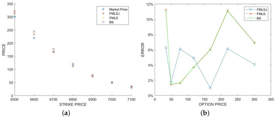
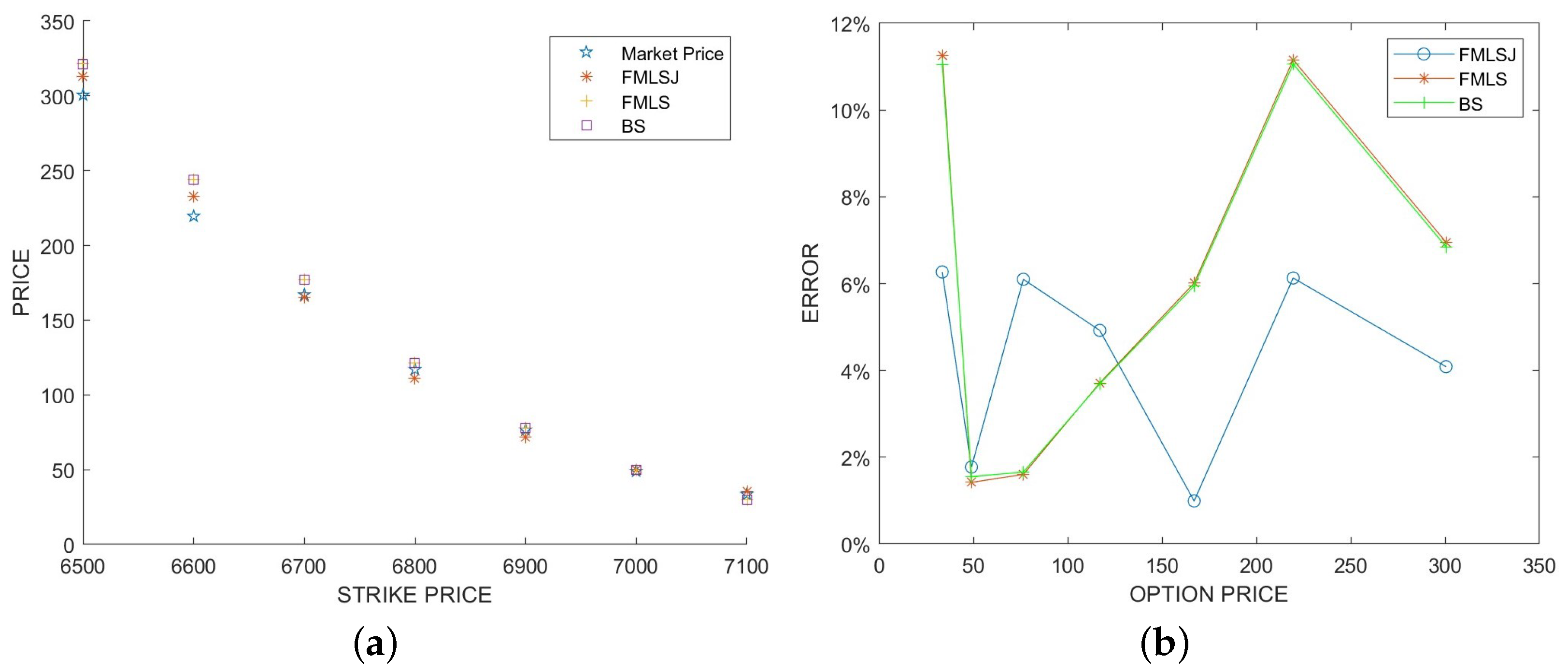
Figure 1. Comparisons between three models. (a) Option price comparison. (b) Pricing errors of three models.

Figure 1a offers a comparison of the three models against the actual option prices. From the figure, it can be observed that the prices calculated via the FMLS model and the BS model are relatively similar, which explains why their MSEs are close to each other. In contrast, the FMLSJ model’s prices are closer to the actual prices. Figure 1b presents the relative errors under different option prices. This figure also demonstrates that the errors of the FMLS model and the BS model are very similar. Meanwhile, the relative errors of the FMLSJ model are all below $7\%$, indicating superior performance compared to the first two models.

In the second numerical test of this example, the parameters listed in Table 1, obtained from the option contract SR403, are used to assess the performance of the proposed fast solution strategy. The other parameters are set as follows: $r=2.561\%$, $T=1$, $x_{max}=ln\left(100\right)$, $x_{min}=ln\left(0.1\right)$, $K=50$. Additionally, to evaluate the effectiveness of the banded preconditioner used in this paper, the preconditioner based on the circulant approximation from [38] is employed for comparison. Specifically, this preconditioner is defined as:

$$P_s=\Phi [(1-\tau c_3)I_N+\frac{\tau c_1}{h}D+\frac{\tau c_2}{h^{\alpha }}s\left(G\right)+\tau c_{4}s\left(S\right)]+(1-\Phi )I_N,$$

(21)

where $s(.)$ denotes Strang’s approximation.

For simplicity, the following text will use the notation GMRES to refer to the GMRES algorithm without preconditioning, SGMRES to denote the GMRES algorithm with the circulant preconditioner (21), and BGMRES(l) to indicate the GMRES method preconditioned by the banded preconditioner with $2l-1$ bands. Additionally, in the following tables, “Error” represents the infinite norm of the error between the numerical solution and the exact solution, “Rate” represents the convergence rate, “Iter-Out” indicates the average number of iterations of the policy iteration method on each time level, and “Iter-In” refers to the average number of iterations of the Krylov subspace method on each policy iteration. Note that the numerical solution on a fine grid with $\tilde{N}=2^{16}$ and $M=2^{12}$ is regarded as the exact solution since its analytical solution is unknown.

From Table 2, it is evident that since the outer iterations all employ the policy iteration method, the number of outer iterations remains the same, as do the errors and convergence order. Meanwhile, Table 3 demonstrates that compared to circulant preconditioning, the band preconditioning method performs better. Additionally, when comparing different values of l, BGMRES(4) achieves good results with the lowest CPU time, whereas $l=7$ and $l=13$ do not improve the number of iterations in this example and lead to higher CPU times due to the increased computational effort required for obtaining its inversion. Therefore, $l=4$ is found to be sufficient to achieve good results, both in terms of the number of iterations and CPU time.

Table 2. Comparisons of errors and outer iteration numbers.

		GMRES			SGMRES			BGMRES (4)
$\tilde{\mathit{N}}$	$\mathit{M}$	Error	Rate	Iter-Out	Error	Rate	Iter-Out	Error	Rate	Iter-Out
$2^{10}$	$2^5$	$1.1432\times {10}^{-2}$	-	2.0	$1.1432\times {10}^{-2}$	-	2.0	$1.1432\times {10}^{-2}$	-	2.0
$2^{11}$	$2^6$	$5.6617\times {10}^{-3}$	1.0138	2.0	$5.6617\times {10}^{-3}$	1.0138	2.0	$5.6617\times {10}^{-3}$	1.0138	2.0
$2^{12}$	$2^7$	$2.6366\times {10}^{-3}$	1.1026	2.0	$2.6366\times {10}^{-3}$	1.1026	2.0	$2.6366\times {10}^{-3}$	1.1026	2.0
$2^{13}$	$2^8$	$1.2406\times {10}^{-3}$	1.0876	2.0	$1.2406\times {10}^{-3}$	1.0876	2.0	$1.2406\times {10}^{-3}$	1.0876	2.0
$2^{14}$	$2^9$	$5.3396\times {10}^{-4}$	1.2163	2.0	$5.3396\times {10}^{-4}$	1.2163	2.0	$5.3396\times {10}^{-4}$	1.2163	2.0

Table 3. Comparisons between different linear solvers.

Method	$\tilde{\mathit{N}}=2^{11}$	$\mathit{M}=2^6$	$\tilde{\mathit{N}}=2^{12}$	$\mathit{M}=2^7$	$\tilde{\mathit{N}}=2^{13}$	$\mathit{M}=2^8$	$\tilde{\mathit{N}}=2^{14}$	$\mathit{M}=2^9$
	Iter-In	Time (s)	Iter-In	Time (s)	Iter-In	Time (s)	Iter-In	Time (s)
GMRES	49.0	1.89	70.0	6.67	100.0	70.15	146.0	416.42
SGMRES	18.6	1.35	30.4	4.05	45.8	51.31	68.0	316.21
BGMRES(2)	4.0	0.32	4.0	0.58	4.0	4.12	4.0	17.29
BGMRES(4)	4.0	0.28	3.0	0.52	3.0	3.61	3.0	15.22
BGMRES(7)	4.0	0.30	3.0	0.64	3.0	4.18	3.0	18.10
BGMRES(13)	4.0	0.37	3.0	0.87	3.0	5.92	3.0	23.64

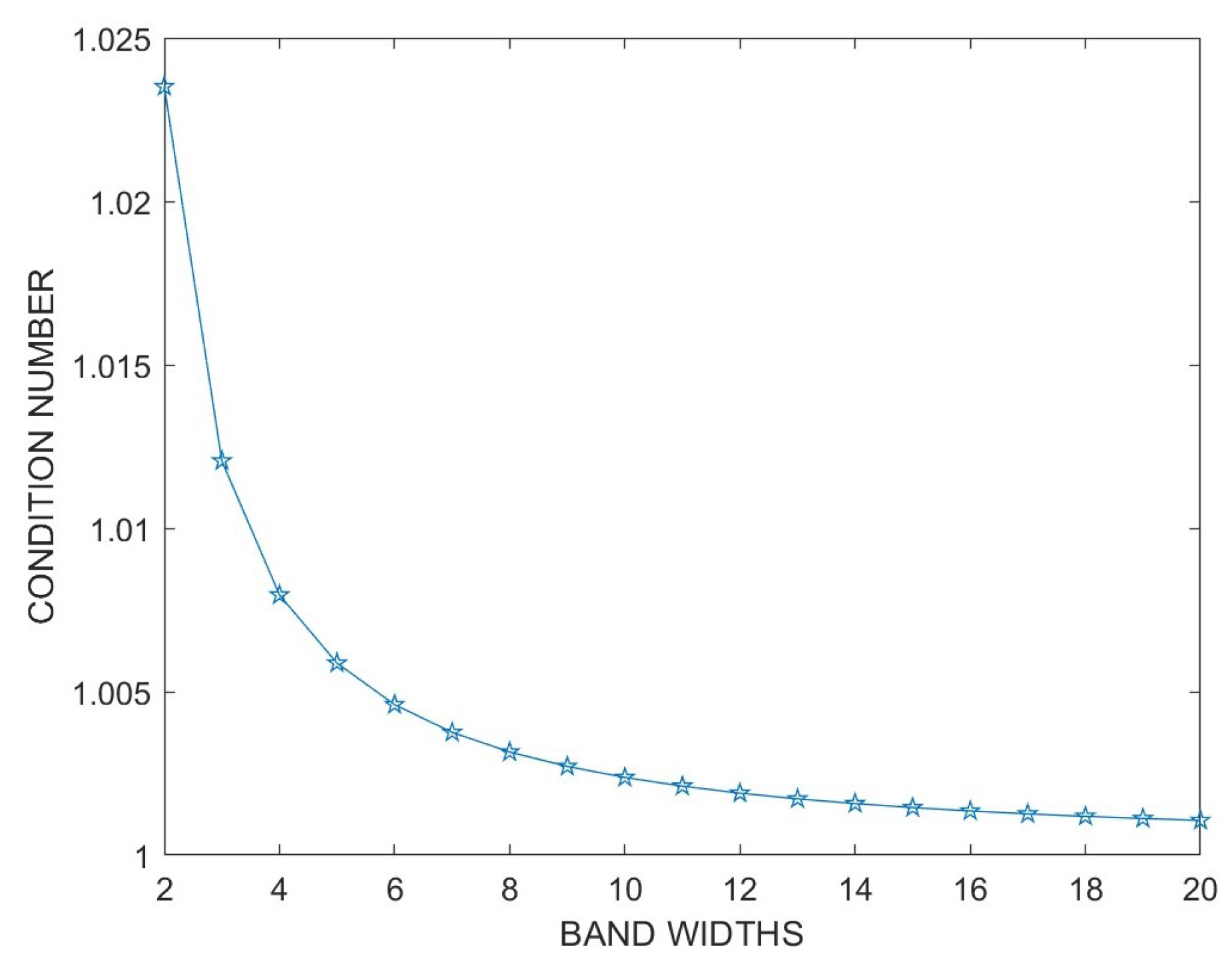
Additionally, to verify the effectiveness of Theorem 4, the condition numbers of the preconditioning matrices for different l will be presented. However, it should be noted that the coefficient matrix in the policy iteration method changes with each time step and iteration. To facilitate verification, the parameters of the model from Table 2 are utilized, with $\tilde{N}=2^{14}$, $M=2^7$, and $\Phi =\mathrm{diag}({\varphi }_1,{\varphi }_2,\dots ,{\varphi }_N)$, where

$${\varphi }_i=\left\{\begin{array}{c}0,\mathrm{for}i\le \lfloor \frac{\tilde{N}-1}{2}\rfloor ,\hfill \\ 1,\mathrm{for}i>\lfloor \frac{\tilde{N}-1}{2}\rfloor .\hfill \end{array}\right.$$

Then, the condition number of the coefficient matrix M is $365.1499$. The condition numbers of the preconditioned coefficient matrix for various l values are depicted in Figure 2.

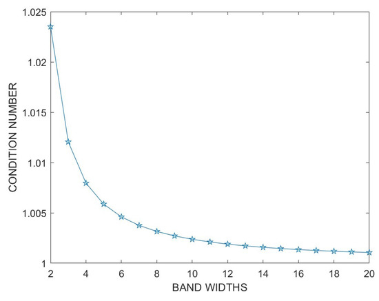
Figure 2. Condition number of the preconditioned matrix.

As stated in Theorem 4, it is observed from Figure 2 that as l increases, the condition number gradually decreases and more closely approaches 1. Given that the original condition number reaches $365.1499$, it can be seen that the banded preconditioner effectively reduces the condition number of the coefficient matrix, and when $l=2$, the condition number is already very close to 1.

6.2. Stock Loan

In this part, we consider a stock loan problem to test the performance of the proposed preconditioned policy–Krylov subspace method. The parameters are set as follows: $\sigma =0.2$, $\tilde{\lambda }=0.01$, $u_J=0.8$, ${\sigma }_J=0.01$, $\gamma =0.1$, $r=0.05$, $T=1$. Experience from Example 1 indicates that a smaller value of l can achieve satisfactory results, so in this example, the value of l is uniformly set to 4. Additionally, in this example, the value of $\alpha$ will be set to 1.2, 1.5, and 1.8, respectively, to assess the algorithm’s performance with different fractional orders. Similar to Example 1, the numerical solution on a fine grid with $\tilde{N}=2^{15}$ and $M=2^{11}$ is regarded as the exact solution.

For $\alpha =1.2$, $1.5$, and $1.8$, the comparison results of different iterative methods are presented in Table 4, Table 5 and Table 6, respectively. The errors in these tables are derived from the results of the BGMRES(4) method. It is observed that the convergence rate is first order for all results. Compared with the results of the iterative method without preconditioning, it is evident that as $\alpha$ increases, more iterations are required. However, both the circulant preconditioner and the proposed banded preconditioner can reduce the number of iterations, with the band preconditioning technique demonstrating significantly better performance in terms of both the number of iterations and CPU time.

Table 4. Algorithm comparison for $\alpha =1.2$.

	$\tilde{\mathit{N}}$	M	Error	Rate	Iter-Out	Iter-In	Time (s)
GMRES	$2^{10}$	$2^6$	$1.9624\times {10}^{-1}$	0.9531	2.0	40.9	0.62
	$2^{11}$	$2^7$	$9.7790\times {10}^{-2}$	1.0049	2.0	45.0	3.51
	$2^{12}$	$2^8$	$4.6303\times {10}^{-2}$	1.0786	2.0	49.0	9.54
	$2^{13}$	$2^9$	$2.0009\times {10}^{-2}$	1.2104	2.0	54.0	69.94
SGMRES	$2^{10}$	$2^6$	$1.9624\times {10}^{-1}$	0.9531	2.0	13.8	0.29
	$2^{11}$	$2^7$	$9.7790\times {10}^{-2}$	1.0049	2.0	14.6	1.88
	$2^{12}$	$2^8$	$4.6303\times {10}^{-2}$	1.0786	2.0	16.2	3.93
	$2^{13}$	$2^9$	$2.0009\times {10}^{-2}$	1.2104	2.0	17.6	39.81
BGMRES (4)	$2^{10}$	$2^6$	$1.9624\times {10}^{-1}$	0.9531	2.0	7.0	0.15
	$2^{11}$	$2^7$	$9.7790\times {10}^{-2}$	1.0049	2.0	7.0	0.74
	$2^{12}$	$2^8$	$4.6303\times {10}^{-2}$	1.0786	2.0	7.0	1.68
	$2^{13}$	$2^9$	$2.0009\times {10}^{-2}$	1.2104	2.0	7.0	11.83

Table 5. Algorithm comparison for $\alpha =1.5$.

	$\tilde{\mathit{N}}$	M	Error	Rate	Iter-Out	Iter-In	Time (s)
GMRES	$2^{10}$	$2^6$	$4.0928\times {10}^{-2}$	1.0024	2.0	44.9	0.67
	$2^{11}$	$2^7$	$2.0015\times {10}^{-2}$	1.0320	2.0	55.0	4.25
	$2^{12}$	$2^8$	$9.3484\times {10}^{-3}$	1.0983	2.0	68.0	13.29
	$2^{13}$	$2^9$	$4.0197\times {10}^{-3}$	1.2176	2.0	84.0	119.81
SGMRES	$2^{10}$	$2^6$	$4.0928\times {10}^{-2}$	1.0024	2.0	14.7	0.32
	$2^{11}$	$2^7$	$2.0015\times {10}^{-2}$	1.0320	2.0	17.8	2.27
	$2^{12}$	$2^8$	$9.3484\times {10}^{-3}$	1.0983	2.0	22.0	5.90
	$2^{13}$	$2^9$	$4.0197\times {10}^{-3}$	1.2176	2.0	27.4	65.05
BGMRES (4)	$2^{10}$	$2^6$	$4.0928\times {10}^{-2}$	1.0024	2.0	7.2	0.16
	$2^{11}$	$2^7$	$2.0015\times {10}^{-2}$	1.0320	2.0	8.0	0.85
	$2^{12}$	$2^8$	$9.3484\times {10}^{-3}$	1.0983	2.0	8.0	1.95
	$2^{13}$	$2^9$	$4.0197\times {10}^{-3}$	1.2176	2.0	8.7	15.35

Table 6. Algorithm comparison for $\alpha =1.8$.

	$\tilde{\mathit{N}}$	M	Error	Rate	Iter-Out	Iter-In	Time (s)
GMRES	$2^{10}$	$2^6$	$1.2786\times {10}^{-2}$	1.0394	2.3	53.0	0.88
	$2^{11}$	$2^7$	$6.1931\times {10}^{-3}$	1.0459	2.2	68.8	5.98
	$2^{12}$	$2^8$	$3.1333\times {10}^{-3}$	0.9830	2.2	89.5	19.49
	$2^{13}$	$2^9$	$1.4819\times {10}^{-3}$	1.0802	2.2	117.8	165.29
SGMRES	$2^{10}$	$2^6$	$1.2786\times {10}^{-2}$	1.0394	2.3	21.2	0.64
	$2^{11}$	$2^7$	$6.1931\times {10}^{-3}$	1.0459	2.2	29.6	4.08
	$2^{12}$	$2^8$	$3.1333\times {10}^{-3}$	0.9830	2.2	39.2	11.21
	$2^{13}$	$2^9$	$1.4819\times {10}^{-3}$	1.0802	2.2	52.9	125.92
BGMRES (4)	$2^{10}$	$2^6$	$1.2786\times {10}^{-2}$	1.0394	2.3	7.0	0.18
	$2^{11}$	$2^7$	$6.1931\times {10}^{-3}$	1.0459	2.2	8.0	0.94
	$2^{12}$	$2^8$	$3.1333\times {10}^{-3}$	0.9830	2.2	8.0	2.10
	$2^{13}$	$2^9$	$1.4819\times {10}^{-3}$	1.0802	2.2	9.0	15.82

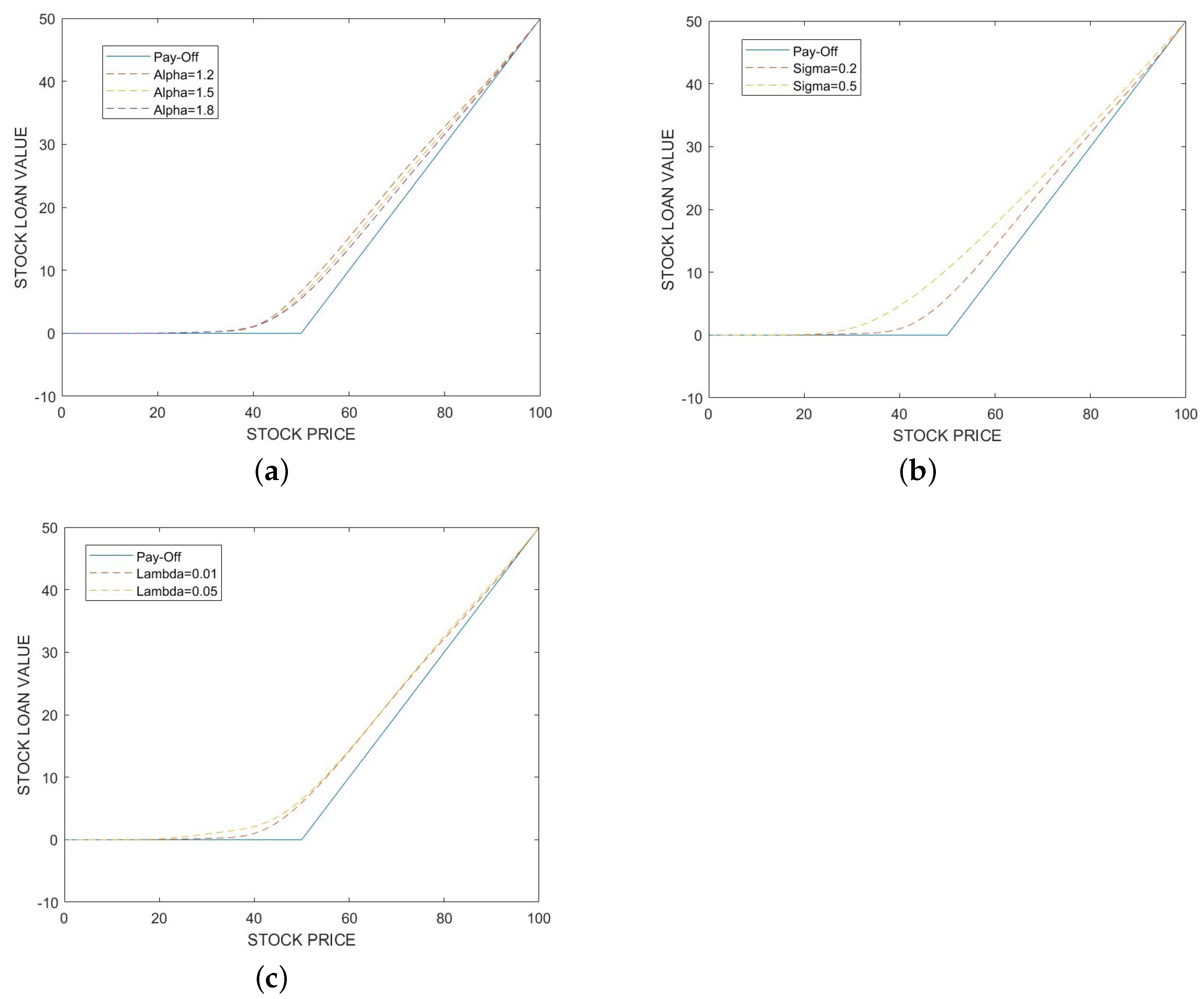
To further illustrate the effectiveness of the model and the impact of its parameters, Figure 3 is presented. The same parameters from this subsection are used, specified as follows: $u_J=0.8$, ${\sigma }_J=0.01$, $\gamma =0.1$, $r=0.05$, $T=1$. Any missing parameters are provided in the figure captions. Additionally, all models are solved using the BGMRES(4) method with settings of $\tilde{N}=2^{12}$ and $M=2^{10}$. The figures demonstrate that the stock loan prices, similar to American call options, are positioned above the pay-off function. Figure 3a shows that as $\alpha$ increases, the curve approaches the pay-off function, aligning with results from Ref. [42]. Figure 3b illustrates that as volatility $\sigma$ increases, the price of the stock loan becomes higher. Figure 3c indicates that as $\tilde{\lambda }$, the jump frequency, increases, price fluctuations become more frequent, thereby enhancing the value of the stock loan. These figures confirm that the solutions obtained from the considered model meet our expectations for the curve of stock loan valuation.

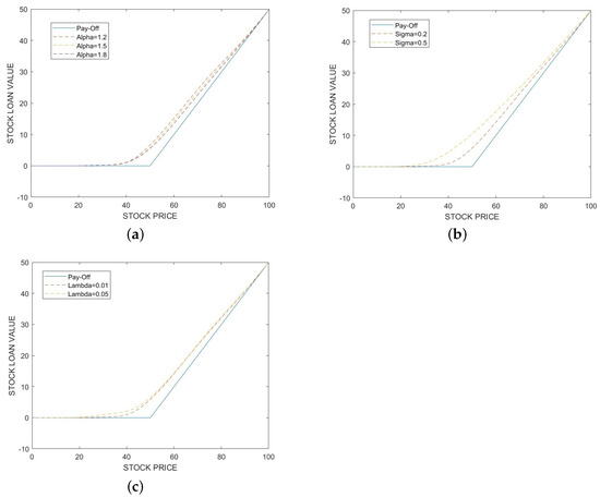
Figure 3. Comparative analysis of stock loan values. (a) Comparison of different $\alpha$ with $\sigma =0.2$ and $\tilde{\lambda }=0.01$. (b) Comparison of different $\sigma$ with $\alpha =1.5$ and $\tilde{\lambda }=0.01$. (c) Comparison of different $\tilde{\lambda }$ with $\sigma =0.2$ and $\alpha =1.5$.

7. Conclusions

In this paper, we consider a fractional partial integro-differential HJB equation resulting from the American option pricing and stock loan pricing based on the Lévy-$\alpha$-stable process with jumps model, and propose a preconditioned policy–Krylov subspace method to solve it. A finite difference scheme is developed to discretize the HJB equation, with stability and first-order convergence analysis. The coefficient matrix generated from the fractional derivative and the integro-differential operator is an $\mathcal{M}$-matrix and possesses the Toeplitz structure, leading us to use the policy iteration method and the fast Krylov subspace method as the outer and inner iterative methods, respectively. To accelerate the convergence rate of the Krylov subspace method, a banded preconditioner is proposed. It is proven that the condition number of the preconditioned matrix has an upper boundary affected by the bandwidth. Finally, numerical examples of an American options pricing problem and a stock loan valuation problem are provided to demonstrate the effectiveness of the proposed fast solution strategy.

References

- Black, F.; Scholes, M. The pricing of options and corporate liabilities. J. Polit. Econ. 1973, 81, 637–654. [Google Scholar] [CrossRef]
- Heston, S.L. A closed-form solution for options with stochastic volatility with applications to bond and currency options. Rev. Financ. Stud. 1993, 6, 327–343. [Google Scholar] [CrossRef]
- Stein, E.M.; Stein, J.C. Stock price distributions with stochastic volatility: An analytic approach. Rev. Financ. Stud. 1991, 4, 727–752. [Google Scholar] [CrossRef]
- Kou, S.G. A jump-diffusion model for option pricing. Manage. Sci. 2002, 48, 1086–1101. [Google Scholar] [CrossRef]
- Fulop, A.; Li, J.; Yu, J. Self-exciting jumps, learning, and asset pricing implications. Rev. Financ. Stud. 2015, 28, 876–912. [Google Scholar] [CrossRef]
- Hawkes, A.G. Hawkes jump-diffusions and finance: A brief history and review. Eur. J. Financ. 2022, 28, 627–641. [Google Scholar] [CrossRef]
- Wang, Y.; Wang, J. Pricing of American Carbon Emission Derivatives and Numerical Method under the Mixed Fractional Brownian Motion. Discrete Dyn. Nat. Soc. 2021, 2021, 6612284. [Google Scholar] [CrossRef]
- Huang, S.; He, X. Analytical approximation of European option prices under a new two-factor non-affine stochastic volatility model. AIMS. Math. 2022, 8, 4875–4891. [Google Scholar] [CrossRef]
- Bian, L.; Li, Z. Fuzzy simulation of European option pricing using sub-fractional Brownian motion. Chaos Solitons Fractals 2021, 153, 111442. [Google Scholar] [CrossRef]
- Guo, Z.; Liu, Y.; Dai, L. European option pricing under sub-fractional Brownian motion regime in discrete time. Fractal Fract. 2024, 8, 13. [Google Scholar] [CrossRef]
- Cartea, A.; del Castillo-Negrete, D. Fractional diffusion models of option prices in markets with jumps. Phys. A 2007, 374, 749–763. [Google Scholar] [CrossRef]
- Boyarchenko, S.; Levendorskii, S. Non-Gaussian Merton-Black–Scholes Theory; World Scientific: Singapore, 2002. [Google Scholar]
- Carr, P.; Geman, H.; Madan, D.B.; Yor, M. The fine structure of asset returns: An empirical investigation. J. Bus. 2002, 75, 305–333. [Google Scholar] [CrossRef]
- Carr, P.; Wu, L. The finite moment log stable process and option pricing. J. Financ. 2003, 58, 753–777. [Google Scholar] [CrossRef]
- Zhou, Z.; Ma, J.; Gao, X. Convergence of iterative laplace transform methods for a system of fractional PDEs amd PIDEs arising in option pricing. East Asian Appl. Math. 2018, 8, 782–808. [Google Scholar] [CrossRef]
- Fan, C.; Chen, W.; Feng, B. Pricing stock loans under the Lévy-α-stable process with jumps. Netw. Heterog. Media 2023, 18, 191–211. [Google Scholar] [CrossRef]
- Boyarchenko, S.; Levendorskii, S. American options in regime-switching models. SIAM J. Control Optim. 2009, 48, 1353–1376. [Google Scholar] [CrossRef]
- Yousuf, M.; Khaliq, A.; Liu, R. Pricing American options under multi-state regime switching with an efficient L-stable method. Int. J. Comput. Math. 2015, 92, 2530–2550. [Google Scholar] [CrossRef]
- Khaliq, A.; Voss, D.; Kazmi, S. A linearly implicit predictor–corrector scheme for pricing American options using a penalty method approach. J. Bank Financ. 2006, 30, 489–502. [Google Scholar] [CrossRef]
- Wang, W.; Chen, Y.; Fang, H. On the variable two-step IMEX BDF method for parabolic integro-differential equations with nonsmooth initial data arising in finance. SIAM J. Numer. Anal. 2019, 57, 1289–1317. [Google Scholar] [CrossRef]
- Shi, X.; Yang, L.; Huang, Z. A fixed point method for the linear complementarity problem arising from American option pricing. Acta Math. Appl. Sin. Engl. Ser. 2016, 32, 921–932. [Google Scholar] [CrossRef]
- Lei, S.; Wang, W.; Chen, X.; Ding, D. A fast preconditioned penalty method for American options pricing under regime-switching tempered fractional diffusion models. J. Sci. Comput. 2018, 75, 1633–1655. [Google Scholar] [CrossRef]
- Bai, Z. Modulus-based matrix splitting iteration methods for linear complementarity problems. Numer. Linear Algebra Appl. 2010, 17, 917–933. [Google Scholar] [CrossRef]
- Saigal, R. On the Convergence Rate of Algorithms for Solving Equations That Are Based on Methods of Complementary Pivoting. Math. Oper. Res. 1977, 2, 108–124. [Google Scholar] [CrossRef]
- Toivanen, J.; Oosterlee, C.W. A projected algebraic multigrid method for linear complementarity problems. Numer. Math. Theor. Meth. Appl. 2012, 5, 85–98. [Google Scholar] [CrossRef]
- Chen, Y.; Wan, J.W.L. Deep neural network framework based on backward stochastic differential equations for pricing and hedging American options in high dimensions. Quant. Financ. 2021, 21, 45–67. [Google Scholar] [CrossRef]
- Gatta, F.; Cola, V.S.D.; Giampaolo, F.; Piccialli, F.; Cuomo, S. Meshless methods for American option pricing through Physics-Informed Neural Networks. Eng. Anal. Boundary Elem. 2023, 151, 68–82. [Google Scholar] [CrossRef]
- Reisinger, C.; Witte, J.H. On the use of policy iteration as an easy way of pricing American options. SIAM J. Financ. Math. 2012, 3, 459–478. [Google Scholar] [CrossRef]
- Podlubny, I. Fractional Differential Equations; Academic Press: New York, NY, USA, 1999. [Google Scholar]
- Pascucci, A.; Suarez-Taboada, M.; Vazquez, C. Mathematical analysis and numerical methods for a PDE model of a stock loan pricing problem. J. Math. Anal. Appl. 2013, 403, 38–53. [Google Scholar] [CrossRef]
- Pang, H.; Zhang, Y.; Vong, S.; Jin, X. Circulant preconditioners for pricing options. Linear Algebra Appl. 2011, 434, 2325–2342. [Google Scholar] [CrossRef]
- Lesmana, D.C.; Wang, S. An upwind finite difference method for a nonlinear Black–Scholes equation governing European option valuation under transaction costs. Appl. Math. Comput. 2013, 219, 8811–8828. [Google Scholar] [CrossRef]
- Zhou, Z.; Ma, J.; Sun, H. Fast Laplace transform methods for free-boundary problems of fractional diffusion equations. J. Sci. Comput. 2018, 74, 49–69. [Google Scholar] [CrossRef]
- Meerschaert, M.M.; Tadjeran, C. Finite difference approximations for fractional advection–dispersion flow equations. Comput. Appl. Math. 2004, 172, 65–77. [Google Scholar] [CrossRef]
- Plemmons, R.J. M-matrix characterizations. I—nonsingular M-matrices. Linear Algebra Appl. 1977, 18, 175–188. [Google Scholar] [CrossRef]
- Huang, Y.; Forsyth, P.A.; Labahn, G. Methods for pricing American options under regime switching. SIAM J. Sci. Comput. 2011, 33, 2144–2168. [Google Scholar] [CrossRef]
- Varah, J.M. A lower bound for the smallest singular value of a matrix. Linear Algebra Appl. 1975, 11, 3–5. [Google Scholar] [CrossRef]
- Chen, X.; Wang, W.; Ding, D.; Lei, S. A fast preconditioned policy iteration method for solving the tempered fractional HJB equation governing American options valuation. Comput. Appl. Math. 2017, 73, 1932–1944. [Google Scholar] [CrossRef]
- Wang, Q.; She, Z.; Lao, C.; Lin, F. Fractional centered difference schemes and banded preconditioners for nonlinear Riesz space variable-order fractional diffusion equations. Numer. Algorithms 2024, 95, 859–895. [Google Scholar] [CrossRef]
- She, Z.; Lao, C.; Yang, H.; Lin, F. Banded Preconditioners for Riesz Space Fractional Diffusion Equations. J. Sci. Comput. 2021, 86, 31. [Google Scholar] [CrossRef]
- Saad, Y.; Schultz, M. GMRES: A generalized minimal residual algorithm for solving nonsymmetric linear systems. SIAM J. Sci. Statist. Comput. 1986, 7, 856–869. [Google Scholar] [CrossRef]
- Aguilar, J.; Korbel, J. Simple formulas for pricing and hedging European options in the finite moment log-stable model. Risks 2019, 7, 36. [Google Scholar] [CrossRef]
Disclaimer/Publisher’s Note: The statements, opinions and data contained in all publications are solely those of the individual author(s) and contributor(s) and not of MDPI and/or the editor(s). MDPI and/or the editor(s) disclaim responsibility for any injury to people or property resulting from any ideas, methods, instructions or products referred to in the content. |
© 2024 by the authors. Licensee MDPI, Basel, Switzerland. This article is an open access article distributed under the terms and conditions of the Creative Commons Attribution (CC BY) license (https://creativecommons.org/licenses/by/4.0/).