Exploring the Depths: Soliton Solutions, Chaotic Analysis, and Sensitivity Analysis in Nonlinear Optical Fibers

Abstract

This paper discusses the time-fractional nonlinear Schrödinger model with optical soliton solutions. We employ the $\left(f+\left(\frac{G^{\prime }}{G}\right)\right)$-expansion method to attain the optical solution solutions. An important tool for explaining the particular explosion of brief pulses in optical fibers is the nonlinear Schrödinger model. It can also be utilized in a telecommunications system. The suggested method yields trigonometric solutions such as dark, bright, kink, and anti-kink-type optical soliton solutions. Mathematica 11 software creates 2D and 3D graphs for many physically important parameters. The computational method is effective and generally appropriate for solving analytical problems related to complicated nonlinear issues that have emerged in the recent history of nonlinear optics and mathematical physics. Furthermore, we venture into uncharted territory by subjecting our model to chaotic and sensitivity analysis, shedding light on its robustness and responsiveness to perturbations. The proposed technique is being applied to this model for the first time.

1. Introduction

Solitons function similarly to Fourier modes in linear media and are now recognized as essential building blocks of modes in nonlinear dispersive media. Specifically, the particle (fermion) idea in the inverse scattering transform (IST) is supported by identifying a soliton as an eigenvalue. Concurrently, it was shown that self-focusing was possible in a Kerr medium [1], and it was shown that the balance between refraction and cubic nonlinearity led to the emergence of a spatially localized solution resembling a soliton. Due to its increasing importance, scientific research has concentrated heavily on studying nonlinear partial differential equations (PDEs). Various scientific domains use nonlinear PDEs, such as the earth sciences, physics, mathematics, engineering, and other technological sectors. Research has concentrated on understanding and solving these nonlinear PDEs for a long time, both analytically and numerically. For nonlinear PDEs and nonlinear optics in physics-related fields, including fluid mechanics, plasma theory, and nonlinear optics, numerous solitary wave solutions have been found in the domain of precise solutions. NLS equations have become vital instruments for discussing various physical events in many scientific domains.

Nonlinear partial differential equations (NPDEs) govern most physical phenomena and dynamical systems. The study of nonlinear wave propagation issues has promoted the development of NPDEs. The primary goal in nonlinear physics is to find solutions to NPDEs, predominantly solitary and soliton wave solutions. Solutions aid in the understanding of nonlinear physical and natural systems. In several basic sciences, including mathematics and engineering, non-partial differential equations (NPDEs) are used to approximate a variety of processes and dynamics [2,3,4,5,6].

Russell developed the key concept of the soliton in 1844 [7], based on a coincidental thought that happened on the Edinburgh–Glasgow Canal in 1834, referred to as “a great translation wave”. This phenomenon was eventually named “solitary waves” because of the shape of the single pulse. Therefore, two of the well-known researchers who have conducted a hypothetical examination on lone waves are Boussinesc and Rayleigh [7]. Since then, single-wave research has developed to become one of the main fields of study for single waves. Solitary waves that are self-contained, strong, steady, and persistent do not disperse and hold onto their identity as they move across the medium. They include high-speed media transmissions and the occurrence of controlled solitons in numerous crucial fields of physics and technology. Solitons are self-positioning wave units with their own Broglie wavelength equivalents due to Galilean symmetry. Conversely, the soliton, an extended particle-like object, has negative self-interaction energy (binding energy) and is bound by nonlinear self-interaction at the self-induced trapping potential. It provides details on the geometry and form of solitons [8].

Many researchers utilized diverse algorithms to find the analytical solution such as the Sine–Gordon expansion algorithm [9,10], the Jacobi-elliptic technique [11], the homogeneous balance technique [12], the modified simple equation approach [13,14,15], the auxiliary equation technique [16,17], the modified extended direct algebraic method [18], the extended tanh expansion method [19], $\left(\frac{G^{\prime }}{G}\right)$-expansion technique [20], the Auto-Bäcklund transformation [21], and Hirota’s bilinear technique [22]. A variety of fractional derivatives are essential to the physical phenomena of nonlinear partial differential equations, such as the Beta derivative [20], Jumarie’s modified Riemann–Liouville derivative [23], the Riemann–Liouville derivative [24], the fractal derivatives [25], Atangana’s conformable derivative [26], the Caputo derivative [27], and the Atangana–Baleanu fractional operator [28]. The coupled NLSE is utilized to search out the wave propagation in continuous mediums [29], which happens in the typical scenario arising slowly fluctuating waves of small amplitude, like the long-distance pulse propagation in fluid dynamics, optical fibers, nonlinear optics, quantum mechanics, and other physical nature [30,31], which reads

$$D_x{D}_t^{\beta }v=D_{xx}v+\frac{2}{1-{\delta }^2}\mid v^2\mid v+v(r-u),$$

(1)

$$D_t^{\beta }r=-\frac{D_t^{\beta }(\mid v{\mid }^2)}{1+\delta }+(1+\delta )D_{x}r,$$

(2)

$$D_t^{\beta }u=\frac{D_t^{\beta }(\mid v{\mid }^2)}{1+\delta }+(1-\delta )D_{x}u,$$

(3)

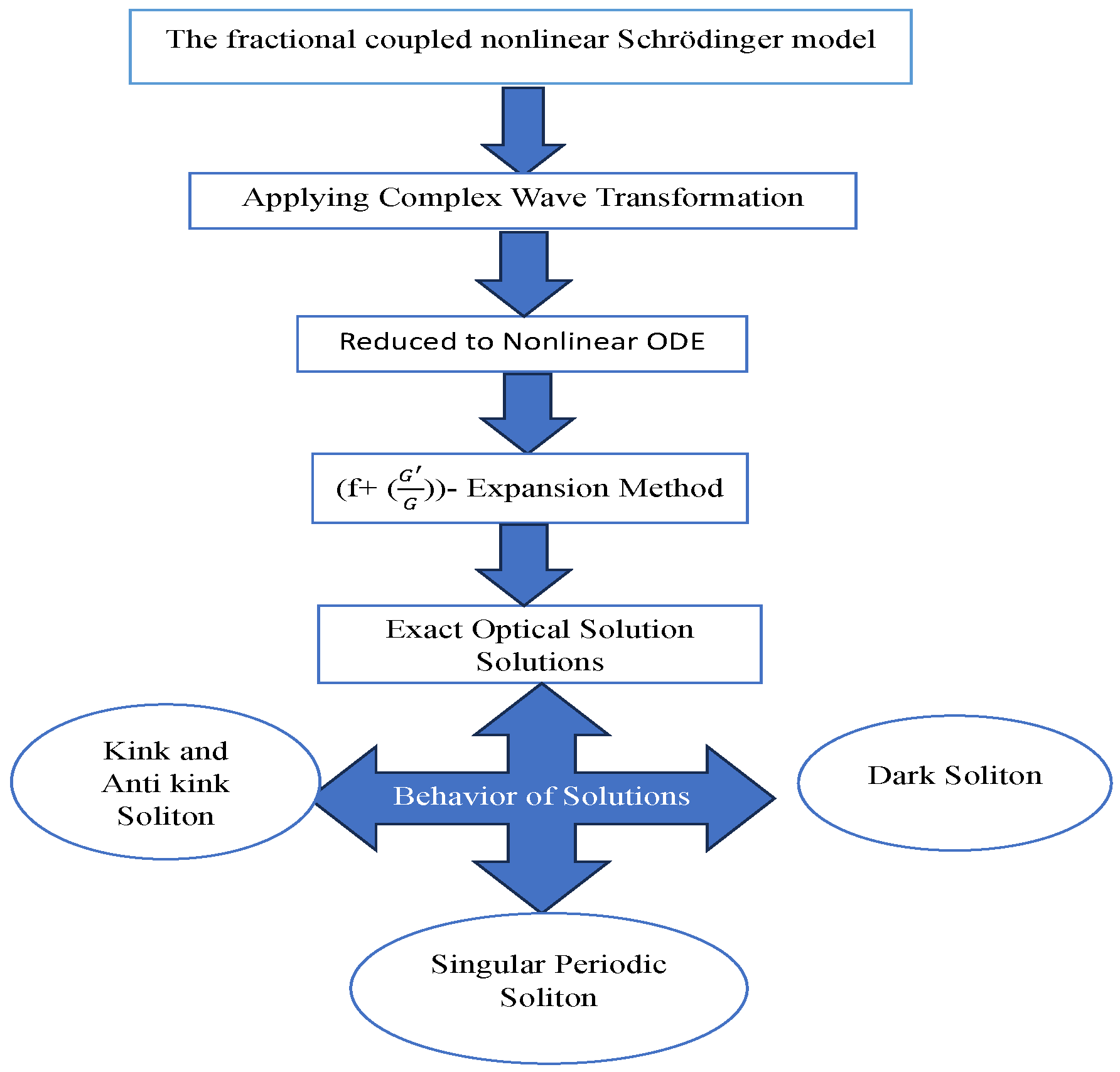
where $r(x,t)$ and $u(x,t)$ are the real functions, $v(x,t)$ is a complex function of time t and x. The parameters $\beta$ are the fractional order of derivatives having values $\beta \ge 0$. Moreover Equations (1)–(3) describe non-relativistic quantum mechanical behavior and nonlinear media. The main idea of this study is shown in Figure 1. The present study is distributed into different sections. In Section 2, we present the beta derivative and the description of the algorithm. Section 3 presents the optical solitary wave solution of the considered model. Section 4 presents the chaotic analysis and Section 5 presents the sensitivity analysis. The results attained through $\left(f+\left(\frac{G^{\prime }}{G}\right)\right)$-expansion algorithm will be analyzed graphically in Section 6. The conclusion is presented in Section 7.

Figure 1. Flow Chart Diagram.

2. Beta Derivative

Definition 1. 

Let $g\left(t\right)$ be a function defined for all non-negative ts. Then, the beta derivative of $g\left(t\right)$ of order β is given by [20]

$$T^{\beta }g\left(t\right)=\frac{d^{\beta }g\left(t\right)}{d{t}^{\beta }}=\underset{ϵ\to 0}{lim}\frac{g(t+ϵ{(t+\frac{1}{\Gamma \left(\beta \right)})}^{1-\beta })-g\left(t\right)}{ϵ},$$

where $0<\beta \le 1$.

Algorithm of the $\left(f+\left(\frac{G^{\prime }}{G}\right)\right)$-Expansion Method

Consider the NPDE as

$$P(v,v_x,v_y,v_z,v_t,v_{tt},v_{xx},v_{xt},...)=0.$$

(4)

In which P is a polynomial in v and its derivatives. The main steps are given as follows:

Step 1: Assume a wave transformation,

$$v(x,t)=V\left(\varphi \right),\varphi =x-ct.$$

(5)

Equation (5) is used in (4), then ODE is as follows:

$$H(V,V^{\prime },V^{″},V^{‴},...)=0,$$

(6)

where H is a function of $V\left(\varphi \right)$, and the prime represents its derivatives with respect to $\varphi$.

Step 2: The general form of (6) is defined as follows:

$$V\left(\varphi \right)=\sum _{i=-m}^M{\alpha }_i{(\Phi \left(\varphi \right))}^i,$$

(7)

where

$$\Phi \left(\varphi \right)=[f+\frac{G^{\prime }\left(\varphi \right)}{G\left(\varphi \right)}].$$

(8)

Here, f is constant, and its value can be found later; the values of ${\alpha }_{-m}$, or ${\alpha }_m$, may be zero, but all of them could not be zero at a time. The second order NODE satisfies for $G=G\left(\varphi \right)$, as follows:

$$G{G}^{″}=\omega G{G}^{\prime }+\xi G^2+\psi {\left(G^{\prime }\right)}^2.$$

(9)

Here, $\psi ,\xi$, and $\omega$ are real variables, and prime denotes the derivative of $\varphi$.

Equation (8) can be converted into the Riccati equation by utilizing the Col-Hopf transformation $\Psi \left(\varphi \right)={\left(\ln \left(G\right(\varphi )\right)}_{\varphi }=\frac{G^{\prime }\left(\varphi \right)}{G\left(\varphi \right)}$:

$${\Psi }^{\prime }\left(\varphi \right)=\xi +\omega \Psi \left(\varphi \right)+(\psi -1){\Psi }^2\left(\varphi \right).$$

(10)

There are twenty-five single solutions for Equation (10) [20].

Step 3: Put (7)–(9) in (6), then we will obtain polynomials in $[f+\frac{G^{\prime }(\varphi }{G\left(\varphi \right)}]$ and ${[f+\frac{G^{\prime }\left(\varphi \right)}{G\left(\varphi \right)}]}^{-1}$, $(m=0,1,2,\cdots ,M)$. Substituting each coefficient of polynomials equal to zero, we obtain a set of algebraic equations.

Step 4: We can solve all algebraic equations with MATHEMATICA 11 is used to obtain the constant values. In the end, the exact wave solutions of (4) can be attained by utilizing the values of the constant together with the solutions of (9).

3. Optical Wave Solution to the Fractional NLSE

In this section, we change the fractional NLS equation into nonlinear ODEs with the help of the fractional complex transform, as follows:

$$v(x,t)=V\left(\varphi \right)e^{i\chi },r(x,t)=R\left(\varphi \right),u(x,t)=U\left(\varphi \right).$$

(11)

$$\varphi =\gamma x+\frac{\sigma }{\beta }{\left(t+\frac{1}{\Gamma \left(\beta \right)}\right)}^{\beta },\chi =\kappa x+\frac{\tau }{\beta }{\left(t+\frac{1}{\Gamma \left(\beta \right)}\right)}^{\beta },$$

(12)

where $\gamma ,\sigma ,\tau$, and $\kappa$ are the parameters. Inserting Equations (11) and (12) into (1), the real and imaginary parts are given as follows:

$$V^{″}\left(\varphi \right)+\left(\frac{\kappa (\kappa -\tau )}{\gamma (\sigma -\gamma )}\right)V\left(\varphi \right)-\left(\frac{2}{\gamma (\sigma -\gamma )(1-{\delta }^2)}\right)V^3\left(\varphi \right)+\left(\frac{u-r}{\gamma (\sigma -\gamma )}\right)V\left(\varphi \right)=0,$$

(13)

and

$$\tau \gamma +\sigma \kappa +2\gamma \kappa =0,$$

(14)

we can simplify (14),

$$\tau \gamma +\sigma \kappa +\gamma \kappa +\gamma \kappa =0.$$

$$(\tau +\kappa )\gamma +(\sigma +\gamma )\kappa =0.$$

$$(\tau +\kappa )\gamma =-(\sigma +\gamma )\kappa .$$

$$\frac{\kappa -\tau }{\sigma -\gamma }=\frac{\kappa }{\gamma }.$$

(15)

Substituting (15) into (13), we have the nonlinear ODE, as follows:

$$V^{″}\left(\varphi \right)+\left(\frac{{\kappa }^2}{{\gamma }^2}\right)V\left(\varphi \right)-\left(\frac{2}{\gamma (\sigma -\gamma )(1-{\delta }^2)}\right)V^3\left(\varphi \right)+\left(\frac{u-r}{\gamma (\sigma -\gamma )}\right)V\left(\varphi \right)=0.$$

(16)

Substituting (11) and (12) into (2) and (3), we then ingratiate the following:

$$R=\frac{-\sigma V^2}{(1+\delta )(\sigma -(1+\delta \left)\gamma \right)}.$$

(17)

$$U=\frac{\sigma V^2}{(1-\delta )(\sigma -(1-\delta \left)\gamma \right)}.$$

(18)

Substituting (17) and (18) into (16), we obtain the following:

$$V^{″}\left(\varphi \right)+\left(\frac{{\kappa }^2}{{\gamma }^2}\right)V\left(\varphi \right)-\left(\frac{2}{{\delta }^2{\gamma }^2-{(\sigma -\gamma )}^2}\right)V^3\left(\varphi \right)=0.$$

(19)

Next, we can apply the homogeneous balancing technique on (19); then we obtain $N=1$. So, Equation (6) is as follows:

$$V\left(\varphi \right)={\alpha }_{-1}{(\Phi \left(\varphi \right))}^{-1}+{\alpha }_0+{\alpha }_1\Phi \left(\varphi \right),$$

(20)

where ${\alpha }_{-1},{\alpha }_0$, and ${\alpha }_1$ are unknown parameters to be found. Substituting (20) into (16), we obtain the following set of solutions:

Set-1

$$\begin{array}{cc}\hfill & {\alpha }_{-1}=\pm \sqrt{{\gamma }^2\left({\delta }^2-1\right)+2\gamma \sigma -{\sigma }^2}\left(f^2(\psi -1)-f\omega +\xi \right),\hfill \\ & {\alpha }_0=\frac{1}{2}\sqrt{{\gamma }^2\left({\delta }^2-1\right)+2\gamma \sigma -{\sigma }^2}(2f(\psi -1)\pm \omega ),{\alpha }_1=0,\hfill \\ & \kappa =-\gamma \sqrt{2\xi (1-\psi )+\frac{{\omega }^2}{2}}.\hfill \end{array}$$

(21)

Set-2

$$\begin{array}{cc}\hfill & {\alpha }_{-1}=0,{\alpha }_0=\frac{1}{2}\sqrt{{\gamma }^2\left({\delta }^2-1\right)+2\gamma \sigma -{\sigma }^2}(\pm 2f(\psi -1)-\omega ),\hfill \\ & {\alpha }_1=\pm \left(\sqrt{{\gamma }^2\left({\delta }^2-1\right)+2\gamma \sigma -{\sigma }^2}\right)(\psi -1),\kappa =-\gamma \sqrt{2\xi (1-\psi )+\frac{{\omega }^2}{2}}.\hfill \end{array}$$

(22)

Set-3

$$\begin{array}{cc}\hfill & {\alpha }_{-1}=0,{\alpha }_0=\pm \frac{1}{2}\sqrt{{\gamma }^2\left({\delta }^2-1\right)+2\gamma \sigma -{\sigma }^2}\sqrt{{\omega }^2-4\xi (\psi -1)},\hfill \\ & {\alpha }_1=\mp (\psi -1)\left(-\sqrt{{\gamma }^2\left({\delta }^2-1\right)+2\gamma \sigma -{\sigma }^2}\right),f=\frac{\sqrt{{\omega }^2-4\xi (\psi -1)}+\omega }{2(\psi -1)},\hfill \\ & \kappa =\gamma \sqrt{2\xi (1-\psi )+\frac{{\omega }^2}{2}}.\hfill \end{array}$$

(23)

Substituting (21) into (20), the solutions to (1)–(3) are as follows:

$$\begin{array}{cc}\hfill v_1(x,t)=& (\left(\pm \sqrt{{\gamma }^2\left({\delta }^2-1\right)+2\gamma \sigma -{\sigma }^2}\left(f^2(\psi -1)-f\omega +\xi \right)\right){(\Phi \left(\varphi \right))}^{-1}\hfill \\ & +\left(\frac{1}{2}\sqrt{{\gamma }^2\left({\delta }^2-1\right)+2\gamma \sigma -{\sigma }^2}(2f(\psi -1)\pm \omega )\right))\times e^{i\chi }.\hfill \end{array}$$

(24)

$$\begin{array}{cc}\hfill R_1(x,t)=& \frac{1}{(1+\delta )(\sigma -(1+\delta \left)\gamma \right)}[-\sigma (\left(\pm \sqrt{{\gamma }^2\left({\delta }^2-1\right)+2\gamma \sigma -{\sigma }^2}\left(f^2(\psi -1)-f\omega +\xi \right)\right)\hfill \\ & {(\Phi \left(\varphi \right))}^{-1}+\left(\frac{1}{2}\sqrt{{\gamma }^2\left({\delta }^2-1\right)+2\gamma \sigma -{\sigma }^2}(2f(\psi -1)\pm \omega )\right){)}^2].\hfill \end{array}$$

(25)

$$\begin{array}{cc}\hfill U_1(x,t)=& \frac{1}{(1-\delta )(\sigma -(1-\delta \left)\gamma \right)}\left[\sigma \right(\left(\pm \sqrt{{\gamma }^2\left({\delta }^2-1\right)+2\gamma \sigma -{\sigma }^2}\left(f^2(\psi -1)-f\omega +\xi \right)\right)\hfill \\ & {(\Phi \left(\varphi \right))}^{-1}+\left(\frac{1}{2}\sqrt{{\gamma }^2\left({\delta }^2-1\right)+2\gamma \sigma -{\sigma }^2}(2f(\psi -1)\pm \omega )\right){)}^2].\hfill \end{array}$$

(26)

Furthermore, the solutions to (1)–(3) are given below.

Family 1

When $\Sigma ={\omega }^2-4\xi \psi +4\xi >0$ and $\omega (\psi -1)\ne 0$ (or $\xi (\psi -1)\ne 0$), we have

$$\begin{array}{cc}\hfill v_{1_1}(x,t)=& (\left(\pm \sqrt{{\gamma }^2\left({\delta }^2-1\right)+2\gamma \sigma -{\sigma }^2}\left(f^2(\psi -1)-f\omega +\xi \right)\right)\hfill \\ & {(f-\frac{1}{2(\psi -1)}\times (\omega +\sqrt{\Sigma }\tanh \left(\frac{1}{2}\sqrt{\Sigma }\varphi \right)))}^{-1}\hfill \\ & +\left(\frac{1}{2}\sqrt{{\gamma }^2\left({\delta }^2-1\right)+2\gamma \sigma -{\sigma }^2}(2f(\psi -1)\pm \omega )\right))\times e^{i\chi }.\hfill \end{array}$$

(27)

$$\begin{array}{cc}\hfill R_{1_1}(x,t)=& \frac{1}{(1+\delta )(\sigma -(1+\delta \left)\gamma \right)}[-\sigma (\left(\pm \sqrt{{\gamma }^2\left({\delta }^2-1\right)+2\gamma \sigma -{\sigma }^2}\left(f^2(\psi -1)-f\omega +\xi \right)\right)\hfill \\ & {(f-\frac{1}{2(\psi -1)}\times (\omega +\sqrt{\Sigma }\tanh \left(\frac{1}{2}\sqrt{\Sigma }\varphi \right)))}^{-1}\hfill \\ & +\left(\frac{1}{2}\sqrt{{\gamma }^2\left({\delta }^2-1\right)+2\gamma \sigma -{\sigma }^2}(2f(\psi -1)\pm \omega )\right){)}^2].\hfill \end{array}$$

(28)

$$\begin{array}{cc}\hfill U_{1_1}(x,t)=& \frac{1}{(1-\delta )(\sigma -(1-\delta \left)\gamma \right)}\left[\sigma \right(\left(\pm \sqrt{{\gamma }^2\left({\delta }^2-1\right)+2\gamma \sigma -{\sigma }^2}\left(f^2(\psi -1)-f\omega +\xi \right)\right)\hfill \\ & {(f-\frac{1}{2(\psi -1)}\times (\omega +\sqrt{\Sigma }\tanh \left(\frac{1}{2}\sqrt{\Sigma }\varphi \right)))}^{-1}\hfill \\ & +\left(\frac{1}{2}\sqrt{{\gamma }^2\left({\delta }^2-1\right)+2\gamma \sigma -{\sigma }^2}(2f(\psi -1)\pm \omega )\right){)}^2].\hfill \end{array}$$

(29)

$$\begin{array}{cc}\hfill v_{1_2}(x,t)=& (\left(\pm \sqrt{{\gamma }^2\left({\delta }^2-1\right)+2\gamma \sigma -{\sigma }^2}\left(f^2(\psi -1)-f\omega +\xi \right)\right)\hfill \\ & {(f-\frac{1}{2(\psi -1)}\times (\omega +\sqrt{\Sigma }\coth \left(\frac{1}{2}\sqrt{\Sigma }\varphi \right)))}^{-1}\hfill \\ & +\left(\frac{1}{2}\sqrt{{\gamma }^2\left({\delta }^2-1\right)+2\gamma \sigma -{\sigma }^2}(2f(\psi -1)\pm \omega )\right))\times e^{i\chi }.\hfill \end{array}$$

(30)

$$\begin{array}{cc}\hfill R_{1_2(x,t)}=& \frac{1}{(1+\delta )(\sigma -(1+\delta \left)\gamma \right)}[-\sigma (\left(\pm \sqrt{{\gamma }^2\left({\delta }^2-1\right)+2\gamma \sigma -{\sigma }^2}\left(f^2(\psi -1)-f\omega +\xi \right)\right)\hfill \\ & {(f-\frac{1}{2(\psi -1)}\times (\omega +\sqrt{\Sigma }\coth \left(\frac{1}{2}\sqrt{\Sigma }\varphi \right)))}^{-1}\hfill \\ & +\left(\frac{1}{2}\sqrt{{\gamma }^2\left({\delta }^2-1\right)+2\gamma \sigma -{\sigma }^2}(2f(\psi -1)\pm \omega )\right){)}^2].\hfill \end{array}$$

(31)

$$\begin{array}{cc}\hfill U_{1_2}(x,t)=& \frac{1}{(1-\delta )(\sigma -(1-\delta \left)\gamma \right)}\left[\sigma \right(\left(\pm \sqrt{{\gamma }^2\left({\delta }^2-1\right)+2\gamma \sigma -{\sigma }^2}\left(f^2(\psi -1)-f\omega +\xi \right)\right)\hfill \\ & {(f-\frac{1}{2(\psi -1)}\times (\omega +\sqrt{\Sigma }\coth \left(\frac{1}{2}\sqrt{\Sigma }\varphi \right)))}^{-1}\hfill \\ & +\left(\frac{1}{2}\sqrt{{\gamma }^2\left({\delta }^2-1\right)+2\gamma \sigma -{\sigma }^2}(2f(\psi -1)\pm \omega )\right){)}^2].\hfill \end{array}$$

(32)

$$\begin{array}{cc}\hfill v_{1_3}(x,t)=& (\left(\pm \sqrt{{\gamma }^2\left({\delta }^2-1\right)+2\gamma \sigma -{\sigma }^2}\left(f^2(\psi -1)-f\omega +\xi \right)\right)\hfill \\ & (f-\frac{1}{2(\psi -1)}\times {(\omega +\sqrt{\Sigma }(\tanh \left(\sqrt{\Sigma }\varphi \right)\pm \iota \mathrm{sech}\left(\sqrt{\Sigma }\varphi \right)))}^{-1}\hfill \\ & +\left(\frac{1}{2}\sqrt{{\gamma }^2\left({\delta }^2-1\right)+2\gamma \sigma -{\sigma }^2}(2f(\psi -1)\pm \omega )\right))\times e^{i\chi }.\hfill \end{array}$$

(33)

$$\begin{array}{cc}\hfill R_{1_3(x,t)}=& \frac{1}{(1+\delta )(\sigma -(1+\delta \left)\gamma \right)}[-\sigma (\left(\pm \sqrt{{\gamma }^2\left({\delta }^2-1\right)+2\gamma \sigma -{\sigma }^2}\left(f^2(\psi -1)-f\omega +\xi \right)\right)\hfill \\ & (f-\frac{1}{2(\psi -1)}\times {(\omega +\sqrt{\Sigma }(\tanh \left(\sqrt{\Sigma }\varphi \right)\pm \iota \mathrm{sech}\left(\sqrt{\Sigma }\varphi \right)))}^{-1}\hfill \\ & +\left(\frac{1}{2}\sqrt{{\gamma }^2\left({\delta }^2-1\right)+2\gamma \sigma -{\sigma }^2}(2f(\psi -1)\pm \omega )\right){)}^2].\hfill \end{array}$$

(34)

$$\begin{array}{cc}\hfill U_{1_3}(x,t)=& \frac{1}{(1-\delta )(\sigma -(1-\delta \left)\gamma \right)}\left[\sigma \right(\left(\pm \sqrt{{\gamma }^2\left({\delta }^2-1\right)+2\gamma \sigma -{\sigma }^2}\left(f^2(\psi -1)-f\omega +\xi \right)\right)\hfill \\ & (f-\frac{1}{2(\psi -1)}\times {(\omega +\sqrt{\Sigma }(\tanh \left(\sqrt{\Sigma }\varphi \right)\pm \iota \mathrm{sech}\left(\sqrt{\Sigma }\varphi \right)))}^{-1}\hfill \\ & +\left(\frac{1}{2}\sqrt{{\gamma }^2\left({\delta }^2-1\right)+2\gamma \sigma -{\sigma }^2}(2f(\psi -1)\pm \omega )\right){)}^2].\hfill \end{array}$$

(35)

$$\begin{array}{cc}\hfill v_{1_4}(x,t)=& (\left(\pm \sqrt{{\gamma }^2\left({\delta }^2-1\right)+2\gamma \sigma -{\sigma }^2}\left(f^2(\psi -1)-f\omega +\xi \right)\right)\hfill \\ & {(f-\frac{1}{2(\psi -1)}\times (\omega +\sqrt{\Sigma }(\coth \left(\sqrt{\Sigma }\varphi \right)\pm \iota \mathrm{csch}\left(\sqrt{\Sigma }\varphi \right))))}^{-1}\hfill \\ & +\left(\frac{1}{2}\sqrt{{\gamma }^2\left({\delta }^2-1\right)+2\gamma \sigma -{\sigma }^2}(2f(\psi -1)\pm \omega )\right))\times e^{i\chi }.\hfill \end{array}$$

(36)

$$\begin{array}{cc}\hfill R_{1_4(x,t)}=& \frac{1}{(1+\delta )(\sigma -(1+\delta \left)\gamma \right)}[-\sigma (\left(\pm \sqrt{{\gamma }^2\left({\delta }^2-1\right)+2\gamma \sigma -{\sigma }^2}\left(f^2(\psi -1)-f\omega +\xi \right)\right)\hfill \\ & {(f-\frac{1}{2(\psi -1)}\times (\omega +\sqrt{\Sigma }(\coth \left(\sqrt{\Sigma }\varphi \right)\pm \iota \mathrm{csch}\left(\sqrt{\Sigma }\varphi \right))))}^{-1}\hfill \\ & +\left(\frac{1}{2}\sqrt{{\gamma }^2\left({\delta }^2-1\right)+2\gamma \sigma -{\sigma }^2}(2f(\psi -1)\pm \omega )\right){)}^2].\hfill \end{array}$$

$$\begin{array}{cc}\hfill U_{1_4}(x,t)=& \frac{1}{(1-\delta )(\sigma -(1-\delta \left)\gamma \right)}\left[\sigma \right(\left(\pm \sqrt{{\gamma }^2\left({\delta }^2-1\right)+2\gamma \sigma -{\sigma }^2}\left(f^2(\psi -1)-f\omega +\xi \right)\right)\hfill \\ & {(f-\frac{1}{2(\psi -1)}\times (\omega +\sqrt{\Sigma }(\coth \left(\sqrt{\Sigma }\varphi \right)\pm \iota \mathrm{csch}\left(\sqrt{\Sigma }\varphi \right))))}^{-1}\hfill \\ & +\left(\frac{1}{2}\sqrt{{\gamma }^2\left({\delta }^2-1\right)+2\gamma \sigma -{\sigma }^2}(2f(\psi -1)\pm \omega )\right){)}^2].\hfill \end{array}$$

$$\begin{array}{cc}\hfill v_{1_5}(x,t)=& (\left(\pm \sqrt{{\gamma }^2\left({\delta }^2-1\right)+2\gamma \sigma -{\sigma }^2}\left(f^2(\psi -1)-f\omega +\xi \right)\right)\hfill \\ & {(f-\frac{1}{4(\psi -1)}\times (2\omega +\sqrt{\Sigma }(\tanh \left(\frac{1}{4}\sqrt{\Sigma }\varphi \right)+\iota \coth \left(\frac{1}{4}\sqrt{\Sigma }\varphi \right))))}^{-1}\hfill \\ & +\left(\frac{1}{2}\sqrt{{\gamma }^2\left({\delta }^2-1\right)+2\gamma \sigma -{\sigma }^2}(2f(\psi -1)\pm \omega )\right))\times e^{i\chi }.\hfill \end{array}$$

$$\begin{array}{cc}\hfill R_{1_5(x,t)}=& \frac{1}{(1+\delta )(\sigma -(1+\delta \left)\gamma \right)}[-\sigma (\left(\pm \sqrt{{\gamma }^2\left({\delta }^2-1\right)+2\gamma \sigma -{\sigma }^2}\left(f^2(\psi -1)-f\omega +\xi \right)\right)\hfill \\ & {(f-\frac{1}{4(\psi -1)}\times (2\omega +\sqrt{\Sigma }(\tanh \left(\frac{1}{4}\sqrt{\Sigma }\varphi \right)+\iota \coth \left(\frac{1}{4}\sqrt{\Sigma }\varphi \right))))}^{-1}\hfill \\ & +\left(\frac{1}{2}\sqrt{{\gamma }^2\left({\delta }^2-1\right)+2\gamma \sigma -{\sigma }^2}(2f(\psi -1)\pm \omega )\right){)}^2].\hfill \end{array}$$

$$\begin{array}{cc}\hfill U_{1_5}(x,t)=& \frac{1}{(1-\delta )(\sigma -(1-\delta \left)\gamma \right)}\left[\sigma \right(\left(\pm \sqrt{{\gamma }^2\left({\delta }^2-1\right)+2\gamma \sigma -{\sigma }^2}\left(f^2(\psi -1)-f\omega +\xi \right)\right)\hfill \\ & {(f-\frac{1}{4(\psi -1)}\times (2\omega +\sqrt{\Sigma }(\tanh \left(\frac{1}{4}\sqrt{\Sigma }\varphi \right)+\iota \coth \left(\frac{1}{4}\sqrt{\Sigma }\varphi \right))))}^{-1}\hfill \\ & +\left(\frac{1}{2}\sqrt{{\gamma }^2\left({\delta }^2-1\right)+2\gamma \sigma -{\sigma }^2}(2f(\psi -1)\pm \omega )\right){)}^2].\hfill \end{array}$$

$$\begin{array}{cc}\hfill v_{1_6}(x,t)=& (\left(\pm \sqrt{{\gamma }^2\left({\delta }^2-1\right)+2\gamma \sigma -{\sigma }^2}\left(f^2(\psi -1)-f\omega +\xi \right)\right)\hfill \\ & {(f+\frac{1}{2(\psi -1)}\times (-\omega +\frac{\pm \sqrt{\Sigma (D^2+E^2)}-D\sqrt{\Sigma }\cosh \left(\sqrt{\Sigma }\varphi \right)}{D\sinh \left(\sqrt{\Sigma }\varphi \right)+E}))}^{-1}\hfill \\ & +\left(\frac{1}{2}\sqrt{{\gamma }^2\left({\delta }^2-1\right)+2\gamma \sigma -{\sigma }^2}(2f(\psi -1)\pm \omega )\right))\times e^{i\chi }.\hfill \end{array}$$

$$\begin{array}{cc}\hfill R_{1_6(x,t)}=& \frac{1}{(1+\delta )(\sigma -(1+\delta \left)\gamma \right)}[-\sigma (\left(\pm \sqrt{{\gamma }^2\left({\delta }^2-1\right)+2\gamma \sigma -{\sigma }^2}\left(f^2(\psi -1)-f\omega +\xi \right)\right)\hfill \\ & {(f+\frac{1}{2(\psi -1)}\times (-\omega +\frac{\pm \sqrt{\Sigma (D^2+E^2)}-D\sqrt{\Sigma }\cosh \left(\sqrt{\Sigma }\varphi \right)}{D\sinh \left(\sqrt{\Sigma }\varphi \right)+E}))}^{-1}\hfill \\ & +\left(\frac{1}{2}\sqrt{{\gamma }^2\left({\delta }^2-1\right)+2\gamma \sigma -{\sigma }^2}(2f(\psi -1)\pm \omega )\right){)}^2].\hfill \end{array}$$

$$\begin{array}{cc}\hfill U_{1_6}(x,t)=& \frac{1}{(1-\delta )(\sigma -(1-\delta \left)\gamma \right)}\left[\sigma \right(\left(\pm \sqrt{{\gamma }^2\left({\delta }^2-1\right)+2\gamma \sigma -{\sigma }^2}\left(f^2(\psi -1)-f\omega +\xi \right)\right)\hfill \\ & {(f+\frac{1}{2(\psi -1)}\times (-\omega +\frac{\pm \sqrt{\Sigma (D^2+E^2)}-D\sqrt{\Sigma }\cosh \left(\sqrt{\Sigma }\varphi \right)}{D\sinh \left(\sqrt{\Sigma }\varphi \right)+E}))}^{-1}\hfill \\ & +\left(\frac{1}{2}\sqrt{{\gamma }^2\left({\delta }^2-1\right)+2\gamma \sigma -{\sigma }^2}(2f(\psi -1)\pm \omega )\right){)}^2].\hfill \end{array}$$

$$\begin{array}{cc}\hfill v_{1_7}(x,t)=& (\left(\pm \sqrt{{\gamma }^2\left({\delta }^2-1\right)+2\gamma \sigma -{\sigma }^2}\left(f^2(\psi -1)-f\omega +\xi \right)\right)\hfill \\ & {(f+\frac{1}{2(\psi -1)}\times (-\omega +\frac{\pm \sqrt{\Sigma (D^2+E^2)}+D\sqrt{\Sigma }\cosh \left(\sqrt{\Sigma }\varphi \right)}{D\sinh \left(\sqrt{\Sigma }\varphi \right)+E}))}^{-1}\hfill \\ & +\left(\frac{1}{2}\sqrt{{\gamma }^2\left({\delta }^2-1\right)+2\gamma \sigma -{\sigma }^2}(2f(\psi -1)\pm \omega )\right))\times e^{i\chi }.\hfill \end{array}$$

$$\begin{array}{cc}\hfill R_{1_7(x,t)}=& \frac{1}{(1+\delta )(\sigma -(1+\delta \left)\gamma \right)}[-\sigma (\left(\pm \sqrt{{\gamma }^2\left({\delta }^2-1\right)+2\gamma \sigma -{\sigma }^2}\left(f^2(\psi -1)-f\omega +\xi \right)\right)\hfill \\ & {(f+\frac{1}{2(\psi -1)}\times (-\omega +\frac{\pm \sqrt{\Sigma (D^2+E^2)}+D\sqrt{\Sigma }\cosh \left(\sqrt{\Sigma }\varphi \right)}{D\sinh \left(\sqrt{\Sigma }\varphi \right)+E}))}^{-1}\hfill \\ & +\left(\frac{1}{2}\sqrt{{\gamma }^2\left({\delta }^2-1\right)+2\gamma \sigma -{\sigma }^2}(2f(\psi -1)\pm \omega )\right){)}^2].\hfill \end{array}$$

$$\begin{array}{cc}\hfill U_{1_7}(x,t)=& \frac{1}{(1-\delta )(\sigma -(1-\delta \left)\gamma \right)}\left[\sigma \right(\left(\pm \sqrt{{\gamma }^2\left({\delta }^2-1\right)+2\gamma \sigma -{\sigma }^2}\left(f^2(\psi -1)-f\omega +\xi \right)\right)\hfill \\ & {(f+\frac{1}{2(\psi -1)}\times (-\omega +\frac{\pm \sqrt{\Sigma (D^2+E^2)}+D\sqrt{\Sigma }\cosh \left(\sqrt{\Sigma }\varphi \right)}{D\sinh \left(\sqrt{\Sigma }\varphi \right)+E}))}^{-1}\hfill \\ & +\left(\frac{1}{2}\sqrt{{\gamma }^2\left({\delta }^2-1\right)+2\gamma \sigma -{\sigma }^2}(2f(\psi -1)\pm \omega )\right){)}^2].\hfill \end{array}$$

$$\begin{array}{cc}\hfill v_{1_8}(x,t)=& (\left(\pm \sqrt{{\gamma }^2\left({\delta }^2-1\right)+2\gamma \sigma -{\sigma }^2}\left(f^2(\psi -1)-f\omega +\xi \right)\right)\hfill \\ & {(f+\frac{2\xi \cosh \left(\frac{1}{2}\sqrt{\Sigma }\varphi \right)}{\sqrt{\Sigma }\sinh \left(\frac{1}{2}\sqrt{\Sigma }\varphi \right)-\omega \cosh \left(\frac{1}{2}\sqrt{\Sigma }\varphi \right)})}^{-1}\hfill \\ & +\left(\frac{1}{2}\sqrt{{\gamma }^2\left({\delta }^2-1\right)+2\gamma \sigma -{\sigma }^2}(2f(\psi -1)\pm \omega )\right))\times e^{i\chi }.\hfill \end{array}$$

$$\begin{array}{cc}\hfill R_{1_8(x,t)}=& \frac{1}{(1+\delta )(\sigma -(1+\delta \left)\gamma \right)}[-\sigma (\left(\pm \sqrt{{\gamma }^2\left({\delta }^2-1\right)+2\gamma \sigma -{\sigma }^2}\left(f^2(\psi -1)-f\omega +\xi \right)\right)\hfill \\ & {(f+\frac{2\xi \cosh \left(\frac{1}{2}\sqrt{\Sigma }\varphi \right)}{\sqrt{\Sigma }\sinh \left(\frac{1}{2}\sqrt{\Sigma }\varphi \right)-\omega \cosh \left(\frac{1}{2}\sqrt{\Sigma }\varphi \right)})}^{-1}\hfill \\ & +\left(\frac{1}{2}\sqrt{{\gamma }^2\left({\delta }^2-1\right)+2\gamma \sigma -{\sigma }^2}(2f(\psi -1)\pm \omega )\right){)}^2].\hfill \end{array}$$

$$\begin{array}{cc}\hfill U_{1_8}(x,t)=& \frac{1}{(1-\delta )(\sigma -(1-\delta \left)\gamma \right)}\left[\sigma \right(\left(\pm \sqrt{{\gamma }^2\left({\delta }^2-1\right)+2\gamma \sigma -{\sigma }^2}\left(f^2(\psi -1)-f\omega +\xi \right)\right)\hfill \\ & {(f+\frac{2\xi \cosh \left(\frac{1}{2}\sqrt{\Sigma }\varphi \right)}{\sqrt{\Sigma }\sinh \left(\frac{1}{2}\sqrt{\Sigma }\varphi \right)-\omega \cosh \left(\frac{1}{2}\sqrt{\Sigma }\varphi \right)})}^{-1}\hfill \\ & +\left(\frac{1}{2}\sqrt{{\gamma }^2\left({\delta }^2-1\right)+2\gamma \sigma -{\sigma }^2}(2f(\psi -1)\pm \omega )\right){)}^2].\hfill \end{array}$$

$$\begin{array}{cc}\hfill v_{1_9}(x,t)=& (\left(\pm \sqrt{{\gamma }^2\left({\delta }^2-1\right)+2\gamma \sigma -{\sigma }^2}\left(f^2(\psi -1)-f\omega +\xi \right)\right)\hfill \\ & {(f+\frac{2\xi \sinh \left(\frac{1}{2}\sqrt{\Sigma }\varphi \right)}{\sqrt{\Sigma }\cosh \left(\frac{1}{2}\sqrt{\Sigma }\varphi \right)-\omega \sinh \left(\frac{1}{2}\sqrt{\Sigma }\varphi \right)})}^{-1}\hfill \\ & +\left(\frac{1}{2}\sqrt{{\gamma }^2\left({\delta }^2-1\right)+2\gamma \sigma -{\sigma }^2}(2f(\psi -1)\pm \omega )\right))\times e^{i\chi }.\hfill \end{array}$$

$$\begin{array}{cc}\hfill R_{1_9(x,t)}=& \frac{1}{(1+\delta )(\sigma -(1+\delta \left)\gamma \right)}[-\sigma (\left(\pm \sqrt{{\gamma }^2\left({\delta }^2-1\right)+2\gamma \sigma -{\sigma }^2}\left(f^2(\psi -1)-f\omega +\xi \right)\right)\hfill \\ & {(f+\frac{2\xi \sinh \left(\frac{1}{2}\sqrt{\Sigma }\varphi \right)}{\sqrt{\Sigma }\cosh \left(\frac{1}{2}\sqrt{\Sigma }\varphi \right)-\omega \sinh \left(\frac{1}{2}\sqrt{\Sigma }\varphi \right)})}^{-1}\hfill \\ & +\left(\frac{1}{2}\sqrt{{\gamma }^2\left({\delta }^2-1\right)+2\gamma \sigma -{\sigma }^2}(2f(\psi -1)\pm \omega )\right){)}^2].\hfill \end{array}$$

$$\begin{array}{cc}\hfill U_{1_9}(x,t)=& \frac{1}{(1-\delta )(\sigma -(1-\delta \left)\gamma \right)}\left[\sigma \right(\left(\pm \sqrt{{\gamma }^2\left({\delta }^2-1\right)+2\gamma \sigma -{\sigma }^2}\left(f^2(\psi -1)-f\omega +\xi \right)\right)\hfill \\ & {(f+\frac{2\xi \sinh \left(\frac{1}{2}\sqrt{\Sigma }\varphi \right)}{\sqrt{\Sigma }\cosh \left(\frac{1}{2}\sqrt{\Sigma }\varphi \right)-\omega \sinh \left(\frac{1}{2}\sqrt{\Sigma }\varphi \right)})}^{-1}\hfill \\ & +\left(\frac{1}{2}\sqrt{{\gamma }^2\left({\delta }^2-1\right)+2\gamma \sigma -{\sigma }^2}(2f(\psi -1)\pm \omega )\right){)}^2].\hfill \end{array}$$

$$\begin{array}{cc}\hfill v_{1_{10}}(x,t)=& (\left(\pm \sqrt{{\gamma }^2\left({\delta }^2-1\right)+2\gamma \sigma -{\sigma }^2}\left(f^2(\psi -1)-f\omega +\xi \right)\right)\hfill \\ & {(f+\frac{2\xi \cosh \left(\sqrt{\Sigma }\varphi \right)}{\sqrt{\Sigma }\sinh \left(\sqrt{\Sigma }\varphi \right)-\omega \cosh \left(\sqrt{\Sigma }\varphi \right)\pm \iota \sqrt{\Sigma }})}^{-1}\hfill \\ & +\left(\frac{1}{2}\sqrt{{\gamma }^2\left({\delta }^2-1\right)+2\gamma \sigma -{\sigma }^2}(2f(\psi -1)\pm \omega )\right))\times e^{i\chi }.\hfill \end{array}$$

$$\begin{array}{cc}\hfill R_{1_{10}(x,t)}=& \frac{1}{(1+\delta )(\sigma -(1+\delta \left)\gamma \right)}[-\sigma (\left(\pm \sqrt{{\gamma }^2\left({\delta }^2-1\right)+2\gamma \sigma -{\sigma }^2}\left(f^2(\psi -1)-f\omega +\xi \right)\right)\hfill \\ & {(f+\frac{2\xi \cosh \left(\sqrt{\Sigma }\varphi \right)}{\sqrt{\Sigma }\sinh \left(\sqrt{\Sigma }\varphi \right)-\omega \cosh \left(\sqrt{\Sigma }\varphi \right)\pm \iota \sqrt{\Sigma }})}^{-1}\hfill \\ & +\left(\frac{1}{2}\sqrt{{\gamma }^2\left({\delta }^2-1\right)+2\gamma \sigma -{\sigma }^2}(2f(\psi -1)\pm \omega )\right){)}^2].\hfill \end{array}$$

$$\begin{array}{cc}\hfill U_{1_{10}}(x,t)=& \frac{1}{(1-\delta )(\sigma -(1-\delta \left)\gamma \right)}\left[\sigma \right(\left(\pm \sqrt{{\gamma }^2\left({\delta }^2-1\right)+2\gamma \sigma -{\sigma }^2}\left(f^2(\psi -1)-f\omega +\xi \right)\right)\hfill \\ & {(f+\frac{2\xi \cosh \left(\sqrt{\Sigma }\varphi \right)}{\sqrt{\Sigma }\sinh \left(\sqrt{\Sigma }\varphi \right)-\omega \cosh \left(\sqrt{\Sigma }\varphi \right)\pm \iota \sqrt{\Sigma }})}^{-1}\hfill \\ & +\left(\frac{1}{2}\sqrt{{\gamma }^2\left({\delta }^2-1\right)+2\gamma \sigma -{\sigma }^2}(2f(\psi -1)\pm \omega )\right){)}^2].\hfill \end{array}$$

$$\begin{array}{cc}\hfill v_{1_{11}}(x,t)=& (\left(\pm \sqrt{{\gamma }^2\left({\delta }^2-1\right)+2\gamma \sigma -{\sigma }^2}\left(f^2(\psi -1)-f\omega +\xi \right)\right)\hfill \\ & {(f+\frac{2\xi \sinh \left(\sqrt{\Sigma }\varphi \right)}{\sqrt{\Sigma }\cosh \left(\sqrt{\Sigma }\varphi \right)-\omega \sinh \left(\sqrt{\Sigma }\varphi \right)\pm \sqrt{\Sigma }})}^{-1}\hfill \\ & +\left(\frac{1}{2}\sqrt{{\gamma }^2\left({\delta }^2-1\right)+2\gamma \sigma -{\sigma }^2}(2f(\psi -1)\pm \omega )\right))\times e^{i\chi }.\hfill \end{array}$$

$$\begin{array}{cc}\hfill R_{1_{11}(x,t)}=& \frac{1}{(1+\delta )(\sigma -(1+\delta \left)\gamma \right)}[-\sigma (\left(\pm \sqrt{{\gamma }^2\left({\delta }^2-1\right)+2\gamma \sigma -{\sigma }^2}\left(f^2(\psi -1)-f\omega +\xi \right)\right)\hfill \\ & {(f+\frac{2\xi \sinh \left(\sqrt{\Sigma }\varphi \right)}{\sqrt{\Sigma }\cosh \left(\sqrt{\Sigma }\varphi \right)-\omega \sinh \left(\sqrt{\Sigma }\varphi \right)\pm \sqrt{\Sigma }})}^{-1}\hfill \\ & +\left(\frac{1}{2}\sqrt{{\gamma }^2\left({\delta }^2-1\right)+2\gamma \sigma -{\sigma }^2}(2f(\psi -1)\pm \omega )\right){)}^2].\hfill \end{array}$$

$$\begin{array}{cc}\hfill U_{1_{11}}(x,t)=& \frac{1}{(1-\delta )(\sigma -(1-\delta \left)\gamma \right)}\left[\sigma \right(\left(\pm \sqrt{{\gamma }^2\left({\delta }^2-1\right)+2\gamma \sigma -{\sigma }^2}\left(f^2(\psi -1)-f\omega +\xi \right)\right)\hfill \\ & {(f+\frac{2\xi \sinh \left(\sqrt{\Sigma }\varphi \right)}{\sqrt{\Sigma }\cosh \left(\sqrt{\Sigma }\varphi \right)-\omega \sinh \left(\sqrt{\Sigma }\varphi \right)\pm \sqrt{\Sigma }})}^{-1}\hfill \\ & +\left(\frac{1}{2}\sqrt{{\gamma }^2\left({\delta }^2-1\right)+2\gamma \sigma -{\sigma }^2}(2f(\psi -1)\pm \omega )\right){)}^2].\hfill \end{array}$$

Family 2

When $\Sigma ={\omega }^2-4\xi \psi +4\xi <0$ and $\omega (\psi -1)\ne 0$ (or $\xi (\psi -1)\ne 0)$, we have

$$\begin{array}{cc}\hfill v_{1_{12}}(x,t)=& (\left(\pm \sqrt{{\gamma }^2\left({\delta }^2-1\right)+2\gamma \sigma -{\sigma }^2}\left(f^2(\psi -1)-f\omega +\xi \right)\right)\hfill \\ & {(f+\frac{1}{2(\psi -1)}\times (-\omega +\sqrt{-\Sigma }\tan \left(\frac{1}{2}\sqrt{-\Sigma }\varphi \right)))}^{-1}\hfill \\ & +\left(\frac{1}{2}\sqrt{{\gamma }^2\left({\delta }^2-1\right)+2\gamma \sigma -{\sigma }^2}(2f(\psi -1)\pm \omega )\right))\times e^{i\chi }.\hfill \end{array}$$

$$\begin{array}{cc}\hfill R_{1_{12}(x,t)}=& \frac{1}{(1+\delta )(\sigma -(1+\delta \left)\gamma \right)}[-\sigma (\left(\pm \sqrt{{\gamma }^2\left({\delta }^2-1\right)+2\gamma \sigma -{\sigma }^2}\left(f^2(\psi -1)-f\omega +\xi \right)\right)\hfill \\ & {(f+\frac{1}{2(\psi -1)}\times (-\omega +\sqrt{-\Sigma }\tan \left(\frac{1}{2}\sqrt{-\Sigma }\varphi \right)))}^{-1}\hfill \\ & +\left(\frac{1}{2}\sqrt{{\gamma }^2\left({\delta }^2-1\right)+2\gamma \sigma -{\sigma }^2}(2f(\psi -1)\pm \omega )\right){)}^2].\hfill \end{array}$$

(37)

$$\begin{array}{cc}\hfill U_{1_{12}}(x,t)=& \frac{1}{(1-\delta )(\sigma -(1-\delta \left)\gamma \right)}\left[\sigma \right(\left(\pm \sqrt{{\gamma }^2\left({\delta }^2-1\right)+2\gamma \sigma -{\sigma }^2}\left(f^2(\psi -1)-f\omega +\xi \right)\right)\hfill \\ & {(f+\frac{1}{2(\psi -1)}\times (-\omega +\sqrt{-\Sigma }\tan \left(\frac{1}{2}\sqrt{-\Sigma }\varphi \right)))}^{-1}\hfill \\ & +\left(\frac{1}{2}\sqrt{{\gamma }^2\left({\delta }^2-1\right)+2\gamma \sigma -{\sigma }^2}(2f(\psi -1)\pm \omega )\right){)}^2].\hfill \end{array}$$

$$\begin{array}{cc}\hfill v_{1_{13}}(x,t)=& (\left(\pm \sqrt{{\gamma }^2\left({\delta }^2-1\right)+2\gamma \sigma -{\sigma }^2}\left(f^2(\psi -1)-f\omega +\xi \right)\right)\hfill \\ & {(f-\frac{1}{2(\psi -1)}\times (\omega +\sqrt{-\Sigma }\cot \left(\frac{1}{2}\sqrt{-\Sigma }\varphi \right)))}^{-1}\hfill \\ & +\left(\frac{1}{2}\sqrt{{\gamma }^2\left({\delta }^2-1\right)+2\gamma \sigma -{\sigma }^2}(2f(\psi -1)\pm \omega )\right))\times e^{i\chi }.\hfill \end{array}$$

$$\begin{array}{cc}\hfill R_{1_{13}(x,t)}=& \frac{1}{(1+\delta )(\sigma -(1+\delta \left)\gamma \right)}[-\sigma (\left(\pm \sqrt{{\gamma }^2\left({\delta }^2-1\right)+2\gamma \sigma -{\sigma }^2}\left(f^2(\psi -1)-f\omega +\xi \right)\right)\hfill \\ & {(f-\frac{1}{2(\psi -1)}\times (\omega +\sqrt{-\Sigma }\cot \left(\frac{1}{2}\sqrt{-\Sigma }\varphi \right)))}^{-1}\hfill \\ & +\left(\frac{1}{2}\sqrt{{\gamma }^2\left({\delta }^2-1\right)+2\gamma \sigma -{\sigma }^2}(2f(\psi -1)\pm \omega )\right){)}^2].\hfill \end{array}$$

$$\begin{array}{cc}\hfill U_{1_{13}}(x,t)=& \frac{1}{(1-\delta )(\sigma -(1-\delta \left)\gamma \right)}\left[\sigma \right(\left(\pm \sqrt{{\gamma }^2\left({\delta }^2-1\right)+2\gamma \sigma -{\sigma }^2}\left(f^2(\psi -1)-f\omega +\xi \right)\right)\hfill \\ & {(f-\frac{1}{2(\psi -1)}\times (\omega +\sqrt{-\Sigma }\cot \left(\frac{1}{2}\sqrt{-\Sigma }\varphi \right)))}^{-1}\hfill \\ & +\left(\frac{1}{2}\sqrt{{\gamma }^2\left({\delta }^2-1\right)+2\gamma \sigma -{\sigma }^2}(2f(\psi -1)\pm \omega )\right){)}^2].\hfill \end{array}$$

$$\begin{array}{cc}\hfill v_{1_{14}}(x,t)=& (\left(\pm \sqrt{{\gamma }^2\left({\delta }^2-1\right)+2\gamma \sigma -{\sigma }^2}\left(f^2(\psi -1)-f\omega +\xi \right)\right)\hfill \\ & {(f-\frac{1}{2(\psi -1)}\times (\omega +\sqrt{-\Sigma }\cot \left(\frac{1}{2}\sqrt{-\Sigma }\varphi \right)))}^{-1}\hfill \\ & +\left(\frac{1}{2}\sqrt{{\gamma }^2\left({\delta }^2-1\right)+2\gamma \sigma -{\sigma }^2}(2f(\psi -1)\pm \omega )\right))\times e^{i\chi }.\hfill \end{array}$$

$$\begin{array}{cc}\hfill R_{1_{14}(x,t)}=& \frac{1}{(1+\delta )(\sigma -(1+\delta \left)\gamma \right)}[-\sigma (\left(\pm \sqrt{{\gamma }^2\left({\delta }^2-1\right)+2\gamma \sigma -{\sigma }^2}\left(f^2(\psi -1)-f\omega +\xi \right)\right)\hfill \\ & {(f-\frac{1}{2(\psi -1)}\times (\omega +\sqrt{-\Sigma }\cot \left(\frac{1}{2}\sqrt{-\Sigma }\varphi \right)))}^{-1}\hfill \\ & +\left(\frac{1}{2}\sqrt{{\gamma }^2\left({\delta }^2-1\right)+2\gamma \sigma -{\sigma }^2}(2f(\psi -1)\pm \omega )\right){)}^2].\hfill \end{array}$$

$$\begin{array}{cc}\hfill U_{1_{14}}(x,t)=& \frac{1}{(1-\delta )(\sigma -(1-\delta \left)\gamma \right)}\left[\sigma \right(\left(\pm \sqrt{{\gamma }^2\left({\delta }^2-1\right)+2\gamma \sigma -{\sigma }^2}\left(f^2(\psi -1)-f\omega +\xi \right)\right)\hfill \\ & {(f-\frac{1}{2(\psi -1)}\times (\omega +\sqrt{-\Sigma }\cot \left(\frac{1}{2}\sqrt{-\Sigma }\varphi \right)))}^{-1}\hfill \\ & +\left(\frac{1}{2}\sqrt{{\gamma }^2\left({\delta }^2-1\right)+2\gamma \sigma -{\sigma }^2}(2f(\psi -1)\pm \omega )\right){)}^2].\hfill \end{array}$$

$$\begin{array}{cc}\hfill v_{1_{15}}(x,t)=& (\left(\pm \sqrt{{\gamma }^2\left({\delta }^2-1\right)+2\gamma \sigma -{\sigma }^2}\left(f^2(\psi -1)-f\omega +\xi \right)\right)\hfill \\ & {(f-\frac{1}{2(\psi -1)}\times (\omega +\sqrt{-\Sigma }(\cot \left(\sqrt{-\Sigma }\sigma \right)\pm \csc \left(\sqrt{-\Sigma }\sigma \right))))}^{-1}\hfill \\ & +\left(\frac{1}{2}\sqrt{{\gamma }^2\left({\delta }^2-1\right)+2\gamma \sigma -{\sigma }^2}(2f(\psi -1)\pm \omega )\right))\times e^{i\chi }.\hfill \end{array}$$

$$\begin{array}{cc}\hfill R_{1_{15}(x,t)}=& \frac{1}{(1+\delta )(\sigma -(1+\delta \left)\gamma \right)}[-\sigma (\left(\pm \sqrt{{\gamma }^2\left({\delta }^2-1\right)+2\gamma \sigma -{\sigma }^2}\left(f^2(\psi -1)-f\omega +\xi \right)\right)\hfill \\ & {(f-\frac{1}{2(\psi -1)}\times (\omega +\sqrt{-\Sigma }(\cot \left(\sqrt{-\Sigma }\sigma \right)\pm \csc \left(\sqrt{-\Sigma }\sigma \right))))}^{-1}\hfill \\ & +\left(\frac{1}{2}\sqrt{{\gamma }^2\left({\delta }^2-1\right)+2\gamma \sigma -{\sigma }^2}(2f(\psi -1)\pm \omega )\right){)}^2].\hfill \end{array}$$

$$\begin{array}{cc}\hfill U_{1_{15}}(x,t)=& \frac{1}{(1-\delta )(\sigma -(1-\delta \left)\gamma \right)}\left[\sigma \right(\left(\pm \sqrt{{\gamma }^2\left({\delta }^2-1\right)+2\gamma \sigma -{\sigma }^2}\left(f^2(\psi -1)-f\omega +\xi \right)\right)\hfill \\ & {(f-\frac{1}{2(\psi -1)}\times (\omega +\sqrt{-\Sigma }(\cot \left(\sqrt{-\Sigma }\sigma \right)\pm \csc \left(\sqrt{-\Sigma }\sigma \right))))}^{-1}\hfill \\ & +\left(\frac{1}{2}\sqrt{{\gamma }^2\left({\delta }^2-1\right)+2\gamma \sigma -{\sigma }^2}(2f(\psi -1)\pm \omega )\right){)}^2].\hfill \end{array}$$

$$\begin{array}{cc}\hfill v_{1_{16}}(x,t)=& (\left(\pm \sqrt{{\gamma }^2\left({\delta }^2-1\right)+2\gamma \sigma -{\sigma }^2}\left(f^2(\psi -1)-f\omega +\xi \right)\right)\hfill \\ & {(f+\frac{1}{4(\psi -1)}\times (-2\omega +\sqrt{-\Sigma }(\tan \left(\frac{1}{4}\sqrt{-\Sigma }\varphi \right)-\cot \left(\frac{1}{4}\sqrt{-\Sigma }\varphi \right))))}^{-1}\hfill \\ & +\left(\frac{1}{2}\sqrt{{\gamma }^2\left({\delta }^2-1\right)+2\gamma \sigma -{\sigma }^2}(2f(\psi -1)\pm \omega )\right))\times e^{i\chi }.\hfill \end{array}$$

$$\begin{array}{cc}\hfill R_{1_{16}(x,t)}=& \frac{1}{(1+\delta )(\sigma -(1+\delta \left)\gamma \right)}[-\sigma (\left(\pm \sqrt{{\gamma }^2\left({\delta }^2-1\right)+2\gamma \sigma -{\sigma }^2}\left(f^2(\psi -1)-f\omega +\xi \right)\right)\hfill \\ & {(f+\frac{1}{4(\psi -1)}\times (-2\omega +\sqrt{-\Sigma }(\tan \left(\frac{1}{4}\sqrt{-\Sigma }\varphi \right)-\cot \left(\frac{1}{4}\sqrt{-\Sigma }\varphi \right))))}^{-1}\hfill \\ & +\left(\frac{1}{2}\sqrt{{\gamma }^2\left({\delta }^2-1\right)+2\gamma \sigma -{\sigma }^2}(2f(\psi -1)\pm \omega )\right){)}^2].\hfill \end{array}$$

$$\begin{array}{cc}\hfill U_{1_{16}}(x,t)=& \frac{1}{(1-\delta )(\sigma -(1-\delta \left)\gamma \right)}\left[\sigma \right(\left(\pm \sqrt{{\gamma }^2\left({\delta }^2-1\right)+2\gamma \sigma -{\sigma }^2}\left(f^2(\psi -1)-f\omega +\xi \right)\right)\hfill \\ & {(f+\frac{1}{4(\psi -1)}\times (-2\omega +\sqrt{-\Sigma }(\tan \left(\frac{1}{4}\sqrt{-\Sigma }\varphi \right)-\cot \left(\frac{1}{4}\sqrt{-\Sigma }\varphi \right))))}^{-1}\hfill \\ & +\left(\frac{1}{2}\sqrt{{\gamma }^2\left({\delta }^2-1\right)+2\gamma \sigma -{\sigma }^2}(2f(\psi -1)\pm \omega )\right){)}^2].\hfill \end{array}$$

$$\begin{array}{cc}\hfill v_{1_{17}}(x,t)=& (\left(\pm \sqrt{{\gamma }^2\left({\delta }^2-1\right)+2\gamma \sigma -{\sigma }^2}\left(f^2(\psi -1)-f\omega +\xi \right)\right)\hfill \\ & {(f+\frac{1}{2(\psi -1)}\times (-\omega +\frac{\pm \sqrt{-\Sigma (D^2-E^2)}-D\sqrt{-\Sigma }\cos \left(\sqrt{-\Sigma }\varphi \right)}{D\sin \left(\sqrt{-\Sigma }\varphi \right)+E}))}^{-1}\hfill \\ & +\left(\frac{1}{2}\sqrt{{\gamma }^2\left({\delta }^2-1\right)+2\gamma \sigma -{\sigma }^2}(2f(\psi -1)\pm \omega )\right))\times e^{i\chi }.\hfill \end{array}$$

$$\begin{array}{cc}\hfill R_{1_{17}(x,t)}=& \frac{1}{(1+\delta )(\sigma -(1+\delta \left)\gamma \right)}[-\sigma (\left(\pm \sqrt{{\gamma }^2\left({\delta }^2-1\right)+2\gamma \sigma -{\sigma }^2}\left(f^2(\psi -1)-f\omega +\xi \right)\right)\hfill \\ & {(f+\frac{1}{2(\psi -1)}\times (-\omega +\frac{\pm \sqrt{-\Sigma (D^2-E^2)}-D\sqrt{-\Sigma }\cos \left(\sqrt{-\Sigma }\varphi \right)}{D\sin \left(\sqrt{-\Sigma }\varphi \right)+E}))}^{-1}\hfill \\ & +\left(\frac{1}{2}\sqrt{{\gamma }^2\left({\delta }^2-1\right)+2\gamma \sigma -{\sigma }^2}(2f(\psi -1)\pm \omega )\right){)}^2].\hfill \end{array}$$

$$\begin{array}{cc}\hfill U_{1_{17}}(x,t)=& \frac{1}{(1-\delta )(\sigma -(1-\delta \left)\gamma \right)}\left[\sigma \right(\left(\pm \sqrt{{\gamma }^2\left({\delta }^2-1\right)+2\gamma \sigma -{\sigma }^2}\left(f^2(\psi -1)-f\omega +\xi \right)\right)\hfill \\ & {(f+\frac{1}{2(\psi -1)}\times (-\omega +\frac{\pm \sqrt{-\Sigma (D^2-E^2)}-D\sqrt{-\Sigma }\cos \left(\sqrt{-\Sigma }\varphi \right)}{D\sin \left(\sqrt{-\Sigma }\varphi \right)+E}))}^{-1}\hfill \\ & +\left(\frac{1}{2}\sqrt{{\gamma }^2\left({\delta }^2-1\right)+2\gamma \sigma -{\sigma }^2}(2f(\psi -1)\pm \omega )\right){)}^2].\hfill \end{array}$$

$$\begin{array}{cc}\hfill v_{1_{18}}(x,t)=& (\left(\pm \sqrt{{\gamma }^2\left({\delta }^2-1\right)+2\gamma \sigma -{\sigma }^2}\left(f^2(\psi -1)-f\omega +\xi \right)\right)\hfill \\ & {(f+\frac{1}{2(\psi -1)}\times (-\omega +\frac{\pm \sqrt{-\Sigma (D^2-E^2)}+D\sqrt{-\Sigma }\cos \left(\sqrt{-\Sigma }\varphi \right)}{D\sin \left(\sqrt{-\Sigma }\varphi \right)+E}))}^{-1}\hfill \\ & +\left(\frac{1}{2}\sqrt{{\gamma }^2\left({\delta }^2-1\right)+2\gamma \sigma -{\sigma }^2}(2f(\psi -1)\pm \omega )\right))\times e^{i\chi }.\hfill \end{array}$$

$$\begin{array}{cc}\hfill R_{1_{18}(x,t)}=& \frac{1}{(1+\delta )(\sigma -(1+\delta \left)\gamma \right)}[-\sigma (\left(\pm \sqrt{{\gamma }^2\left({\delta }^2-1\right)+2\gamma \sigma -{\sigma }^2}\left(f^2(\psi -1)-f\omega +\xi \right)\right)\hfill \\ & {(f+\frac{1}{2(\psi -1)}\times (-\omega +\frac{\pm \sqrt{-\Sigma (D^2-E^2)}+D\sqrt{-\Sigma }\cos \left(\sqrt{-\Sigma }\varphi \right)}{D\sin \left(\sqrt{-\Sigma }\varphi \right)+E}))}^{-1}\hfill \\ & +\left(\frac{1}{2}\sqrt{{\gamma }^2\left({\delta }^2-1\right)+2\gamma \sigma -{\sigma }^2}(2f(\psi -1)\pm \omega )\right){)}^2].\hfill \end{array}$$

$$\begin{array}{cc}\hfill U_{1_{18}}(x,t)=& \frac{1}{(1-\delta )(\sigma -(1-\delta \left)\gamma \right)}\left[\sigma \right(\left(\pm \sqrt{{\gamma }^2\left({\delta }^2-1\right)+2\gamma \sigma -{\sigma }^2}\left(f^2(\psi -1)-f\omega +\xi \right)\right)\hfill \\ & {(f+\frac{1}{2(\psi -1)}\times (-\omega +\frac{\pm \sqrt{-\Sigma (D^2-E^2)}+D\sqrt{-\Sigma }\cos \left(\sqrt{-\Sigma }\varphi \right)}{D\sin \left(\sqrt{-\Sigma }\varphi \right)+E}))}^{-1}\hfill \\ & +\left(\frac{1}{2}\sqrt{{\gamma }^2\left({\delta }^2-1\right)+2\gamma \sigma -{\sigma }^2}(2f(\psi -1)\pm \omega )\right){)}^2].\hfill \end{array}$$

$$\begin{array}{cc}\hfill v_{1_{19}}(x,t)=& (\left(\pm \sqrt{{\gamma }^2\left({\delta }^2-1\right)+2\gamma \sigma -{\sigma }^2}\left(f^2(\psi -1)-f\omega +\xi \right)\right)\hfill \\ & {(f-\frac{2\xi \cos \left(\frac{1}{2}\sqrt{-\Sigma }\varphi \right)}{\sqrt{-\Sigma }\sin \left(\frac{1}{2}\sqrt{-\Sigma }\varphi \right)+\omega \cos \left(\frac{1}{2}\sqrt{-\Sigma }\varphi \right)})}^{-1}\hfill \\ & +\left(\frac{1}{2}\sqrt{{\gamma }^2\left({\delta }^2-1\right)+2\gamma \sigma -{\sigma }^2}(2f(\psi -1)\pm \omega )\right))\times e^{i\chi }.\hfill \end{array}$$

$$\begin{array}{cc}\hfill R_{1_{19}(x,t)}=& \frac{1}{(1+\delta )(\sigma -(1+\delta \left)\gamma \right)}[-\sigma (\left(\pm \sqrt{{\gamma }^2\left({\delta }^2-1\right)+2\gamma \sigma -{\sigma }^2}\left(f^2(\psi -1)-f\omega +\xi \right)\right)\hfill \\ & {(f-\frac{2\xi \cos \left(\frac{1}{2}\sqrt{-\Sigma }\varphi \right)}{\sqrt{-\Sigma }\sin \left(\frac{1}{2}\sqrt{-\Sigma }\varphi \right)+\omega \cos \left(\frac{1}{2}\sqrt{-\Sigma }\varphi \right)})}^{-1}\hfill \\ & +\left(\frac{1}{2}\sqrt{{\gamma }^2\left({\delta }^2-1\right)+2\gamma \sigma -{\sigma }^2}(2f(\psi -1)\pm \omega )\right){)}^2].\hfill \end{array}$$

$$\begin{array}{cc}\hfill U_{1_{19}}(x,t)=& \frac{1}{(1-\delta )(\sigma -(1-\delta \left)\gamma \right)}\left[\sigma \right(\left(\pm \sqrt{{\gamma }^2\left({\delta }^2-1\right)+2\gamma \sigma -{\sigma }^2}\left(f^2(\psi -1)-f\omega +\xi \right)\right)\hfill \\ & {(f-\frac{2\xi \cos \left(\frac{1}{2}\sqrt{-\Sigma }\varphi \right)}{\sqrt{-\Sigma }\sin \left(\frac{1}{2}\sqrt{-\Sigma }\varphi \right)+\omega \cos \left(\frac{1}{2}\sqrt{-\Sigma }\varphi \right)})}^{-1}\hfill \\ & +\left(\frac{1}{2}\sqrt{{\gamma }^2\left({\delta }^2-1\right)+2\gamma \sigma -{\sigma }^2}(2f(\psi -1)\pm \omega )\right){)}^2].\hfill \end{array}$$

$$\begin{array}{cc}\hfill v_{1_{20}}(x,t)=& (\left(\pm \sqrt{{\gamma }^2\left({\delta }^2-1\right)+2\gamma \sigma -{\sigma }^2}\left(f^2(\psi -1)-f\omega +\xi \right)\right)\hfill \\ & {(f+\frac{2\xi \sin \left(\frac{1}{2}\sqrt{-\Sigma }\varphi \right)}{\sqrt{-\Sigma }\cos \left(\frac{1}{2}\sqrt{-\Sigma }\varphi \right)-\omega \sin \left(\frac{1}{2}\sqrt{-\Sigma }\varphi \right)})}^{-1}\hfill \\ & +\left(\frac{1}{2}\sqrt{{\gamma }^2\left({\delta }^2-1\right)+2\gamma \sigma -{\sigma }^2}(2f(\psi -1)\pm \omega )\right))\times e^{i\chi }.\hfill \end{array}$$

$$\begin{array}{cc}\hfill R_{1_{20}(x,t)}=& \frac{1}{(1+\delta )(\sigma -(1+\delta \left)\gamma \right)}[-\sigma (\left(\pm \sqrt{{\gamma }^2\left({\delta }^2-1\right)+2\gamma \sigma -{\sigma }^2}\left(f^2(\psi -1)-f\omega +\xi \right)\right)\hfill \\ & {(f+\frac{2\xi \sin \left(\frac{1}{2}\sqrt{-\Sigma }\varphi \right)}{\sqrt{-\Sigma }\cos \left(\frac{1}{2}\sqrt{-\Sigma }\varphi \right)-\omega \sin \left(\frac{1}{2}\sqrt{-\Sigma }\varphi \right)})}^{-1}\hfill \\ & +\left(\frac{1}{2}\sqrt{{\gamma }^2\left({\delta }^2-1\right)+2\gamma \sigma -{\sigma }^2}(2f(\psi -1)\pm \omega )\right){)}^2].\hfill \end{array}$$

$$\begin{array}{cc}\hfill U_{1_{20}}(x,t)=& \frac{1}{(1-\delta )(\sigma -(1-\delta \left)\gamma \right)}\left[\sigma \right(\left(\pm \sqrt{{\gamma }^2\left({\delta }^2-1\right)+2\gamma \sigma -{\sigma }^2}\left(f^2(\psi -1)-f\omega +\xi \right)\right)\hfill \\ & {(f+\frac{2\xi \sin \left(\frac{1}{2}\sqrt{-\Sigma }\varphi \right)}{\sqrt{-\Sigma }\cos \left(\frac{1}{2}\sqrt{-\Sigma }\varphi \right)-\omega \sin \left(\frac{1}{2}\sqrt{-\Sigma }\varphi \right)})}^{-1}\hfill \\ & +\left(\frac{1}{2}\sqrt{{\gamma }^2\left({\delta }^2-1\right)+2\gamma \sigma -{\sigma }^2}(2f(\psi -1)\pm \omega )\right){)}^2].\hfill \end{array}$$

$$\begin{array}{cc}\hfill v_{1_{21}}(x,t)=& (\left(\pm \sqrt{{\gamma }^2\left({\delta }^2-1\right)+2\gamma \sigma -{\sigma }^2}\left(f^2(\psi -1)-f\omega +\xi \right)\right)\hfill \\ & {(f-\frac{2\xi \cos \left(\sqrt{-\Sigma }\varphi \right)}{\sqrt{-\Sigma }\sin \left(\sqrt{-\Sigma }\varphi \right)+\omega \cos \left(\sqrt{-\Sigma }\varphi \right)\pm \sqrt{-\Sigma }})}^{-1}\hfill \\ & +\left(\frac{1}{2}\sqrt{{\gamma }^2\left({\delta }^2-1\right)+2\gamma \sigma -{\sigma }^2}(2f(\psi -1)\pm \omega )\right))\times e^{i\chi }.\hfill \end{array}$$

$$\begin{array}{cc}\hfill R_{1_{21}(x,t)}=& \frac{1}{(1+\delta )(\sigma -(1+\delta \left)\gamma \right)}[-\sigma (\left(\pm \sqrt{{\gamma }^2\left({\delta }^2-1\right)+2\gamma \sigma -{\sigma }^2}\left(f^2(\psi -1)-f\omega +\xi \right)\right)\hfill \\ & {(f-\frac{2\xi \cos \left(\sqrt{-\Sigma }\varphi \right)}{\sqrt{-\Sigma }\sin \left(\sqrt{-\Sigma }\varphi \right)+\omega \cos \left(\sqrt{-\Sigma }\varphi \right)\pm \sqrt{-\Sigma }})}^{-1}\hfill \\ & +\left(\frac{1}{2}\sqrt{{\gamma }^2\left({\delta }^2-1\right)+2\gamma \sigma -{\sigma }^2}(2f(\psi -1)\pm \omega )\right){)}^2].\hfill \end{array}$$

$$\begin{array}{cc}\hfill U_{1_{21}}(x,t)=& \frac{1}{(1-\delta )(\sigma -(1-\delta \left)\gamma \right)}\left[\sigma \right(\left(\pm \sqrt{{\gamma }^2\left({\delta }^2-1\right)+2\gamma \sigma -{\sigma }^2}\left(f^2(\psi -1)-f\omega +\xi \right)\right)\hfill \\ & {(f-\frac{2\xi \cos \left(\sqrt{-\Sigma }\varphi \right)}{\sqrt{-\Sigma }\sin \left(\sqrt{-\Sigma }\varphi \right)+\omega \cos \left(\sqrt{-\Sigma }\varphi \right)\pm \sqrt{-\Sigma }})}^{-1}\hfill \\ & +\left(\frac{1}{2}\sqrt{{\gamma }^2\left({\delta }^2-1\right)+2\gamma \sigma -{\sigma }^2}(2f(\psi -1)\pm \omega )\right){)}^2].\hfill \end{array}$$

$$\begin{array}{cc}\hfill v_{1_{22}}(x,t)=& (\left(\pm \sqrt{{\gamma }^2\left({\delta }^2-1\right)+2\gamma \sigma -{\sigma }^2}\left(f^2(\psi -1)-f\omega +\xi \right)\right)\hfill \\ & {(f+\frac{2\xi \sin \left(\frac{1}{2}\sqrt{-\Sigma }\varphi \right)}{\sqrt{-\Sigma }\cos \left(\frac{1}{2}\sqrt{-\Sigma }\varphi \right)-\omega \sin \left(\frac{1}{2}\sqrt{-\Sigma }\varphi \right)\pm \sqrt{-\Sigma }})}^{-1}\hfill \\ & +\left(\frac{1}{2}\sqrt{{\gamma }^2\left({\delta }^2-1\right)+2\gamma \sigma -{\sigma }^2}(2f(\psi -1)\pm \omega )\right))\times e^{i\chi }.\hfill \end{array}$$

$$\begin{array}{cc}\hfill R_{1_{22}(x,t)}=& \frac{1}{(1+\delta )(\sigma -(1+\delta \left)\gamma \right)}[-\sigma (\left(\pm \sqrt{{\gamma }^2\left({\delta }^2-1\right)+2\gamma \sigma -{\sigma }^2}\left(f^2(\psi -1)-f\omega +\xi \right)\right)\hfill \\ & {(f+\frac{2\xi \sin \left(\frac{1}{2}\sqrt{-\Sigma }\varphi \right)}{\sqrt{-\Sigma }\cos \left(\frac{1}{2}\sqrt{-\Sigma }\varphi \right)-\omega \sin \left(\frac{1}{2}\sqrt{-\Sigma }\varphi \right)\pm \sqrt{-\Sigma }})}^{-1}\hfill \\ & +\left(\frac{1}{2}\sqrt{{\gamma }^2\left({\delta }^2-1\right)+2\gamma \sigma -{\sigma }^2}(2f(\psi -1)\pm \omega )\right){)}^2].\hfill \end{array}$$

$$\begin{array}{cc}\hfill U_{1_{22}}(x,t)=& \frac{1}{(1-\delta )(\sigma -(1-\delta \left)\gamma \right)}\left[\sigma \right(\left(\pm \sqrt{{\gamma }^2\left({\delta }^2-1\right)+2\gamma \sigma -{\sigma }^2}\left(f^2(\psi -1)-f\omega +\xi \right)\right)\hfill \\ & {(f+\frac{2\xi \sin \left(\frac{1}{2}\sqrt{-\Sigma }\varphi \right)}{\sqrt{-\Sigma }\cos \left(\frac{1}{2}\sqrt{-\Sigma }\varphi \right)-\omega \sin \left(\frac{1}{2}\sqrt{-\Sigma }\varphi \right)\pm \sqrt{-\Sigma }})}^{-1}\hfill \\ & +\left(\frac{1}{2}\sqrt{{\gamma }^2\left({\delta }^2-1\right)+2\gamma \sigma -{\sigma }^2}(2f(\psi -1)\pm \omega )\right){)}^2].\hfill \end{array}$$

Family 3

When $\xi =0$ and $\omega (\psi -1)\ne 0$, we have

$$\begin{array}{cc}\hfill v_{1_{23}}(x,t)=& (\left(\pm \sqrt{{\gamma }^2\left({\delta }^2-1\right)+2\gamma \sigma -{\sigma }^2}\left(f^2(\psi -1)-f\omega +\xi \right)\right)\hfill \\ & {(f-\frac{\omega k}{(\psi -1)(k+\cosh (\omega \varphi )-\sinh (\omega \varphi \left)\right)})}^{-1}\hfill \\ & +\left(\frac{1}{2}\sqrt{{\gamma }^2\left({\delta }^2-1\right)+2\gamma \sigma -{\sigma }^2}(2f(\psi -1)\pm \omega )\right))\times e^{i\chi }.\hfill \end{array}$$

$$\begin{array}{cc}\hfill R_{1_{23}(x,t)}=& \frac{1}{(1+\delta )(\sigma -(1+\delta \left)\gamma \right)}[-\sigma (\left(\pm \sqrt{{\gamma }^2\left({\delta }^2-1\right)+2\gamma \sigma -{\sigma }^2}\left(f^2(\psi -1)-f\omega +\xi \right)\right)\hfill \\ & {(f-\frac{\omega k}{(\psi -1)(k+\cosh (\omega \varphi )-\sinh (\omega \varphi \left)\right)})}^{-1}\hfill \\ & +\left(\frac{1}{2}\sqrt{{\gamma }^2\left({\delta }^2-1\right)+2\gamma \sigma -{\sigma }^2}(2f(\psi -1)\pm \omega )\right){)}^2].\hfill \end{array}$$

$$\begin{array}{cc}\hfill U_{1_{23}}(x,t)=& \frac{1}{(1-\delta )(\sigma -(1-\delta \left)\gamma \right)}\left[\sigma \right(\left(\pm \sqrt{{\gamma }^2\left({\delta }^2-1\right)+2\gamma \sigma -{\sigma }^2}\left(f^2(\psi -1)-f\omega +\xi \right)\right)\hfill \\ & {(f-\frac{\omega k}{(\psi -1)(k+\cosh (\omega \varphi )-\sinh (\omega \varphi \left)\right)})}^{-1}\hfill \\ & +\left(\frac{1}{2}\sqrt{{\gamma }^2\left({\delta }^2-1\right)+2\gamma \sigma -{\sigma }^2}(2f(\psi -1)\pm \omega )\right){)}^2].\hfill \end{array}$$

$$\begin{array}{cc}\hfill v_{1_{24}}(x,t)=& (\left(\pm \sqrt{{\gamma }^2\left({\delta }^2-1\right)+2\gamma \sigma -{\sigma }^2}\left(f^2(\psi -1)-f\omega +\xi \right)\right)\hfill \\ & {(f-\frac{\omega \cosh \left(\omega \varphi \right)+\sinh \left(\omega \varphi \right)}{(\psi -1)(k+\cosh (\omega \varphi )+\sinh (\omega \varphi \left)\right)})}^{-1}\hfill \\ & +\left(\frac{1}{2}\sqrt{{\gamma }^2\left({\delta }^2-1\right)+2\gamma \sigma -{\sigma }^2}(2f(\psi -1)\pm \omega )\right))\times e^{i\chi }.\hfill \end{array}$$

$$\begin{array}{cc}\hfill R_{1_{24}(x,t)}=& \frac{1}{(1+\delta )(\sigma -(1+\delta \left)\gamma \right)}[-\sigma (\left(\pm \sqrt{{\gamma }^2\left({\delta }^2-1\right)+2\gamma \sigma -{\sigma }^2}\left(f^2(\psi -1)-f\omega +\xi \right)\right)\hfill \\ & {(f-\frac{\omega \cosh \left(\omega \varphi \right)+\sinh \left(\omega \varphi \right)}{(\psi -1)(k+\cosh (\omega \varphi )+\sinh (\omega \varphi \left)\right)})}^{-1}\hfill \\ & +\left(\frac{1}{2}\sqrt{{\gamma }^2\left({\delta }^2-1\right)+2\gamma \sigma -{\sigma }^2}(2f(\psi -1)\pm \omega )\right){)}^2].\hfill \end{array}$$

$$\begin{array}{cc}\hfill U_{1_{24}}(x,t)=& \frac{1}{(1-\delta )(\sigma -(1-\delta \left)\gamma \right)}\left[\sigma \right(\left(\pm \sqrt{{\gamma }^2\left({\delta }^2-1\right)+2\gamma \sigma -{\sigma }^2}\left(f^2(\psi -1)-f\omega +\xi \right)\right)\hfill \\ & {(f-\frac{\omega \cosh \left(\omega \varphi \right)+\sinh \left(\omega \varphi \right)}{(\psi -1)(k+\cosh (\omega \varphi )+\sinh (\omega \varphi \left)\right)})}^{-1}\hfill \\ & +\left(\frac{1}{2}\sqrt{{\gamma }^2\left({\delta }^2-1\right)+2\gamma \sigma -{\sigma }^2}(2f(\psi -1)\pm \omega )\right){)}^2].\hfill \end{array}$$

where k is an arbitrary constant.

Family 4

When $(\psi -1)\ne 0$ and $\omega =\xi =0$, the solutions are

$$\begin{array}{cc}\hfill v_{1_{24}}(x,t)=& (\left(\pm \sqrt{{\gamma }^2\left({\delta }^2-1\right)+2\gamma \sigma -{\sigma }^2}\left(f^2(\psi -1)-f\omega +\xi \right)\right)\hfill \\ & {(f-\frac{1}{(\psi -1)\varphi +c_1})}^{-1}+\left(\frac{1}{2}\sqrt{{\gamma }^2\left({\delta }^2-1\right)+2\gamma \sigma -{\sigma }^2}(2f(\psi -1)\pm \omega )\right))\times e^{i\chi }.\hfill \end{array}$$

$$\begin{array}{cc}\hfill R_{1_{24}(x,t)}=& \frac{1}{(1+\delta )(\sigma -(1+\delta \left)\gamma \right)}[-\sigma (\left(\pm \sqrt{{\gamma }^2\left({\delta }^2-1\right)+2\gamma \sigma -{\sigma }^2}\left(f^2(\psi -1)-f\omega +\xi \right)\right)\hfill \\ & {(f-\frac{1}{(\psi -1)\varphi +c_1})}^{-1}+\left(\frac{1}{2}\sqrt{{\gamma }^2\left({\delta }^2-1\right)+2\gamma \sigma -{\sigma }^2}(2f(\psi -1)\pm \omega )\right){)}^2].\hfill \end{array}$$

$$\begin{array}{cc}\hfill U_{1_{24}}(x,t)=& \frac{1}{(1-\delta )(\sigma -(1-\delta \left)\gamma \right)}\left[\sigma \right(\left(\pm \sqrt{{\gamma }^2\left({\delta }^2-1\right)+2\gamma \sigma -{\sigma }^2}\left(f^2(\psi -1)-f\omega +\xi \right)\right)\hfill \\ & {(f-\frac{1}{(\psi -1)\varphi +c_1})}^{-1}+\left(\frac{1}{2}\sqrt{{\gamma }^2\left({\delta }^2-1\right)+2\gamma \sigma -{\sigma }^2}(2f(\psi -1)\pm \omega )\right){)}^2].\hfill \end{array}$$

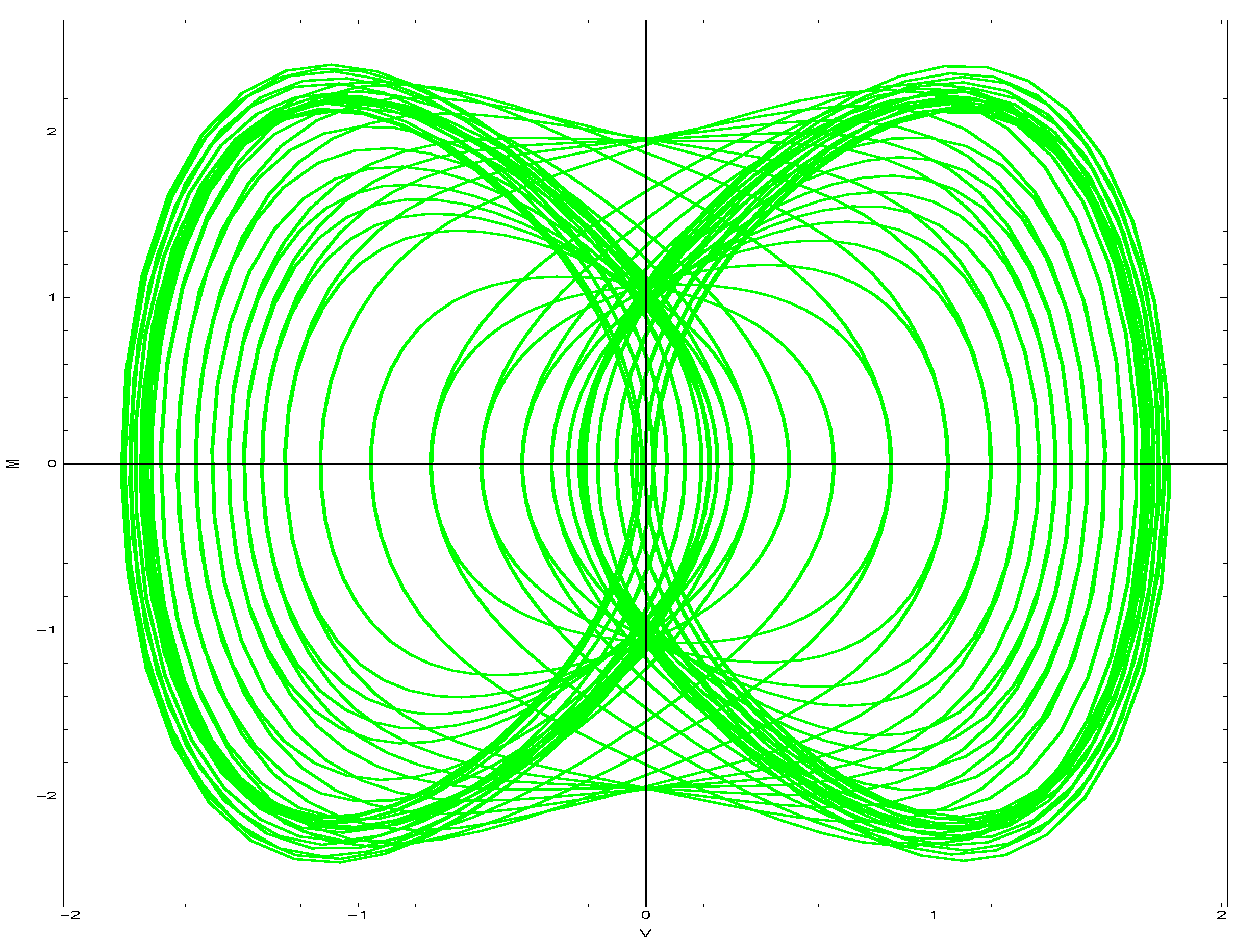
4. Chaotic Analysis

By adding a perturbation, we investigate the system’s possible chaotic tendencies in the analysis that follows, which is based on (19). We analyze the two-dimensional phase diagrams of the attained dynamical system. From (19) we have the following:

$$V^{″}\left(\varphi \right)=\left(\frac{2}{{\delta }^2{\gamma }^2-{(\sigma -\gamma )}^2}\right)V^3\left(\varphi \right)-\left(\frac{{\kappa }^2}{{\gamma }^2}\right)V\left(\varphi \right).$$

(38)

Let $V^{\prime }=\mathcal{M}$, then Equation (38) is converted into the dynamical system, as follows:

$$\begin{array}{c}\hfill \left\{\begin{array}{c}\frac{dV}{d\varphi }=\mathcal{M},\hfill \\ \frac{d\mathcal{M}}{d\varphi }=\left(\frac{2}{{\delta }^2{\gamma }^2-{(\sigma -\gamma )}^2}\right)V^3\left(\varphi \right)-\left(\frac{{\kappa }^2}{{\gamma }^2}\right)V\left(\varphi \right).\hfill \end{array}\right.\end{array}$$

(39)

We will decompose system (39) into an autonomous conservative dynamical system (ACDS), as we have the following:

$$\begin{array}{c}\hfill \left\{\begin{array}{c}\frac{dV}{d\varphi }=\mathcal{M},\hfill \\ \frac{d\mathcal{M}}{d\varphi }=\left(\frac{2}{{\delta }^2{\gamma }^2-{(\sigma -\gamma )}^2}\right)V^3\left(\varphi \right)-\left(\frac{{\kappa }^2}{{\gamma }^2}\right)V\left(\varphi \right)+m_0\cos \left(\epsilon \varphi \right),\hfill \end{array}\right.\end{array}$$

(40)

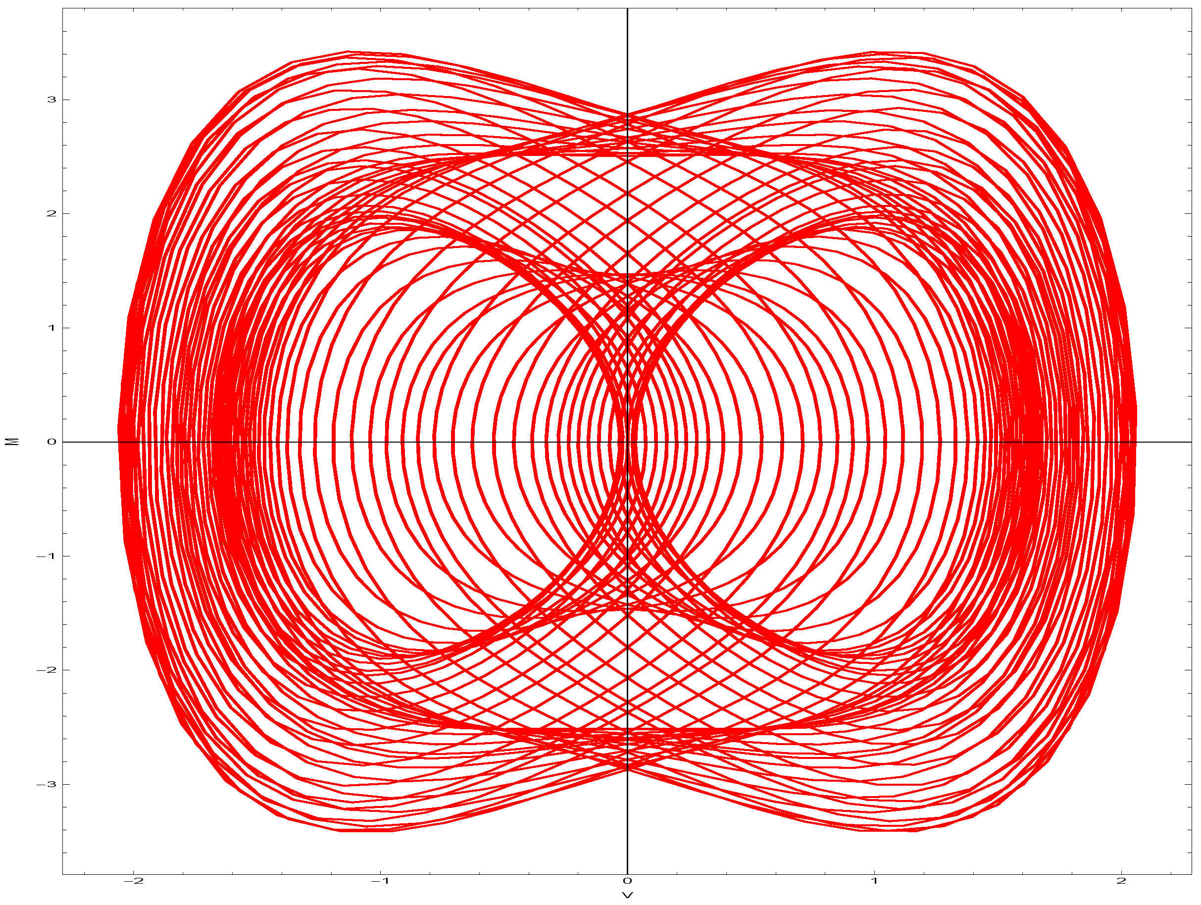
where $m_0$ represents the frequency and $\epsilon$ interprets the intensity of the perturbed factor. The two-dimensional phase graph of the dynamical system (40) utilizes different values of parameters $\gamma =0.02,\sigma =1,\delta =0.01,\kappa =0.01,m_0=3$, as shown in Figure 2 and Figure 3.

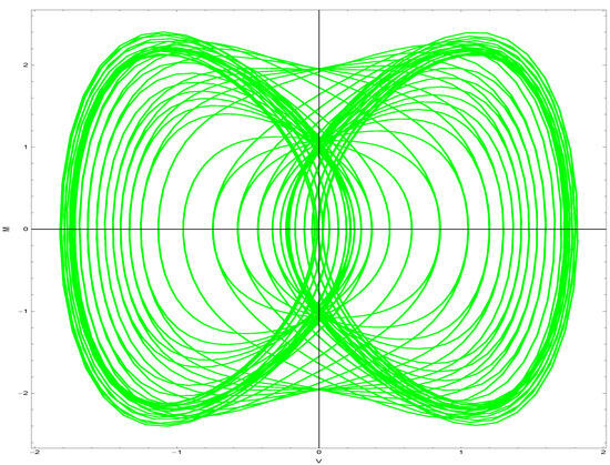
Figure 2. Phase plot of (40) with perturbed term $\epsilon =0.3$.

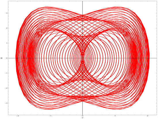
Figure 3. Phase plot of (40) with perturbed term $\epsilon =0.8$.

5. Sensitivity Analysis

Consider the following dynamical system to check the stability of the proposed model:

$$\begin{array}{c}\hfill \left\{\begin{array}{c}\frac{dV}{d\varphi }=\mathcal{M},\hfill \\ \frac{d\mathcal{M}}{d\varphi }=\left(\frac{2}{{\delta }^2{\gamma }^2-{(\sigma -\gamma )}^2}\right)V^3\left(\varphi \right)-\left(\frac{{\kappa }^2}{{\gamma }^2}\right)V\left(\varphi \right).\hfill \end{array}\right.\end{array}$$

(41)

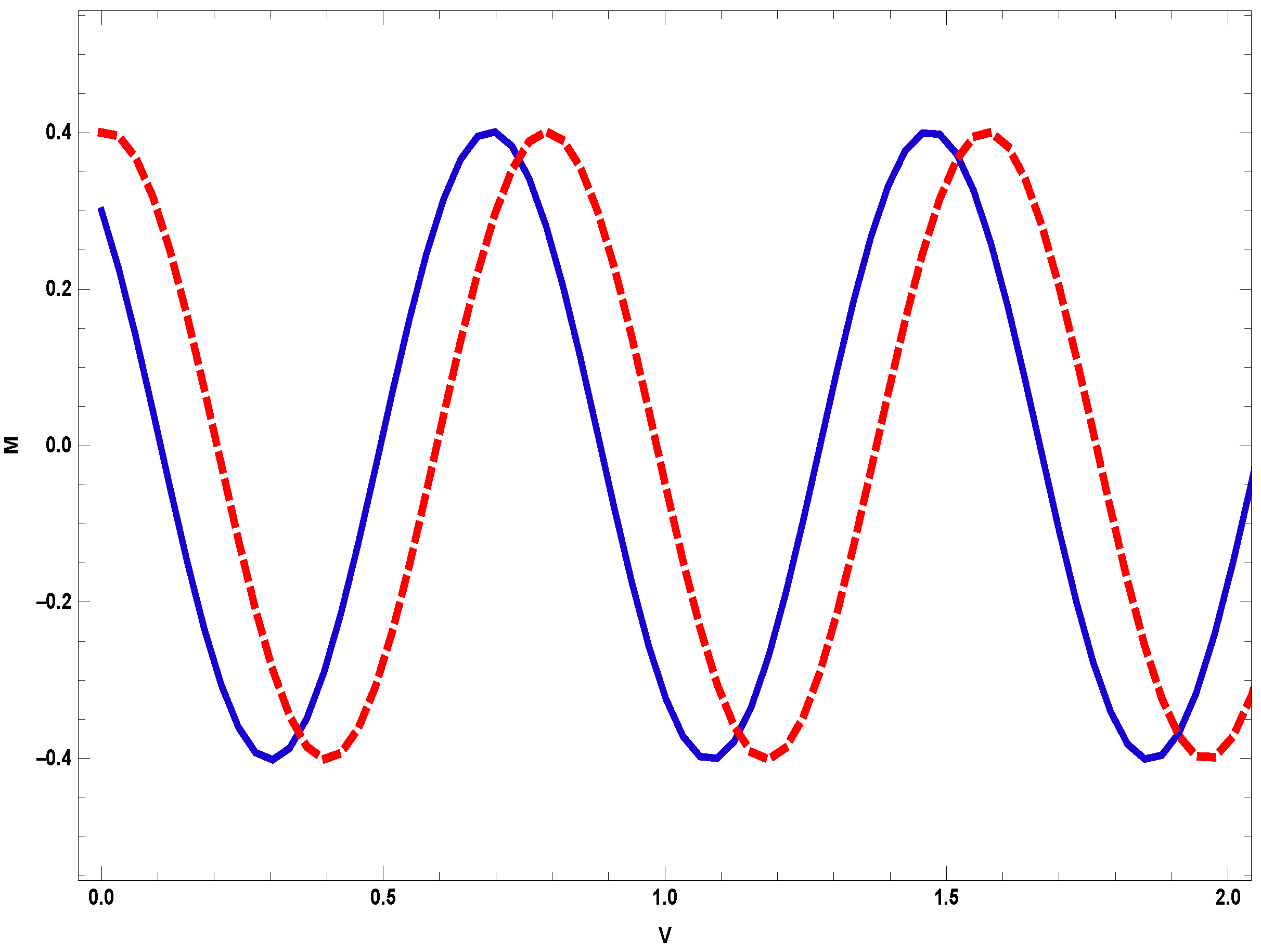
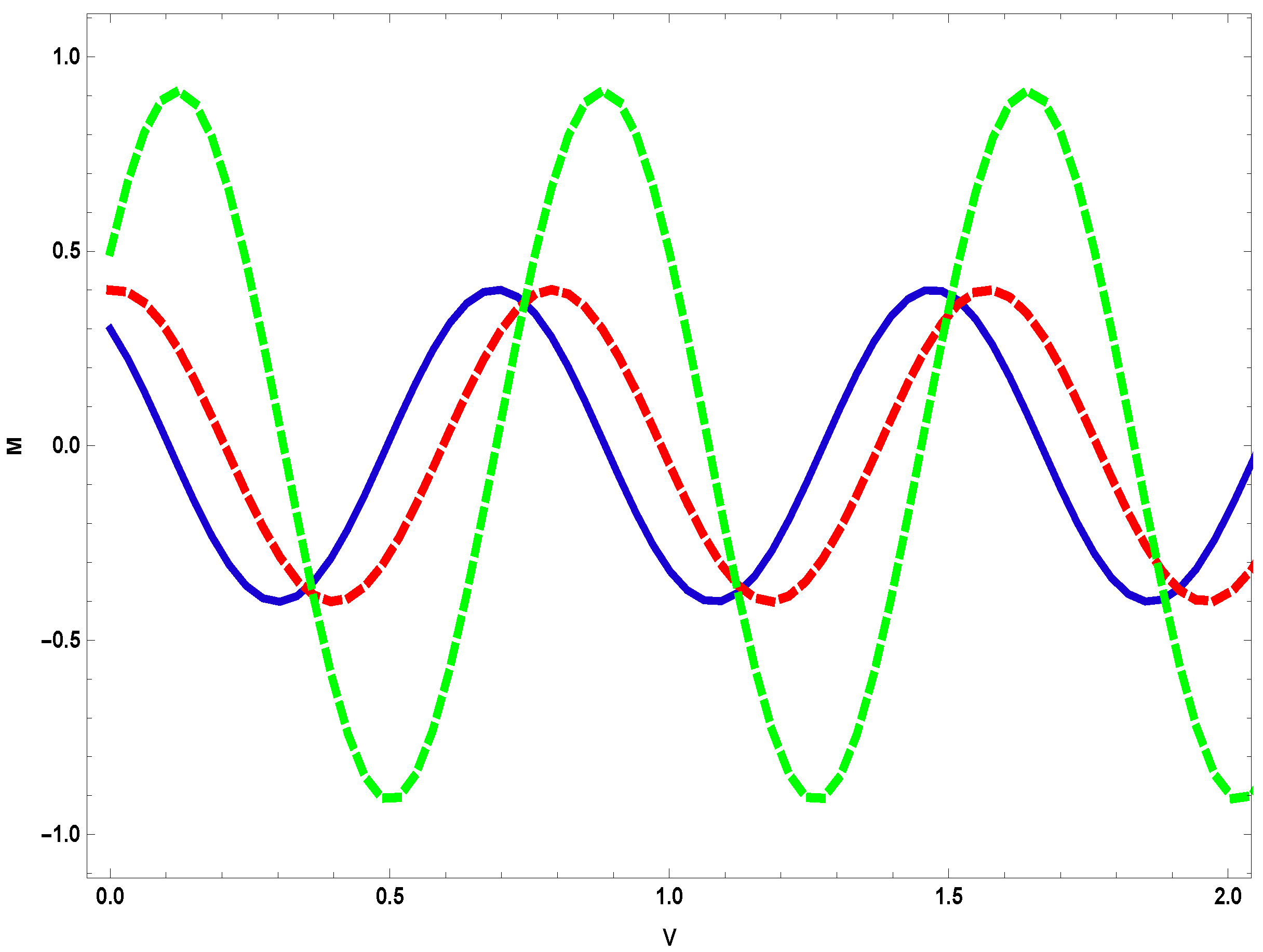
We will analyze the dynamical system (41) through the 2D plot with the help of different initial conditions and different values of parameters ($\gamma =0.02,\sigma =0.3,\delta =0.01,\kappa =0.08$). As we observe through Figure 4 and Figure 5 if we change a little bit, then there is no overlapping in the curve, so we can say that the proposed model is sensitive.

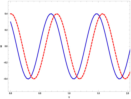
Figure 4. Sensitive analysis of dynamical system (41) for initial conditions in blue (0.3, 0) and in red (dash) (0.4, 0).

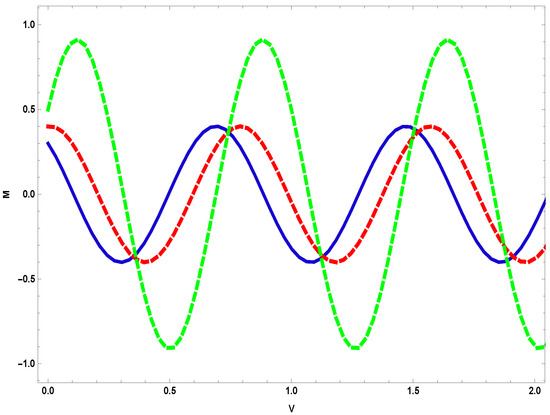
Figure 5. Sensitive analysis of dynamical system (41) for initial conditions in blue (0.3, 0), in red (dash) (0.4, 0), and green (dash) (0.5, 0).

6. Results and Discussion

The graphical representation of the NLS model solutions is covered in this section. Using Mathematica 11 to help establish appropriate values for the arbitrary constants, the physical aspect of the nonlinear model is highlighted. In [32], Tariq et al. found dark, singular, bright, and periodic soliton solutions of the NLS equation using a unified method and the simple equation method. In [30], Rafiq et al. achieved period, kink, anti-kink, and dark solutions using the unified Riccati equation expansion method and the generalized Kudryashov method. In [31], Shakeel et al. discovered various optical soliton solutions employing the generalized exponential rational function method. In the current study, we are utilizing the $\left(f+\left(\frac{G^{\prime }}{G}\right)\right)$-expansion method to find out more generalized soliton solutions.

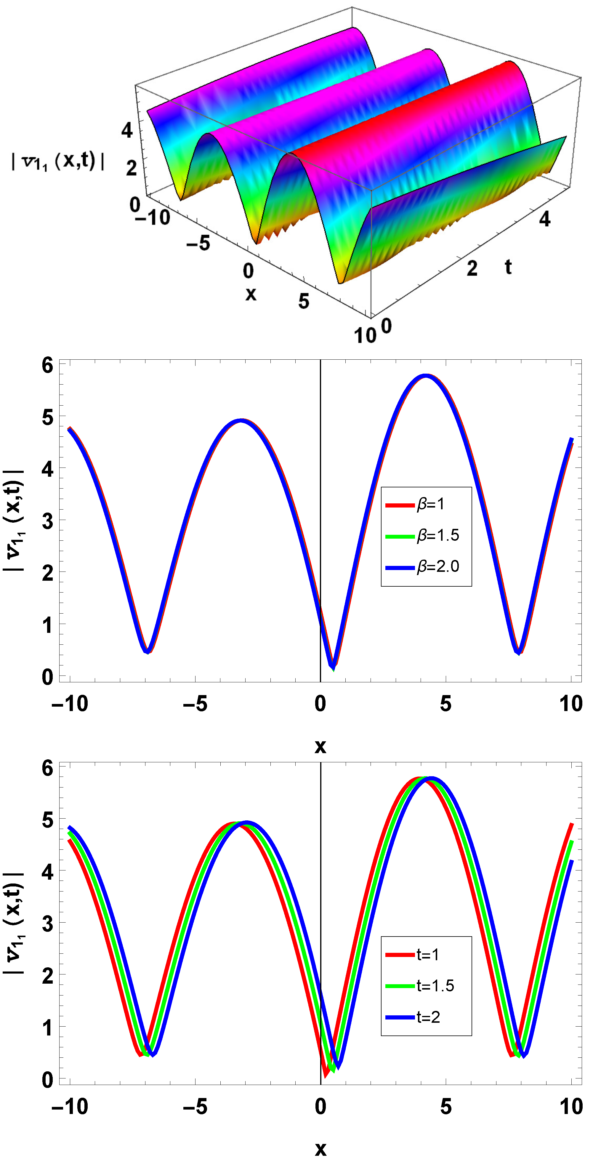
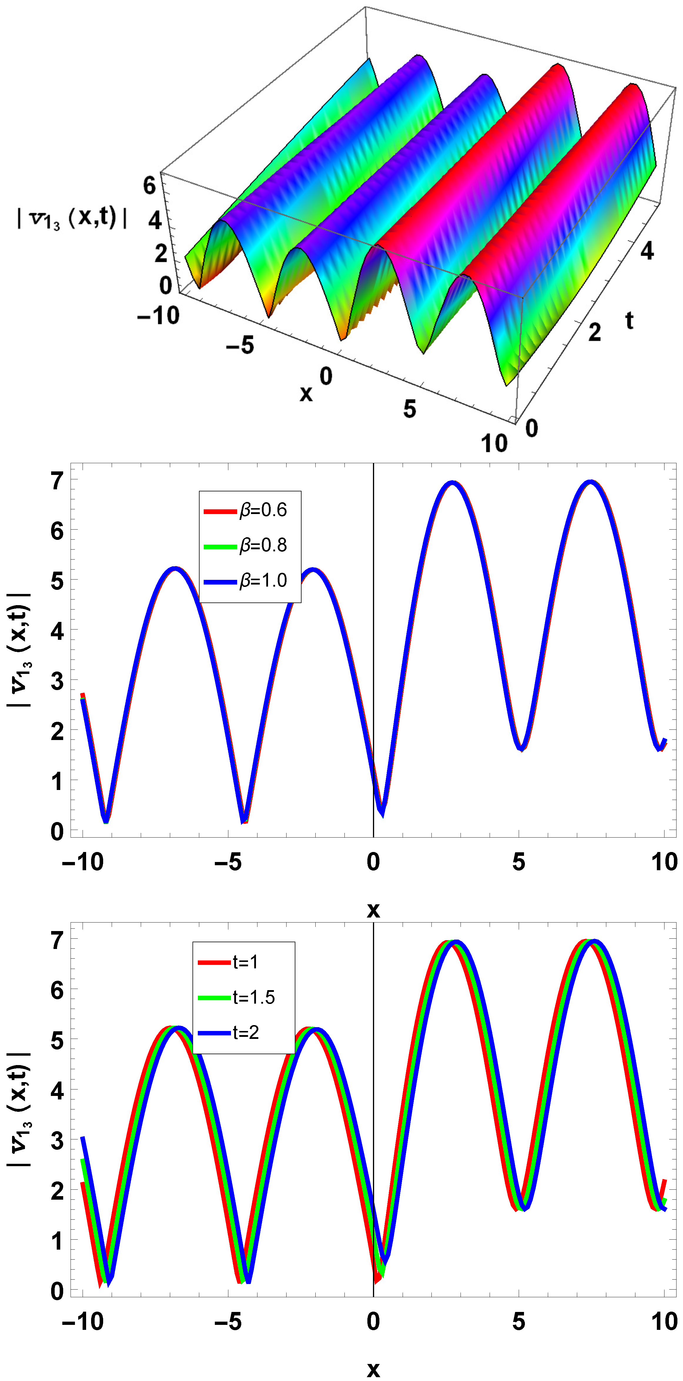
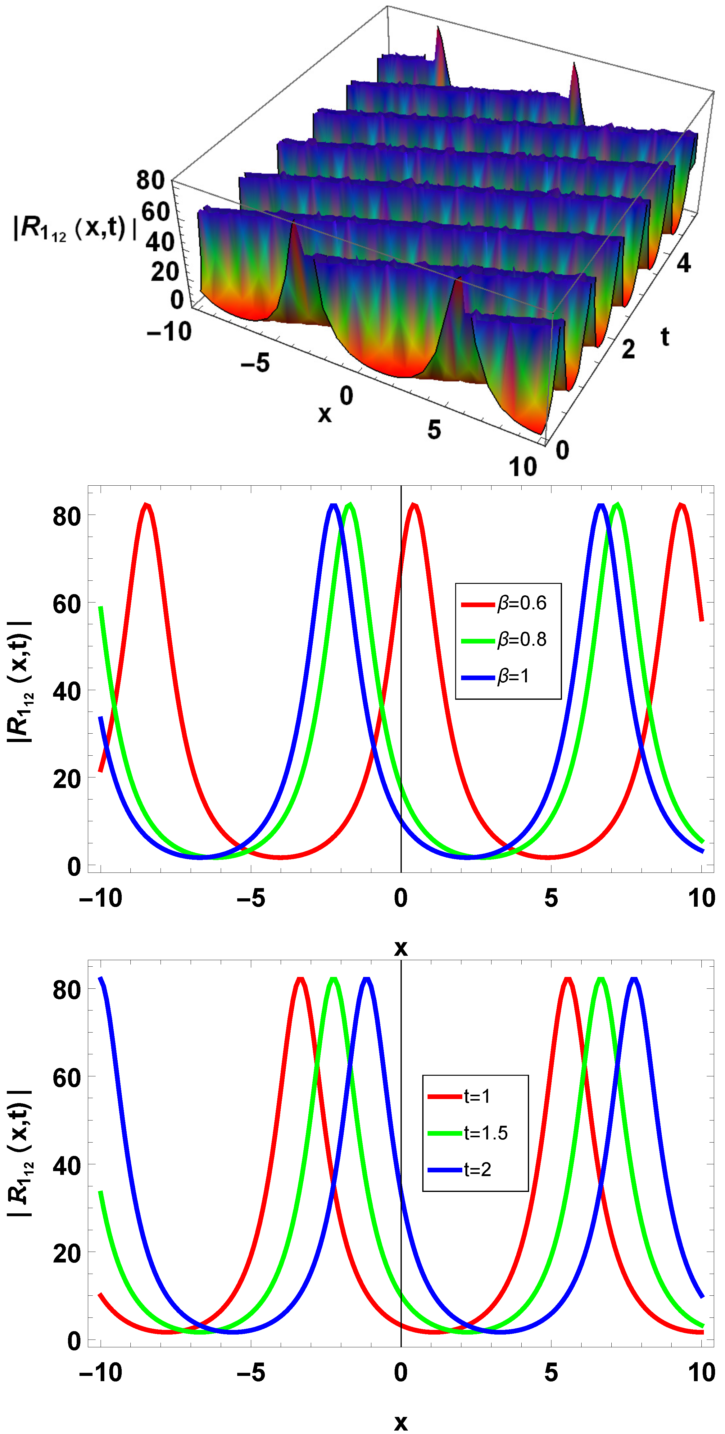
• Figure 6, Figure 7 and Figure 8 present the periodic behaviors of optical solitons. Periodic waves are repetitive disturbances that propagate through a medium at recurring intervals. These waves exhibit a consistent pattern of amplitude, frequency, and wavelength variations over time. The key aspect of periodic waves is that they regularly repeat their form after a certain interval.
  

  Figure 6. Periodic-type optical waves of (27) with parameters $\gamma =2,\sigma =0.2,\delta =0.3,f=2$, $\xi =0.2,\tau =0.2,\psi =-0.08,\xi =0.2,\omega =0.2$.
  

  Figure 7. Periodic-type optical waves of (33) with parameters $\gamma =0.8,\sigma =0.02,\delta =0.3,f=-2$, $\xi =2,\tau =0.2,\psi =-0.8,\xi =0.2,\omega =-2$.
  

  Figure 8. Singular periodic-type optical waves of (37) with parameters $\gamma =-0.5,\sigma =5,\delta =0.3$, $f=-2,\xi =-0.02,\tau =0.2,\psi =2,\xi =0.5,\omega =0.08$.
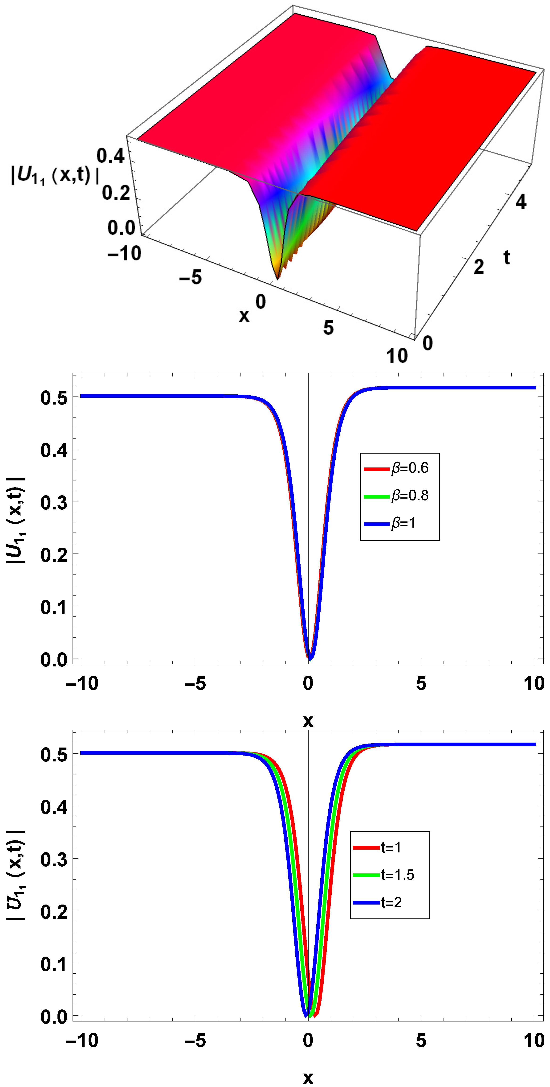
• Figure 9 shows the dark behavior of the optical soliton. In the optics, “dark waves” might refer to regions in a wave pattern with significantly lower amplitude or intensity than surrounding areas. This could happen, for example, in interference patterns where formative and destructive interference outcomes are present in regions of light and darkness.
  

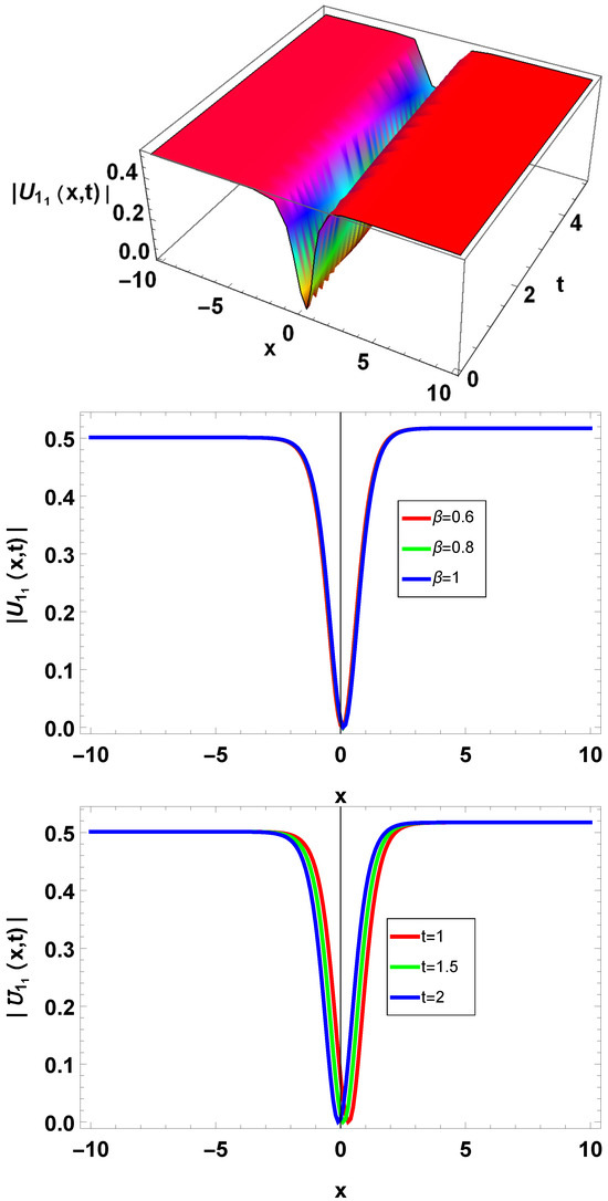  Figure 9. Dark-type optical waves of (29) with parameters $\gamma =-1,\sigma =-0.2,\delta =0.3,f=2$, $\xi =0.02,\tau =0.2,\psi =-0.08,\xi =1.5,\omega =0.02$.
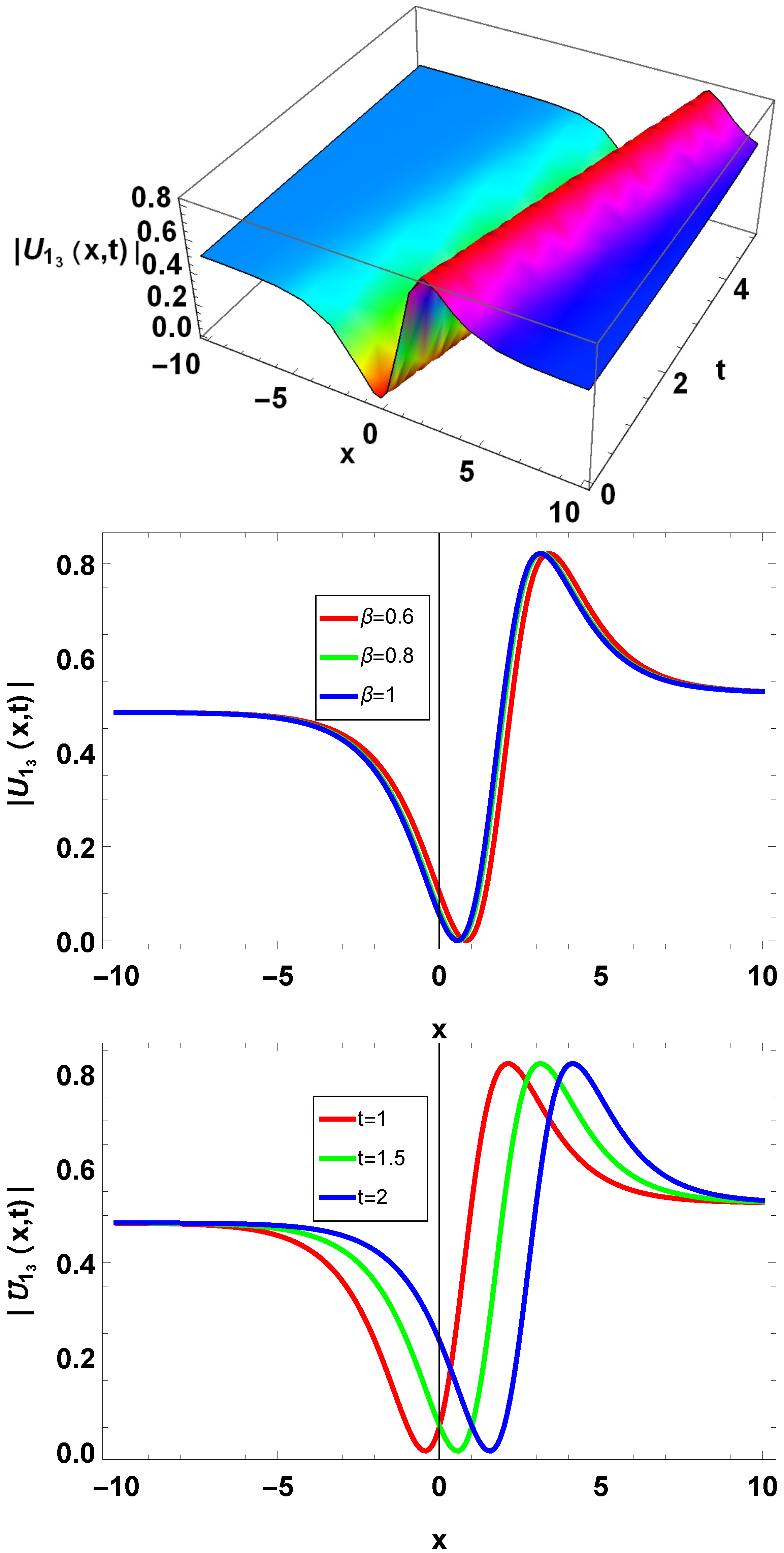
• Figure 10 and Figure 11 present the kink and anti-kink waves. Kinks are localized disturbances or “bumps” that occur within a medium. Anti-kinks are identical to kinks but illustrate transitions in the opposite approach. They also apply a sharp change in the field value (but in the opposite direction approximated to kinks). Anti-kink waves can be considered localized “dips” or “depressions” in the field profile.
  

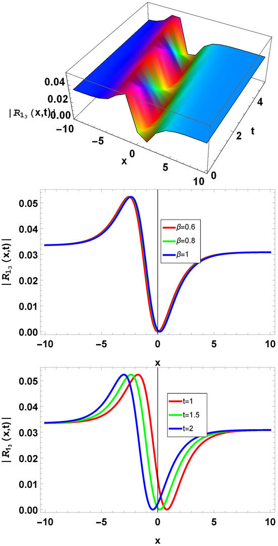  Figure 10. Kink-type optical waves of (34) with parameters $\gamma =0.8,\sigma =0.5,\delta =0.03,f=-2$, $\xi =0.02,\tau =0.2,\psi =-0.2,\xi =0.2,\omega =0.02$.
  

  Figure 11. Anti-kink-type optical waves of (35) with parameters $\gamma =-0.8,\sigma =0.8,\delta =0.3$, $f=-2,\xi =0.02,\tau =0.2,\psi =-0.2,xi=0.2,\omega =0.02$.

In the 2D graph, there is a blue line for $t=1$, a black line for $t=1.5$, a red line for $t=2$, a blue line for $\beta =1$, a black line for $\beta =0.8$, and a red line for $\beta =0.6$. In the 2D graph, we observed that when the value of t increases, amplitude decreases, and amplitude increases when the value of t decreases. Similarly, by increasing the value of the beta amplitude, it decreases; otherwise, it increases. The fractional parameter $\beta =1$ value is the same in each 3D plot.

7. Conclusions

This article described the beta derivative-based time fractional nonlinear Schrödinger model. The generalized optical soliton solutions were achieved by utilizing the $\left(m+\left(\frac{G^{\prime }}{G}\right)\right)$-expansion method for a given model, and the results were successfully verified with chaotic and sensitivity analysis. Bright, kink, anti-kink, dark, exponential, trigonometric, and hyperbolic outcomes were attained. Additionally, applications for these analytical solitary wave solutions are evident in optical fibers and communication systems. The suggested approach is vital in solving nonlinear PDEs and mathematical physics. The results show that the nonlinearities and dispersive effects can be balanced to produce solutions for solitary waves that propagate while maintaining their speed and shape.

References

- Gardner, C.S.; Greene, J.M.; Kruskal, M.D.; Miura, R.M. Method for solving the Korteweg-deVries equation. Phys. Rev. Lett. 1967, 19, 1095. [Google Scholar] [CrossRef]
- Zhou, T.; Tian, B.; Shen, Y.; Gao, X. Bilinear form, bilinear auto-Bäcklund transformation, soliton and half-periodic kink solutions on the non-zero background of a (3 + 1)-dimensional time-dependent-coefficient Boiti-Leon-Manna-Pempinelli equation. Wave Motion 2023, 121, 103180. [Google Scholar] [CrossRef]
- Ma, W.; Yong, X.; Lü, X. Soliton solutions to the B-type Kadomtsev–Petviashvili equation under general dispersion relations. Wave Motion 2021, 103, 102719. [Google Scholar] [CrossRef]
- Tang, W. Soliton dynamics to the Higgs equation and its multi-component generalization. Wave Motion 2023, 120, 103144. [Google Scholar] [CrossRef]
- Li, L.; Yu, F. The fourth-order dispersion effect on the soliton waves and soliton stabilities for the cubic-quintic Gross–Pitaevskii equation. Chaos Solitons Fractals 2024, 179, 114377. [Google Scholar] [CrossRef]
- Yao, S.W.; Zafar, A.; Urooj, A.; Tariq, B.; Shakeel, M.; Inc, M. Novel solutions to the coupled KdV equations and the coupled system of variant Boussinesq equations. Results Phys. 2023, 45, 106249. [Google Scholar] [CrossRef]
- Russel Scott, J. Report of waves. In Report of the 14th Meeting of the British Association for the Advancement of Science; Scientific Research: London, UK, 1844; pp. 311–390. [Google Scholar]
- Nguepjouo, F.T.; Kuetche, V.K.; Kofane, T.C. Soliton interactions between multivalued localized waveguide channels within ferrites. Phys. Rev. E 2014, 89, 063201. [Google Scholar] [CrossRef]
- Khater, A.H.; Callebaut, D.K.; Seadawy, A.R. General soliton solutions of an n-dimensional complex Ginzburg–Landau equation. Phys. Scr. 2000, 62, 353. [Google Scholar] [CrossRef]
- Khater, A.H.; Seadawy, A.R.; Helal, M.A. General soliton solutions of an n-dimensional nonlinear Schrödinger equation. Nuovo Cimento B 2000, 115, 1303–1311. [Google Scholar]
- Liu, S.; Fu, Z.; Liu, S.; Zhao, Q. Jacobi elliptic function expansion method and periodic wave solutions of nonlinear wave equations. Phys. Lett. A 2001, 289, 69–74. [Google Scholar] [CrossRef]
- Rady, A.A.; Osman, E.S.; Khalfallah, M. The homogeneous balance method and its application to the Benjamin–Bona–Mahoney (BBM) equation. Appl. Math. Comput. 2010, 217, 1385–1390. [Google Scholar]
- Ali, A.; Seadawy, A.R.; Lu, D. Soliton solutions of the nonlinear Schrödinger equation with the dual power law nonlinearity and resonant nonlinear Schrödinger equation and their modulation instability analysis. Optik 2017, 145, 79–88. [Google Scholar] [CrossRef]
- Ali, A.; Seadawy, A.R.; Lu, D. Computational methods and traveling wave solutions for the fourth-order nonlinear Ablowitz-Kaup-Newell-Segur water wave dynamical equation via two methods and its applications. Open Phys. 2018, 16, 219–222. [Google Scholar] [CrossRef]
- Osman, M.S.; Zafar, A.; Ali, K.K.; Razzaq, W. Novel optical solitons to the perturbed Gerdjikov–Ivanov equation with truncated M-fractional conformable derivative. Optik 2020, 222, 165418. [Google Scholar] [CrossRef]
- Khater, M.M.; Lu, D.; Attia, R.A. Dispersive long wave of nonlinear fractional Wu-Zhang system via a modified auxiliary equation method. AIP Adv. 2019, 9, 025003. [Google Scholar] [CrossRef]
- Akbulut, A.; Kaplan, M. Auxiliary equation method for time-fractional differential equations with conformable derivative. Comput. Math. Appl. 2018, 75, 876–882. [Google Scholar] [CrossRef]
- Younis, M.; Iftikhar, M. Computational examples of a class of fractional order nonlinear evolution equations using modified extended direct algebraic method. J. Comput. Methods Sci. Eng. 2015, 15, 359–365. [Google Scholar] [CrossRef]
- Ahmad, S.; Salman; Ullah, A.; Ahmad, S.; Akgül, A. Bright, dark and hybrid multistrip optical soliton solutions of a non-linear Schrödinger equation using modified extended tanh technique with new Riccati solutions. Opt. Quantum Electron. 2023, 55, 236. [Google Scholar] [CrossRef]
- Zafar, A.; Shakeel, M.; Ali, A.; Rezazadeh, H.; Bekir, A. Analytical study of complex Ginzburg–Landau equation arising in nonlinear optics. J. Nonlinear Opt. Phys. Mater. 2023, 32, 2350010. [Google Scholar] [CrossRef]
- Ma, H.; Mao, X.; Deng, A. Interaction solutions for the (2 + 1)-dimensional extended Boiti-Leon-Manna-Pempinelli equation in incompressible fluid. Commun. Theor. Phys. 2023, 75, 085001. [Google Scholar] [CrossRef]
- Biswas, S.; Ghosh, U.; Raut, S. Construction of fractional granular model and bright, dark, lump, breather types soliton solutions using Hirota bilinear method. Chaos Solitons Fractals 2023, 172, 113520. [Google Scholar] [CrossRef]
- Jumarie, G. Modified Riemann-Liouville derivative and fractional taylor series of nondifferentiable functions further results. Comput. Math. Appl. 2006, 51, 1367–1376. [Google Scholar] [CrossRef]
- Podlubny, I. An introduction to fractional derivatives, fractional differential equations, to methods of their solution and some of their applications. Math. Sci. Eng. 1999, 198, 340. [Google Scholar]
- Wang, K.-L. A novel computational approach to the local fractional lonngren wave equation in fractal media. Math. Sci. 2023, 1–6. [Google Scholar] [CrossRef]
- Yepez-Martinez, H.; Gómez-Aguilar, J. Optical solitons solution of resonance nonlinear Schrödinger type equation with Atangana’s-conformable derivative using sub-equation method. Waves Random Complex Media 2021, 31, 573–596. [Google Scholar] [CrossRef]
- Almeida, R. A Caputo fractional derivative of a function with respect to another function. Commun. Nonlinear Sci. Numer. Simul. 2017, 44, 460–481. [Google Scholar] [CrossRef]
- Atta, D. Thermal diffusion responses in an infinite medium with a spherical cavity using the Atangana-Baleanu fractional operator. J. Appl. Comput. Mech. 2022, 8, 1358–1369. [Google Scholar]
- Ablowitz, M.J.; Prinari, B.; Trubatch, A.D. Discrete and Continuous Nonlinear Schrödinger Systems; Cambridge University Press: Cambridge, UK, 2004; Volume 302. [Google Scholar]
- Rafiq, M.H.; Jannat, N.; Rafiq, M.N. Sensitivity analysis and analytical study of the three-component coupled NLS-type equations in fiber optics. Opt. Quantum Electron. 2023, 55, 637. [Google Scholar] [CrossRef]
- Shakeel, M.; Bibi, A.; AlQahtani, S.A.; Alawwad, A.M. Dynamical study of a time fractional nonlinear Schrödinger model in optical fibers. Opt. Quantum Electron. 2023, 55, 1010. [Google Scholar] [CrossRef]
- Tariq, K.U.; Nadeem, M.; Zeeshan, M.; Guran, L.; Bucur, A. On the dynamics of a dual space time fractional nonlinear Schrödinger model in optical fibers. Results Phys. 2023, 51, 106603. [Google Scholar] [CrossRef]
Disclaimer/Publisher’s Note: The statements, opinions and data contained in all publications are solely those of the individual author(s) and contributor(s) and not of MDPI and/or the editor(s). MDPI and/or the editor(s) disclaim responsibility for any injury to people or property resulting from any ideas, methods, instructions or products referred to in the content. |
© 2024 by the authors. Licensee MDPI, Basel, Switzerland. This article is an open access article distributed under the terms and conditions of the Creative Commons Attribution (CC BY) license (https://creativecommons.org/licenses/by/4.0/).