Abstract
This study proposes an enhanced Kepler Optimization (EKO) algorithm, incorporating fractional-order components to develop a Proportional-Integral-First-Order Double Derivative (PI–(1+DD)) controller for frequency stability control in multi-area power systems with wind power integration. The fractional-order element facilitates efficient information and past experience sharing among participants, hence increasing the search efficiency of the EKO algorithm. Furthermore, a local escaping approach is included to improve the search process for avoiding local optimization. Applications were performed through comparisons with the 2020 IEEE Congress on Evolutionary Computation (CEC 2020) benchmark tests and applications in a two-area system, including thermal and wind power. In this regard, comparisons were implemented considering three different controllers of PI, PID, and PI–(1+DD) designs. The simulations show that the EKO algorithm demonstrates superior performance in optimizing load frequency control (LFC), significantly improving the stability of power systems with renewable energy systems (RES) integration.
1. Introduction
Reducing environmental impacts as the world moves towards more environmentally friendly and green power options requires the integration of RESs. Frequency fluctuations result from these renewable sources’ unpredictability, which puts strain on power networks’ stability. With the increasing scale of wind power integration, LFC has become a critical challenge for power systems. The intermittency and instability of wind power impose higher demands on the frequency stability of power systems, making the development of effective control strategies to address these challenges particularly important [1]. As an illustration of the evolving landscape, recent research has highlighted a gradual decrease in inertia across Europe, showing a decline of approximately 20% over the past two decades [2]. Highlighting the intricacies of this changing dynamic, an incident occurred in the Southern California System on 16 August 2016, where a disruption of 1200 MW of solar generation took place. This event was triggered by a low-inertia condition, leading to the activation of inverter protections based on instantaneous frequency measurement [3]. Similarly, in 2019, the UK experienced a significant power outage lasting 1.5 h, resulting in a 5% loss of total load [4]. In light of these occurrences, the traditional hierarchical control scheme, encompassing primary, secondary, and tertiary frequency control, appears inadequate in ensuring dynamic security if the power system continues to transition towards increasing reliance on RES [5].
Sustaining the equilibrium between generation and demand for power requires a well-executed LFC strategy [6]. The stability of a whole electricity grid depends on this balance. Through the efficient handling of frequency irregularities brought about by the incorporation of RESs, electrical power networks develop more resilience and adaptability, which in turn add to the long-term sustainability and dependability of the world’s energy infrastructure. Hit-and-trial assessment with various loads and controllers, comprising I, PI, and PID, was used in [7] to apply I, PI, and PID control strategies in order to preserve the steady frequencies in each region. In reference [8], a PI-controller that can be used for LFC in multi-area systems was reported. It was created utilizing a restricted population extreme optimizer. Three distinct models of two-area power systems were used as test cases to illustrate the efficacy of the designed controller. One drawback of the model was that nonlinear components were not taken into consideration by the state space model used in this method. Also, a method based on Harris Hawks’ algorithm was created by [9] in designing a PI controller to address issues related to frequency-associated concerns. This plan was examined using a range of standard benchmark tools to address different optimization issues. An adaptive LFC technique for power systems was presented in [10], which involved employing an electro-search optimizer to regulate the integral controller’s settings. Nevertheless, the system’s objective function was developed without taking into account variations in the system’s parameters or load disruptions, instead relying solely on the power plant’s transfer function. Consequently, inappropriate performance under load fluctuations and changes in system characteristics could arise from this approach. The cascaded tilt–integral–derivative controller was tuned by using the Salp Swarm Algorithm for LFC control and elucidated by Ref. [11]. Utilizing the benefits of the cascade controller in conjunction with fractional-order elements, the executed control method via TID controller, the slave, and the PI controller, the master was comparative assessed against differential evolution and flower pollination algorithms.
RESs are thought to be the most effective and environmentally friendly technologies, especially wind energy. The cost of their upkeep and operations has dramatically dropped recently. By incorporating multiple RESs, such as solar systems, turbines, and possibly diesel generating units for backup, hybrid power sources serve a critical role in guaranteeing a steady energy supply [12]. As a result, combining these hybrid plants with conventional power plants improves their ability to handle efficient loads overall. Reference [13] delves into the stability analysis of a multi-WTs system, albeit without extending the findings to multi-area power systems. On the other hand, Ref. [14] discusses a control strategy tailored to variable-speed WTs within the Argentine–Uruguayan grid, yet it focuses solely on an on–off scheme applied to a single-area power system. Furthermore, Ref. [15] offers an exhaustive categorization of SI control techniques in power systems with a high penetration of renewables, though concentrating primarily on the control technique rather than the power system model. In [16], a contemporary methodology was introduced for automatic LFC in multiple-source power systems, utilizing PID control tuned by a hybrid technique of sparrow optimization and bald eagle algorithm. In this work, the hybrid algorithm leverages the dynamic characteristics associated with bald eagles and sparrows to address convergence issues commonly encountered in optimization problems. Then, again, Ref. [17] provides inertial responsiveness and conducts a modal study using the reserves of both kinetic and electrostatic energies of the rotor from variable-speed WT and the supercapacitor units, respectively. The implemented control strategy was not thoroughly explained, and the power system representation utilized throughout the investigation was constructed on a condensed two-area testing system. Moreover, only the power system’s frequency was utilized as a feedback variable, thereby imposing a limitation on the scope of analysis. Table 1 summarizes a comparative analysis of the present work with the existing state-of the-art.

Table 1.
Summary of existing state-of-the-art compared to the presented work considering a two-area system.
The existing literature on LFC in power systems, particularly with the integration of RESs, reveals several significant shortcomings that have motivated further research. Firstly, a notable issue is the inadequate handling of nonlinear components in many control models. This limitation can result in suboptimal performance, particularly under varying load conditions and dynamic system behavior. Another critical shortcoming is the lack of adaptability to load fluctuations and system parameter variations. This oversight can lead to inappropriate performance when the system encounters real-world conditions where load demands and characteristics frequently change. Additionally, the integration of hybrid renewable sources with conventional power plants is not comprehensively addressed in the existing research. While studies like References [13,14] explore specific scenarios involving wind turbines, they do not extend their findings to multi-area power systems or consider the combined dynamics of multiple RESs and traditional energy sources. This gap highlights the need for control strategies that effectively manage the diverse and hybrid nature of modern power grids. Handling LFC in multi-area power grids requires the use of increasingly sophisticated controllers and effective algorithms. In this instance, M. Abdel-Basset et al. [25] recently presented KO, a revolutionary physics-based algorithm influenced by Kepler’s equations explaining the orbits of the planets. KO offers a special version of the metaheuristic for estimating the planet’s position and velocity at a given time that is based on Kepler’s computations [26]. In KO, each planet serves as a possible solution that is arbitrarily adjusted during the process of optimization with regard to the Sun to determine the best possible future solution. To address the LFC problem, this paper presents a ground-breaking augmented EKO with additional fractional-order components in order to design an advanced controller based on PI–(1+DD) stages. To boost the search efficiency of the EKO, the primarily engaged change employs a fractional-order element to achieve effective information and past expertise sharing amongst participants with the goal of avoiding premature converging. Additionally, the LEA was incorporated to boost the search procedure by evading local optimization. A two-area electrical system with a thermal plant and wind renewable energy source was used to describe the LFC problem. It was vulnerable to successive random variations and varying load demands in every area. Minimization of the ITAE was the time domain objective function assessed and investigated. The present study offers the following significant contributions:
- An EKO algorithm enhanced with additional fractional-order components is presented.
- An advanced PI–(1+DD) controller, based on EKO, is introduced to enhance frequency stability in multi-area power systems with wind integration.
- The performance of the proposed controller is investigated, showcasing significant enhancements considering simultaneous step load changes in both thermal and wind areas.
- The proposed EKO algorithm is comprehensively evaluated and compared against several recent algorithms.
2. Two-Area Power System with WTG
2.1. Wind Farm
Wind power generation is inherently unpredictable, owing to its dependency on external factors such as wind speed, ambient temperature, and more. The electricity output of wind farms is significantly influenced by the continuous variation in wind speeds over the course of the day. The mathematical modeling of the mechanical power output from a wind turbine (PGW) is represented as follows [27]:
In this context, the parameter “a” is defined as the swept area, measured in square meters (m2); “ρ” represents the air density, measured in kilograms per cubic meter (kg/m3); “Vw” stands for the wind speed, measured in meters per second (m/s); “Cp” denotes the rotor efficiency; “β” refers to the pitch angle of the blade, measured in degrees; and “Tip” stands for the tip speed ratio. These parameters are determined by the following equations:
The parameter “Rpm” denotes the rotor speed in revolutions per minute, and “Dm” represents the diameter of the rotor blades in meters.
The pitch control is utilized to regulate the power output of the WTG. It aims to maintain the blade’s angle in an optimal way for adjusting to changes in wind speed. The input signal to the pitch controller is derived from the feedback signal of the WTG output power. The pitch control system of the wind farm, along with the data-fit pitch response, hydraulic pitch actuator, and induction generator, are all represented using transfer functions. These functions are explained sequentially as follows [22]:
where KP1, KP2, KP3, TP1, TP2, and TP3 correspond to the pitch controls, hydraulic pitch actuators, and data-fit pitch response’s gain and time constants, respectively.
The variance in wind output power is articulated as follows:
where KPC and Kf are the gains in blade characteristic and fluid coupling, respectively.
2.2. Thermal System
The thermal generation area consists of several components including the turbine, governor, re-heater, and generator. Below, each of their transfer functions is detailed sequentially [28].
where Kg, Tg, Kt, Tt, Kr, Tr, Kp, and Tp indicate the thermal plant governor, turbine, reheater, and power system’s gain and time constants, respectively. The controllers receive inputs in the form of related area control errors (ACE1 and ACE2), which are defined as follows:
The model of the power system under investigation is depicted in Figure 1. In this figure, R denotes the governor speed droop characteristics; B refers to the frequency bias factor; PL indicates the nominal thermal loading; ∆PD1 and ∆PD2 are the power demand changes in both areas; ∆Pw refers to the wind power fluctuations; ∆PTIE is the tie-line power change; T12 constitutes the synchronization coefficient of the tie-line; ∆fl and ∆f2 are the frequency deviations (Hz) in both areas.
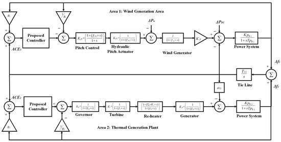
Figure 1.
Power system model.
3. Proposed Controller-Based Enhanced Kepler Optimization (EKO)
3.1. Proposed PI–(1+DD) Controller
In this investigation, we utilize a controller fashioned by using PI–(1+DD) to regulate frequency fluctuations, showcasing its superior efficacy when juxtaposed with traditional controllers [29]. The foundational layout of the envisaged PI–(1+DD) controller is depicted in Figure 2. As depicted in the figure, the controller is structured into two tiers, namely PI and DD. Additionally, the architecture of the PI–(1+DD) controller incorporates two independently adjustable parameters, KP and KI, on one side, and KD1, KD2 alongside a constant gain of 1 on the other side. The adjustable parameters afford flexibility in controller customization. The merits of the proposed PI–(1+DD) controller include augmented transient response and heightened system stability, culminating in a decrease in peak deviation. The transfer function of the envisaged controller is delineated in Equation (15).
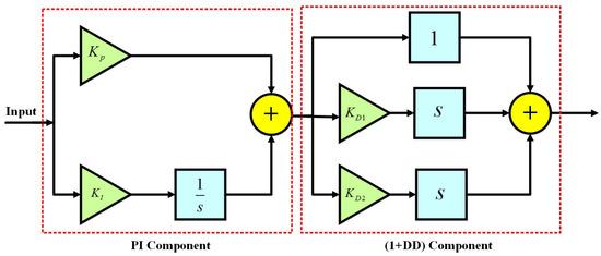
Figure 2.
Proposed controller of PI–(1+DD) [29].
In LFC analyses, the optimization of different controllers is carried out using the integral of ITAE as the performance index. Equation (16) defines the ITAE minimization function utilized for this particular objective.
To enhance system responsiveness, it is crucial to minimize the J value, taking factors such as ∆f1, ∆f2, and ∆PTIE into account within the time span of tsim. The only exception is the boundary for the filter coefficient n of the PID controller, which is set between 1 and 200, while all other candidate controller parameters are adjusted within the range of −4 to 4 [22].
3.2. Developing EKO for Tunning the Proposed Controller
KO provides an exclusive meta-heuristic description of the field of physics-based inspiration, relying on Kepler’s calculations to anticipate the velocity and position of the planets at specific moments [25]. This section presents a ground-breaking EKO with additional fractional-order components. The EKO algorithm introduces an information-sharing mechanism and an LEA, effectively improving search efficiency and avoiding premature convergence. Specifically, the information-sharing mechanism allows individuals to exchange information during the optimization process, thereby finding the global optimum more quickly, while the LEA method helps individuals escape local optima, enhancing the algorithm’s global search capability [30].
3.2.1. Primary Addition of Fractional-Order Element
The concept of fractional calculus is frequently centered on GL calculation, which can be mathematically expressed in the following manner [31]:
where
where Dζ(x(t)) represents the fractional derivative with order ζ of the Grunwald–Letnikov formula and Obi(t) becomes the solution vector, defining each object’s position in space at every point in time (t). Γ finds the gamma function. The following equation represents its mathematical structure for discrete-time execution:
where T is the sample interval. Equation (19) is written as follows when ζ = 1: wherein D1[x(t)] denotes the variance between two-tailed occurrences.
Concerning Equation (17), it can be expressed as follows when ζ = 1:
wherein D1[Obi(t)] denotes the variance between two-tailed occurrences.
To incorporate the fractional-order element that was previously stated inside the KO, the variance between the newly generated and current position of each object can be mathematically simulated as follows:
On the basis of the suggested framework, the stored information and heredity portions of the motivated action are defined in the method to speed up the exploration approach. When changing its placement according to the combination approach, every alternative solution vector uses memory, and the updated position of each object can be simplified and estimated as follows:
As stated in Equation (22), if the present iteration surpasses three, this method accomplishes nothing extra. This characteristic is caused by the reliance on prior recollections.
3.2.2. Proposed EKO
The Sun is regarded as the most favorable or best option in KO, whereas the placements of the different planets constitute potential alternatives that arbitrarily alter throughout the iterated process. The algorithm’s core equation states that upon initialization, each position (Obj) of each object (j) is randomly assigned.
where the planet population is denoted by NOb, and the minimum and maximum restrictions on every controlling variable (i), accordingly, are represented by ObL and ObU. Rd1 stands for a number that is generated at random and ranges from 0 to 1.
Then, based on the location of each object in reference to the Sun, its rate of motion is established. The aforementioned motion sequence can be represented by an algebraic equation as follows:
where
where Vk(t) signifies the object’s velocity at time t; A vector type is denoted by the symbol (→) on the tag for every element. q, q1, and q2 are integers frequently picked at random from the spectrum [0, 1]; α designates a randomized value within the range [−1, 1]; Rd1: Rd5 are numbers that are irregularly dispersed within the bounds of [0, 1]; Oba and Obb are the positions of two randomly planets; MS and mk represent the masses of the Sun regarding the best position of the planets and each object, correspondingly; μ(t) reflects the gravitational constant of the universe; ε is still a tiny amount used to avoid division by zero inaccuracies; Rk(t) corresponds to the distance between the Sun and each object; ak represents the semimajor axis of the elliptical orbit of the planet as follows:
where Tk is an absolute value derived using a normal distribution, indicating the orbital period of each object. Rk−rm(t) is the normalized Euclidian distance between the Sun and each object. Planets orbit the Sun, rotating in and out of orbit [26]. The KO concept divides the process into two phases: exploration and exploitation. Nearer solutions are used, while far-off solutions are investigated for novel possibilities.
where Obk(t + 1) represents a planet’s ultimately determined location at time t + 1; ObS(t) represents the Sun’s position with respect to the specified best solution and acts as a marker to modify the search’s orientations. The term “Fgk” refers to the force of gravity that pulls planets towards the Sun:
where μ symbolizes a gravitational constant; ei is a stochastic randomized number denoting the eccentricity of a rotating planet; and MnS and mnk stand for the normalized amounts of Mn and mk [25]. Furthermore, Rnk symbolizes the Rk’s normalized value, representing the Euclidian distance between the object and the Sun as follows:
When the planets tend to be in proximity to the Sun, KO will prioritize taking advantage of exploitation over exploring, as shown below:
where Rd7 and Rd8 represent values selected at random according to normal distribution, and a2 represents a periodic regulating factor that slowly decreases from 1 to 2 for T cycles throughout the optimizing procedure, as shown below:
Elitism, the final phase, adopts an elitist method to ensure the optimal locations for the Sun and planets. This process is outlined in the following equation:
Also, an LEA is incorporated to boost the searching procedure by evading local optimization, wherein the positions of some planets can be modified in each iteration as follows:
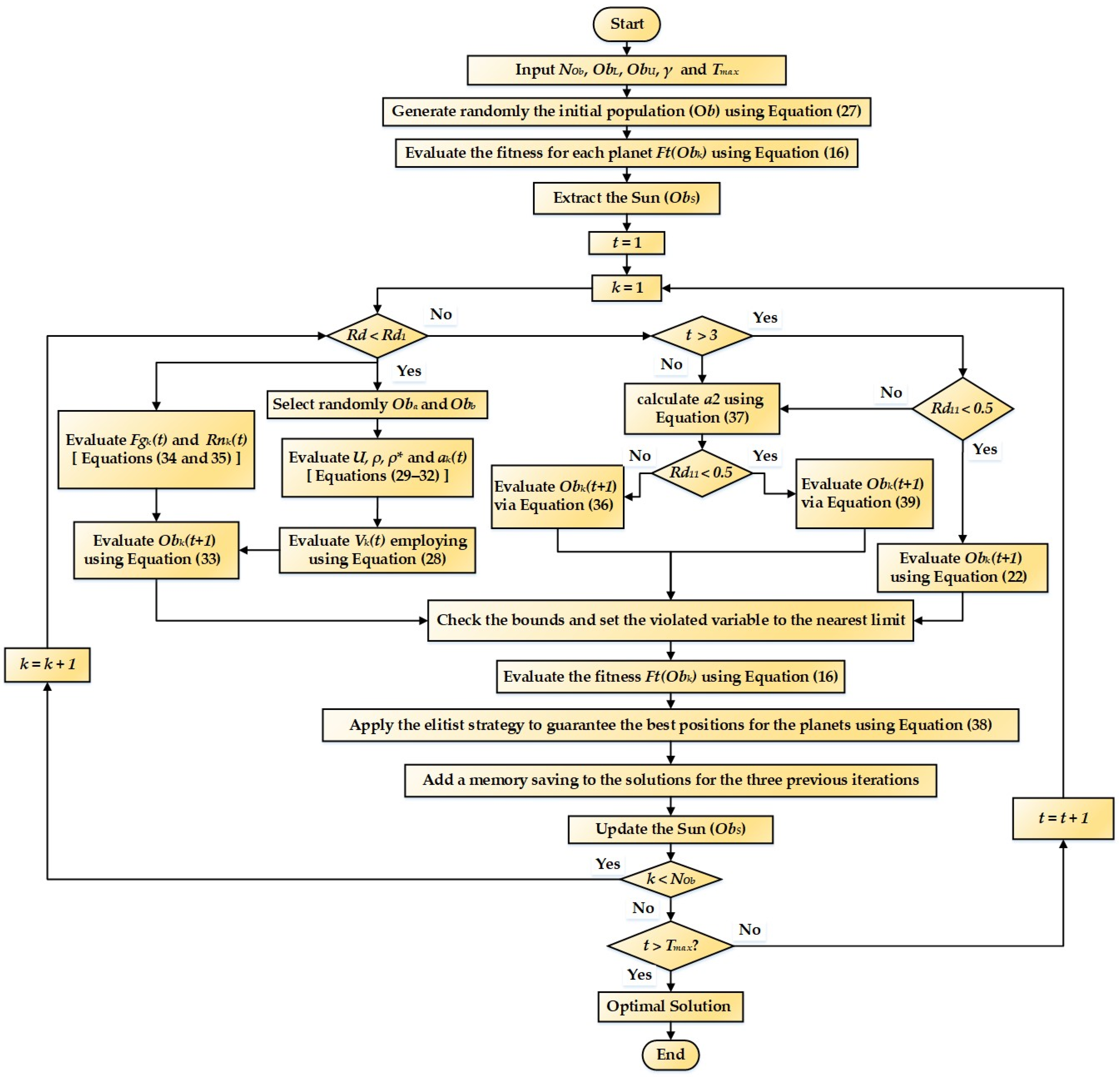
where Qw is a probability parameter that governs LEA stimulation. In the range [0, 1], Rd9 and Rd10 denote arbitrary numbers; ϕ1 and ϕ2 are random values within band [−1; 1]; Oba, Obb and Obc denote multiple solutions that were randomly selected. Also, σ1, β1, and β2 are randomized number produced in an adaptive way as in [30]. Figure 3 displays the flowchart of the proposed EKO.

Figure 3.
Flowchart of the proposed EKO.
4. Results and Discussion
4.1. Testing on RW Engineering Design Issues
Simulation results of RW problems were conducted to assess the performance of the proposed EKO algorithm in addressing constrained, non-convex optimization challenges. Thirteen optimization problems from mechanical and chemical engineering fields, drawn from CEC 2020, were utilized for testing purposes. The lower and upper limit violations of the constraint functions were determined based on reference [32].
4.1.1. Proposed EKO versus KO: Testing on RW Engineering Design Issues
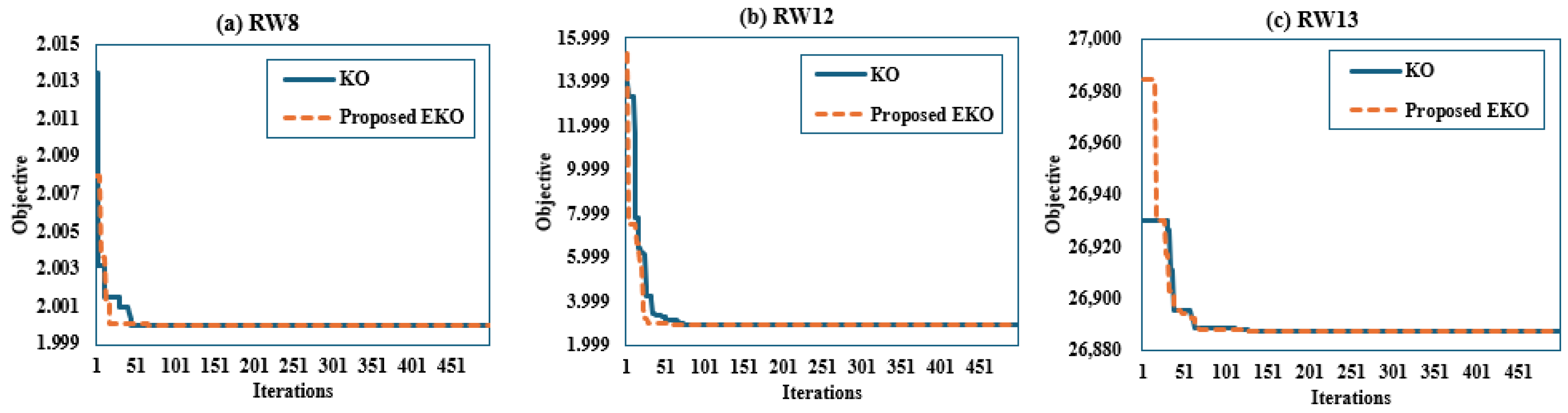
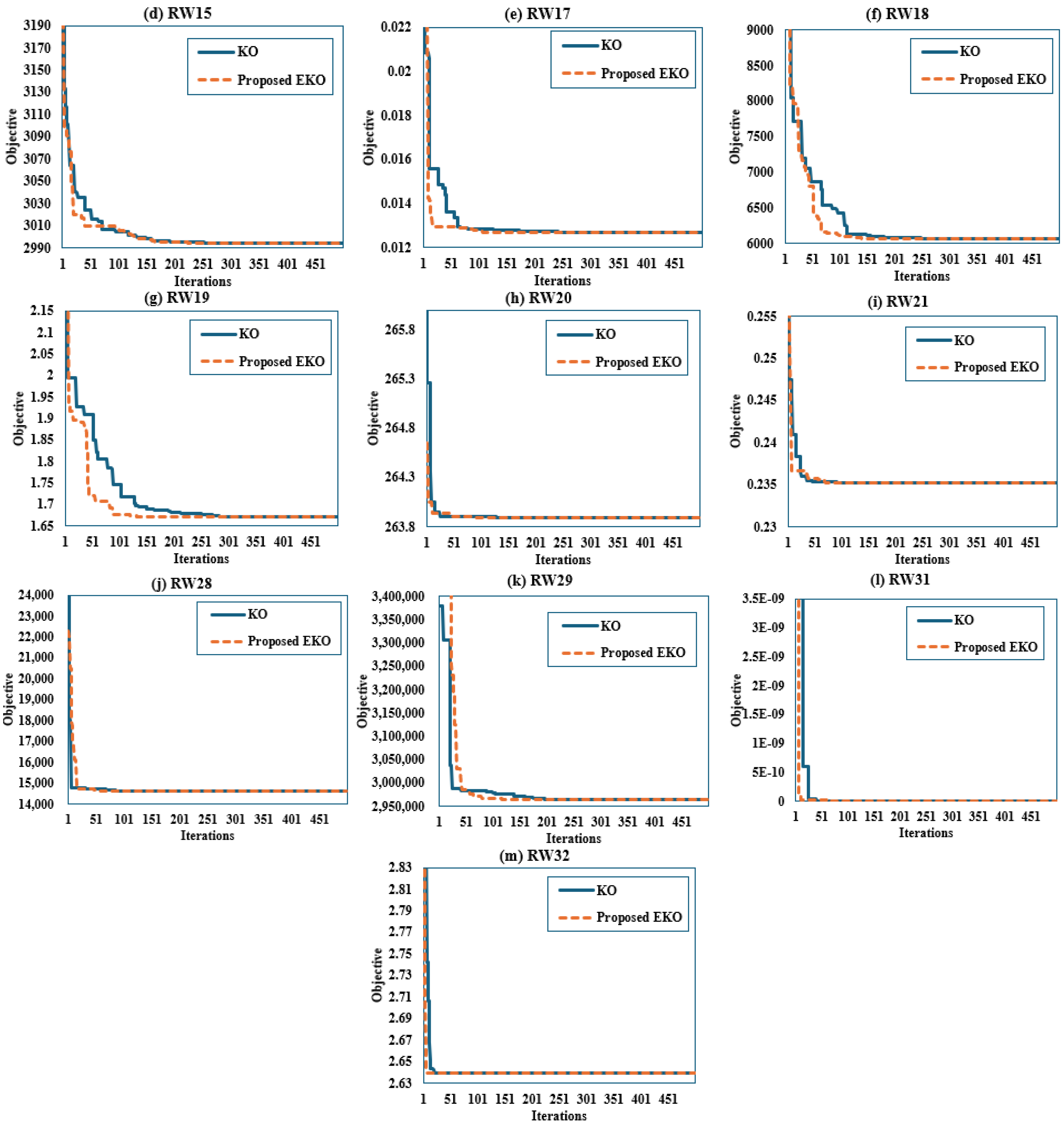
In the presented case studies, the firm penalty method was employed to manage the constraints. The population size was fixed at 200 for all 13 benchmarks, with a maximum of 500 iterations set for each case study. The key details regarding the benchmark functions and the inequality constraints employed in the investigation were considered [33] (their industrial data are displayed in Appendix A). They were process synthesis problems (RW8 and RW12), process design problem (RW13), speed reducer design (RW15), tension/compression spring design (RW17), pressure vessel design (RW18), welded beam design (RW19), three-bar truss design (RW20), multiple disk clutch brake design (RW21), rolling element bearing (RW28), gas transmission compressor design (RW29), gear train design (RW31), and Himmel Lau’s function (RW32).
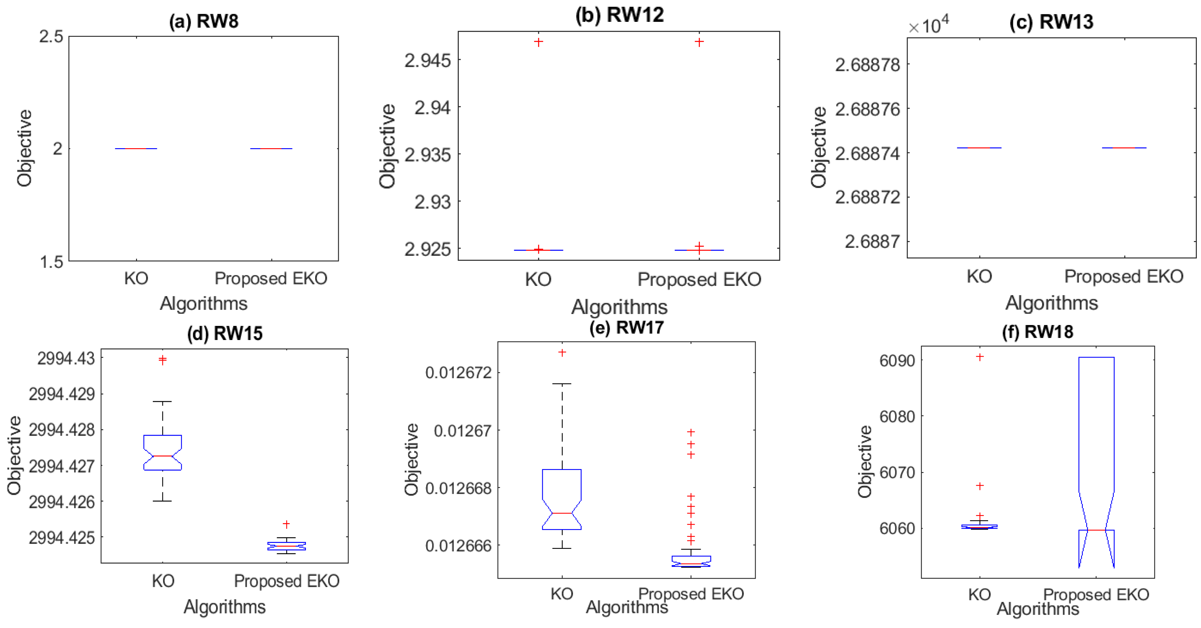
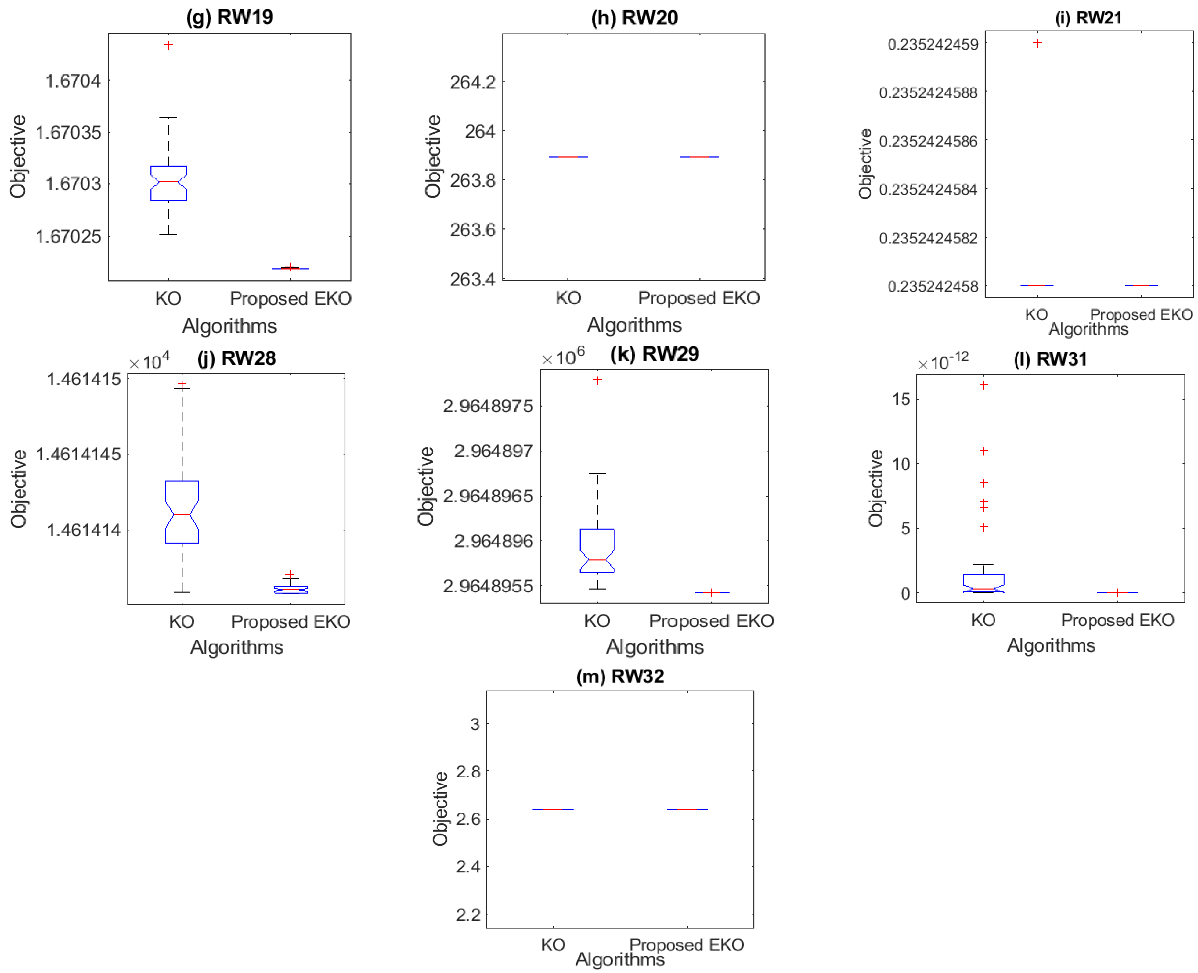
The proposed EKO and the standard KO methods were applied for fifty different runs and the resultant boxplots are shown in Figure 4 while the related average converging properties are depicted in Figure 5. The comparison reveals noteworthy observations:
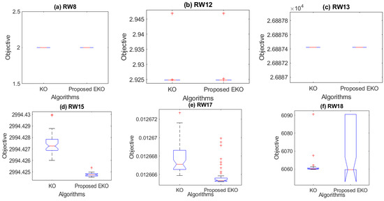
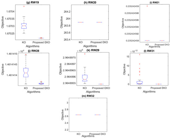
Figure 4.
Boxplots of the proposed EKO and KO for RW engineering problems.
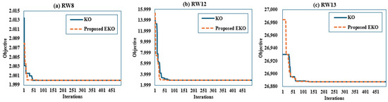
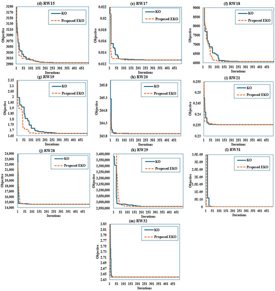
Figure 5.
Convergence curves of the proposed EKO and KO for RW engineering problems.
- The proposed EKO consistently achieved the lowest minimum objective in eleven RW problems, showcasing an impressive 84.61% outperformance ratio compared to the standard KO. Interestingly, both techniques exhibited similar performance in RW8 and RW32 problems.
- In terms of mean objective scores, the proposed EKO outperformed the standard KO in ten RW problems, with a notable 76.92% outperformance ratio. Conversely, the standard KO achieved lower scores in only two RW problems (RW12 and RW18) compared to the proposed EKO, while both techniques yielded comparable results in the RW32 problem.
- Analysis of the maximum objective scores indicates that the proposed EKO excelled in twelve RW problems, demonstrating a significant 92.3% outperformance ratio against the standard KO. Additionally, both methods yielded similar scores in the RW32 problem.
- Examination of the standard deviation in the attained objective scores reveals that the proposed EKO achieved the lowest values in ten RW problems, showcasing a substantial 76.92% outperformance ratio compared to the standard KO. Conversely, the standard KO attained smaller values in only two RW problems (RW12 and RW18) compared to the proposed EKO, while both techniques exhibited similar performance in RW32 problem.
4.1.2. Comparative Assessment against Other Techniques
The achieved outcomes were compared against other optimization solvers including WSO [34], DBO [35], MFO [36], LWSO [33], and FOX algorithms [37]. Table 2 compares the efficiency of the suggested EKO algorithm with other competing optimization methods for each of the 13 RW case studies. In this table, the symbols Min., Av., Med., Max., and STd indicate the best, average, median, worst, and the standard deviation of the obtained fitness scores for the fifty different runs implemented by the algorithms. Also, rank refers to the order of each algorithm, where the best performing one takes the first place in the order. The order is made based on the lowest values of the Min., Av., Med., Max,. and STd metrics. As shown, the average rank offers insights into the relative performance of algorithms across the evaluated criteria. A lower average rank signifies better performance. The proposed EKO demonstrates superiority with an average rank of 2.384615, indicating its effectiveness across the metrics considered. Therefore, the proposed EKO secures the top position with a final ranking of 1, highlighting its overall superiority among the evaluated algorithms. Assessing the average rank, notable improvements in the proposed EKO over each algorithm are highlighted. The proposed EKO demonstrates the most substantial enhancement, with a 59.74% improvement compared to FOX. Additionally, it achieves significant improvements of 38.0%, 35.417%, and 34.043% compared to DBO, MFO, and WSO, respectively. In comparison to the standard KO, the proposed EKO algorithm shows a noteworthy improvement of 26.19%. Lastly, it exhibits the lowest improvement of 22.5% compared to LWSO.
Table 2.
Statistical metrics for the RW engineering benchmarks under study.
4.2. Application on Multi-Area Power Systems with WTG
Three distinct controllers’ performances were examined while taking simultaneous step load variations in the thermal and wind regions into account. The power system discussed in Section 2 is modelled in this section under MATLAB SIMULINK, and relevant values are derived from [22]. Consequently, the following analysis is conducted on three distinct cases:
- Case 1: PI Controller;
- Case 2: PIDn Controller;
- Case 3: Proposed PI–(1+DD) Controller.
For this purpose, the proposed EKO algorithm and the standard KO algorithm were applied with comparative assessment against well-known efficient algorithms such as DE [38], SFO [39] and PSO [40,41]. The population size was fixed at 20 for all three cases, with a maximum of 100 iterations set for each case study and 20 separately running executions.
4.2.1. Case 1: PI Controller
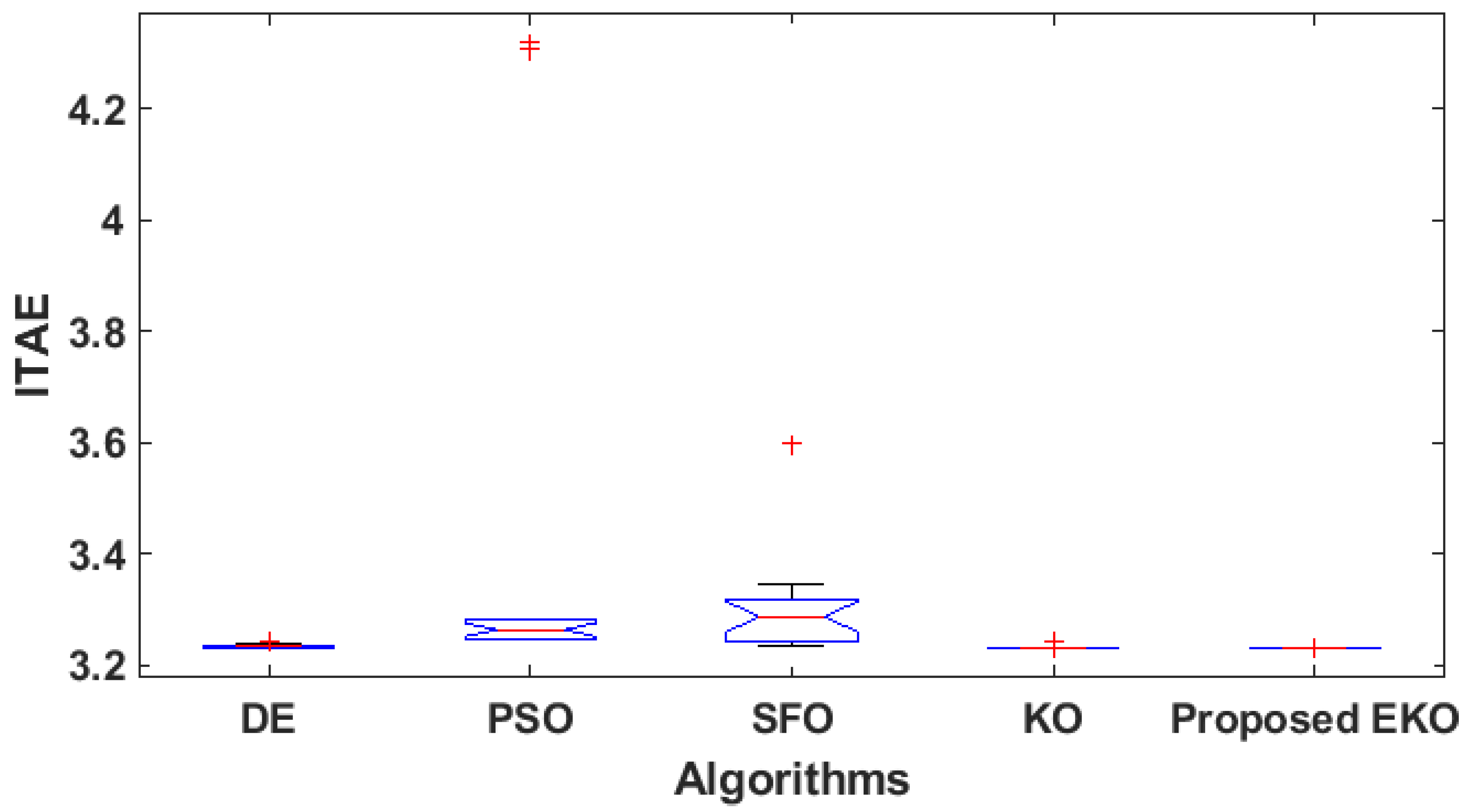
In this case, both areas were subjected to an additional 10% step load, and the controller was developed using the PI framework. Table 3 presents the gains (KP and KI) that were obtained by the suggested EKO, KO, PSO, DE, and SFO algorithms for each area. Comparing each algorithm against the proposed EKO, it is evident that the proposed EKO outperforms all other algorithms in terms of minimizing the ITAE. Notably, the ITAE value achieved by the EKO (3.232379096) is lower than that of DE (3.232596), PSO (3.247192601), SFO (3.234732), and KO (3.232469).
Table 3.
Optimized gains using DE, PSO, SFO, KO, and EKO for Case 1.
To estimate the improvement percentage of each algorithm compared to the proposed EKO, we can use the following formula:
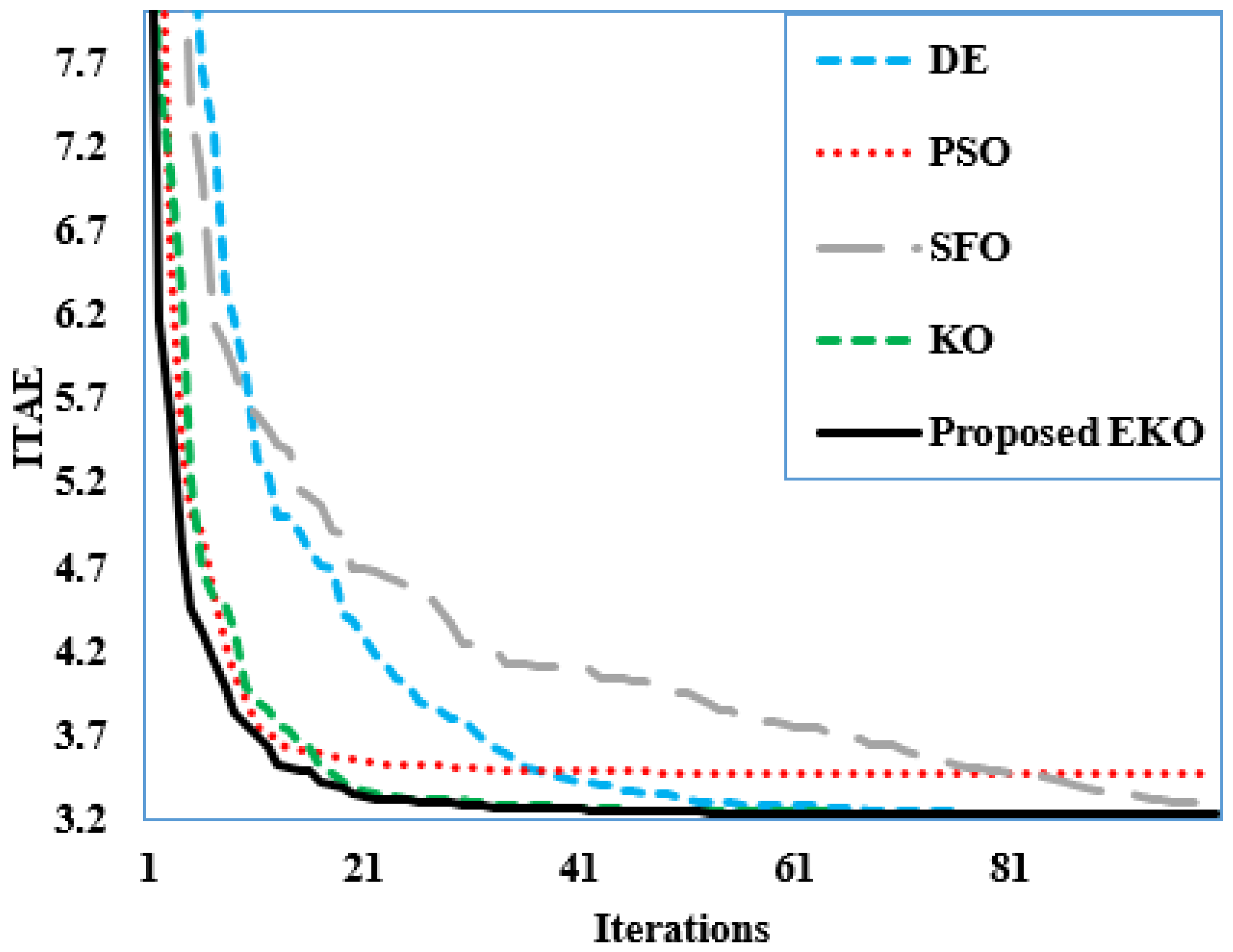
From Table 3, the EKO algorithm demonstrates the lowest ITAE score with 3.232379 while DE, PSO, SFO, and KO achieve ITAE counterparts of 3.232596, 3.247192601, 3.234732, and 3.232469, respectively. Also, the table illustrates the improvement percentages, showing how much better the proposed EKO performs compared to each algorithm in terms of minimizing ITAE. As shown, the EKO algorithm demonstrates a substantial improvement over PSO, of 0.456%, and small improvements over the DE, SFO, and KO algorithms of 0.0067%, 0.0727% and 0.0028%, respectively. Added to that, Figure 6 displays the boxplots of the DE, PSO, SFO, KO, and proposed EKO algorithms for this case, while Figure 7 shows the average converging characteristics of the DE, PSO, SFO, KO, and proposed EKO algorithms. Table 4 presents a comparative analysis of the efficiency of the proposed EKO algorithm against DE, PSO, SFO, and KO. The results reveal significant enhancements achieved by the proposed EKO in mean ITAE values, with improvements of 0.0639%, 6.8793%, 1.9309%, and 0.0213% compared to DE, PSO, SFO, and KO, respectively. Moreover, notable enhancements are observed in the worst ITAE values, where the proposed EKO achieves improvements of 0.2751%, 25.1534%, 10.1625%, and 0.2998% compared to DE, PSO, SFO, and KO, respectively. Finally, the proposed EKO declares great superiority in achieving the lowest standard deviation of 5.35385× 10⁻⁵, where DE, PSO, SFO, and KO correspondingly attain 0.00234, 0.4338, 0.08087 and 0.00217, respectively. These findings underscore the effectiveness of the proposed EKO algorithm in optimizing the PI controller’s performance across various evaluation metrics, highlighting its superiority over existing optimization methods.
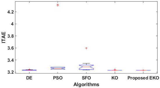
Figure 6.
Boxplots of the DE, PSO, SFO, KO, and proposed EKO for Case 1.
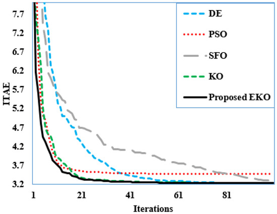
Figure 7.
Average converging characteristics of DE, PSO, SFO, KO, and proposed EKO for Case 1.
Table 4.
Statistical metrics for DE, PSO, SFO, KO, and proposed EKO for Case 1.
4.2.2. Case 2: PID Controller
In this case, the controller was developed using the PID framework while every zone required a 0.1 step increase in power. Table 5 shows the lowest ITAE values for the PID controller’s ideal settings when employing the suggested EKO, KO, PSO, DE, and SFO algorithms. Comparing each algorithm against the proposed EKO algorithm reveals that EKO significantly outperforms all other algorithms in terms of minimizing the ITAE. The ITAE metric emphasizes quick error correction by penalizing errors more heavily as time progresses. In this study, the EKO achieved an ITAE value of 0.238278, which is considerably lower than the values achieved by other algorithms: DE recorded an ITAE of 0.315377, PSO achieved 0.259712, SFO had 0.298104, and the original KO achieved 0.257969. Also, the EKO algorithm demonstrated substantial improvements over the other algorithms, ranging from approximately 7.63% to 24.44%. These results highlight the superior performance of EKO in efficiently handling and reducing errors over time, thereby ensuring a more stable and reliable control system. This improvement can be attributed to EKO’s advanced optimization capabilities, which enhance search efficiency and avoid premature convergence.
Table 5.
Optimized gains using DE, PSO, SFO, KO, and EKO for Case 2.
Added to that, Figure 8 displays the boxplots of the DE, PSO, SFO, KO, and proposed EKO for this case, while Figure 9 shows the average converging characteristics of the DE, PSO, SFO, KO, and proposed EKO. In this regard, Table 6 compares the efficiency of the suggested EKO algorithm with DE, PSO, SFO, and KO. As demonstrated, the proposed EKO algorithm achieves significant improvements in the mean ITAE values, exhibiting enhancements of 11.0806%, 26.3919%, 20.3443%, and 0.9371% compared to DE, PSO, SFO, and KO, respectively. Similarly, notable enhancements are observed in the median ITAE values, with the proposed EKO showing improvements of 12.1636%, 10.0203%, 16.4046%, and 7.0816% compared to DE, PSO, SFO, and KO, respectively. Additionally, substantial enhancements are evident in the worst ITAE values, with the proposed EKO achieving improvements of 2.0098%, 45.1480%, 44.7940%, and 3.0891% compared to DE, PSO, SFO, and KO, respectively. These results underscore the efficacy of the proposed EKO algorithm in optimizing the performance of the PID controller across various metrics, showcasing its superiority over existing optimization techniques.
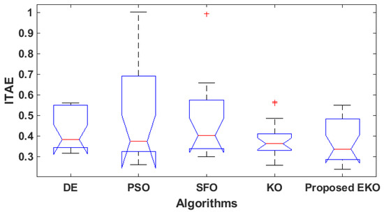
Figure 8.
Boxplots of the DE, PSO, SFO, KO, and proposed EKO for Case 2.
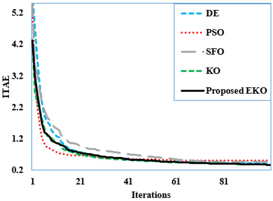
Figure 9.
Average converging characteristics of the DE, PSO, SFO, KO, and proposed EKO for Case 2.
Table 6.
Statistical metrics for DE, PSO, SFO, KO, and proposed EKO for Case 2.
Moreover, Figure 10, Figure 11 and Figure 12 display the change in the transfer power frequencies for the DE, PSO, SFO, KO, and proposed EKO algorithms for this case. The proposed EKO algorithm demonstrates significant improvements in system stability, as evidenced by its performance metrics compared to the other optimization techniques. In the case of frequency change in Area 1, as illustrated in Figure 10, the proposed EKO achieves the shortest settling time of 3.95 s, outperforming DE, PSO, SFO, and KO, which record settling times of 3.9851, 3.9973, 4.0023, and 9.6391 s, respectively. Moreover, the proposed EKO exhibits the smallest rise time of 0.00016 s, matching the performance of PSO, while KO, SFO, and DE achieve rise times of 0.0016, 0.0086, and 0.0238 s, respectively. Similarly, for the frequency change in Area 2 depicted in Figure 11, PSO, DE, and the proposed EKO achieve settling times of 2.76, 2.86, and 2.91 s, respectively, while SFO and KO require 3.5 and 4.19 s, respectively. Furthermore, in the case of transfer power change shown in Figure 12, the proposed EKO demonstrates the shortest settling time of 7.51 s, compared to DE, PSO, SFO, and KO, which record settling times of 9.5830, 8.0135, 9.6733, and 9.5585 s, respectively. These results highlight the superior performance and stability-enhancing capabilities of the proposed EKO algorithm, indicating its suitability for optimizing control strategies in dynamic power system environments.
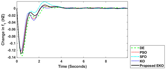
Figure 10.
Change in frequency (Area 1) regarding the DE, PSO, SFO, KO, and proposed EKO algorithms for Case 2.
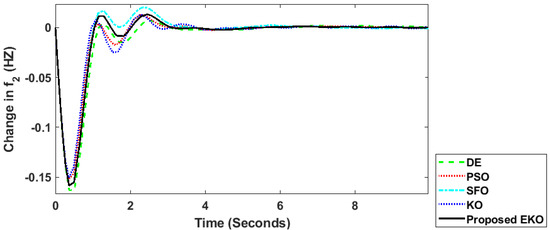
Figure 11.
Change in frequency (Area 2) regarding the DE, PSO, SFO, KO, and proposed EKO algorithms for Case 2.
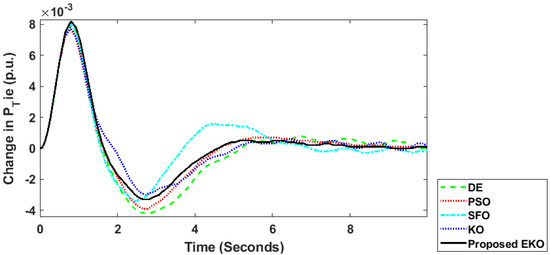
Figure 12.
Change in transfer power between areas regarding the DE, PSO, SFO, KO, and proposed EKO algorithms for Case 2.
4.2.3. Case 3: Proposed PI–(1+DD) Controller
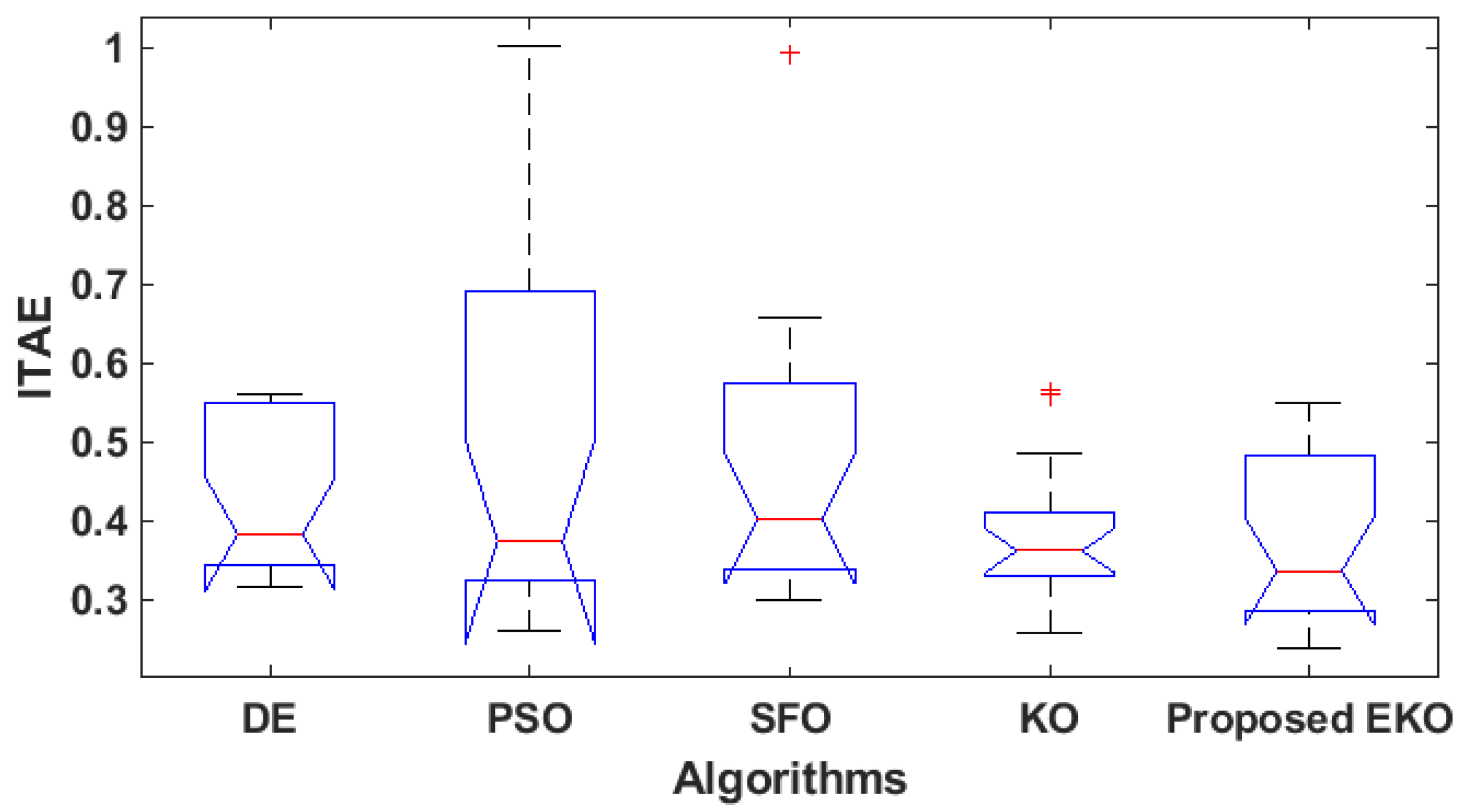
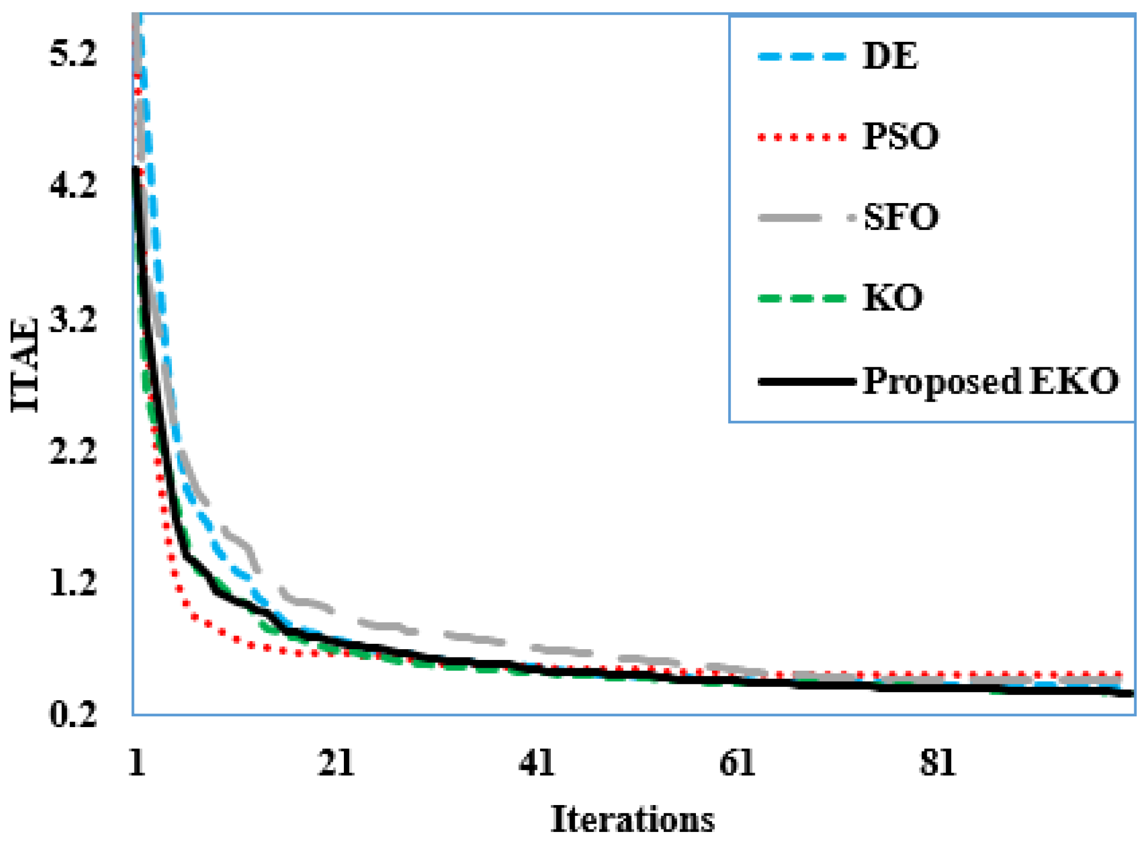
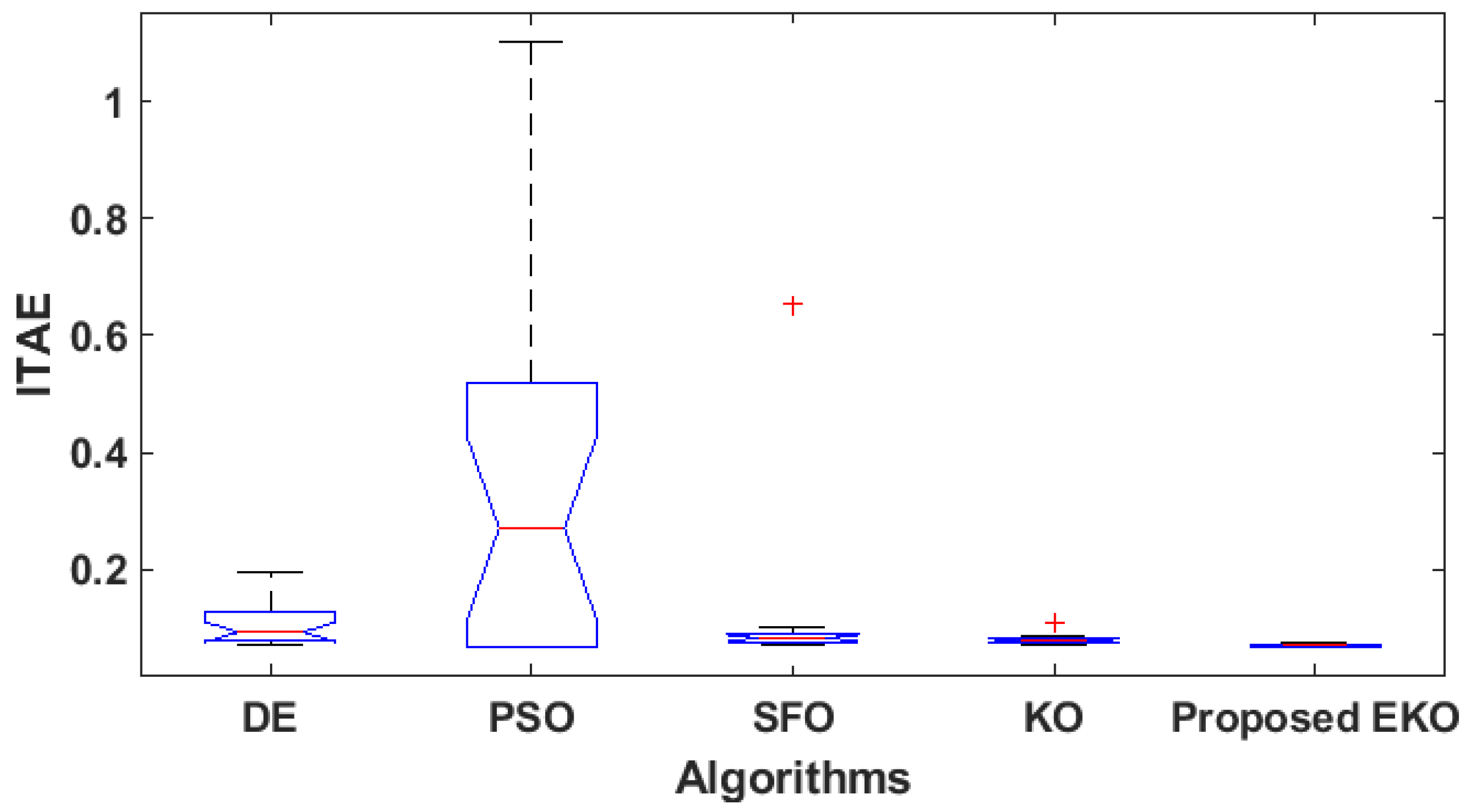
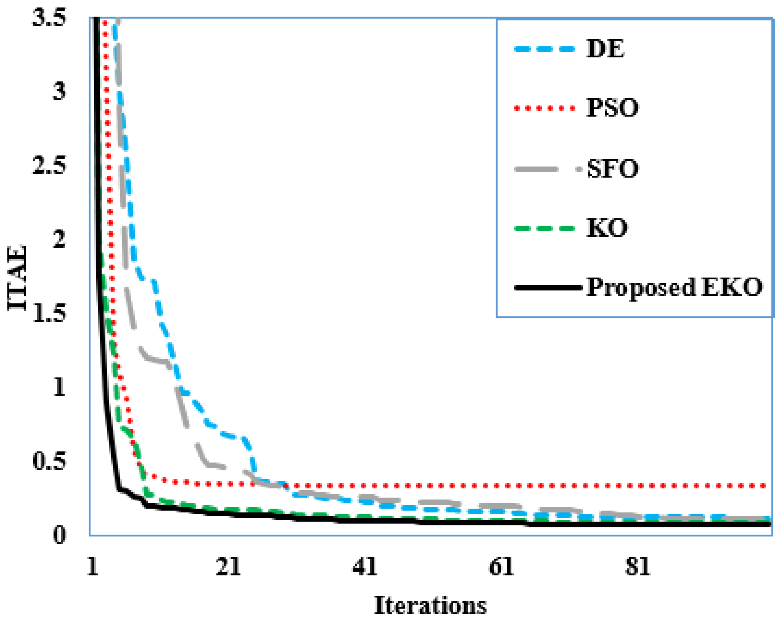
In this case, the controller was developed using the proposed PI–(1+DD) framework. Table 7 shows the lowest ITAE values for the proposed PI–(1+DD) controller settings when employing the suggested EKO, KO, PSO, DE, and SFO algorithms. Comparing each algorithm against the proposed EKO, it is evident that the proposed EKO outperforms all other algorithms in terms of minimizing the ITAE. Notably, the ITAE value achieved by the EKO (0.068234) is lower than that of DE (0.071969), PSO (0.068583), SFO (0.069858), and KO (0.069735). As shown, the EKO algorithm demonstrates substantial improvements over the DE, PSO, SFO, and KO algorithms of 5.1902%, 0.5095%, 2.3251%, and 2.1530%, respectively. In addition, Figure 13 displays the boxplots of the DE, PSO, SFO, KO, and proposed EKO algorithms for this case, while Figure 14 shows the average converging characteristics of the DE, PSO, SFO, KO and proposed EKO algorithms.
Table 7.
Optimized gains using DE, PSO, SFO, KO and EKO for Case 3.
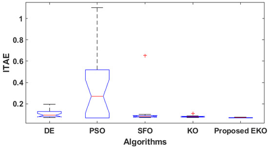
Figure 13.
Boxplots of the DE, PSO, SFO, KO and proposed EKO algorithms for Case 3.

Figure 14.
Converging characteristics of the DE, PSO, SFO, KO, and proposed EKO algorithms for Case 3.
In this regard, Table 8 compares the efficiency of the suggested EKO algorithm with the DE, PSO, SFO and KO algorithms. As demonstrated, the proposed EKO algorithm achieves significant improvements in the mean ITAE values, exhibiting enhancements of 37.1845%, 78.8091%, 36.8516%, and 12.2815% compared to DE, PSO, SFO, and KO, respectively. Similarly, notable enhancements are observed in the median ITAE values, with the proposed EKO showing improvements of 25.1049%, 74.2522%, 15.9631%, and 10.6539% compared to DE, PSO, SFO, and KO, respectively. Additionally, substantial enhancements are evident in the worst ITAE values, with the proposed EKO achieving improvements of 61.5404%, 93.2302%, 88.5823%, and 31.0667% compared to DE, PSO, SFO, and KO, respectively. These results underscore the efficacy of the proposed EKO algorithm in optimizing the performance of the proposed PI–(1+DD) controller across various metrics, showcasing its superiority over existing optimization techniques.
Table 8.
Statistical metrics for the DE, PSO, SFO, KO, and proposed EKO algorithms for Case 3.
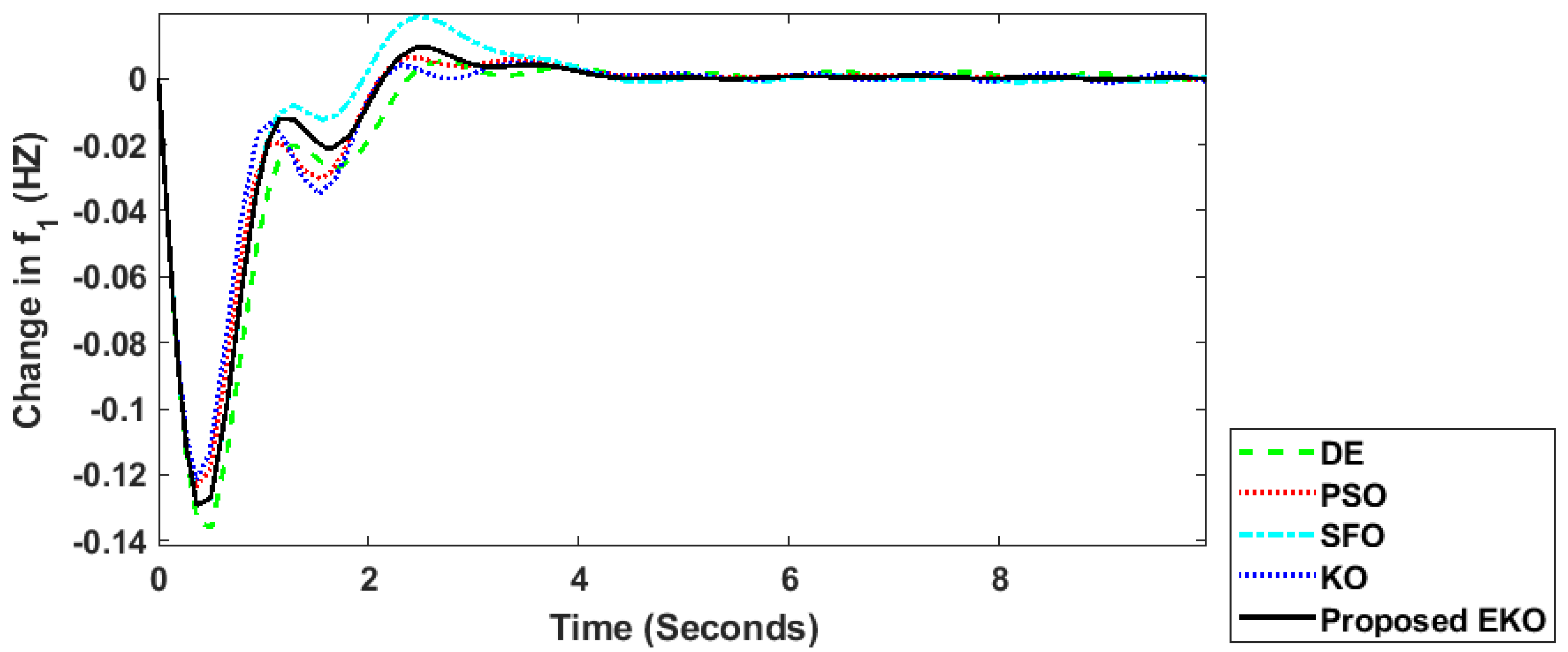
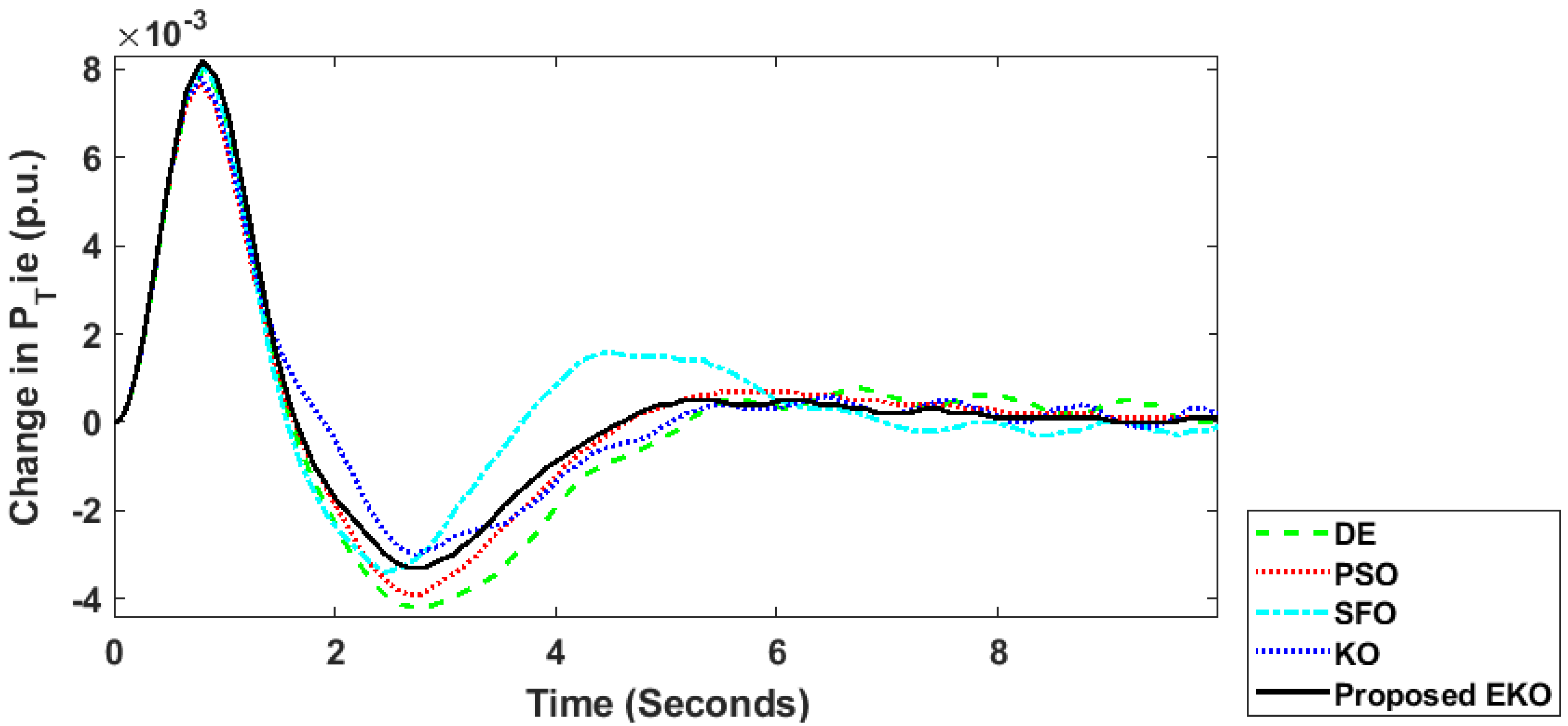
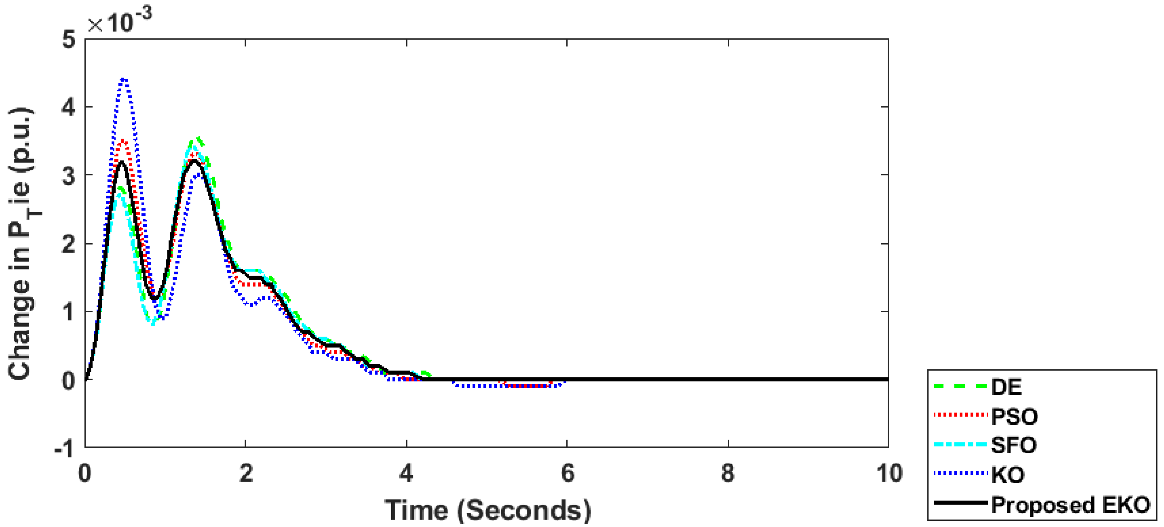
Moreover, Figure 15, Figure 16 and Figure 17 display the change in the transfer power frequencies of the DE, PSO, SFO, KO, and proposed EKO algorithms for this case. The proposed EKO algorithm demonstrates significant improvements in system stability, as evidenced by its performance metrics compared to other optimization techniques. Similarly, for the frequency change in Area 1 depicted in Figure 15, KO, DE, PSO, the proposed EKO algorithm, and SFO achieve comparable settling times of 2.94, 2.94, 2.95, 2.96, and 3 s, respectively. In the case of frequency change in Area 2, as illustrated in Figure 16, the proposed EKO algorithm achieves the shortest settling time of 2.148 s, outperforming DE, PSO, SFO, and KO, which record settling times of 2.2182, 2.2049, 2.1746, and 2.2893 s, respectively. Moreover, in the case of transfer power change shown in Figure 17, the proposed EKO algorithm demonstrates the shortest settling time of 4.097 s, compared to DE, PSO, SFO, and KO, which record settling times of 4.2785, 5.7654, 4.1196, and 5.8834 s, respectively.
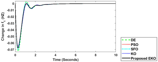
Figure 15.
Change in frequency (Area 1) regarding the DE, PSO, SFO, KO and proposed EKO algorithms for Case 3.
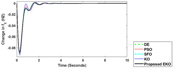
Figure 16.
Change in frequency (Area 2) regarding the DE, PSO, SFO, KO, and proposed EKO for Case 3.
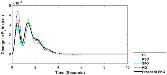
Figure 17.
Change in transfer power between areas regarding the DE, PSO, SFO, KO, and proposed EKO for Case 3.
5. Conclusions
In this study, an EKO algorithm is presented, incorporating additional fractional-order components. The performance of the proposed EKO algorithm was evaluated through simulations of RW engineering design problems and its application in optimizing control strategies for multi-area power systems with WTG. Firstly, the simulation results demonstrate that the proposed EKO algorithm consistently outperformed the standard KO method across various RW engineering design problems, achieving lower minimum, mean, and maximum objective scores, as well as smaller standard deviations. Comparative assessments against other optimization techniques further confirmed the superiority of the proposed EKO, showcasing substantial improvements in efficiency and effectiveness across multiple evaluation metrics. Secondly, in the application to multi-area power systems with WTG, the proposed EKO algorithm demonstrated remarkable performance in optimizing the PI, PID, and proposed PI–(1+DD) controllers. It consistently achieved lower ITAE values compared to other algorithms, indicating superior frequency regulation capabilities. Moreover, the proposed EKO exhibited enhanced stability and faster settling times in response to frequency and transfer power changes, highlighting its suitability for dynamic power system environments. The EKO algorithm proposed in this paper performs excellently in load frequency control, particularly in addressing frequency stability issues in multi-area power systems with wind power integration. The experimental results show that compared to the traditional KO and other algorithms, the EKO algorithm significantly improves system frequency stability. Future work will include further optimization of the algorithm parameters and validation of its effectiveness in larger-scale power systems. Also, it can be extended to improve distribution system performance with active smart grid functions.
Author Contributions
Conceptualization, M.H.A. and A.M.S.; Methodology, M.H.A., A.M.S., G.M. and A.A.E.-F.; Software, M.H.A., A.M.S. and A.A.E.-F.; Validation, M.H.A., S.Z.A., A.S.A. and A.M.S.; Formal analysis, M.H.A., A.M.S., G.M. and A.A.E.-F.; Resources, A.S.A.; Data curation, S.Z.A. and G.M.; Writing—original draft, M.H.A., S.Z.A., A.M.S. and A.A.E.-F.; Writing—review & editing, A.S.A., A.M.S., G.M. and A.A.E.-F.; Visualization, A.S.A.; Supervision, S.Z.A.; Project administration, M.H.A.; Funding acquisition, M.H.A. All authors have read and agreed to the published version of the manuscript.
Funding
The authors extend their appreciation to Prince Sattam bin Abdulaziz University for funding this research work through the project number (PSAU/2023/01/9076).
Data Availability Statement
The original contributions presented in the study are included in the article/supplementary material, further inquiries can be directed to the corresponding authors.
Conflicts of Interest
The authors declare no conflict of interest.
Abbreviations
| CEC 2020 | Congress on Evolutionary Computation 2020 |
| DBO | Dung Beetle optimizer |
| DFIG | Doubly fed induction generator |
| EKO | Enhanced Kepler Optimization |
| GL | Grunwald–Letnikov |
| I | Integral |
| ITAE | Integral time-multiplied absolute value of the error |
| KO | Kepler Optimization |
| LEA | Local Escaping Approach |
| LFC | load frequency control |
| LWSO | Leader White Shark Optimization |
| MFO | Moth-Flame Optimizer |
| PI | Proportional-integral |
| PID | Proportional-integral–derivative |
| PI-(1+DD) | Proportional-Integral-First-Order Double Derivative |
| PSO | Particle Swarm Optimization |
| RESs | Renewable energy sources |
| RW | Real-world |
| SFO | Sunflower Optimizer |
| WSO | White Shark Optimization |
| WT | Wind turbine |
Appendix A
Table A1 showcases the RW optimization engineering benchmark cases featured in the CEC 2020 competition.
Table A1.
RW benchmarks included in the CEC 2020.
Table A1.
RW benchmarks included in the CEC 2020.
| Function | Case Study Problem | Decision Variables | Constraints | Global Optima |
|---|---|---|---|---|
| RW8 | Process synthesis | 2.0 | 2.0 | 2.0 |
| RW12 | Process synthesis | 7.0 | 9.0 | 2.92 |
| RW13 | Process design | 5.0 | 3.0 | 26,900 |
| RW15 | Weight minimization of a speed reducer | 7.0 | 11.0 | 2990.0 |
| RW17 | Tension/compression spring design (Case 1) | 3.0 | 3.0 | 0.0127 |
| RW18 | Pressure vessel design | 4.0 | 4.0 | 5890.0 |
| RW19 | Welded beam design | 4.0 | 5.0 | 1.67 |
| RW20 | Three-bar truss design | 2.0 | 3.0 | 264.0 |
| RW21 | Multiple disk clutch brake design | 5.0 | 7.0 | 0.0235 |
| RW28 | Rolling element bearing | 10.0 | 9.0 | 14,600.0 |
| RW29 | Gas transmission compressor design | 4.0 | 1.0 | 2,960,000.0 |
| RW31 | Gear train design | 4.0 | 1.0 | 0.0 |
| RW32 | Himmel Lau’s function | 5.0 | 6.0 | −30,700.0 |
References
- Shayeghi, H.; Shayanfar, H.; Jalili, A. Load frequency control strategies: A state-of-the-art survey for the researcher. Energy Convers. Manag. 2009, 50, 344–353. [Google Scholar] [CrossRef]
- Agathokleous, C.; Ehnberg, J. A Quantitative Study on the Requirement for Additional Inertia in the European Power System until 2050 and the Potential Role of Wind Power. Energies 2020, 13, 2309. [Google Scholar] [CrossRef]
- Nguyen, H.T.; Yang, G.; Nielsen, A.H.; Jensen, P.H. Combination of Synchronous Condenser and Synthetic Inertia for Frequency Stability Enhancement in Low-Inertia Systems. IEEE Trans. Sustain. Energy 2018, 10, 997–1005. [Google Scholar] [CrossRef]
- Li, Q.; Ren, B.; Tang, W.; Wang, D.; Wang, C.; Lv, Z. Analyzing the inertia of power grid systems comprising diverse conventional and renewable energy sources. Energy Rep. 2022, 8, 15095–15105. [Google Scholar] [CrossRef]
- Rapizza, M.R.; Canevese, S.M. Fast frequency regulation and synthetic inertia in a power system with high penetration of renewable energy sources: Optimal design of the required quantities. Sustain. Energy Grids Netw. 2020, 24, 100407. [Google Scholar] [CrossRef]
- Liu, X.; Qiao, S.; Liu, Z. A Survey on Load Frequency Control of Multi-Area Power Systems: Recent Challenges and Strategies. Energies 2023, 16, 2323. [Google Scholar] [CrossRef]
- Maurya, A.K.; Khan, H.; Ahuja, H. Stability Control of Two-Area of Power System Using Integrator, Proportional Integral and Proportional Integral Derivative Controllers. In Proceedings of the 2023 International Conference on Artificial Intelligence and Smart Communication (AISC), Greater Noida, India, 27–29 January 2023; pp. 273–278. [Google Scholar]
- Lu, K.; Zhou, W.; Zeng, G.; Zheng, Y. Constrained population extremal optimization-based robust load frequency control of multi-area interconnected power system. Int. J. Electr. Power Energy Syst. 2018, 105, 249–271. [Google Scholar] [CrossRef]
- Arora, K.; Kumar, A.; Kamboj, V.K.; Prashar, D.; Jha, S.; Shrestha, B.; Joshi, G.P. Optimization Methodologies and Testing on Standard Benchmark Functions of Load Frequency Control for Interconnected Multi Area Power System in Smart Grids. Mathematics 2020, 8, 980. [Google Scholar] [CrossRef]
- Dahab, Y.A.; Abubakr, H.; Mohamed, T.H. Adaptive Load Frequency Control of Power Systems Using Electro-Search Optimization Supported by the Balloon Effect. IEEE Access 2020, 8, 7408–7422. [Google Scholar] [CrossRef]
- Guha, D.; Roy, P.K.; Banerjee, S. Maiden application of SSA-optimised CC-TID controller for load frequency control of power systems. IET Gener. Transm. Distrib. 2019, 13, 1110–1120. [Google Scholar] [CrossRef]
- Mary, V.B.; Narmadha, T.V. Optimization of Integrated Hybrid Systems Using Model Predictive Controller. Electr. Power Components Syst. 2023, 52, 82–98. [Google Scholar] [CrossRef]
- Riquelme, E.; Chavez, H.; Barbosa, K.A. RoCoF-Minimizing H₂ Norm Control Strategy for Multi-Wind Turbine Synthetic Inertia. IEEE Access 2022, 10, 18268–18278. [Google Scholar] [CrossRef]
- Yedrzejewski, N.; Giusto, A. Potential impact of wind-based Synthetic Inertia on the Frequency Response of the Argentine-Uruguayan Interconnected Power Systems. In Proceedings of the 2022 IEEE PES Innovative Smart Grid Technologies—Asia (ISGT Asia), Singapore, 1–5 November 2022; pp. 505–509. [Google Scholar]
- Roy, N.K.; Islam, S.; Podder, A.K.; Roy, T.K.; Muyeen, S.M. Virtual Inertia Support in Power Systems for High Penetration of Renewables—Overview of Categorization, Comparison, and Evaluation of Control Techniques. IEEE Access 2022, 10, 129190–129216. [Google Scholar] [CrossRef]
- Raj, T.D.; Kumar, C.; Kotsampopoulos, P.; Fayek, H.H. Load Frequency Control in Two-Area Multi-Source Power System Using Bald Eagle-Sparrow Search Optimization Tuned PID Controller. Energies 2023, 16, 2014. [Google Scholar] [CrossRef]
- Adu, J.A.; Tossani, F.; Pontecorvo, T.; Ilea, V.; Vicario, A.; Conte, F.; D’Agostino, F. Coordinated Inertial Response Provision by Wind Turbine Generators: Effect on Power System Small-Signal Stability of the Sicilian Network. In Proceedings of the 2022 IEEE International Conference on Environment and Electrical Engineering and 2022 IEEE Industrial and Commercial Power Systems Europe (EEEIC/I&CPS Europe), Prague, Czech Republic, 28 June–1 July 2022; pp. 1–6. [Google Scholar]
- Abid, S.; El-Rifaie, A.M.; Elshahed, M.; Ginidi, A.R.; Shaheen, A.M.; Moustafa, G.; Tolba, M.A. Development of Slime Mold Optimizer with Application for Tuning Cascaded PD-PI Controller to Enhance Frequency Stability in Power Systems. Mathematics 2023, 11, 1796. [Google Scholar] [CrossRef]
- Ibrahim, N.M.A.; Talaat, H.E.A.; Shaheen, A.M.; Hemade, B.A. Optimization of Power System Stabilizers Using Proportional-Integral-Derivative Controller-Based Antlion Algorithm: Experimental Validation via Electronics Environment. Sustainability 2023, 15, 8966. [Google Scholar] [CrossRef]
- Arora, K.; Kumar, A.; Kamboj, V.K.; Prashar, D.; Shrestha, B.; Joshi, G.P. Impact of Renewable Energy Sources into Multi Area Multi-Source Load Frequency Control of Interrelated Power System. Mathematics 2021, 9, 186. [Google Scholar] [CrossRef]
- Fan, W.; Hu, Z.; Veerasamy, V. PSO-Based Model Predictive Control for Load Frequency Regulation with Wind Turbines. Energies 2022, 15, 8219. [Google Scholar] [CrossRef]
- El-Ela, A.A.A.; El-Sehiemy, R.A.; Shaheen, A.M.; Diab, A.E.-G. Design of cascaded controller based on coyote optimizer for load frequency control in multi-area power systems with renewable sources. Control Eng. Pr. 2022, 121, 105058. [Google Scholar] [CrossRef]
- Sun, J.; Chen, M.; Kong, L.; Hu, Z.; Veerasamy, V. Regional Load Frequency Control of BP-PI Wind Power Generation Based on Particle Swarm Optimization. Energies 2023, 16, 2015. [Google Scholar] [CrossRef]
- Ali, G.; Aly, H.; Little, T. Automatic Generation Control of a Multi-Area Hybrid Renewable Energy System Using a Proposed Novel GA-Fuzzy Logic Self-Tuning PID Controller. Energies 2024, 17, 2000. [Google Scholar] [CrossRef]
- Abdel-Basset, M.; Mohamed, R.; Azeem, S.A.A.; Jameel, M.; Abouhawwash, M. Kepler optimization algorithm: A new metaheuristic algorithm inspired by Kepler’s laws of planetary motion. Knowl.-Based Syst. 2023, 268, 110454. [Google Scholar] [CrossRef]
- Hakmi, S.H.; Shaheen, A.M.; Alnami, H.; Moustafa, G.; Ginidi, A. Kepler Algorithm for Large-Scale Systems of Economic Dispatch with Heat Optimization. Biomimetics 2023, 8, 608. [Google Scholar] [CrossRef] [PubMed]
- Hasanien, H.M. Whale optimisation algorithm for automatic generation control of interconnected modern power systems including renewable energy sources. IET Gener. Transm. Distrib. 2017, 12, 607–614. [Google Scholar] [CrossRef]
- El-Sehiemy, R.; Shaheen, A.; Ginidi, A.; Al-Gahtani, S.F. Proportional-Integral-Derivative Controller Based-Artificial Rabbits Algorithm for Load Frequency Control in Multi-Area Power Systems. Fractal Fract. 2023, 7, 97. [Google Scholar] [CrossRef]
- Can, O.; Ozturk, A.; Eroğlu, H.; Kotb, H. A Novel Grey Wolf Optimizer Based Load Frequency Controller for Renewable Energy Sources Integrated Thermal Power Systems. Electr. Power Compon. Syst. 2021, 49, 1248–1259. [Google Scholar] [CrossRef]
- Moustafa, G.; Elshahed, M.; Ginidi, A.R.; Shaheen, A.M.; Mansour, H.S.E. A Gradient-Based Optimizer with a Crossover Operator for Distribution Static VAR Compensator (D-SVC) Sizing and Placement in Electrical Systems. Mathematics 2023, 11, 1077. [Google Scholar] [CrossRef]
- Podlubny, I. Fractional Differential Equations: An Introduction to Fractional Derivatives, Fractional Differential Equations, to Methods of Their Solution and Some of Their Applications; Elsevier: Amsterdam, The Netherlands, 1999; Volume 198. [Google Scholar]
- Kumar, A.; Wu, G.; Ali, M.Z.; Mallipeddi, R.; Suganthan, P.N.; Das, S. A test-suite of non-convex constrained optimization problems from the real-world and some baseline results. Swarm Evol. Comput. 2020, 56, 100693. [Google Scholar] [CrossRef]
- Hassan, M.H.; Kamel, S.; Selim, A.; Shaheen, A.; Yu, J.; El-Sehiemy, R. Efficient economic operation based on load dispatch of power systems using a leader white shark optimization algorithm. Neural Comput. Appl. 2024, 1–23. [Google Scholar] [CrossRef]
- Braik, M.; Hammouri, A.; Atwan, J.; Al-Betar, M.A.; Awadallah, M.A. White Shark Optimizer: A novel bio-inspired meta-heuristic algorithm for global optimization problems. Knowl.-Based Syst. 2022, 243, 108457. [Google Scholar] [CrossRef]
- Xue, J.; Shen, B. Dung beetle optimizer: A new meta-heuristic algorithm for global optimization. J. Supercomput. 2022, 79, 7305–7336. [Google Scholar] [CrossRef]
- Mirjalili, S. Moth-flame optimization algorithm: A novel nature-inspired heuristic paradigm. Knowl.-Based Syst. 2015, 89, 228–249. [Google Scholar] [CrossRef]
- Mohammed, H.; Rashid, T. FOX: A FOX-inspired optimization algorithm. Appl. Intell. 2022, 53, 1030–1050. [Google Scholar] [CrossRef]
- Ahmad, M.F.; Isa, N.A.M.; Lim, W.H.; Ang, K.M. Differential evolution: A recent review based on state-of-the-art works. Alex. Eng. J. 2022, 61, 3831–3872. [Google Scholar] [CrossRef]
- Shaheen, A.M.; Elattar, E.E.; El-Sehiemy, R.A.; Elsayed, A.M. An Improved Sunflower Optimization Algorithm-Based Monte Carlo Simulation for Efficiency Improvement of Radial Distribution Systems Considering Wind Power Uncertainty. IEEE Access 2020, 9, 2332–2344. [Google Scholar] [CrossRef]
- Kennedy, J.; Eberhart, R. Particle Swarm Optimization. In Proceedings of the IEEE International Conference on Neural Networks, Perth, WA, Australia, 27 November–1 December 1995. [Google Scholar]
- Wang, D.; Tan, D.; Liu, L. Particle swarm optimization algorithm: An overview. Soft Comput. 2018, 22, 387–408. [Google Scholar] [CrossRef]


Disclaimer/Publisher’s Note: The statements, opinions and data contained in all publications are solely those of the individual author(s) and contributor(s) and not of MDPI and/or the editor(s). MDPI and/or the editor(s) disclaim responsibility for any injury to people or property resulting from any ideas, methods, instructions or products referred to in the content. |
© 2024 by the authors. Licensee MDPI, Basel, Switzerland. This article is an open access article distributed under the terms and conditions of the Creative Commons Attribution (CC BY) license (https://creativecommons.org/licenses/by/4.0/).