Novel Controller Design for Finite-Time Synchronization of Fractional-Order Nonidentical Complex Dynamical Networks under Uncertain Parameters

Abstract

The synchronization of complex networks, as an important and captivating dynamic phenomenon, has been investigated across diverse domains ranging from social activities to ecosystems and power systems. Furthermore, the synchronization of networks proves instrumental in solving engineering quandaries, such as cryptography and image encryption. And finite-time synchronization (FTS) controls exhibit substantial resistance to interference, accelerating network convergence speed and heightening control efficiency. In this paper, finite-time synchronization (FTS) is investigated for a class of fractional-order nonidentical complex networks under uncertain parameters (FONCNUPs). Firstly, some new FTS criteria for FONCNUPs are proposed based on Lyapunov theory and fractional calculus theory. Then, the new controller is designed based on inequality theory. Compared to the general controller, it controls all nodes and adds additional control to some of them. When compared to other controllers, it has lower control costs and higher efficiency. Finally, a numerical example is presented to validate the effectiveness and rationality of the obtained results.

1. Introduction

Nowadays, complex networks are almost everywhere, and the study of complex networks has wide applications in various disciplines. For example, in sociology, it includes human relationships [1], information dissemination [2], collective behavior [3], etc. In biology, it includes the structure and function of biological systems [4,5]. In physics, it involves the reliability and stability of power systems [6], transportation networks [7], etc. Therefore, complex networks have attracted a large number of researchers from many fields.

Fractional calculus is an important branch of calculus. It is a mathematical concept that lies between integer-order differentiation and integration. In traditional integer-order calculus, the order of differentiation can only be a positive integer. However, in fractional calculus, the order can be any real or complex number, including decimals and fractions [8]. Fractional derivatives provide scientists with a new mathematical tool for solving problems with non-local characteristics and complex dynamical behavior. They can be used to describe phenomena with non-locality, such as long-term memory and non-stationary processes [9]. Fractional calculus has wide applications in various scientific fields, including chemistry, biology, and engineering [10,11,12]. Additionally, the study of fractional calculus is of great significance in uncovering many phenomena in nature, such as diffusion processes [13], circuits [14], and chaotic systems [15]. Therefore, fractional calculus has a broad and important prospect of applications in scientific research and engineering.

With the utilization of fractional calculus, researchers have commenced applying it to the realm of complex networks. An extension of traditional complex networks, fractional-order complex networks (FOCNs) integrate fractional derivatives and fractional differential equations to depict the dynamic behavior within networks. FOCNs prove more adept in capturing the complexity of real-world complex systems, including secure communications [16], mathematical biology [17], heat conduction [18], and hydrodynamics [19]. Relative to traditional complex networks, FOCNs excel in illustrating features, such as long-range dependence, non-stationarity, and network evolution. Nonlinear and non-local behavioral patterns persist in numerous complex systems, such as the brain and financial markets. Traditional integer-order calculus falls short in accurately characterizing these behaviors. Consequently, the study of FOCNs offers partial compensation for the limitations of integer-order models. Stemming from the investigation of real system behavior and advances in computational science, FOCNs have emerged as a thriving field of research within the domain of complex networks.

Nevertheless, real networks typically exhibit high nonidenticality, whereby the roles of distinct nodes and paths in the network evolution process deviate significantly. Consequently, nonidentical complex networks embrace heightened complexity and realism when compared to identical complex networks [20]. Within fractional-order nonidentical complex dynamic networks, the presence of parameter uncertainty renders network synchronization a formidable challenge. In such networks, both the connections between network nodes and dynamic behaviors of nodes fall under the influence of uncertain parameters [21]. Consequently, achieving synchronization necessitates consideration of these uncertain parameters as well.

Synchronization, as an important and captivating dynamic phenomenon, has been investigated across diverse domains ranging from social activities to ecosystems and power systems. Furthermore, synchronization proves instrumental in solving engineering quandaries, such as cryptography [22] and image encryption [23]. Extensive research has been dedicated to synchronization, encompassing phenomena like asymptotic synchronization [24], quasi synchronization [25], exponential synchronization, and others [26,27]. Depending on the desired synchronization time frame, synchronization can be categorized into infinite-time synchronization and FTS. Traditional approaches primarily focus on the behavior of error systems over an infinite-time interval. However, practical applications occasionally necessitate the attainment of synchronization within a finite convergence time. In comparison to infinite-time synchronization, FTS offers optimal convergence time, enhanced robustness, and superior interference attenuation performance. Additionally, FTS controls exhibit substantial resistance to interference, accelerating network convergence speed and heightening control efficiency [28,29]. Such traits have garnered considerable attention in practical applications, including transportation.

In the literature [30], Li proposed a new lemma based on fractional calculus theory to study the FTS problem, and a new feedback controller was designed based on the new lemma. In [31], Xiao established FTS conditions based on Lyapunov techniques and fractional calculus theory and designed different types of controllers according to the characteristics of neural networks to achieve FTS. In [32], Li utilized the fundamental theory of fractional calculus and Lyapunov theory to establish the fractional-order finite-time convergence principle. They also designed two novel adaptive nonlinear controllers and discontinuous nonlinear controllers to solve the complete synchronization and FTS problems of fractional-order fuzzy neural networks. In [33], Li designed quaternion feedback controllers and quaternion adaptive controllers to solve the robust FTS problem of the uncertain fractional-order quaternion neural networks. In [34], Xu combined the Lyapunov method with graph theory and established FTS criteria for fractional-order multi-weight complex dynamic networks using feedback control and adaptive control. In [35], using Lyapunov theory, differential inclusion theory, and fractional calculus theory, the FTS conditions and upper bounds of stable time for fractional-order memory complex-valued BAM neural networks were obtained. In [36], by using the Young inequality and the fractional derivative rule of composite functions, a new finite-time convergence principle related to time delays was derived. However, in previous studies, few researchers have simultaneously considered the FTS problem of fractional-order nonidentical complex networks under uncertain parameters. There is a lack of relevant research, and our research will enrich the existing research conclusions. So, it is important to investigate the FTS of FONCNUPs.

Motivated by the above discussions, we will study the FTS of FONCNUPs. The main contributions are as follows:

(1)

A new criterion for FOCNUP synchronization is proposed using fractional-order theory and inequality theory.

(2)

A new controller is designed to achieve the FTS of FOCNUPs.

(3)

Two general controllers are proposed and compared with the new controller proposed, and corresponding numerical simulations are performed to highlight the advantages of our proposed new controller.

The following passages present the remaining sections of this paper: Section 2 is the preliminaries. Some sufficient conditions for the FTS of FOCNUPs are given in Section 3. The rationality of the acquired results are verified by two numerical examples in Section 4. Ultimately, Section 5 shows the conclusion of this paper.

Notations: ${\mathbb{R}}^n$ represents the n-dimensional Euclidean space. ${\mathbb{R}}^{n\times n}$ denotes $n\times n$ matrices in the real field. $N^{\top }$ represents the transpose matrix of N. $\alpha$ is the derivative order. For any $e=(e_1,e_2,\cdots ,e_n)\in {\mathbb{R}}^n,$ $\parallel e\parallel ={\sum }_{i=1}^n|e_i|$ is the Euclidean norm. $C^m([t,+\infty ),\mathbb{R})$ represent the space consisting of m-order continuous differentiable functions from $[t,+\infty )$ into $\mathbb{R}$.

2. Preliminaries

Definition 1

([8]). The α-order fractional integral of function $\psi (t)$ is defined as

$$\begin{array}{c}\hfill I_t^{\alpha }\psi (t)=\frac{1}{\Gamma (\alpha )}{\int }_{t_0}^t{(t-s)}^{\alpha -1}\psi (s)ds,\alpha >0,\end{array}$$

(1)

where $t_0$ is the initial time, $t\ge t_0$, and $\Gamma (·)$ is the Gamma function.

Definition 2

([8]). The α-order Caputo fractional derivative of $\psi (t)$ is defined as

$$\begin{array}{c}\hfill { }_{t_0}^C{D}_t^{\alpha }\psi (t)=\frac{1}{\Gamma (\eta -\alpha )}{\int }_{t_0}^t{(t-\vartheta )}^{\eta -\alpha -1}\psi {(t)}^{(\eta )}(\vartheta )d\vartheta ,\end{array}$$

(2)

where $\eta -1<\alpha <\eta$, $\eta \in {\mathbb{Z}}^{+}$. When $0<\alpha <1,$

$$\begin{array}{c}\hfill { }_{t_0}^C{D}_t^{\alpha }\psi (t)=\frac{1}{\Gamma (1-\alpha )}{\int }_{t_0}^t{(t-\vartheta )}^{-\alpha }{\psi }^{\prime }(t)(\vartheta )d\vartheta .\end{array}$$

(3)

Lemma 1

([37]). If $0<\alpha <1$, and $\psi (t)\in C^1([t,+\infty ),\mathbb{R})$, one has

$$\begin{array}{c}\hfill { }_{t_0}^C{D}_t^{\alpha }|\psi (t)|\le sign{(\psi (t))}_{t_0}^C{D}_t^{\alpha }\psi (t),\end{array}$$

(4)

where $t\ge t_0$, and $t_0$ is the initial time.

Lemma 2

([38]). For all vectors ω, $s\in {\mathbb{R}}^n$, and P is a positive-definite matrix, which satisfies

$$\begin{array}{c}\hfill {\omega }^{\top }s\le \frac{1}{2}{\omega }^{\top }P\omega +\frac{1}{2}{s}^{\top }{P}^{-1}s,P\in {\mathbb{R}}^{n\times n}.\end{array}$$

(5)

Lemma 3

([33]). Suppose $V(t):[t_0,+\infty )$ is a continuous and differentiable function, which satisfies

$${ }_{t_0}^C{D}_t^{\alpha }V(t)\le -\rho V^{-\mu }(t)-\widehat{\delta },$$

(6)

where $0<\alpha <1$, $\rho >0$, and $\mu \ge 1,\widehat{\delta }>0$. Then, $V(t)=0$ for all $t\ge t^{*}$, where

$$t^{*}=t_0+{\left[\frac{\Gamma (1+\alpha )}{\rho (1+\mu )}{(V(t_0)+(\frac{\rho }{\widehat{\delta }}))}^{1+\mu }-\frac{\Gamma (1+\alpha )}{\rho (1+\mu )}{(\frac{\rho }{\widehat{\delta }})}^{\frac{1+\mu }{\mu }}\right]}^{\frac{1}{\alpha }}.$$

(7)

Assumption 1.

${\psi }_i(·)$ are activation functions, and it satisfies the Lipschitz conditions, if there exists $L=diag(l_1,l_2,\cdots ,l_n)$, L is a positive matrix, and for all $i=1,2,\cdots ,n$, we have

$$\begin{array}{c}\hfill |{\psi }_i\left(t,\varphi \right)-{\psi }_p\left(t,\phi \right)|\le L_i|\varphi -\phi |,\end{array}$$

(8)

for any $\phi ,\varphi \in {\mathbb{R}}^n.$

3. Main Results

In this section, the FONCDNUP network model is constructed and then the Lyapunov theorem and differential control theory are utilized to achieve the synchronization of system (9) and system (10) under a new controller. Next, the following FONCDNUP will be taken into account: the FONCDNUP’s drive system is described as

$${ }_{t0}^c{D}_t^{\alpha }{\varphi }_i(t)=G_0{\varphi }_i(t)+B_0\hslash ({\varphi }_i(t))+c\sum _{j=1}^N{d}_{ij}\Lambda {\varphi }_j(t),$$

(9)

and the FONCDNUP’s response system is defined as

$${ }_{t0}^c{D}_t^{\alpha }{\phi }_i(t)=(A_0+\Delta A(t)){\phi }_i(t)+(D_0+\Delta D(t))\hslash ({\phi }_i(t))+c\sum _{j=1}^N{d}_{ij}\Lambda {\phi }_j(t)+u_i(t),$$

(10)

where $0<\alpha <1$, $i=1,2,\cdots ,n$, $G_0={(g_{ij})}_{n\times n}$ and $A_0={(a_{ij})}_{n\times n}$ represent the constant matrices, and ${\varphi }_i(t)$ and ${\phi }_i(t)$ are the state variables. $\hslash ({\varphi }_i(t))$ and $\hslash ({\phi }_i(t))$ are the time-varying nonlinear vector functions. $B_0$ and $D_0$ are the weight matrices. And c is the coefficient of the coupling strength in the system. Then, ${(d_{ij})}_{n\times n}$ represent the outer coupling matrix, and if they are connected between nodes i and j, $d_{ij}\ne 0$; or else, $d_{ij}=0$. $\Lambda =diag({\epsilon }_1,{\epsilon }_2,\cdots ,{\epsilon }_n)>0$ represent the internal coupling matrix. $\Delta A(t)$ and $\Delta D(t)$ are the unknown matrices with norm bounded parameter uncertainty.

Consider that the synchronization error (Sync-error) of FONCDNUPs is defined as

$$e_i(t)={\phi }_i(t)-{\varphi }_i(t).$$

By utilizing (9) and (10), the Sync-error system is described by

$$\begin{array}{cc}\hfill { }_{t0}^c{D}_t^{\alpha }{e}_i(t)=& { }_{t0}^c{D}_t^{\alpha }{\phi }_i(t){-}_{t0}^c{D}_t^{\alpha }{\varphi }_i(t)\hfill \\ \hfill =& (A_0+\Delta A(t)){\phi }_i(t)+(D_0+\Delta D(t))\hslash ({\phi }_i(t))\hfill \\ \hfill & -B_0\hslash \left({\varphi }_i(t)\right)-G_0{\varphi }_i(t)+c\sum _{j=1}^N{d}_{ij}\Lambda e_i(t)+u_i(t),\hfill \end{array}$$

Assumption 2.

The parametric uncertainties $\Delta A(t)$,$\Delta D(t)$ are defined as

$$\Delta A(t)=M_a\Phi (t)H_a,$$

$$\Delta D(t)=M_d\Phi (t)H_d,$$

where $M_a$,$M_d$,$H_a$,$H_d$ are known constant matrices. The uncertain matrix $\Phi (t)$ satisfies the following condition:

$${\Phi }^{\top }(t)\Phi (t)\le I,$$

where I is the identity matrix.

Theorem 1.

Suppose Assumptions 1 and 2 hold; if the scalar $0<\alpha <1$ and the below inequalities (i)–(iii) can be holds, then the FONCDNUPs will achieve FTS under the controller $u_{i1}$:

(i) 

${\widehat{\delta }}_1={\sum }_{i=1}^n{\Omega }_1\parallel e_i(t)\parallel >0;$

(ii) 

$u_{i1}(t)=-(A_0+\Delta A(t)-G_0){\varphi }_i(t)-(D_0+\Delta D(t))\hslash ({\varphi }_i(t))+B_0\hslash ({\varphi }_i(t))-\varpi \frac{e_i(t)}{\parallel e_i{(t)\parallel }^{\varrho }};$

(iii) 

${\Omega }_1=-A_0-\frac{1}{2}{M}_a{M}_a^{\top }-\frac{1}{2}{H}_a^{\top }{H}_a-L{D}_0-L\frac{1}{2}{M}_d{M}_d^{\top }-L\frac{1}{2}{H}_d^{\top }{H}_d-{\sum }_{j=1}^N{d}_{ij}\Lambda >0,$ in which the estimate setting time (EST) $t_1^{*}$ can be estimated as:

$$t_1^{*}=t_0+{\left[\frac{\Gamma (1+\alpha )}{\rho \varrho }{(V(t_0)+(\frac{\rho }{{\widehat{\delta }}_1}))}^{\varrho }-\frac{\Gamma (1+\alpha )}{\rho \varrho }{(\frac{\rho }{{\widehat{\delta }}_1})}^{\frac{\varrho }{\varrho -1}}\right]}^{\frac{1}{\alpha }}.$$

Proof. 

Construct the following Lyapunov function:

$$V(t)=\sum _{i=1}^n∥e_i(t)∥,$$

Using Lemma lm1 and taking the Caputo fractional derivative of $V(t)$, one can obtain

$$\begin{array}{cc}\hfill { }_{to}^c{D}_t^{\alpha }V(t)=& { }_{to}^c{D}_t^{\alpha }\sum _{i=1}^n∥e_i(t)∥\hfill \\ \hfill =& \sum _{i=1}^n\sum _{i=1}^m{ }_{t_0}^c{D}_t^{\alpha }\left|e_{i1}(t)\right|\hfill \\ \hfill \le & \sum _{k=1}^n\sum _{l=1}^{m}sign{\left(e_{i1}(t)\right)}_{t_0}^c{D}_t^{\alpha }{e}_{i1}(t)\hfill \\ \hfill \le & \sum _{i=1}^n{sign}^{\top }(e_i(t)){ }_{t_0}^c{D}_t^{\alpha }{e}_i(t)\hfill \\ \hfill \le & \sum _{i=1}^n{sign}^{\top }(e_i(t))[(A_0+\Delta A(t)){\phi }_i(t)-G_0{\varphi }_i(t)-B_0\hslash ({\varphi }_i(t))\hfill \\ \hfill & +(D_0+\Delta D(t))\hslash ({\phi }_i(t)+c\sum _{j=1}^N{d}_{ij}\Lambda e_i(t)+u_i(t)]\hfill \\ \hfill \le & \sum _{i=1}^n{sign}^{\top }(e_i(t))[(A_0+\Delta A(t)){\phi }_i(t)-G_0{\varphi }_i(t)]\hfill \\ \hfill & +\sum _{i=1}^n{sign}^{\top }(e_i(t)[(D_0+\Delta D(t))\hslash ({\phi }_i(t))-B_0\hslash ({\varphi }_i(t))]\hfill \\ \hfill & +\sum _{i=1}^n{sign}^{\top }(e_i(t))c\sum _{j=1}^N{d}_{ij}\Lambda e_i(t)+\sum _{i=1}^{n}sig{n}^{\top }(e_i(t))u_i(t).\hfill \end{array}$$

(11)

From Lemma 2 and Assumption 2, we have

$$\begin{array}{cc}\hfill {\overline{V}}_1=& \sum _{i=1}^n{sign}^{\top }(e_i(t)(A_0+\Delta A(t)){\phi }_i(t)-G_0{\varphi }_i(t)\hfill \\ \hfill \le & \sum _{F=1}^n\parallel (A_0+\Delta A(t)){\phi }_i(t)+(A_0+\Delta A(t))){\varphi }_i(t)\hfill \\ \hfill & -(A_0+\Delta A(t)){\varphi }_i(t)-G_0{\varphi }_i(t)\parallel \hfill \\ \hfill \le & \sum _{i=1}^n\parallel (A_0+\Delta A(t))e_i(t)+(A_0-G_0+\Delta A(t)){\varphi }_i(t)\parallel \hfill \\ \hfill \le & \sum _{i=1}^n\parallel (A_0+M_{a}F(t)H_a)e_i(t)+(A_0+M_{a}F(t)H_a-G_0){\varphi }_i(t)\parallel \hfill \\ \hfill \le & \sum _{i=1}^n\parallel (A_0+\frac{1}{2}{M}_a{M}_a^{\top }+\frac{1}{2}{H}_a^{\top }{H}_a)e_i(t)\hfill \\ \hfill & +(A_0+\frac{1}{2}{M}_a{M}_a^{\top }+\frac{1}{2}{H}_a^{\top }{H}_a-G_0){\varphi }_i(t)\parallel .\hfill \end{array}$$

(12)

From Assumption 1, we obtain

$$\begin{array}{cc}\hfill {\overline{V}}_2=& \sum _{i=1}^n{sign}^{\top }(e_i(t)[(D_0+\Delta D(t))\hslash ({\phi }_i(t))-B_0\hslash ({\varphi }_i(t))]\hfill \\ \hfill \le & \sum _{i=1}^n∥\left(D_0+\Delta D(t)\right)\hslash \left({\phi }_i(t)\right)-B_0\hslash \left({\varphi }_i(t)\right)∥\hfill \\ \hfill \le & \sum _{i=1}^n\parallel (D_0+\Delta D(t))\hslash ({\phi }_i(t))+(D_0+\Delta D(t))\hslash ({\varphi }_i(t)\hfill \\ \hfill & -(D_0+\Delta D(t))\hslash ({\varphi }_i(t))-B_0\hslash ({\varphi }_i(t)\parallel \hfill \\ \hfill \le & \sum _{i=1}^n\parallel (D_0+\Delta D(t))L{e}_i(t)+(D_0+\Delta D(t))\hslash ({\varphi }_i(t))-B_0\hslash ({\varphi }_i(t))\parallel \hfill \\ \hfill \le & \sum _{i=1}^n\parallel (D_0+M_{d}F(t)H_d)L{e}_i(t)+(D_0+M_{d}F(t)H_d)\hslash ({\varphi }_i(t))-B_0\hslash ({\varphi }_i(t)\parallel \hfill \\ \hfill \le & \sum _{i=1}^n\parallel (D_0+\frac{1}{2}{M}_d{M}_d^{\top }+\frac{1}{2}{H}_d^{\top }{H}_d)L{e}_i(t)-B_0\hslash ({\varphi }_i(t)\hfill \\ \hfill & +(D_0+\frac{1}{2}{M}_d{M}_d^{\top }+\frac{1}{2}{H}_d^{\top }{H}_d)\hslash ({\varphi }_i(t))\parallel .\hfill \end{array}$$

(13)

Similarly,

$$\begin{array}{cc}\hfill {\overline{V}}_3& =\sum _{i=1}^n{sign}^{\top }(e_i(t))c\sum _{j=1}^N{d}_{ij}\Lambda e_i(t)\hfill \\ \hfill & \le \sum _{i=1}^n\parallel c\sum _{j=1}^N{d}_{ij}\Lambda e_i(t)\parallel \hfill \\ \hfill & \le c\sum _{i=1}^n\sum _{j=1}^N{d}_{ij}\Lambda \parallel e_i(t)\parallel .\hfill \end{array}$$

(14)

Substituting controller $u_{i1}(t)$ in (11), we obtain

$$\begin{array}{cc}\hfill {\overline{V}}_4=& \sum _{i=1}^n{sign}^{\top }(e_i(t))u_i(t)\hfill \\ \hfill \le & \sum _{i=1}^n{sign}^{\top }(e_i(t))[-(A_0+\Delta A(t)-G_0){\varphi }_i(t)\hfill \\ \hfill & -(D_0+\Delta D(t))\hslash ({\varphi }_i(t))+B_0\hslash ({\varphi }_i(t))-\varpi \frac{e_i(t)}{\parallel e_i{(t)\parallel }^{\varrho }}]\hfill \\ \hfill \le & \sum _{i=1}^n\parallel -(A_0+\Delta A(t)-G_0){\varphi }_i(t)\hfill \\ \hfill & -(D_0+\Delta D(t))\hslash ({\varphi }_i(t))+B_0\hslash ({\varphi }_i(t))-\varpi \frac{e_i(t)}{\parallel e_i{(t)\parallel }^{\varrho }}\parallel \hfill \\ \hfill \le & \sum _{i=1}^n\parallel -(A_0+\frac{1}{2}{M}_a{M}_a^{\top }+\frac{1}{2}{H}_a^{\top }{H}_a){\varphi }_i(t)+B_0\hslash ({\varphi }_i(t))\hfill \\ \hfill & -(D_0+\frac{1}{2}{M}_d{M}_d^{\top }+\frac{1}{2}{H}_d^{\top }{H}_d)\hslash ({\varphi }_i(t))+G_0{\varphi }_i(t)\parallel -\sum _{i=1}^n\varpi {\parallel e_i(t)\parallel }^{1-\varrho }.\hfill \end{array}$$

(15)

Substituting (12)–(15) into (11), one obtains

$$\begin{array}{cc}\hfill { }_{to}^c{D}_t^{\alpha }V(t)\le & {\overline{V}}_1+{\overline{V}}_2+{\overline{V}}_3+{\overline{V}}_4\hfill \\ \hfill \le & \sum _{i=1}^n\parallel (A_0+\frac{1}{2}{M}_a{M}_a^{\top }+\frac{1}{2}{H}_a^{\top }{H}_a)e_i(t)A_0{\varphi }_i(t)-G_0{\varphi }_i(t)\hfill \\ \hfill & +(\frac{1}{2}{M}_a{M}_a^{\top }+\frac{1}{2}{H}_a^{\top }{H}_a){\varphi }_i(t)+\frac{1}{2}{M}_d{M}_d^{\top }L{e}_i(t)\hfill \\ \hfill & +D_{0}L{e}_i(t)+\frac{1}{2}{H}_d^{\top }{H}_{d}L{e}_i(t)+\frac{1}{2}{H}_d^{\top }{H}_d\hslash ({\varphi }_i(t))\hfill \\ \hfill & +(D_0+\frac{1}{2}{M}_d{M}_d^{\top })\hslash ({\varphi }_i(t))-B_0\hslash ({\varphi }_i(t))+G_0{\varphi }_i(t)\hfill \\ \hfill & -(A_0+\frac{1}{2}{M}_a{M}_a^{\top }+\frac{1}{2}{H}_a^{\top }{H}_a){\varphi }_i(t)+\sum _{j=1}^N{d}_{ij}\Lambda e_i(t)\hfill \\ \hfill & -(D_0+\frac{1}{2}{M}_d{M}_d^{\top }+\frac{1}{2}{H}_d^{\top }{H}_d)\hslash ({\varphi }_i(t))+B_0\hslash ({\varphi }_i(t)\parallel -\sum _{i=1}^n\varpi \parallel e_i(t){\parallel }^{1-\varrho }\parallel \hfill \\ \hfill \le & \sum _{i=1}^n[A_0+\frac{1}{2}{M}_a{M}_a^{\top }+\frac{1}{2}{H}_a^{\top }{H}_a+L{D}_0+L\frac{1}{2}{M}_d{M}_d^{\top }\hfill \\ \hfill & +L\frac{1}{2}{H}_d^{\top }{H}_d+\sum _{j=1}^N{d}_{ij}\Lambda ]\parallel e_i(t)\parallel -\sum _{i=1}^n\varpi {\parallel e_i(t)\parallel }^{1-\varrho }\hfill \\ \hfill \le & -\sum _{i=1}^n[-A_0-\frac{1}{2}{M}_a{M}_a^{\top }-\frac{1}{2}{H}_a^{\top }{H}_a-L{D}_0-L\frac{1}{2}{M}_d{M}_d^{\top }\hfill \\ \hfill & -L\frac{1}{2}{H}_d^{\top }{H}_d-\sum _{j=1}^N{d}_{ij}\Lambda ]\parallel e_i(t)\parallel -\sum _{i=1}^n\varpi {\parallel e_i(t)\parallel }^{1-\varrho }\hfill \\ \hfill \le & -\sum _{i=1}^n{\Omega }_1\parallel e_i(t)\parallel -\sum _{i=1}^n\varpi {\parallel e_i(t)\parallel }^{1-\varrho }\hfill \\ \hfill \le & -{\widehat{\delta }}_1-\sum _{i=1}^n\varpi {\parallel e_i(t)\parallel }^{-(\varrho -1)},\hfill \end{array}$$

where $\mu =\varrho -1$. Then, according to Lemma 3, one has that the FONCDNUP can be synchronized with $u_{i1}(t)$ in finite time. □

Remark 1.

In Theorem 1, a general controller $u_{i1}$ is designed, and the FTS of the FONCDNUP is implemented. However, the control effect of $u_{i1}$ cannot be better. In order to achieve a better control effect and lower control cost, a new controller $u_{i2}$ for the FONCDNUP is designed. This new controller has the advantages of being a pinning controller, which makes the control efficiency and control cost lower by applying an additional control to some nodes.

The new controller $u_{i2}$ can be expressed as follows:

$$u_{i2}(t)=u_{i1}(t)-\widehat{\lambda }{u}_{i3}(t),$$

$$u_{i3}(t)={\delta }_i{e}_i(t),$$

$$\widehat{\lambda }=\left\{\begin{array}{cc}\lambda ,\hfill & \hfill i=1,2,\cdots ,m\\ 0,\hfill & \hfill i=m+1,m+2,\cdots ,n.\end{array}\right.$$

Theorem 2.

Under the Assumptions 1 and 2, if the scalar $0<\alpha <1$ and the below inequalities (i)–(ii) can be satisfied, then the FONCDNUPs will achieve FTS under the controller $u_{i2}$:

(i) 

${\widehat{\delta }}_2={\sum }_{i=1}^n{\Omega }_2\parallel e_i(t)\parallel >0;$

(ii) 

${\Omega }_2=\widehat{\lambda }{\delta }_i-A_0-\frac{1}{2}{M}_a{M}_a^{\top }-\frac{1}{2}{H}_a^{\top }{H}_a-L{D}_0-L\frac{1}{2}{M}_d{M}_d^{\top }-L\frac{1}{2}{H}_d^{\top }{H}_d-{\sum }_{j=1}^N{d}_{ij}\Lambda >0,$

in which the EST $t_2^{*}$ can be estimated as:

$$t_2^{*}=t_0+{\left[\frac{\Gamma (1+\alpha )}{\rho \varrho }{(V(t_0)+(\frac{\rho }{{\widehat{\delta }}_2}))}^{\varrho }-\frac{\Gamma (1+\alpha )}{\rho \varrho }{(\frac{\rho }{{\widehat{\delta }}_2})}^{\frac{\varrho }{\varrho -1}}\right]}^{\frac{1}{\alpha }}.$$

Proof. 

Construct the following Lyapunov function:

$$V(t)=\sum _{i=1}^n∥e_i(t)∥,$$

Using Lemma 1 and taking the Caputo fractional derivative of $V(t)$, one can obtain

$$\begin{array}{cc}\hfill { }_{to}^c{D}_t^{\alpha }V(t)=& { }_{to}^c{D}_t^{\alpha }\sum _{i=1}^n∥e_i(t)∥\hfill \\ \hfill =& \sum _{i=1}^n\sum _{i=1}^m{ }_{t_0}^c{D}_t^{\alpha }\left|e_{il}(t)\right|\hfill \\ \hfill \le & \sum _{k=1}^n\sum _{l=1}^{m}sign{\left(e_{il}(t)\right)}_{t_0}^c{D}_t^{\alpha }{e}_{il}(t)\hfill \\ \hfill \le & \sum _{i=1}^n{sign}^{\top }(e_i(t)){ }_{t_0}^c{D}_t^{\alpha }{e}_i(t)\hfill \\ \hfill \le & \sum _{i=1}^n{sign}^{\top }(e_i(t))[(A_0+\Delta A(t)){\phi }_i(t)-G_0{\varphi }_i(t)-B_0\hslash ({\varphi }_i(t))\hfill \\ \hfill & +(D_0+\Delta D(t))\hslash ({\phi }_i(t)+c\sum _{j=1}^N{d}_{ij}\Lambda e_i(t)+u_i(t)]\hfill \\ \hfill \le & \sum _{i=1}^n{sign}^{\top }(e_i(t))[(A_0+\Delta A(t)){\phi }_i(t)-G_0{\varphi }_i(t)]\hfill \\ \hfill & +\sum _{i=1}^n{sign}^{\top }(e_i(t)[(D_0+\Delta D(t))\hslash ({\phi }_i(t))-B_0\hslash ({\varphi }_i(t))]\hfill \\ \hfill & +\sum _{i=1}^n{sign}^{\top }(e_i(t))c\sum _{j=1}^N{d}_{ij}\Lambda e_i(t)+\sum _{i=1}^{n}sig{n}^{\top }(e_i(t))u_i(t).\hfill \end{array}$$

(16)

From Lemma 2 and Assumption 2, we obtain

$$\begin{array}{cc}\hfill {\overline{V}}_1=& \sum _{i=1}^n{sign}^{\top }(e_i(t)(A_0+\Delta A(t)){\phi }_i(t)-G_0{\varphi }_i(t)\hfill \\ \hfill \le & \sum _{F=1}^n\parallel (A_0+\Delta A(t)){\phi }_i(t)+(A_0+\Delta A(t))){\varphi }_i(t)\hfill \\ \hfill & -(A_0+\Delta A(t)){\varphi }_i(t)-G_0{\varphi }_i(t)\parallel \hfill \\ \hfill \le & \sum _{i=1}^n\parallel (A_0+\Delta A(t))e_i(t)+(A_0-G_0+\Delta A(t)){\varphi }_i(t)\parallel \hfill \\ \hfill \le & \sum _{i=1}^n\parallel (A_0+M_{a}F(t)H_a)e_i(t)+(A_0+M_{a}F(t)H_a-G_0){\varphi }_i(t)\parallel \hfill \\ \hfill \le & \sum _{i=1}^n\parallel (A_0+\frac{1}{2}{M}_a{M}_a^{\top }+\frac{1}{2}{H}_a^{\top }{H}_a)e_i(t)\hfill \\ \hfill & +(A_0+\frac{1}{2}{M}_a{M}_a^{\top }+\frac{1}{2}{H}_a^{\top }{H}_a-G_0){\varphi }_i(t)\parallel .\hfill \end{array}$$

(17)

From Assumption 1, we have

$$\begin{array}{cc}\hfill {\overline{V}}_2=& \sum _{i=1}^n{sign}^{\top }(e_i(t)[(D_0+\Delta D(t))\hslash ({\phi }_i(t))-B_0\hslash ({\varphi }_i(t))]\hfill \\ \hfill \le & \sum _{i=1}^n∥\left(D_0+\Delta D(t)\right)\hslash \left({\phi }_i(t)\right)-B_0\hslash \left({\varphi }_i(t)\right)∥\hfill \\ \hfill \le & \sum _{i=1}^n\parallel (D_0+\Delta D(t))\hslash ({\phi }_i(t))+(D_0+\Delta D(t))\hslash ({\varphi }_i(t)\hfill \\ \hfill & -(D_0+\Delta D(t))\hslash ({\varphi }_i(t))-B_0\hslash ({\varphi }_i(t)\parallel \hfill \\ \hfill \le & \sum _{i=1}^n\parallel (D_0+\Delta D(t))L{e}_i(t)+(D_0+\Delta D(t))\hslash ({\varphi }_i(t))-B_0\hslash ({\varphi }_i(t))\parallel \hfill \\ \hfill \le & \sum _{i=1}^n\parallel (D_0+M_{d}F(t)H_d)L{e}_i(t)+(D_0+M_{d}F(t)H_d)\hslash ({\varphi }_i(t))-B_0\hslash ({\varphi }_i(t)\parallel \hfill \\ \hfill \le & \sum _{i=1}^n\parallel (D_0+\frac{1}{2}{M}_d{M}_d^{\top }+\frac{1}{2}{H}_d^{\top }{H}_d)L{e}_i(t)-B_0\hslash ({\varphi }_i(t)\hfill \\ \hfill & +(D_0+\frac{1}{2}{M}_d{M}_d^{\top }+\frac{1}{2}{H}_d^{\top }{H}_d)\hslash ({\varphi }_i(t))\parallel .\hfill \end{array}$$

(18)

Similarly,

$$\begin{array}{cc}\hfill {\overline{V}}_3& =\sum _{i=1}^n{sign}^{\top }(e_i(t))c\sum _{j=1}^N{d}_{ij}\Lambda e_i(t)\hfill \\ \hfill & \le \sum _{i=1}^n\parallel c\sum _{j=1}^N{d}_{ij}\Lambda e_i(t)\parallel \hfill \\ \hfill & \le c\sum _{i=1}^n\sum _{j=1}^N{d}_{ij}\Lambda \parallel e_i(t)\parallel .\hfill \end{array}$$

(19)

Substituting the controller $u_{i2}(t)$ into (16), we obtain

$$\begin{array}{cc}\hfill {\overline{V}}_4=& \sum _{i=1}^n{sign}^{\top }(e_i(t))u_i(t)\hfill \\ \hfill \le & \sum _{i=1}^n{sign}^{\top }(e_i(t))[-(A_0+\Delta A(t)-G_0){\varphi }_i(t)\hfill \\ \hfill & -(D_0+\Delta D(t))\hslash ({\varphi }_i(t))+B_0\hslash ({\varphi }_i(t))-\varpi \frac{e_i(t)}{\parallel e_i{(t)\parallel }^{\varrho }}]-\sum _{i=1}^m{sign}^{\top }(e_i(t))(\lambda {\delta }_i{e}_i(t))\hfill \\ \hfill \le & \sum _{i=1}^n\parallel -(A_0+\Delta A(t)-G_0){\varphi }_i(t)\hfill \\ \hfill & -(D_0+\Delta D(t))\hslash ({\varphi }_i(t))+B_0\hslash ({\varphi }_i(t))-\varpi \frac{e_i(t)}{\parallel e_i{(t)\parallel }^{\varrho }}\parallel -\sum _{i=1}^m\lambda {\delta }_i\parallel e_i(t)\parallel \hfill \\ \hfill \le & \sum _{i=1}^n\parallel -(A_0+\frac{1}{2}{M}_a{M}_a^{\top }+\frac{1}{2}{H}_a^{\top }{H}_a){\varphi }_i(t)+B_0\hslash ({\varphi }_i(t))\hfill \\ \hfill & -(D_0+\frac{1}{2}{M}_d{M}_d^{\top }+\frac{1}{2}{H}_d^{\top }{H}_d)\hslash ({\varphi }_i(t))+G_0{\varphi }_i(t)\parallel -\sum _{i=1}^n\varpi \parallel e_i(t){\parallel }^{1-\varrho }-\sum _{i=1}^m\lambda {\delta }_i\parallel e_i(t)\parallel .\hfill \end{array}$$

(20)

Substituting (17)–(20) into (16), one obtains

$$\begin{array}{cc}\hfill { }_{to}^c{D}_t^{\alpha }V(t)\le & {\overline{V}}_1+{\overline{V}}_2+{\overline{V}}_3+{\overline{V}}_4\hfill \\ \hfill \le & \sum _{i=1}^n\parallel (A_0+\frac{1}{2}{M}_a{M}_a^{\top }+\frac{1}{2}{H}_a^{\top }{H}_a)e_i(t)A_0{\varphi }_i(t)-G_0{\varphi }_i(t)\hfill \\ \hfill & +(\frac{1}{2}{M}_a{M}_a^{\top }+\frac{1}{2}{H}_a^{\top }{H}_a){\varphi }_i(t)+\frac{1}{2}{M}_d{M}_d^{\top }L{e}_i(t)\hfill \\ \hfill & +D_{0}L{e}_i(t)+\frac{1}{2}{H}_d^{\top }{H}_{d}L{e}_i(t)+\frac{1}{2}{H}_d^{\top }{H}_d\hslash ({\varphi }_i(t))\hfill \\ \hfill & +(D_0+\frac{1}{2}{M}_d{M}_d^{\top })\hslash ({\varphi }_i(t))-B_0\hslash ({\varphi }_i(t))+G_0{\varphi }_i(t)\hfill \\ \hfill & -(A_0+\frac{1}{2}{M}_a{M}_a^{\top }+\frac{1}{2}{H}_a^{\top }{H}_a){\varphi }_i(t)+\sum _{j=1}^N{d}_{ij}\Lambda e_i(t)+B_0\hslash ({\varphi }_i(t)\hfill \\ \hfill & -(D_0+\frac{1}{2}{M}_d{M}_d^{\top }+\frac{1}{2}{H}_d^{\top }{H}_d)\hslash ({\varphi }_i(t))\parallel -\sum _{i=1}^n\varpi \parallel e_i(t){\parallel }^{1-\varrho }-\sum _{i=1}^m\lambda {\delta }_i\parallel e_i(t)\parallel \hfill \\ \hfill \le & \sum _{i=1}^n[A_0+\frac{1}{2}{M}_a{M}_a^{\top }+\frac{1}{2}{H}_a^{\top }{H}_a+L{D}_0+L\frac{1}{2}{M}_d{M}_d^{\top }\hfill \\ \hfill & +L\frac{1}{2}{H}_d^{\top }{H}_d+\sum _{j=1}^N{d}_{ij}\Lambda -\widehat{\lambda }{\delta }_i]\parallel e_i(t)\parallel -\sum _{i=1}^n\varpi {\parallel e_i(t)\parallel }^{1-\varrho }\hfill \\ \hfill \le & -\sum _{i=1}^n[\widehat{\lambda }{\delta }_i-A_0-\frac{1}{2}{M}_a{M}_a^{\top }-\frac{1}{2}{H}_a^{\top }{H}_a-L{D}_0-L\frac{1}{2}{M}_d{M}_d^{\top }\hfill \\ \hfill & -L\frac{1}{2}{H}_d^{\top }{H}_d-\sum _{j=1}^N{d}_{ij}\Lambda ]\parallel e_i(t)\parallel -\sum _{i=1}^n\varpi {\parallel e_i(t)\parallel }^{1-\varrho }\hfill \\ \hfill \le & -\sum _{i=1}^n{\Omega }_2\parallel e_i(t)\parallel -\sum _{i=1}^n\varpi {\parallel e_i(t)\parallel }^{1-\varrho }\hfill \\ \hfill \le & -{\widehat{\delta }}_2-\sum _{i=1}^n\varpi {\parallel e_i(t)\parallel }^{-(\varrho -1)},\hfill \end{array}$$

where $\mu =\varrho -1$. Then, according to Lemma 3, one has that the FONCDNUP can be synchronized with $u_{i2}(t)$ in finite time. □

Remark 2.

In Theorem 2, a new controller $u_{i2}$ is designed and the FTS of the FONCDNUPs is implemented. Compared with $u_{i1}$, $u_{i2}$ adds additional control to some nodes but not to all nodes.

Theorem 3.

Suppose Assumptions 1 and 2 hold; the FONCDNUP can realize FTS under $u_{i4}$, if the scalar $0<\alpha <1$ and the below inequalities can be satisfied:

(i) 

${\widehat{\delta }}_3={\sum }_{i=1}^n{\Omega }_3\parallel e_i(t)\parallel >0;$

(ii) 

$u_{i4}(t)=u_{i1}-\lambda u_{i3};$

(iii) 

${\Omega }_3=\lambda {\delta }_i-A_0-\frac{1}{2}{M}_a{M}_a^{\top }-\frac{1}{2}{H}_a^{\top }{H}_a-L{D}_0-L\frac{1}{2}{M}_d{M}_d^{\top }-L\frac{1}{2}{H}_d^{\top }{H}_d-{\sum }_{j=1}^N{d}_{ij}\Lambda >0,$

in which the EST $t_3^{*}$ can be estimated as:

$$t_3^{*}=t_0+{\left[\frac{\Gamma (1+\alpha )}{\rho \varrho }{(V(t_0)+(\frac{\rho }{{\widehat{\delta }}_3}))}^{\varrho }-\frac{\Gamma (1+\alpha )}{\rho \varrho }{(\frac{\rho }{{\widehat{\delta }}_3})}^{\frac{\varrho }{\varrho -1}}\right]}^{\frac{1}{\alpha }}.$$

Proof. 

Construct the following Lyapunov function:

$$V(t)=\sum _{i=1}^n∥e_i(t)∥,$$

Using Lemma l and taking the Caputo fractional derivative of $V(t)$, one can obtain

$$\begin{array}{cc}\hfill { }_{to}^c{D}_t^{\alpha }V(t)=& { }_{to}^c{D}_t^{\alpha }\sum _{i=1}^n∥e_i(t)∥\hfill \\ \hfill =& \sum _{i=1}^n\sum _{i=1}^m{ }_{t_0}^c{D}_t^{\alpha }\left|e_{il}(t)\right|\hfill \\ \hfill \le & \sum _{k=1}^n\sum _{l=1}^{m}sign{\left(e_{il}(t)\right)}_{t_0}^c{D}_t^{\alpha }{e}_{il}(t)\hfill \\ \hfill \le & \sum _{i=1}^n{sign}^{\top }(e_i(t)){ }_{t_0}^c{D}_t^{\alpha }{e}_i(t)\hfill \\ \hfill \le & \sum _{i=1}^n{sign}^{\top }(e_i(t))[(A_0+\Delta A(t)){\phi }_i(t)-G_0{\varphi }_i(t)-B_0\hslash ({\varphi }_i(t))\hfill \\ \hfill & +(D_0+\Delta D(t))\hslash ({\phi }_i(t)+c\sum _{j=1}^N{d}_{ij}\Lambda e_i(t)+u_i(t)]\hfill \\ \hfill \le & \sum _{i=1}^n{sign}^{\top }(e_i(t))[(A_0+\Delta A(t)){\phi }_i(t)-G_0{\varphi }_i(t)]\hfill \\ \hfill & +\sum _{i=1}^n{sign}^{\top }(e_i(t)[(D_0+\Delta D(t))\hslash ({\phi }_i(t))-B_0\hslash ({\varphi }_i(t))]\hfill \\ \hfill & +\sum _{i=1}^n{sign}^{\top }(e_i(t))c\sum _{j=1}^N{d}_{ij}\Lambda e_i(t)+\sum _{i=1}^{n}sig{n}^{\top }(e_i(t))u_i(t).\hfill \end{array}$$

(21)

From Lemma 2 and Assumption 2, we have

$$\begin{array}{cc}\hfill {\overline{V}}_1=& \sum _{i=1}^n{sign}^{\top }(e_i(t)(A_0+\Delta A(t)){\phi }_i(t)-G_0{\varphi }_i(t)\hfill \\ \hfill \le & \sum _{F=1}^n\parallel (A_0+\Delta A(t)){\phi }_i(t)+(A_0+\Delta A(t))){\varphi }_i(t)\hfill \\ \hfill & -(A_0+\Delta A(t)){\varphi }_i(t)-G_0{\varphi }_i(t)\parallel \hfill \\ \hfill \le & \sum _{i=1}^n\parallel (A_0+\Delta A(t))e_i(t)+(A_0-G_0+\Delta A(t)){\varphi }_i(t)\parallel \hfill \\ \hfill \le & \sum _{i=1}^n\parallel (A_0+M_{a}F(t)H_a)e_i(t)+(A_0+M_{a}F(t)H_a-G_0){\varphi }_i(t)\parallel \hfill \\ \hfill \le & \sum _{i=1}^n\parallel (A_0+\frac{1}{2}{M}_a{M}_a^{\top }+\frac{1}{2}{H}_a^{\top }{H}_a)e_i(t)\hfill \\ \hfill & +(A_0+\frac{1}{2}{M}_a{M}_a^{\top }+\frac{1}{2}{H}_a^{\top }{H}_a-G_0){\varphi }_i(t)\parallel .\hfill \end{array}$$

(22)

From Assumption 1, one has

$$\begin{array}{cc}\hfill {\overline{V}}_2=& \sum _{i=1}^n{sign}^{\top }(e_i(t)[(D_0+\Delta D(t))\hslash ({\phi }_i(t))-B_0\hslash ({\varphi }_i(t))]\hfill \\ \hfill \le & \sum _{i=1}^n∥\left(D_0+\Delta D(t)\right)\hslash \left({\phi }_i(t)\right)-B_0\hslash \left({\varphi }_i(t)\right)∥\hfill \\ \hfill \le & \sum _{i=1}^n\parallel (D_0+\Delta D(t))\hslash ({\phi }_i(t))+(D_0+\Delta D(t))\hslash ({\varphi }_i(t)\hfill \\ \hfill & -(D_0+\Delta D(t))\hslash ({\varphi }_i(t))-B_0\hslash ({\varphi }_i(t)\parallel \hfill \\ \hfill \le & \sum _{i=1}^n\parallel (D_0+\Delta D(t))L{e}_i(t)+(D_0+\Delta D(t))\hslash ({\varphi }_i(t))-B_0\hslash ({\varphi }_i(t))\parallel \hfill \\ \hfill \le & \sum _{i=1}^n\parallel (D_0+M_{d}F(t)H_d)L{e}_i(t)+(D_0+M_{d}F(t)H_d)\hslash ({\varphi }_i(t))-B_0\hslash ({\varphi }_i(t)\parallel \hfill \\ \hfill \le & \sum _{i=1}^n\parallel (D_0+\frac{1}{2}{M}_d{M}_d^{\top }+\frac{1}{2}{H}_d^{\top }{H}_d)L{e}_i(t)-B_0\hslash ({\varphi }_i(t)\hfill \\ \hfill & +(D_0+\frac{1}{2}{M}_d{M}_d^{\top }+\frac{1}{2}{H}_d^{\top }{H}_d)\hslash ({\varphi }_i(t))\parallel .\hfill \end{array}$$

(23)

Similarly,

$$\begin{array}{cc}\hfill {\overline{V}}_3& =\sum _{i=1}^n{sign}^{\top }(e_i(t))c\sum _{j=1}^N{d}_{ij}\Lambda e_i(t)\hfill \\ \hfill & \le \sum _{i=1}^n\parallel c\sum _{j=1}^N{d}_{ij}\Lambda e_i(t)\parallel \hfill \\ \hfill & \le c\sum _{i=1}^n\sum _{j=1}^N{d}_{ij}\Lambda \parallel e_i(t)\parallel .\hfill \end{array}$$

(24)

Substituting controller $u_i(t)$ into (21), we obtain

$$\begin{array}{cc}\hfill {\overline{V}}_4=& \sum _{i=1}^n{sign}^{\top }(e_i(t))u_i(t)\hfill \\ \hfill \le & \sum _{i=1}^n{sign}^{\top }(e_i(t))[-(A_0+\Delta A(t)-G_0){\varphi }_i(t)+B_0\hslash ({\varphi }_i(t))\hfill \\ \hfill & -(D_0+\Delta D(t))\hslash ({\varphi }_i(t))-\varpi \frac{e_i(t)}{\parallel e_i{(t)\parallel }^{\varrho }}-\lambda {\delta }_i{e}_i(t)]\hfill \\ \hfill \le & \sum _{i=1}^n\parallel -(A_0+\Delta A(t)-G_0){\varphi }_i(t)+B_0\hslash ({\varphi }_i(t))\hfill \\ \hfill & -(D_0+\Delta D(t))\hslash ({\varphi }_i(t))-\varpi \frac{e_i(t)}{\parallel e_i{(t)\parallel }^{\varrho }}-\lambda {\delta }_i{e}_i(t)\parallel \hfill \\ \hfill \le & \sum _{i=1}^n\parallel -(A_0+\frac{1}{2}{M}_a{M}_a^{\top }+\frac{1}{2}{H}_a^{\top }{H}_a){\varphi }_i(t)+B_0\hslash ({\varphi }_i(t))\hfill \\ \hfill & -(D_0+\frac{1}{2}{M}_d{M}_d^{\top }+\frac{1}{2}{H}_d^{\top }{H}_d)\hslash ({\varphi }_i(t))+G_0{\varphi }_i(t)-\lambda {\delta }_i{e}_i(t)\parallel -\sum _{i=1}^n\varpi {\parallel e_i(t)\parallel }^{1-\varrho }.\hfill \end{array}$$

(25)

Substituting (22)–(25) into (21), one obtains

$$\begin{array}{cc}\hfill { }_{to}^c{D}_t^{\alpha }V(t)\le & {\overline{V}}_1+{\overline{V}}_2+{\overline{V}}_3+{\overline{V}}_4\hfill \\ \hfill \le & \sum _{i=1}^n\parallel (A_0+\frac{1}{2}{M}_a{M}_a^{\top }+\frac{1}{2}{H}_a^{\top }{H}_a)e_i(t)A_0{\varphi }_i(t)-G_0{\varphi }_i(t)\hfill \\ \hfill & +(\frac{1}{2}{M}_a{M}_a^{\top }+\frac{1}{2}{H}_a^{\top }{H}_a){\varphi }_i(t)+\frac{1}{2}{M}_d{M}_d^{\top }L{e}_i(t)\hfill \\ \hfill & +D_{0}L{e}_i(t)+\frac{1}{2}{H}_d^{\top }{H}_{d}L{e}_i(t)+\frac{1}{2}{H}_d^{\top }{H}_d\hslash ({\varphi }_i(t))\hfill \\ \hfill & +(D_0+\frac{1}{2}{M}_d{M}_d^{\top })\hslash ({\varphi }_i(t))-B_0\hslash ({\varphi }_i(t))+G_0{\varphi }_i(t)\hfill \\ \hfill & -(A_0+\frac{1}{2}{M}_a{M}_a^{\top }+\frac{1}{2}{H}_a^{\top }{H}_a){\varphi }_i(t)+\sum _{j=1}^N{d}_{ij}\Lambda e_i(t)\hfill \\ \hfill & -(D_0+\frac{1}{2}{M}_d{M}_d^{\top }+\frac{1}{2}{H}_d^{\top }{H}_d)\hslash ({\varphi }_i(t))-\lambda {\delta }_i{e}_i(t)+B_0\hslash ({\varphi }_i(t)\parallel -\sum _{i=1}^n\varpi {\parallel e_i(t)\parallel }^{1-\varrho }\hfill \\ \hfill \le & \sum _{i=1}^n[A_0+\frac{1}{2}{M}_a{M}_a^{\top }+\frac{1}{2}{H}_a^{\top }{H}_a+L{D}_0+L\frac{1}{2}{M}_d{M}_d^{\top }\hfill \\ \hfill & +L\frac{1}{2}{H}_d^{\top }{H}_d+\sum _{j=1}^N{d}_{ij}\Lambda -\lambda {\delta }_i]\parallel e_i(t)\parallel -\sum _{i=1}^n\varpi {\parallel e_i(t)\parallel }^{1-\varrho }\hfill \\ \hfill \le & -\sum _{i=1}^n[\lambda {\delta }_i-A_0-\frac{1}{2}{M}_a{M}_a^{\top }-\frac{1}{2}{H}_a^{\top }{H}_a-L{D}_0-L\frac{1}{2}{M}_d{M}_d^{\top }\hfill \\ \hfill & -L\frac{1}{2}{H}_d^{\top }{H}_d-\sum _{j=1}^N{d}_{ij}\Lambda ]\parallel e_i(t)\parallel -\sum _{i=1}^n\varpi {\parallel e_i(t)\parallel }^{1-\varrho }\hfill \\ \hfill \le & -\sum _{i=1}^n{\Omega }_3\parallel e_i(t)\parallel -\sum _{i=1}^n\varpi {\parallel e_i(t)\parallel }^{1-\varrho }\hfill \\ \hfill \le & -{\widehat{\delta }}_3-\sum _{i=1}^n\varpi {\parallel e_i(t)\parallel }^{-(\varrho -1)},\hfill \end{array}$$

where $\mu =\varrho -1$. Then, according to Lemma 3, one has that the FONCDNUP can be synchronized with $u_{i4}(t)$ in finite time. □

Remark 3.

In Theorem 3, we included $u_{i3}$ in all the nodes, in contrast to Theorem 2. Then, numerical simulations were conducted to evaluate the performance of the model under three different controllers. The numerical results indicate that the performances of Theorem 2 and Theorem 3 are similar, but the control cost of $u_{i2}$ in Theorem 2 is lower.

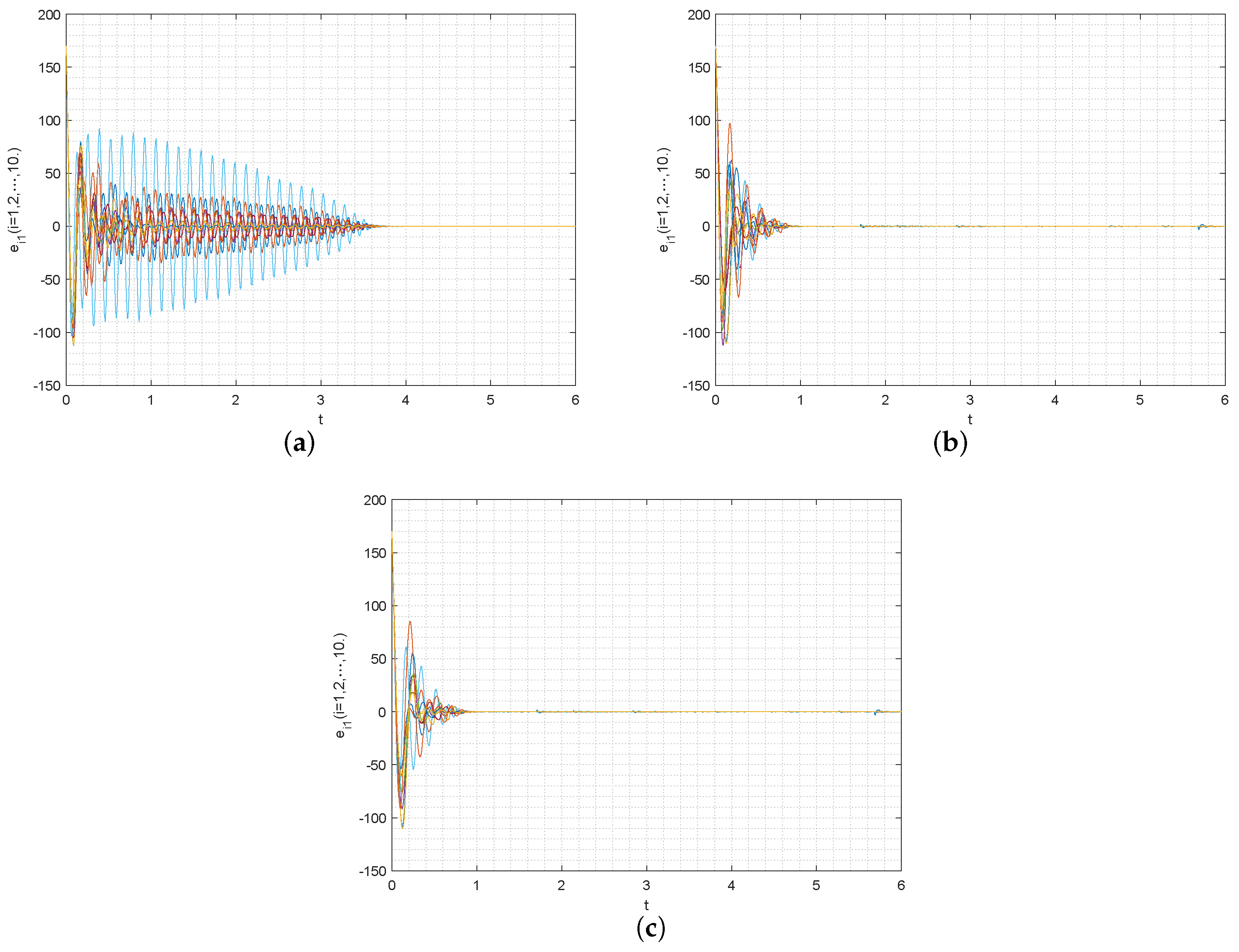
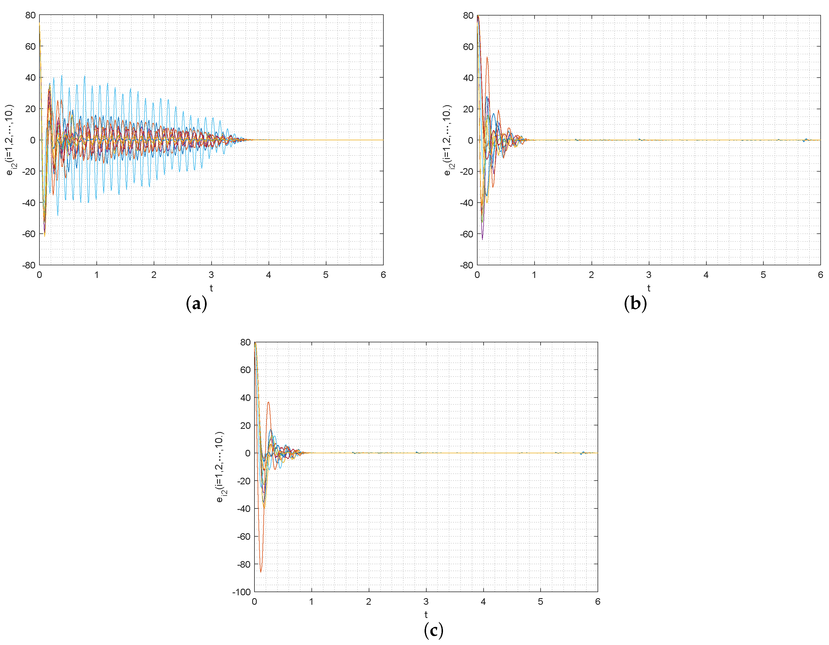
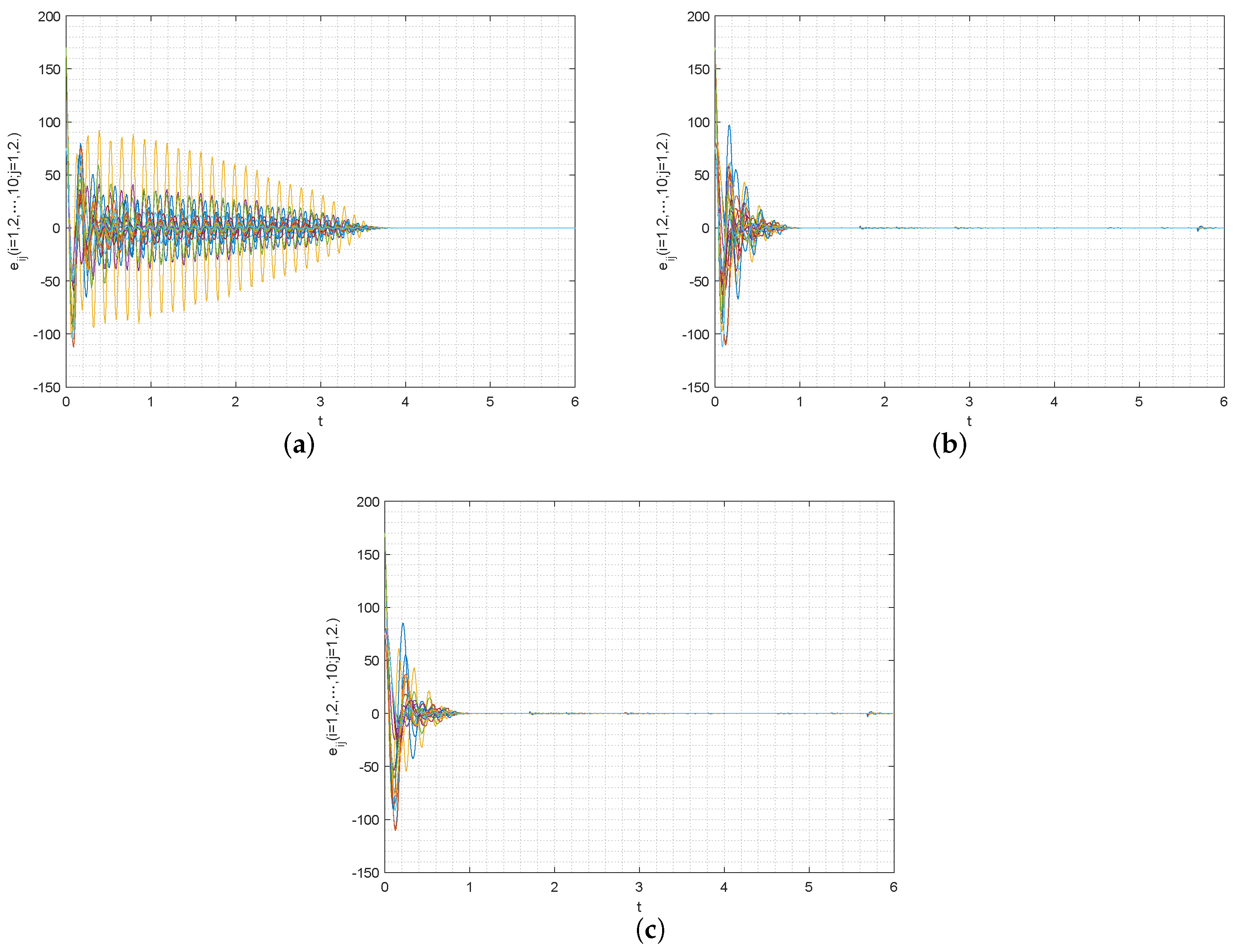
4. Numerical Simulation

In this section, by employing MATLAB R2020a and the Admas–Bashforth–Moulton predictor corrector method, the effectiveness and validity of the methods are confirmed through a numerical example.

Example 1.

Suppose that the FONCDNUP mentioned below consists of a total of n nodes, and it is designed as follows

$${ }_{t0}^c{D}_t^{\alpha }{\varphi }_i(t)=G_0{\varphi }_i(t)+B_0\hslash ({\varphi }_i(t))+c\sum _{j=1}^N{d}_{ij}\Lambda {\varpi }_j(t),$$

and

$${ }_{t0}^c{D}_t^{\alpha }{\phi }_i(t)=(A_0+\Delta A(t)){\phi }_i(t)+(D_0+\Delta D(t))\hslash ({\phi }_i(t))+c\sum _{j=1}^N{d}_{ij}\Lambda s_j(t)+u_i(t).$$

Then, the controller is

$$\left\{\begin{array}{cc}\hfill u_{i1}(t)& =-(A_0+\Delta A(t)-G_0){\varphi }_i(t)-(D_0+\Delta D(t))\hslash ({\varphi }_i(t))+B_0\hslash ({\varphi }_i(t))-\varpi \frac{e_i(t)}{\parallel e_i{(t)\parallel }^{\varrho }},\hfill \\ \hfill u_{i2}(t)& =u_{i1}(t)-\widehat{\lambda }{u}_{i3},\hfill \\ \hfill u_{i3}(t)& ={\delta }_i{e}_i(t),\hfill \\ \hfill u_{i4}(t)& =u_{i1}(t)-\lambda u_{i3},\hfill \end{array}\right.$$

where $\alpha =0.99$, $\delta =9$, $\lambda =1$, $\varpi =0.02$, $\varrho =2.1$, ${\varphi }_i(t)={[{\varphi }_{i1},{\varphi }_{i2}]}^{\top }$, ${\phi }_i(t)={[{\phi }_{i1},{\phi }_{i2}]}^{\top }$, $i=1,2,\cdots ,10$, $c=7.25$, $h=3.55,f=18.1$, and the nonlinear functions can be expressed as $\hslash ({\varphi }_i(t))={[h*tanh({\varphi }_{i1}(t)),h*tanh({\varphi }_{i2}(t))]}^{\top }$; $\hslash ({\phi }_i(t))={[f*tanh({\phi }_{i1}(t)),f*tanh({\phi }_{i2}(t))]}^{\top }.$

And the parameters matrices are as follows:

$$G_0=\left(\begin{array}{cc}-45.5& -47\\ -5.01& -105.01\end{array}\right),B_0=\left(\begin{array}{cc}-0.5& -1\\ -0.2& -4.05\end{array}\right).$$

$$A_0=\left(\begin{array}{cc}3.05& 20\\ 8& 3.55\end{array}\right),D_0=\left(\begin{array}{cc}-0.551& 8.032\\ 5.08& -5.25\end{array}\right).$$

The internal coupling and outer coupling matrices are defined as follows, respectively,

$$\Lambda =\left(\begin{array}{cc}0.25& 0\\ 0& 0.25\end{array}\right),$$

$${(d_{ij})}_{n\times n}=\left(\begin{array}{cccccccccc}-2& 1& 0& 1& 0& 0& 0& 0& 0& 0\\ 0& -2& 1& 0& 1& 0& 0& 0& 0& 0\\ 1& 0& -3& 0& 0& 1& 1& 0& 0& 0\\ 0& 0& 1& -1& 0& 0& 0& 0& 0& 0\\ 0& 1& 0& 1& -3& 0& 0& 0& 1& 0\\ 1& 0& 0& 0& 0& -1& 0& 0& 0& 0\\ 0& 1& 0& 0& 0& 0& -1& 0& 0& 0\\ 1& 1& 0& 0& 0& 0& 0& -2& 0& 0\\ 1& 0& 1& 0& 0& 0& 0& 0& -2& 0\\ 0& 0& 1& 0& 0& 0& 0& 0& 0& -1\end{array}\right).$$

Then, the uncertain parameters matrices are

$M_a=\left(\begin{array}{cc}0.1& 0\\ 0& 0.5\end{array}\right),H_a=\left(\begin{array}{cc}0.2& 0\\ 0& 0.1\end{array}\right),$$F_e(t)=\left(\begin{array}{cc}cos({\varpi }_1(t))& 0\\ 0& cos({\varpi }_2(t))\end{array}\right),$ and $M_d=\left(\begin{array}{cc}1& 0\\ 0& 0.9\end{array}\right),H_d=\left(\begin{array}{cc}1& 0\\ 0& 0.9\end{array}\right),$$F_g(t)=\left(\begin{array}{cc}0.41cos(s_1(t))& 0\\ 0& cos(s_2(t))\end{array}\right).$

As per the above the numerical simulations, Figure 1 represents the synchronization error trajectory of error system $e_{i1}$ with controllers $u_{i1}$, $u_{i2}$, and $u_{i4}$, respectively. Figure 2 represents the synchronization error trajectory of error system $e_{i2}$ with controllers $u_{i1}$, $u_{i2}$, and $u_{i4}$, respectively. Figure 3 represents the total synchronization error trajectory of error system $e_{ij},(i=1,2,\cdots ,10;j=1,2.)$ with controllers $u_{i1}$, $u_{i2}$, and $u_{i4}$, respectively. Figure 4 represents the total synchronization error trajectory of $\parallel e(t)\parallel =({\sum }_{i=1}^{10}|e_i(t){{|}_2^2)}^{\frac{1}{2}}$ with controllers $u_{i1}$, $u_{i2}$, and $u_{i4}$, respectively. It can be obtained from Figure 1, Figure 2, Figure 3 and Figure 4, where b represents the error trajectory of the error system $e_{ij},(i=1,2,\cdots ,10;j=1,2.)$ under the new controller $u_{i2}$ and a represents the error trajectory of the error system $e_{ij},(i=1,2,\cdots ,10;j=1,2.)$ under the general controller $u_{i1}$. Comparing b and a, it can be obtained that the control effect of b is better than that of a, but there is little difference compared with the comparison group c, thus proving that the control effect of $u_{i2}$ is better.

5. Conclusions

In this paper, we have researched the FTS problem of FONCNUPs. Firstly, the model takes into account non-isomorphism and parameter uncertainties and then proposes a new synchronization criterion to address the FTS problem of FONCNUPs. Additionally, a new controller is designed to minimize control costs and enhance control efficiency. Finally, we demonstrate the effectiveness of our results through two numerical examples. Our conclusions will have equally good effects on fractional-order complex networks with similar problems, and our conclusions have lower conservatism. It can be applied to many situations. However, the current study does not consider the case of time delays, which is also significant in the study of complex networks. And the results of this paper cannot be directly applied to fractional complex networks with delay. Therefore, in future research, we can focus on extending the proposed methods to encompass fractional-order complex networks with time delays.

References

1. Shahal, S.; Wurzberg, A.; Sibony, I.; Duadi, H.; Shniderman, E.; Weymouth, D.; Davidson, N.; Fridman, M. Synchronization of complex human networks. Nat. Commun. 2020, 11, 3854. [Google Scholar] [CrossRef]
2. Luarn, P.; Yang, J.C.; Chiu, Y.P. The network effect on information dissemination on social network sites. Comput. Hum. Behav. 2014, 37, 1–8. [Google Scholar] [CrossRef]
3. Zhou, Q.; Wei, D.Q. Collective dynamics of neuronal network under synapse and field coupling. Nonlinear Dyn. 2021, 105, 753–765. [Google Scholar] [CrossRef]
4. Liu, F.Y.; Yang, Y.Q.; Chang, Q. Synchronization of fractional-order delayed neural networks with reaction-diffusion terms: Distributed delayed impulsive control. Commun. Nonlinear Sci. Numer. Simul. 2023, 124, 107303. [Google Scholar] [CrossRef]
5. Yu, J.; Hu, C.; Jiang, H.J.; Fan, X.L. Projective synchronization for fractional neural networks. Neural Netw. 2014, 49, 87–95. [Google Scholar] [CrossRef] [PubMed]
6. Majidabad, S.S.; Shandiz, H.T.; Hajizadeh, A. Nonlinear fractional-order power system stabilizer for multi-machine power systems based on sliding mode technique. Int. J. Robust Nonlinear Control 2015, 25, 1548–1568. [Google Scholar] [CrossRef]
7. Chen, W.; Zhou, B. Controllability of flow-conservation transportation networks with fractional-order dynamics. Complexity 2021, 2021, 8524984. [Google Scholar] [CrossRef]
8. Podlubny, I. Fractional Differential Equations; Academic Press: San Diego, CA, USA, 1999. [Google Scholar]
9. Tao, B.B.; Xiao, M.; Sun, Q.S.; Cao, J.D. Hopf bifurcation analysis of a delayed fractional-order genetic regulatory network model. Neurocomputing 2018, 275, 677–686. [Google Scholar] [CrossRef]
10. Sun, H.; Duan, J.; Xu, T. Analytical solutions of fractional order chemical engineering equations by a new fractional sub-equation method. Chem. Eng. Sci. 2020, 214, 115399. [Google Scholar]
11. Das, M.; Samanta, G.P. A delayed fractional order food chain model with fear effect and prey refuge. Math. Comput. Simul. 2020, 178, 218–245. [Google Scholar] [CrossRef]
12. Gibson, J.; Beierlein, M.; Connors, B. Two networks of electrically coupled inhibitory neurons in neocortex. Nature 1999, 402, 75–79. [Google Scholar] [CrossRef]
13. Creo, S.; Lancia, M.R.; Vernole, P. Convergence of fractional diffusion processes in extension domains. J. Evol. Eq. 2020, 20, 109–139. [Google Scholar] [CrossRef]
14. Jiang, Y.W.; Zhang, B.; Shu, X.J.; Wei, Z.H. Fractional-order autonomous circuits with order larger than one. J. Adv. Res. 2020, 25, 217–225. [Google Scholar] [CrossRef]
15. Fan, Y.; Huang, X.; Wang, Z.; Li, Y. Nonlinear dynamics and chaos in a simplified memristor-based fractional-order neural network with discontinuous memductance function. Nonlinear Dyn. 2018, 93, 611–627. [Google Scholar] [CrossRef]
16. Shukla, M.K.; Sharma, B.B. Secure communication and image encryption scheme based on synchronisation of fractional order chaotic systems using backstepping. Int. J. Simul. Process. Model. 2018, 13, 473–485. [Google Scholar] [CrossRef]
17. Li, H.; Zhang, L.; Hu, C.; Jiang, Y.; Teng, Z. Dynamical analysis of a fractional-order predator-prey model incorporating a prey refuge. J. Appl. Math. Comput. 2017, 54, 435–449. [Google Scholar] [CrossRef]
18. Povstenko, Y.Z. Fractional radial heat conduction in an infinite medium with a cylindrical cavity and associated thermal stresses. Mech. Res. Commun. 2010, 37, 436–440. [Google Scholar] [CrossRef]
19. Huang, J.; Shen, T. Well-posedness and dynamics of the stochastic fractional magneto-hydrodynamic equations. Nonlinear Anal. Theory Methods Appl. 2016, 133, 102–133. [Google Scholar] [CrossRef]
20. Ding, Z.; Chen, C.; Wen, S.; Li, S.; Wang, L. Lag projective synchronization of nonidentical fractional delayed memristive neural networks. Neurocomputing 2022, 469, 138–150. [Google Scholar] [CrossRef]
21. Yang, L.X.; Jiang, J. Adaptive synchronization of drive-response fractional-order complex dynamical networks with uncertain parameters. Commun. Nonlinear Sci. Numer. Simul. 2014, 19, 1496–1506. [Google Scholar] [CrossRef]
22. Roohi, M.; Zhang, C.; Chen, Y. Adaptive model-free synchronization of different fractional-order neural networks with an application in cryptography. Nonlinear Dyn. 2020, 100, 3979–4001. [Google Scholar] [CrossRef]
23. Prakash, M.; Balasubramaniam, P.; Lakshmanan, S. Synchronization of Markovian jumping inertial neural networks and its applications in image encryption. Neural Netw. 2016, 83, 86–93. [Google Scholar] [CrossRef]
24. Syed, A.M.; Hymavathi, M.; Senan, S.; Shekher, V.; Arik, S. Global asymptotic synchronization of impulsive fractional-order complex-valued memristor-based neural networks with time varying delays. Commun. Nonlinear Sci. Numer. Simul. 2019, 78, 104869. [Google Scholar] [CrossRef]
25. Wang, F.; Yang, Y.Q. Quasi-synchronization for fractional-order delayed dynamical networks with heterogeneous nodes. Appl. Math. Comput. 2018, 339, 1–14. [Google Scholar] [CrossRef]
26. Kao, Y.G.; Li, Y.; Park, J.H.; Chen, X.Y. Mittag-Leffler synchronization of delayed fractional memristor neural networks via adaptive control. IEEE Trans. Neural Netw. Learn. Syst. 2021, 32, 2279–2284. [Google Scholar] [CrossRef]
27. Li, L.; Chen, W.S.; Wu, X.J. Global exponential stability and synchronization for novel complex-valued neural networks with proportional delays and inhibitory factors. IEEE Trans. Cybern. 2021, 51, 2142–2152. [Google Scholar] [CrossRef]
28. Jia, Y.; Wu, H. Global synchronization in finite time for fractional-order coupling complex dynamical networks with discontinuous dynamic nodes. Neurocomputing 2019, 358, 20–32. [Google Scholar] [CrossRef]
29. Yang, S.; Hu, C.; Yu, J.; Jiang, H. Finite-time cluster synchronization in complex-variable networks with fractional-order and nonlinear coupling. Neural Netw. 2021, 135, 212–224. [Google Scholar] [CrossRef]
30. Li, Y.; Kao, Y.G.; Wang, C.H.; Xia, H.W. Finite-time synchronization of delayed fractional-order heterogeneous complex networks. Neurocomputing 2020, 384, 368–375. [Google Scholar] [CrossRef]
31. Xiao, J.; Wu, L.; Wu, A.L.; Zeng, Z.G.; Zhang, Z. Novel controller design for finite-time synchronization of fractional-order memristive neural networks. Neurocomputing 2022, 512, 494–502. [Google Scholar] [CrossRef]
32. Li, H.L.; Hu, C.; Zhang, L.; Jiang, H.J.; Cao, J.D. Complete and finite-time synchronization of fractional-order fuzzy neural networks via nonlinear feedback control. Fuzzy Sets Syst. 2022, 443, 50–69. [Google Scholar] [CrossRef]
33. Li, H.L.; Hu, C.; Zhang, L.; Jiang, H.J.; Cao, J.D. Non-separation method-based robust finite-time synchronization of uncertain fractional-order quaternion-valued neural networks. Appl. Math. Comput. 2021, 409, 126377. [Google Scholar] [CrossRef]
34. Xu, Y.; Li, Y.; Li, W. Adaptive finite-time synchronization control for fractional-order complex-valued dynamical networks with multiple weights. Commun. Nonlinear Sci. Numer. Simul. 2020, 85, 105239. [Google Scholar] [CrossRef]
35. Arslan, E.; Narayanan, G.; Syed, A.M.; Arik, S.; Saroha, S. Controller design for finite-time and fixed-time stabilization of fractional-order memristive complex-valued BAM neural networks with uncertain parameters and time-varying delays. Neural Netw. 2020, 130, 60–74. [Google Scholar] [CrossRef]
36. Du, F.F.; Lu, J.G.; Zhang, Q.H. Delay-dependent finite-time synchronization criterion of fractional-order delayed complex networks. Commun. Nonlinear Sci. Numer. Simul. 2023, 119, 107072. [Google Scholar] [CrossRef]
37. Zhang, S.; Yu, Y.; Wang, H. Mittag-Leffler stability of fractional-order hopfield neural networks. Nonlinear Anal. Hybrid Syst. 2015, 16, 104–121. [Google Scholar] [CrossRef]
38. Xu, S.; Lam, J.; Ho, D.W.; Zou, Y. Global robust exponential stability analysis for interval recurrent neural networks. Phys. Lett. A 2004, 325, 124–133. [Google Scholar] [CrossRef]
Figure 1. (ac) represent the synchronized error trajectories of system e i 1 ( i = 1 , , 10 ) with the controller u i 1 , controller u i 2 , and controller u i 4 , respectively.
Fractalfract 08 00155 g001
Figure 2. (ac) represent the synchronized error trajectories of system e i 2 ( i = 1 , , 10 ) with the controller u i 1 , controller u i 2 , and controller u i 4 , respectively.
Fractalfract 08 00155 g002
Figure 3. (ac) represent the synchronized error trajectories of system e i j ( i = 1 , , 10 ; j = 1 , 2 . ) with the controller u i 1 , controller u i 2 , and controller u i 4 , respectively.
Fractalfract 08 00155 g003
Figure 4. (ac) represent the total synchronized error trajectories of e ( t ) = ( i = 1 10 | e i ( t ) | 2 2 ) 1 2 with the controller u i 1 , controller u i 2 , and controller u i 4 , respectively.
Fractalfract 08 00155 g004
Disclaimer/Publisher’s Note: The statements, opinions and data contained in all publications are solely those of the individual author(s) and contributor(s) and not of MDPI and/or the editor(s). MDPI and/or the editor(s) disclaim responsibility for any injury to people or property resulting from any ideas, methods, instructions or products referred to in the content.