A Fractional Heston-Type Model as a Singular Stochastic Equation Driven by Fractional Brownian Motion

Abstract

This paper introduces the fractional Heston-type (fHt) model as a stochastic system comprising the stock price process modeled by a geometric Brownian motion. In this model, the infinitesimal return volatility is characterized by the square of a singular stochastic equation driven by a fractional Brownian motion with a Hurst parameter $H\in (0,1)$. We establish the Malliavin differentiability of the fHt model and derive an expression for the expected payoff function, revealing potential discontinuities. Simulation experiments are conducted to illustrate the dynamics of the stock price process and option prices.

1. Introduction

Allowing volatility to be stochastic in a financial market model was one of the great achievements in the history of quantitative finance. This innovation led to stochastic volatility modeling, as previously discussed by Heston [1] and several other researchers, addressing shortcomings in the standard Black–Scholes model (see, for example, Alos et al. [2] for a summary). In the context of Heston [1], the stock price process is described by a geometric Brownian motion of the form:

$$d{S}_t=\eta S_{t}dt+\sqrt{Y_t}{S}_{t}d{B}_t,$$

where $\eta$ and ${\left(Y_t\right)}_{t\ge 0}$ represent a constant drift and the stochastic variance of the instantaneous rate of return $d{X}_t:=d{S}_t/S_t$, respectively. The stochastic process ${\left(Y_t\right)}_{t\ge 0}$ takes the form of the standard Cox–Ingersoll–Ross process, satisfying the following stochastic differential equation:

$$d{Y}_t=\theta (\mu -Y_t)dt+\nu \sqrt{Y_t}d\tilde{B}\left(t\right).$$

The parameter $\theta$ represents the speed of reversion of the stochastic process ${\left(Y_t\right)}_{t\ge 0}$ towards its long-run mean $\mu$, and the parameter $\nu$ represents the volatility of the stochastic variance ${\left(Y_t\right)}_{t\ge 0}$. The Brownian motions ${\left(B_t\right)}_{t\ge 0}$ and ${\left({\tilde{B}}_t\right)}_{t\ge 0}$ are assumed to be correlated. This model is well known in the literature as the Heston model.

It has recently been demonstrated that volatility and the volatility of volatility exhibit rough behaviors. This implies that the paths tend to be rougher, showing short-range dependency and can be effectively modelled using fractional Brownian motion with a Hurst parameter $H<1/2$. For further insights, refer to studies such as Alos et al. [3], Fukasawa [4], Gatheral et al. [5], Livieri et al. [6], Takaishi [7], Fukasawa [8], Brandi and Di Matteo [9], and related findings.

On the other hand, volatility persistence is also associated with long-memory properties, indicated by the slow decay of the autocorrelation function. In this regard, Comte and Renault [10] demonstrated that long-memory stochastic volatility models are better suited to reproduce the gradual flattening of implied volatility skews and smiles observed in financial market data. This finding has been corroborated and tested by several other researchers, including Chronopoulou and Viens [11], Chronopoulou and Viens [12], Tripathy [13], and subsequent studies. In contrast to rough volatility, this modeling approach involves using fractional Brownian motion with a Hurst parameter $H>1/2$.

From the above, we may notice a contradiction regarding whether volatility is rough or exhibits long-range dependency, a subject of debate in the literature. However, Alos and Lorite [14] observed that both properties are not mutually exclusive. A process can exhibit both long and short dependency properties, with each dominating at different scales, and consequently, at different maturities in the implied volatility surface. This idea is supported by Funahashi and Kijima [15], who demonstrated that if the volatility ${\sigma }_t=f(Y_t^H+Y_t^{H^{\prime }})$ where $Y_t^H$ and $Y_t^{H^{\prime }}$ are the fractional Ornstein–Uhlenbeck process driven by fractional Brownian motions with Hurst parameters $H>1/2$ and $H^{\prime }<1/2$, respectively, then $Y_t^H$ does not have an impact on the ATM short-time limit skew.

To incorporate both roughness and long-range dependency properties into the Heston model, the standard Brownian motion is replaced by a fractional Brownian motion ${\left(W_t^H\right)}_{t\ge 0}$ with a Hurst parameter $H>1/2$ or $H<1/2$, resulting in the fractional Heston model. For further details, refer to studies such as Alos and Yang [16], Mishura and Yurchenko-Tytarenko [17], Mehrdoust and Fallah [18], Tong and Liu [19], Richard et al. [20], along with the references therein. In this context, the volatility process can be represented by:

$$d{Y}_t=\theta (\mu -Y_t)dt+\nu \sqrt{Y_t}d{W}_t^H.$$

(1)

The stochastic process ${\left(Y_t\right)}_{t\ge 0}$ is well-known as the fractional Cox–Ingersoll–Ross (fCIR) process. The Equation (1) is well defined only when $H\in (2/3,1)$ as shown by Mishura et al. [21]. This limitation was overcome by defining fCIR process as a square of a stochastic process with additive fBm. In other words, the stochastic process ${\left(Y_t\right)}_{t\ge 0}$ can be written as the square of a stochastic process ${\left(Z_t\right)}_{t\ge 0}$ that verifies

$$d{Z}_t=\frac{1}{2}\left(\frac{\mu }{Z_t}-\theta Z_t\right)dt+\frac{\nu }{2}d{W}_t^H.$$

(2)

The stochastic volatility process ${\left(Y_t\right)}_{t\ge 0}$ described above gives rise to complex models in option pricing or risk analysis, which are not easily manageable, particulary when the volatility drift is not constant. In this paper, we propose a general form of the fractional Heston-type model in a simple and natural manner. As before, we assume that the stock price process is driven by a geometric Brownian motion ${\left(S_t\right)}_{t\ge 0}$, satisfying the following stochastic differential equation:

$$d{S}_t=\eta S_{t}dt+\sigma \left(Y_t\right)S_{t}d{B}_t,$$

(3)

where $\sigma \left(Y_t\right)$ represents the volatility of the infinitesimal log-return $d{X}_t:=d{S}_t/S_t$ with ${\left(Y_t\right)}_{t\ge 0}$ a fractional Cox–Ingersoll–Ross (fCIR) process that captures both long and short-range dependency. We adopt the definition provided by Mishura and Yurchenko-Tytarenko [22] or Mpanda et al. [23] and describe the stochastic process ${\left(Y_t\right)}_{t\ge 0}$ as

$$Y_t\left(\omega \right)=Z_t^2\left(\omega \right){\mathbf{1}}_{[0,\tau (\omega \left)\right)},\forall t\ge 0,\omega \in \Omega ,$$

(4)

where the stochastic process ${\left(Z_t\right)}_{t\ge 0}$ is referred to as a general form of the fCIR process that satisfies the following differential equation:

$$d{Z}_t=\frac{1}{2}\left(f(t,Z_t)Z_t^{-1}dt+\nu d{W}_t^H\right),\nu >0,$$

(5)

and $\tau$ is the first time the process ${\left(Z_t\right)}_{t\ge 0}$ hits zero, defined by

$$\tau \left(\omega \right)=inf\left\{t>0:Z_t\left(\omega \right)=0\right\}.$$

(6)

It was shown in Mpanda et al. [23] that the stochastic process ${\left(Y_t\right)}_{t\ge 0}$ satisfies $d{Y}_t=f(t,Y_t)dt+\nu \sqrt{Y_t}\circ d{W}_t^H$. This implies that the function $f(t,z)$ can be defined as the drift of the volatility process ${\left(Y_t\right)}_{t\ge 0}$. Additionally, the stochastic process ${\left(W_t^H\right)}_{t\ge 0,H\in (0,1)}$ is well-known as fractional Brownian motion (fBm) with Hurst parameter H, defined as a centered Gaussian process with a covariance function:

$$E\left[W_t^H{W}_s^H\right]=\frac{1}{2}\left(t^{2H}+s^{2H}-\mid t-s{\mid }^{2H}\right),\forall s,t\ge 0.$$

(7)

There exist several representations of fBm. Nourdin [24] summarized them. In financial volatility modelling, the Volterra representation is widely used, particulary due to its simplicity. In this representation, the fBm is written in terms of a standard Brownian motion in the time interval $[0,t]$ as follows:

$$W_t^H={\int }_0^t{\kappa }_H(s,t)d{V}_t,$$

(8)

where ${\left(V_t\right)}_{t\in [0,T]}$ is a standard Brownian motion and where ${\kappa }_H(s,t)$ is a square integrable kernel that may take different forms. One effective expression is through the Euler hypergeometric integral with ${\kappa }_H(s,t)$ given by

$${\kappa }_H(t,s)=\frac{{(t-s)}^{H-\frac{1}{2}}}{\Gamma (H+\frac{1}{2})}{ }_2{\mathbf{F}}_1\left(H-\frac{1}{2};\frac{1}{2}-H;H+\frac{1}{2};1-\frac{t}{s}\right){\mathbf{1}}_{[0,t]}\left(s\right),\forall s\in [0,t],$$

(9)

with $\Gamma (·)$ and ${ }_2{\mathbf{F}}_1(a,b,c;d)$ being the gamma and Gaussian hypergeometric functions, respectively. A truncated expression of the kernel (9) was suggested by Decreusefond and Üstünel [25] where ${ }_2{\mathbf{F}}_1\left(H-\frac{1}{2};\frac{1}{2}-H;H+\frac{1}{2};1-\frac{t}{s}\right){\mathbf{1}}_{[0,t]}\left(s\right)\approxeq 1$. This representation is referred to as a Type II fBm or Riemann–Liouville fBm. Here, ${\kappa }_H(s,t)$ is defined by

$${\kappa }_H(t,s)=\frac{1}{\Gamma (H+\frac{1}{2})}{(t-s)}^{H-\frac{1}{2}}.$$

(10)

This representation was used by Gatheral et al. [5] to model rough volatility. The standard Brownian motions ${\left(B_t\right)}_{t\in [0,T]}$ and ${\left(V_t\right)}_{t\in [0,T]}$ are assumed to be correlated, meaning there exists $\rho \in [-1,1]$ such that $E\left[B_t{V}_t\right]=\rho t.$ This implies that there exists a Brownian motion ${\left({\tilde{V}}_t\right)}_{t\in [0,T]}$ independent to ${\left(V_t\right)}_{t\in [0,T]}$, that is $E\left[V_t,{\tilde{V}}_t\right]=0$, such that

$$B_t=\rho V_t+\sqrt{1-{\rho }^2}{\tilde{V}}_t.$$

(11)

A new and natural way of defining a fractional Heston-type (fHt) model as singular stochastic differential equation driven by a fractional Brownian motion is through the following stochastic system:

$$\left\{\begin{array}{c}d{X}_t=\eta dt+\sigma \left(Y_t\right)d{B}_t,\hfill \\ Y_t=Z_t^2{\mathbf{1}}_{[0,\tau (\omega \left)\right]}\hfill \\ d{Z}_t=\frac{1}{2}f(t,Z_t)Z_t^{-1}dt+\frac{1}{2}\nu d{W}_t^H\hfill \\ W_t^H={\int }_0^t{\kappa }_H(s,t)d{V}_t\hfill \\ B_t=\rho V_t+\sqrt{1-{\rho }^2}{\tilde{V}}_t\hfill \end{array}\right.$$

(12)

The existence of the stochastic process ${\left(Z_t\right)}_{t\ge 0}$ in (5) was previously discussed by Nualart and Ouknine [26]. They proposed that for $H<1/2$, the drift function $g(t,z):=f(t,z)z^{-1}$ must satisfy the linear growth condition, and for $H>1/2$, $g(t,z)$ must verify the Hölder continuity condition. Additionally, particular cases of fHt model (12) has been previously investigate by Alos and Yang [16], Mishura and Yurchenko-Tytarenko [17], Bezborodov et al. [27] for $H>1/2$. One can use the same idea of Bezborodov et al. [27] (Theorem 3.6) to show that the fHt model is free of arbitrage. The above stochastic model is also a generalisation of the rough volatility model previously discussed by Gatheral et al. [5] with $\sigma \left(y\right)=e^y$, $f(t,y)=-\theta y$ and the Type II fBm of the form (10) with small Hurst parameters.

The remainder of this paper is structured as follows: Section 2 constructs approximating sequences of stock prices and fCIR processes. Malliavin differentiability within the fHt model is discussed in Section 3. Finally, Section 4 derives the expected payoff function and performs simulations of option prices.

2. Approximating Sequences in fHt Model

The main purpose of introducing approximating sequences of both fractional volatility and stock price processes relies on their positiveness. The following theorems discuss the positiveness of ${\left(Z_t\right)}_{t\ge 0}$ and before this, we consider the following assumption below.

Assumption 1.

(i) 

The function $g:[0,\infty )\times (0,\infty )\to (-\infty ,\infty )$ defined by $g(t,z):=f(t,z)/z$ is continuous and admits a continuous partial derivative with respect to x on $(0,\infty )$.

(ii) 

for any $T>0$, there exists $z_T>0$ such that

$$f(t,z)>0forall0<t\le Tand0\le z\le z_T.$$

Under this assumption, the following theorems follow.

Theorem 1.

Let ${\left(Z_t\right)}_{t\ge 0}$ be a stochastic process that verifies (5) with $H>\frac{1}{2}$ and $f:[0,\infty )\times [0,\infty )$ is a continuous function that satisfies Assumption 1. Then,

$$P\{\omega \in \Omega :\tau (\omega )=\infty \}=1,$$

where $\tau \left(\omega \right)=inf\{t>0:Z_t\left(\omega \right)=0\}.$

Proof. 

Here, we highlight the proof of this theorem by contradiction, and we refer the reader to Mpanda et al. [23] for a complete and comprehensive proof. Let $\tau \left(\omega \right)=inf\{t\ge 0:Z_t\left(\omega \right)=0\}$ be the first time that the process ${\left(Z_t\right)}_{t\in [0,T]}$ hits zero and ${\tau }_{\epsilon }\left(\omega \right)=sup\{t\in (0,\tau \left(\omega \right)):Z_t\left(\omega \right)=\epsilon \}$ be the last time $\left(Z_t\right)$ hits $\epsilon$ before reaching zero. In addition, define

$$A=inf\{g(t,z):\zeta \le t\le T\mathrm{and}0\le z\le z_0\},$$

where $g(t,z)=f(t,z)z^{-1}$ and $z_0$ is any point chosen between zero and the initial value of ${\left(Z_t\right)}_{t\in [0,T]}$, that is, $0<z_0<Z_0$ and $\zeta =inf\{t\ge 0:Z_t\left(\omega \right)=z_0\}$. Then, from (5), we have:

$$Z_{\tau }-Z_{{\tau }_{\epsilon }}=\frac{1}{2}{\int }_{\tau }^{{\tau }_{\epsilon }}g(s,Z_s)ds+\frac{\nu }{2}(W_{\tau }^H-W_{{\tau }_{\epsilon }}^H)=-\epsilon$$

and by Hölder continuity of fBm, we have

$$\nu |W_{\tau }^H-W_{{\tau }_{\epsilon }}^H|=2\epsilon +{\int }_{\tau }^{{\tau }_{\epsilon }}g(s,Z_s)ds\le c\nu {|\tau -{\tau }_{\epsilon }|}^{H-\alpha },$$

which yields the following inequality

$$A{\epsilon }^{-1}(\tau -{\tau }_{\epsilon })-c\nu {|\tau -{\tau }_{\epsilon }|}^{H-\alpha }+2\epsilon \le 0$$

for some constant $c>0$. Define

$$F_{\epsilon }\left(z\right)=A{\epsilon }^{-1}z-c\nu z^{H-\alpha }+2\epsilon ,$$

then we have

$$F_{\epsilon }(\tau -{\tau }_{\epsilon })\le 0.$$

(13)

On the other hand, the critical point $\widehat{z}$ of the function $F_{\epsilon }\left(z\right)$ is given by

$$\widehat{z}={\left(\frac{A{\epsilon }^{-1}}{c\nu (H-\alpha )}\right)}^{\frac{1}{H-\alpha -1}}$$

and

$$F_{\epsilon }\left(\widehat{z}\right)\ge -\kappa {\epsilon }^q+2\epsilon ,$$

where

$$\kappa =(H-\alpha -1){\left(\frac{A{\epsilon }^{H-\alpha }}{c\nu {(H-\alpha )}^{-H+\alpha +2}}\right)}^{\frac{1}{H-\alpha -1}}$$

and

$$q=-\frac{H-\alpha }{H-\alpha -1}.$$

One may notice that there exists $0<\epsilon <{\epsilon }^{*}$ such that $F_{\epsilon }\left(\widehat{z}\right)\ge -\kappa {\epsilon }^q+2\epsilon >0$ for all $H>1/2$. This goes in contradiction with (13). □

Theorem 2.

Consider for each $k>0$, the stochastic process ${\left(Z_t^{\left(k\right)}\right)}_{t\ge 0}$ defined by

$$\begin{array}{c}\hfill Z_t^{\left(k\right)}=\left\{\begin{array}{cc}{Z}_0+{\int }_0^t{\displaystyle \frac{f_k(t,Z_s^{\left(k\right)})}{Z_s^{\left(k\right)}}}ds+{\displaystyle \frac{\nu }{2}}{W}_t^H\hfill & if t<{\tau }^{\left(k\right)}\left(\omega \right)\hfill \\ 0\hfill & otherwise,\hfill \end{array}\right.\end{array}$$

where ${\tau }^{\left(k\right)}\left(\omega \right)=inf\{t\ge 0:Z_t^{\left(k\right)}\left(\omega \right)=0\}.$ Then, for any $T>0$ and $H<1/2$,

$$P(\omega \in \Omega :{\tau }^{\left(k\right)}\left(\omega \right)>T)\to 1ask\to \infty .$$

Proof. 

The proof can be carried out as previously shown by defining ${\tau }_{\epsilon }^{\left(k_n\right)}\left(\omega \right)=sup\{t\in (0,\tau \left(\omega \right)):Z_t^{\left(k_n\right)}\left(\omega \right)=\epsilon \}$ and $A_k=inf\{g_k(t,z):\zeta \le t\le T\mathrm{and}0\le z\le z_0\},$ where $g_k(t,z)=f_k(t,z)z^{-1}k>0.$ For more details, refer to Mpanda et al. [23]. □

2.1. Approximating Sequences of ${\left(Z_t\right)}_{t\ge 0}$

Inspired by Alos and Ewald [28], we construct an approximating sequence ${\left(Z_t^{\epsilon }\right)}_{t\ge 0,\epsilon >0}$ of the fCIR process that satisfies the following differential equation:

$$d{Z}_t^{\epsilon }=\frac{1}{2}f(t,Z_t^{\epsilon }){\Lambda }_{\epsilon }\left(Z_t^{\epsilon }\right)dt+\frac{\sigma }{2}d{W}_t^H,Z_0^{\epsilon }=Z_0>0,$$

(14)

where the function ${\Lambda }_{\epsilon }\left(z\right)$ in (14) is defined by

$${\Lambda }_{\epsilon }\left(z\right)={(z{\mathbf{1}}_{\{z>0\}}+\epsilon )}^{-1}.$$

(15)

It is easy to verify that ${\Lambda }_{\epsilon }\left(z\right)>0$ for all $\epsilon >0$. As a straight consequence, the drift of ${\left(Z_t^{\epsilon }\right)}_{t\ge 0,\epsilon >0}$ is also positive. In addition, ${lim}_{z\to 0}{\Lambda }_{\epsilon }\left(z\right)={\epsilon }^{-1}$, ${lim}_{z\to \infty }{\Lambda }_{\epsilon }\left(z\right)=0$, ${lim}_{\epsilon \to 0}{\Lambda }_{\epsilon }\left(z\right)=z^{-1}:=\Lambda \left(z\right)$ and

$${\Lambda }_{\epsilon }^{\prime }\left(z\right)=\left\{\begin{array}{cc}\hfill 0,& \mathrm{if}z<0\hfill \\ \hfill -\frac{1}{{(z+\epsilon )}^2},& \mathrm{if}z>0\hfill \end{array}\right.$$

(16)

The next step is to show that for every $t\ge 0$, the sequence $Z_t^{\epsilon }$ converges to $Z_t$ in $L^p$ as $\epsilon \to 0$.

Proposition 3.

The sequence of estimated random variables $Z_t^{\epsilon }$ converges to $Z_t$ in $L^p(\Omega )$ for all $p\ge 1$.

Proof. 

• Case 1. $H=1/2$. This case was discussed previously by Alos and Ewald [28] (Proposition 2.1) and can be easily extended to the case where ${\Lambda }_{\epsilon }\left(z\right)$ is defined by (15).
• Case 2. For $H>1/2$, the dominated convergence theorem shall be applied. Firstly, we need to show the pointwise convergence of the approximated stochastic process ${\left(Z_t^{\epsilon }\right)}_{t\ge 0}$ towards ${\left(Z_t\right)}_{t\ge 0}$, that is ${lim}_{\epsilon \to 0}{Z}_t^{\epsilon }=Z_t$. For this, let ${\tau }_{\epsilon }\left(\omega \right)=inf\{t\ge 0:Z_t\left(\omega \right)\le \epsilon \}$ be the first time the process ${\left(Z_t\right)}_{t\ge 0}$ hits $\epsilon$. Since the sample paths of the stochastic process ${\left(Z_t\right)}_{t\ge 0}$ are positive everywhere almost surely as in Theorem 1, then $P(\omega \in \Omega :{\tau }_0=\infty )=1$ and consequently, ${lim}_{\epsilon \to 0}{\tau }_{\epsilon }=\infty$ almost surely.
  Next, denote ${\left(Z_t^{{\tau }_{\epsilon }}\right)}_{t\in [0,{\tau }_{\epsilon }]}$ the stochastic process ${\left(Z_t\right)}_{t\ge 0}$ up to stopping time ${\tau }_{\epsilon }$. Then, for all $t\in [0,{\tau }_{\epsilon }]$ and using the definition of ${\Lambda }_{\epsilon }\left(z\right)$ given by (16), $Z_t^{{\tau }_{\epsilon }}=Z_t^{\epsilon }$ almost surely when $\epsilon \to 0$ since the drift function $f(t,z)$ is monotonic.
  Again, the positiveness of ${\left(Z_t\right)}_{t\ge 0}$ means that ${lim}_{\epsilon \to 0}{Z}_t^{{\tau }_{\epsilon }}=Z_{t}a.s.$ We may conclude that ${lim}_{\epsilon \to 0}{Z}_t^{{\tau }_{\epsilon }}={lim}_{\epsilon \to 0}{Z}_t^{\epsilon }=Z_t$ almost surely and for all $t\ge 0$.
  On the other hand, the result from Hu et al. [29] (Theorem 3.1) shows that for a fixed $T>0$ and for all $p\ge 1$,

  $$E[\underset{t\in [0,T]}{sup}|Z_t{|}^p]=C<\infty ,$$

  where $C=C(p,H,\gamma ,\beta ,T,Z_0)$ is a non-random constant taking the form

  $$C=C_1(1+Z_0)exp\left[C_2\left(1+\left|\right|W^H|{|}^{\frac{\gamma }{\beta (\gamma -1)}}\right)\right],$$

  where $\beta \in (\frac{1}{2},H)$, $\gamma >\frac{2\beta }{2\beta -1}$, $C_1=C_1(\gamma ,\beta ,T)$ and $C_2=C_2(\gamma ,\beta ,T)$ are nonrandom constants depending on parameters $\gamma ,\beta ,T$, and

  $$\left|\right|W^H\left|\right|=\underset{s\ge 0,t\le T}{sup}\left\{\frac{|W_s^H-W_t^H|}{{|s-t|}^{\beta }}\right\}.$$
  This result also implies that

  $$E[\underset{t\in [0,T]}{sup}|Z_t^{\epsilon }{|}^p]=C(p,H,\gamma ,\beta ,T,Z_0)<\infty .$$
  It follows that ${sup}_{t\in [0,T]}\left\{\right|Z_t^{\epsilon }\left(\omega \right)\left|\right\}\in L^p(\Omega )$ which yields the desired $L^p$ convergence.
• Case 3. For $H<1/2$, we consider a sequence of an increasing drift function $f_k(t,z),k\in \mathbb{N}$ and define the stochastic process ${\left(Z_t^{(\epsilon ,k)}\right)}_{t\ge 0}$ as follows:

  $$\begin{array}{c}\hfill Z_t^{(\epsilon ,k)}=\left\{\begin{array}{cc}{Z}_0+{\displaystyle \frac{1}{2}}{\int }_0^t{f}_k\left(t,Z_s^{(\epsilon ,k)}\right)\Lambda \left(Z_s^{(\epsilon ,k)}\right)ds+{\displaystyle \frac{\nu }{2}}{W}_t^H\hfill & \mathrm{i}\mathrm{f} t<{\tau }^{\left(k\right)}\left(\omega \right)\hfill \\ 0\hfill & \mathrm{o}\mathrm{t}\mathrm{h}\mathrm{e}\mathrm{r}\mathrm{w}\mathrm{i}\mathrm{s}\mathrm{e},\hfill \end{array}\right.\end{array}$$

  where $\Lambda \left(z\right)$ is defined by (15) and ${\tau }^{\left(k\right)}\left(\omega \right)=inf\{t\ge 0:Z_t^{(\epsilon ,k)}\left(\omega \right)=0\}$ is the first time that the stochastic process ${\left(Z_t^{(\epsilon ,k)}\right)}_{t\ge 0}$ hits zero. If we now define ${\tau }^{(\epsilon ,k)}\left(\omega \right)=inf\{t\ge 0:Z_t^{(\epsilon ,k)}\left(\omega \right)\le \epsilon \}$ be the first time the process ${\left(Z_t^{(\epsilon ,k)}\right)}_{t\ge 0}$ hits $\epsilon$, then from Theorem 2, for any fixed $T>0$, $P(\omega \in \Omega :{\tau }^{(\epsilon ,k)}>T)\to 1$ as $k\to \infty$. This implies that ${lim}_{(\epsilon ,k)\to (0,\infty )}{\tau }^{(\epsilon ,k)}=\tilde{T}>T$ a.s. This is because the process ${\left(Z_t^{(\epsilon ,k)}\right)}_{t\ge 0}$ remains positive up to time $\tilde{T}$ which is not necessary equal to infinity unlike the previous case.
  After using similar arguments for Case 2, one may conclude that ${lim}_{\epsilon \to 0}{Z}_t^{{\tau }_{\epsilon }}={lim}_{\epsilon \to 0}{Z}_t^{\epsilon }=Z_t$ for all $t\in [0,\tilde{T}]$. Next, we need to show that $E\left[{sup}_{t\in [0,T]}|Z_t{|}^p\right]<\infty$. To achieve this, we borrow some ideas from Mishura and Yurchenko-Tytarenko [30].
  Firstly, let ${\tilde{Z}}_0$ be a small positive value less than the initial value $Z_0$ such that $0<{\tilde{Z}}_0<Z_0$ and let ${\tau }_1={\tau }_1(\epsilon ,\omega )$ be the last time the stochastic process ${\left(Z_t^{\epsilon }\right)}_{t\ge 0,\epsilon >0}$ hits (or before hits) ${\tilde{Z}}_0$, that is,

  $${\tau }_1(\epsilon ,\omega )=sup\{t\ge 0:Z_t^{\epsilon }\left(\omega \right)\ge {\tilde{Z}}_0,\forall t\in [0,T]\}.$$

  (17)
  Technically, there exists a constant $M\ge 2$ such that ${\tilde{Z}}_0=\frac{Z_0}{M}$. Now we can consider two cases: $t\in [0,{\tau }_1]$ and $t\in ({\tau }_1,T]$.
  Case 3.1: $t\in [0,{\tau }_1]$. By triangle inequality, we have

  $$\begin{array}{cc}\hfill |Z_t^{\epsilon }{|}^p=& |Z_0+\frac{1}{2}{\int }_0^{t}f(s,Z_s^{\epsilon }){\Lambda }_{\epsilon }\left(Z_s^{\epsilon }\right)ds+\frac{\nu }{2}{W}_t^H{|}^p\hfill \\ \hfill \le & {\left(Z_0+\frac{1}{2}\left|{\int }_0^{t}f(s,Z_s^{\epsilon }){\Lambda }_{\epsilon }\left(Z_s^{\epsilon }\right)ds\right|+\frac{\nu }{2}\left|W_t^H\right|\right)}^p\hfill \\ \hfill \le & {\left(Z_0+\frac{1}{2}{\int }_0^t\left|f(s,Z_s^{\epsilon }){\Lambda }_{\epsilon }\left(Z_s^{\epsilon }\right)\right|ds+\frac{\nu }{2}\left|W_t^H\right|\right)}^p.\hfill \end{array}$$

  (18)
  By applying the Callebaut’s inequality theorem, it will be easy to show that for all $p\ge 1$,

  $$\begin{array}{cc}\hfill & {\left(Z_0+\frac{1}{2}{\int }_0^t\left|f(s,Z_s^{\epsilon }){\Lambda }_{\epsilon }\left(Z_s^{\epsilon }\right)\right|ds+\frac{\nu }{2}\left|W_t^H\right|\right)}^p\hfill \\ \hfill & \le 3^p\left(Z_0^p+{\left(\frac{1}{2}{\int }_0^t\left|f(s,Z_s^{\epsilon }){\Lambda }_{\epsilon }\left(Z_s^{\epsilon }\right)\right|ds\right)}^p+{\left(\frac{\nu }{2}\left|W_t^H\right|\right)}^p\right).\hfill \end{array}$$

  (19)
  From (17), we may deduce that $Z_t^{\epsilon }\ge {\tilde{Z}}_0>0$, with t on $[0,{\tau }_1]$. This yields ${\Lambda }_{\epsilon }\left(Z_t^{\epsilon }\right)<M{Z}_0^{-1},M\ge 2$ and

  $$\begin{array}{cc}\hfill {\int }_0^t\left|f(s,Z_s^{\epsilon }){\Lambda }_{\epsilon }\left(Z_t^{\epsilon }\right)\right|ds\le & \left(\frac{M}{Z_0}\right){\int }_0^t\left|f(s,Z_s^{\epsilon })\right|ds.\hfill \end{array}$$

  (20)
  Since the drift function satisfies the linear growth condition, this means there exists a positive constant k such that $f(t,z)\le k(1+|z\left|\right)$. It follows that

  $$\begin{array}{c}\hfill {\int }_0^t\left|f(s,Z_s^{\epsilon })\right|ds\le {\int }_0^t\left|k\right(1+|Z_s^{\epsilon }\left|\right)|ds\le k\left(T+{\int }_0^t\left|Z_s^{\epsilon }\right|ds\right).\end{array}$$

  (21)
  Inequalities (19)–(21) yield the following:

  $$|Z_t^{\epsilon }{|}^p\le 3^p\left(Z_0^p+{\left(\frac{kM}{2Z_0}\right)}^p{\left(T+{\int }_0^t\left|Z_s^{\epsilon }\right|ds\right)}^p+{\left(\frac{\nu }{2}\right)}^p|W_t^H{|}^p\right).$$
  On the other hand, recall that $|W_t^H|<{sup}_{s\in [0,T]}\left|W_s^H\right|<\infty$ (See e.g., Nourdin [24]) and since

  $${\left(T+{\int }_0^t\left|Z_s^{\epsilon }\right|ds\right)}^p\le 2^p\left(T^p+{\int }_0^t{\left|Z_s^{\epsilon }\right|}^{p}ds\right),$$

  then it follows that

  $$\begin{array}{cc}\hfill |Z_t^{\epsilon }{|}^p& \le {\left(3Z_0\right)}^p+{\left(\frac{3kMT}{Z_0}\right)}^p+{\left(3\nu \right)}^p\underset{s\in [0,T]}{sup}|W_s^H{|}^p+{\left(\frac{3kM}{Z_0}{\int }_0^t\left|Z_s^{\epsilon }\right|ds\right)}^p.\hfill \\ \hfill & \le {\left(3Z_0\right)}^p+{\left(\frac{3kT}{Z_0}\right)}^p+{\left(4\nu \right)}^p\underset{s\in [0,T]}{sup}|W_s^H{|}^p+{\left(\frac{3k}{Z_0}{\int }_0^t\left|Z_s^{\epsilon }\right|ds\right)}^p.\hfill \end{array}$$
  From the Grönwall–Bellman inequality theorem, we obtain

  $$\begin{array}{cc}\hfill |Z_t^{\epsilon }{|}^p& \le \left({\left(3Z_0\right)}^p+{\left(\frac{3kMT}{Z_0}\right)}^p+{\left(4\nu \right)}^p\underset{s\in [0,T]}{sup}|W_s^H{|}^p\right)exp\left({\left(\frac{3kM}{Z_0}\right)}^{p}t\right)\hfill \\ \hfill & \le \left({\left(3Z_0\right)}^p+{\left(\frac{3kMT}{Z_0}\right)}^p\right)exp\left({\left(\frac{3kM}{Z_0}\right)}^{p}T\right)\hfill \\ \hfill & +\left({\left(4\nu \right)}^p\underset{s\in [0,T]}{sup}|W_s^H{|}^p\right)exp\left({\left(\frac{3kM}{Z_0}\right)}^{p}T\right)\hfill \end{array}$$

  which can be shortly written as $|Z_t^{\epsilon }{|}^p\le C,$ where $C=C(r,k,T,Z_0,\nu ,H)$ is a non-random constant in parameters $r,k,T,Z_0,\nu$, and H taking the following form

  $$C=C_1+C_2\underset{s\in [0,T]}{sup}|W_s^H{|}^p,$$

  where $C_1=C_1(p,k,T,Z_0)$ and $C_2=C_2(p,k,T,Z_0,\nu )$ are non-random constants defined by

  $$C_1={\left(3Z_0\right)}^p\left(1+{\left(\frac{kMT}{Z_0^2}\right)}^p\right)exp\left({\left(\frac{3kM}{Z_0}\right)}^{p}T\right)$$

  (22)

  and

  $$C_2={\left(4\nu \right)}^{p}exp\left({\left(\frac{3kM}{Z_0}\right)}^{p}T\right).$$

  (23)
  Case 3.2: $t\in ({\tau }_1,T],$ with $T>{\tau }_1>0.$ Define

  $${\tau }_2={\tau }_2(\epsilon ,\omega )=sup\{s\in ({\tau }_1,t):|Z_s^{\epsilon }\left(\omega \right)|<{\tilde{Z}}_0\}.$$
  Then we have:

  $$\begin{array}{cc}\hfill |Z_t^{\epsilon }{|}^p& \le |Z_t^{\epsilon }-Z_{{\tau }_2}^{\epsilon }{|}^p+{\left|Z_{{\tau }_2}^{\epsilon }\right|}^p\hfill \\ \hfill & \le Z_0^p+{|Z_t^{\epsilon }-Z_{{\tau }_2}^{\epsilon }|}^p\hfill \\ \hfill & \le Z_0^p+{\left(\frac{1}{2}\right)}^p|{\int }_{{\tau }_2}^{t}f(s,Z_s^{\epsilon }){\Lambda }_{\epsilon }\left(Z_t^{\epsilon }\right)ds+\nu \left(W_t^H-W_{{\tau }_2}^H\right){|}^p\hfill \\ \hfill & \le Z_0^p+{\left({\int }_{{\tau }_2}^t\left|f(s,Z_s^{\epsilon }){\Lambda }_{\epsilon }\left(Z_t^{\epsilon }\right)\right|ds\right)}^p+{\left(2\nu \right)}^p\left(|W_t^H{|}^p+|W_{{\tau }_2}^H{|}^p\right).\hfill \end{array}$$

  (24)
  As previously stated, the integral in the last inequality of (24) can be expressed as follows

  $${\int }_0^t\left|f(s,Z_s^{\epsilon }){\Lambda }_{\epsilon }\left(Z_t^{\epsilon }\right)\right|ds\le \frac{k}{Z_0}\left(T+{\int }_0^t\left|Z_s^{\epsilon }\right|ds\right),\forall t\in [0,T].$$
  On the other hand, we may observe that

  $$|W_t^H{|}^p+|W_{{\tau }_2}^H{|}^p\le 2\underset{s\in [0,T]}{sup}{\left|W_s^H\right|}^p.$$
  It follows that,

  $$\begin{array}{cc}\hfill |Z_t^{\epsilon }{|}^p& \le Z_0^p+{\left(\frac{2kT}{Z_0}\right)}^p+{\left(\frac{2k}{Z_0}{\int }_0^t{\left|Z_s^{\epsilon }\right|}^{r}ds\right)}^p+2{\left(2\nu \right)}^p\underset{s\in [0,T]}{sup}{\left|W_s^H\right|}^p\hfill \\ \hfill & \le {\left(3Z_0\right)}^p+{\left(\frac{3kMT}{Z_0}\right)}^p+{\left(4\nu \right)}^p\underset{s\in [0,T]}{sup}|W_s^H{|}^p+{\left(\frac{3kM}{Z_0}{\int }_0^t\left|Z_s^{\epsilon }\right|ds\right)}^p.\hfill \end{array}$$
  From this expression, we may also conclude that $|Z_t^{\epsilon }{|}^p\le C,$ where $C=C(C_1,C_2)$ and where $C_1$ and $C_2$ are a non-random constants defined by (22) and (23), respectively. This shows that $E\left[|Z_t^{\epsilon }{|}^p\right]<\infty$ and consequently, $E\left[{sup}_{t\in [0,T]}|Z_t{|}^p\right]<\infty$.

This concludes the proof of the proposition. □

Assumption 2.

The volatility function $\sigma \left(y\right)$ is strictly positive and Lipschitz continuous.

Corollary 4.

Under Assumption 2, and for any $p\ge 1$,

$$\underset{\epsilon \to 0}{lim}E\left[\underset{t\ge 0}{sup}|\sigma \left(Y_t^{\epsilon }\right)-\sigma \left(Y_t\right){|}^p\right]=0a.s.$$

Proof. 

This follows immediately from the previous proposition. □

Remark 1.

One may use similar arguments to Mishura and Yurchenko-Tytarenko [30] to show that the stochastic process ${\left(Z_t^{\epsilon }\right)}_{t\ge 0,\epsilon >0}$ is strictly positive almost surely for all $H\in (0,1)$. Consequently, it is also well suitable for rough volatility processes, that is, a fractional volatility process with $H<1/2$.

2.2. Approximating Sequences of Stock Price Process ${\left(S_t\right)}_{t\ge 0}$

With ${\left(Z_t^{\epsilon }\right)}_{t\ge 0,\epsilon >0}$, let us construct the approximating sequence ${\left(S_t^{\epsilon }\right)}_{t\ge 0,\epsilon >0}$ of the stock price process ${\left(S_t\right)}_{t\ge 0}$ defined by the following geometric Brownian motion:

$$d{S}_t^{\epsilon }=\eta S_t^{\epsilon }dt+\sigma \left(Y_t^{\epsilon }\right)S_t^{\epsilon }d{B}_t,$$

(25)

where

$$Y_t^{\epsilon }={\left(Z_t^{\epsilon }\right)}^2,$$

with ${\left(Z_t^{\epsilon }\right)}_{t\ge 0,\epsilon >0}$ the approximating sequence that satisfies (14). The next step is to show that $S_t^{\epsilon }$ converges to $S_t$ in $L^p,p\ge 1$.

Proposition 5.

Set $X_t:=log{S}_t$ and $X_t^{\epsilon }:=log{S}_t^{\epsilon }$. Then, the sequence $X_t^{\epsilon }$ converges to $X_t$ in $L^p(\Omega )$ for all $p\ge 1$.

Proof. 

Firstly, we have from Itô formula that

$$X_t^{\epsilon }=X_0+\eta t-\frac{1}{2}{\int }_0^t{\sigma }^2\left(Y_s^{\epsilon }\right)ds+{\int }_0^t\sigma \left(Y_s^{\epsilon }\right)d{B}_s,$$

(26)

where $X_0:=log{S}_0$. Then, for some non-random constant $C>0$, one may have:

$$\begin{array}{cc}\hfill E\left[\underset{t\ge 0}{sup}|X_t^{\epsilon }-X_t{|}^p\right]\le & \frac{C}{2^p}E\left[\underset{t\ge 0}{sup}|{\int }_0^t\left({\sigma }^2\left(Y_s^{\epsilon }\right)-{\sigma }^2\left(Y_s\right)\right)ds{|}^p\right]\hfill \\ \hfill & +CE\left[\underset{t\ge 0}{sup}|{\int }_0^t\left(\sigma \left(Y_s^{\epsilon }\right)-\sigma \left(Y_s\right)\right)d{B}_s{|}^p\right]\hfill \end{array}$$

Set

$${\mathbb{T}}_1:=E\left[\underset{t\ge 0}{sup}|{\int }_0^t\left({\sigma }^2\left(Y_s^{\epsilon }\right)-{\sigma }^2\left(Y_s\right)\right)ds{|}^p\right]$$

and

$${\mathbb{T}}_2:=E\left[\underset{t\ge 0}{sup}|{\int }_0^t\left(\sigma \left(Y_s^{\epsilon }\right)-\sigma \left(Y_s\right)\right)d{B}_s{|}^p\right].$$

Then it follows firstly that ${\mathbb{T}}_1\to 0$ from Corollary 4. To analyse convergence of ${\mathbb{T}}_2$, the Burkholder-Davis-Gundy inequality can be used and one may deduce that

$${\mathbb{T}}_2\le c\left(p\right)E\left[\underset{t\ge 0}{sup}|{\int }_0^t\left(\sigma \left(Y_s^{\epsilon }\right)-\sigma \left(Y_s\right)\right)ds{|}^{\frac{p}{2}}\right],$$

which also converges to zero from Corollary 4. It follows that

$$\underset{\epsilon \to 0}{lim}\underset{t\ge 0}{sup}|X_t^{\epsilon }-X_t{|}^p=0,\forall p>0$$

that implies the desired $L^p$ convergence of $X_t^{\epsilon }$ to $X_t$ and $S_t^{\epsilon }$ to $S_t$. □

Remark 2.

1. 

The stochastic process ${\left(S_t\right)}_{t\ge 0}$ is a unique solution of a geometric Brownion motion of the form

$$d{S}_t=\eta S_{t}dt+\sigma \left(Y_t\right)S_{t}d{B}_t,$$

(27)

that can be found using the standard Itô formula, yielding:

$$S_t=S_{0}exp\left[\eta t-\frac{1}{2}{\int }_0^t{\sigma }^2\left(Y_s\right)ds+{\int }_0^t\sigma \left(Y_s\right)d{B}_s\right].$$

2. 

The approximated stochastic volatility and stock price processes will be compulsory for $H\le 1/2$ and optional for $H>1/2$. However, for the sake of consistency, we shall use the approximated sequences (14) with $\epsilon =0$ for $H>1/2$ and with $\epsilon >0$ for $H\le 1/2$.

3. Malliavin Differentiability

Nowadays, the application of Malliavin calculus in stochastic volatility modelling has increased, particularly due to the introduction of fBm, which exacerbates the complexity of derivative pricing models. In this section, we discuss the Malliavin differentiability of both the stock price process and its stochastic volatility as given in the stochastic system (12). This analysis will pave the way for the first application, which involves deriving the expected payoff function.

3.1. Preliminaries on Malliavin Calculus for fBm

Malliavin calculus, initially introduced by Paul Malliavin in the 1970s, is a powerful mathematical tool used to analyze stochastic processes and their associated functionals. It provides a systematic framework for differentiating stochastic processes with respect to underlying Brownian motions, enabling the analysis of complex stochastic systems. Malliavin calculus finds wide application in quantitative finance for pricing and hedging financial derivatives, risk management, and portfolio optimization. In this section, we provide some preliminaries on Malliavin calculus for fBm. for a complete background in Malliavin calculus, we refer the reader to Nualart [31] and Da Prato [32]. For applications in quantitative finance, we refer to Nunno et al. [33] and Alos and Lorite [14].

On the time interval $[0,T]$, consider the Hilbert space $\mathcal{H}$ constructed with the closure of the set of real-valued step functions on $[0,T]$ denoted by $\mathcal{E}$ with respect to the scalar product $⟨{\mathbf{1}}_{[0,t]},{\mathbf{1}}_{[0,s]}⟩:=\psi (s,t)$. If the fBm${\left(W_t^H\right)}_{t\ge 0}$ takes the Volterra representation (8), then its covariance function is given by

$$\psi (t,s)={\int }_0^{t\wedge s}{\kappa }_H(t,r){\kappa }_H(s,r)dr,$$

(28)

where ${\kappa }_H(·,r)$ is a Kernel taking the form (9) or (10). The covariance function (30) can be further developed to reach the following expression:

$$\psi (t,s)={\alpha }_H{\int }_0^t{\int }_0^s{|r-u|}^{2H}dudr,$$

(29)

where ${\alpha }_H=H(2H-1)$. For any step function ${\varphi }_1,{\varphi }_2\in \mathcal{E}$, one may generalise the above as

$$⟨{\varphi }_1,{\varphi }_2⟩={\alpha }_H{\int }_0^t{\int }_0^s{|r-u|}^{2H}{\varphi }_1\left(u\right){\varphi }_2\left(r\right)dudr.$$

(30)

The mapping ${\mathbf{1}}_{[0,t]}\mapsto W_t^H$ can be extended to an isometry $\varphi \mapsto W^H\left(\varphi \right)$ between the Hilbert space $\mathcal{H}$ and the Gaussian space denoted by ${\mathcal{H}}_1$ spanned by $W^H$. Now, consider the operator ${\kappa }_H^{*}:\mathcal{E}\mapsto L^2\left([0,T]\right)$ that provides the previous isometry between $\mathcal{H}$ and ${\mathcal{H}}_1:=L^2\left([0,T]\right)$ defined by

$$\left({\kappa }_H^{*}\varphi \right)\left(s\right)={\int }_s^T\varphi \left(t\right)\frac{\partial {\kappa }_H}{\partial t}(t,s)dt,$$

(31)

then, for any ${\varphi }_1,{\varphi }_2\in \mathcal{E}$,

$${⟨{\varphi }_1,{\varphi }_2⟩}_{\mathcal{H}}={⟨{\kappa }_H^{*}{\varphi }_1,{\kappa }_H^{*}{\varphi }_2⟩}_{L^2\left([0,T]\right)}=E\left[W^H\left({\varphi }_1\right)B^H\left({\varphi }_2\right)\right].$$

Denote ${\kappa }_H:L^2\left([0,T]\right)\to {\kappa }_H\left(L^2\left([0,T]\right)\right):={\mathcal{H}}_H$, where ${\kappa }_H$ is the operator defined by:

$$\left({\kappa }_H\varphi \right)\left(t\right):={\int }_0^t{\kappa }_H(t,s)\varphi \left(s\right)ds.$$

The space ${\mathcal{H}}_H$ represents the fractional version of the Cameron–Martin space. Additionally, let ${\psi }_H:\mathcal{H}\to {\mathcal{H}}_H$ be the operator defined as:

$${\psi }_H\varphi ={\int }_0^{·}{\kappa }_H(·,s)\left({\kappa }_H^{*}\varphi \right)\left(s\right)ds.$$

(32)

Moreover, it is important to note that ${\psi }_H$ is Holder continuous of order H. This leads to the definition of the Malliavin derivative as presented by Nualart [31].

Definition 1.

Consider a space $\mathcal{S}$ of smooth random variables of the form

$$F=f\left(W^H\left({\varphi }_1\right),\cdots ,W^H\left({\varphi }_n\right)\right)$$

where ${\varphi }_1,\cdots ,{\varphi }_n\in \mathcal{H}$. Then, the Malliavin derivative of F denoted by $\mathbf{D}F$ is a $\mathcal{H}-\mathit{valued}$ random variable given by

$$\mathbf{D}F=\sum _{i=1}^n\frac{\partial f}{\partial x_i}\left(W^H\left({\varphi }_1\right),\cdots ,W^H\left({\varphi }_n\right)\right){\varphi }_i.$$

(33)

The domain of $\mathbf{D}$ (denoted by $D^{1,2}$) is a Sobolev space defined as the closure of the space of smooth random variables $\mathcal{S}$, with respect to the norm:

$${\left|\right|F\left|\right|}_{1,2}={\left(E{\left[F\right]}^2+E\left[{\left|\right|\mathbf{D}F\left|\right|}_{\mathcal{H}}^2\right]\right)}^{\frac{1}{2}}.$$

(34)

The directional Malliavin derivative is defined as the scalar product

$$\begin{array}{cc}\hfill & {⟨\mathit{D}F,\varphi ⟩}_{\mathcal{H}}\hfill \\ \hfill & =\underset{\epsilon \to 0}{lim}\frac{\left[f(W^H\left({\varphi }_1\right)+\epsilon {⟨{\varphi }_1,\varphi ⟩}_{\mathcal{H}},\cdots ,W^H\left({\varphi }_n\right)+\epsilon {⟨{\varphi }_n,\varphi ⟩}_{\mathcal{H}})-f\left(W^H\left({\varphi }_1\right),\cdots ,W^H\left({\varphi }_n\right)\right)\right]}{\epsilon }.\hfill \end{array}$$

(35)

In other words, the directional Malliavin derivative ${⟨\mathit{D}F,\varphi ⟩}_{\mathcal{H}}$ is the derivative at $\epsilon =0$ of the smooth random variable F composed with the shifted process $(W^H\left({\varphi }^{\prime }\right)+\epsilon {⟨{\varphi }^{\prime },\varphi ⟩}_{\mathcal{H}})$.

The Malliavin derivatives have several important properties. Bouleau and Hirsch [34] showed that if $F\in D^{1,2}$ and ${\left|\right|\mathit{D}F\left|\right|}_{\mathcal{H}}>0$ a.s., then the law of F has a density with respect to the Lebesgues measure on $[0,T]$. In addition, the following properties were also proved in Nualart [31]:

(1)

Integration by parts, in the sense that for all $\varphi \in \mathcal{H}$,

$$E\left[{⟨\mathit{D}F,\varphi ⟩}_{\mathcal{H}}\right]=E\left[F{W}^H\left(\varphi \right)\right].$$

(36)

(2)

Chain rule, that is, for $F_1\cdots F_n\in D^{1,2}$, then the smooth function

$\psi (F_1,\cdots ,F_n)\in D^{1,2}$ and

$$\mathit{D}\psi =\sum _{i=1}^n\frac{\partial \psi }{\partial x_i}\left(W^H\left({\varphi }_1\right),\cdots ,W^H\left({\varphi }_n\right)\right){\varphi }_i.$$

(37)

(3)

The future Malliavin derivative of an adapted process is zero, that is, for all $r>t$, ${\mathit{D}}_r{F}_t=0a.s.$

As an example, the computation of Malliavin derivative of fBm (represented by (8)) with respect to Brownian motion ${\left(V_t\right)}_{t\ge 0}$ is given by ${\mathit{D}}_s^V{W}_t^H={\kappa }_H(t,s)$, and for $s>t$ (that is, the future derivative), ${\mathit{D}}_s^V{W}_t^H=0$. We may write this shortly as ${\mathit{D}}_s^V{W}_t^H={\kappa }_H(t,s){\mathbf{1}}_{[0,t]}\left(s\right)$. Similarly, under the stochastic system (12), ${\mathit{D}}_s^{\tilde{V}}{W}_t^H=0$, ${\mathit{D}}_s^B{W}_t^H=\frac{1}{\rho }{\kappa }_H(t,s){\mathbf{1}}_{[0,t]}\left(s\right)$, ${\mathit{D}}_s^{W^H}{W}_t^H={\mathbf{1}}_{[0,t]}\left(s\right)$, and

$${\mathit{D}}_s^V\left({\int }_0^T\left({\kappa }_H^{*}\varphi \right)\left(u\right)d{V}_u\right)=\left({\kappa }_H^{*}\varphi \right)\left(u\right):={\int }_u^T\varphi \left(t\right)\frac{\partial {\kappa }_H}{\partial t}(t,u)dt.$$

(38)

When the kernel ${\kappa }_H(t,s)$ is defined as in (10), the computation of the Malliavin derivative is straightforward and is given by:

$${\mathit{D}}_s^V{W}_t^H=\frac{1}{\Gamma (H+\frac{1}{2})}{(t-s)}^{H-\frac{1}{2}}{\mathbf{1}}_{[0,t]}\left(s\right).$$

(39)

Since fBm can be represented in terms of standard Brownian motion, it is worth mentioning how the Malliavin derivative of stochastic differential equations is computed. There are several approaches in the literature; one of them was previously presented by Detemple et al. [35] based on a transformation to a volterra integral equation, and was proven to be more efficient in the numerical estimation of Malliavin derivatives. In this approach, consider a stochastic differential equation of the form:

$$d{X}_t=\mu (t,X_t)dt+\sigma (t,X_t)d{W}_t.$$

(40)

Define $U_t:=\tilde{\sigma }(t,X_t)$ such that

$$\frac{\partial \tilde{\sigma }}{\partial x}=\frac{1}{\sigma (t,x)}$$

(41)

and set

$$\ell (t,U_t)=\frac{\partial \tilde{\sigma }}{\partial t}\left(t,{\tilde{\sigma }}^{-1}(t,U_t)\right)+\frac{\mu (t,{\tilde{\sigma }}^{-1}(t,U_t))}{\sigma (t,{\tilde{\sigma }}^{-1}(t,U_t))}-\frac{1}{2}\frac{\partial \sigma }{\partial x}\left(t,{\tilde{\sigma }}^{-1}(t,U_t)\right).$$

(42)

Then,

$${\mathit{D}}_r{X}_t=\sigma (t,X_t)exp\left({\int }_r^t\frac{\partial \ell }{\partial z}\left(s,{\tilde{\sigma }}_t(s,X_s)\right)ds\right){\mathbf{1}}_{[0,t]}\left(r\right).$$

(43)

For more details see Detemple et al. [35], Mishura and Yurchenko-Tytarenko [17] and Alos and Lorite [14]. The computation of the Malliavin derivative of the standard Heston model was presented by Alos and Ewald [28], where this approach was utilised. With the above background, we can now discuss the Malliavin derivatives of both stochastic processes ${\left(S_t\right)}_{t\ge 0}$ and ${\left(Z_t\right)}_{t\ge 0}$ of the stochastic system (12).

3.2. Differentiability of Stochastic Processes ${\left(Z_t\right)}_{t\ge 0}$ and ${\left(S_t\right)}_{t\ge 0}$

Proposition 6.

In the stochastic system (12), the law of stochastic processes ${\left(Z_t\right)}_{t\ge 0}$ and ${\left(S_t\right)}_{t\ge 0}$ is absolutely continuous with respect to the Lebesgue measure over any finite interval $[0,t]$. In addition, set

$$F(t,z)={\partial }_z(f(t,z)\Lambda \left(z\right)).$$

(44)

Then, $S_t,Z_t\in D^{1,2}$, and

$${\mathit{D}}_u^V{Z}_t=\frac{\nu }{2}\left({\kappa }_H(t,u)+{\int }_u^t{\kappa }_H(s,u)F(s,Z_s)exp\left({\int }_s^{t}F(v,Z_v)dv\right)ds\right){\mathbf{1}}_{[0,t]}\left(u\right),$$

(45)

$${\mathit{D}}_u^{\tilde{V}}{Z}_t=0,$$

(46)

$${\mathit{D}}_u^{W^H}{Z}_t=\frac{\nu }{2}\left(exp\left({\int }_s^{t}F(u,Z_u)du\right)\right){\mathbf{1}}_{[0,t]}\left(u\right),$$

(47)

$${\mathit{D}}_u^{\tilde{V}}{X}_T=\sqrt{1-{\rho }^2}\sigma \left(Y_u\right){\mathbf{1}}_{[0,t]}\left(u\right)$$

(48)

and

$${\mathit{D}}_u^B{X}_t=\left({\int }_u^t{\sigma }^{\prime }\left(Y_s\right){\mathit{D}}_u^B{Y}_{s}d{B}_s-{\int }_u^t\sigma \left(Y_s\right){\sigma }^{\prime }\left(Y_s\right){\mathit{D}}_u^B{Y}_{s}ds\right){\mathbf{1}}_{[0,t]}\left(u\right),$$

(49)

where ${\mathit{D}}^B{Y}_s=\frac{2}{\rho }{Z}_s{\mathit{D}}^V{Z}_s$, with ${\mathit{D}}^V{Z}_s$ given by (45).

Proof. 

First, let us show the expression (45). We have

$$\begin{array}{cc}\hfill {\mathit{D}}_u^V{Z}_t=& \frac{1}{2}{\int }_0^t{\mathit{D}}_u^V\left(f(s,Z_s)\Lambda \left(Z_s\right)\right)ds+\frac{\nu }{2}{\mathit{D}}_u^V{W}_t^H\hfill \\ \hfill =& \frac{1}{2}{\int }_0^{t}F(s,Z_s){\mathit{D}}_u^V{Z}_{s}ds+\frac{\nu }{2}\left(\kappa (s,t){\mathbf{1}}_{[0,t]}\left(u\right)\right)\hfill \end{array}$$

As in Detemple et al. [35], we set $U_t={\mathit{D}}_u^V{Z}_t$, then we retrieve the following Volterra integral equation of the second kind with the kernel function $F(s,Z_s)$ and unknown function $U_t$. For any $u<t$, this equation takes the form:

$$U_t=\frac{1}{2}{\int }_0^{t}F(s,Z_s)U_{s}ds+\frac{\nu }{2}\kappa (s,t)$$

to which the solution is given by

$$U_t=\frac{\nu }{2}\left({\kappa }_H(t,u)+{\int }_u^t{\kappa }_H(s,u)F(s,Z_s)exp\left({\int }_s^{t}F(v,Z_v)dv\right)ds\right),$$

which yields (45). Similarly, to find the expression (47), we may compute $U_t:={\mathit{D}}_u^{W^H}{Z}_t$ through the Volterra integral equation of the form:

$$U_t=\frac{1}{2}{\int }_0^{t}F(s,Z_s)U_{s}ds+\frac{\nu }{2}.$$

The derivation of (47) is straightforward; we just have to apply the integration by parts formula and chain rules to $\left(X_t\right)$, which takes the following form:

$$X_t=X_0+\eta t-\frac{1}{2}{\int }_0^t{\sigma }^2\left(Y_s\right)ds+{\int }_0^t\sigma \left(Y_s\right)d{B}_s.$$

We obtain

$${\mathit{D}}_u^B{X}_t=-\frac{1}{2}{\int }_u^t{\mathit{D}}_u^B\left({\sigma }^2\left(Y_s\right)\right)ds+{\mathit{D}}_u^B\left({\int }_0^t\sigma \left(Y_s\right)d{B}_s\right)$$

which yields

$${\mathit{D}}_u^B{X}_t=-{\int }_u^t\sigma \left(Y_s\right){\sigma }^{\prime }\left(Y_s\right){\mathit{D}}_u^B{Y}_{s}ds+{\int }_u^t{\sigma }^{\prime }\left(Y_s\right){\mathit{D}}_u^B{Y}_{s}d{B}_s,\forall u<t.$$

To demonstrate the absolute continuity of ${\left(Z_t\right)}_{t\ge 0}$ with respect to the Lebesgue measure over any finite interval $[0,t]$, we first note that the solution to the stochastic differential Equation (14) takes the following form:

$$Z_t^{\epsilon }=Z_0+\frac{1}{2}{\int }_0^{t}f(s,Z_s^{\epsilon }){\Lambda }_{\epsilon }\left(Z_s^{\epsilon }\right)ds+\frac{\nu }{2}\left(W_t^H+\epsilon {\varrho }_t\right),$$

(50)

where the function ${\varrho }_t$ (with ${\varrho }_0=0$) belongs to the class $C^{\lambda }\left([0,t]\right),\lambda <H$. This expression arises from the intricate nature of the set $\{t\ge 0|Z_t=0\}$, which is associated with the level sets of fBm particularly for small Hurst parameters. For further insights, refer to Mukeru [36] and Mishura and Yurchenko-Tytarenko [30]. We have:

$$Z_t^{\epsilon }-Z_t=\frac{1}{2}{\int }_0^t\left(f(s,Z_s^{\epsilon }){\Lambda }_{\epsilon }\left(Z_s^{\epsilon }\right)-f(s,Z_s)\Lambda \left(Z_s\right)\right)ds+\frac{\nu \epsilon }{2}{\varrho }_t.$$

(51)

The Taylor expansion of (51) yields:

$$Z_t^{\epsilon }-Z_t=\frac{1}{2}{\int }_0^t{F}_s^{\epsilon }(Z_t^{\epsilon }-Z_t)ds+\frac{\nu \epsilon }{2}{\varrho }_t$$

(52)

where

$$F_s^{\epsilon }={\partial }_z\left(f\left(s,Z_s^{\epsilon }+{\theta }_s^{\epsilon }(Z_t^{\epsilon }-Z_t)\right){(Z_s^{\epsilon }+{\theta }_s^{\epsilon }(Z_t^{\epsilon }-Z_t))}^{-1}\right),$$

for some ${\theta }_s^{\epsilon }\in [0,1]$. The solution to Equation (52) is obtained using Expression (31). We have:

$$\begin{array}{cc}\hfill Z_t^{\epsilon }-Z_t=& \frac{\nu \epsilon }{2}{\int }_0^{t}exp\left({\int }_s^t{F}_r^{\epsilon }dr\right)d\left({\psi }_H\varphi \right)\left(s\right)\hfill \\ \hfill =& \frac{\nu \epsilon }{2}{\int }_0^{t}exp\left({\int }_s^t{F}_r^{\epsilon }dr\right)\left({\int }_0^s\frac{\partial {\kappa }_H(s,u)}{\partial s}\left({\kappa }_H^{*}\varphi \right)\left(u\right)du\right)ds\hfill \\ \hfill =& \frac{\nu \epsilon }{2}{\int }_0^t\left({\int }_u^{t}exp\left({\int }_s^t{F}_r^{\epsilon }dr\right)\frac{\partial {\kappa }_H(s,u)}{\partial s}ds\right)\left({\kappa }_H^{*}\varphi \right)\left(u\right)du.\hfill \end{array}$$

which yields the following:

$$\begin{array}{cc}\hfill Z_t^{\epsilon }-Z_t=& \frac{\nu \epsilon }{2}{\int }_0^t\left({\kappa }_H^{*}\varphi \right)\left(u\right)\left({\kappa }_H^{*}\left(exp\left({\int }_{.}^t{F}_r^{\epsilon }dr\right)\right)\right)\left(u\right)du.\hfill \\ \hfill =& \frac{\nu \epsilon }{2}{⟨\varphi ,exp\left({\int }_{.}^t{F}_r^{\epsilon }dr\right)⟩}_{\mathcal{H}}\hfill \\ \hfill =& \frac{\nu \epsilon {\alpha }_H}{2}{\int }_0^t{\int }_0^t\varphi \left(s\right)exp\left({\int }_u^t{F}_r^{\epsilon }dr\right)|s-u{|}^{2H-2}duds\hfill \end{array}$$

and therefore,

$$\begin{array}{cc}\hfill \underset{\epsilon \to 0}{lim}\frac{Z_t^{\epsilon }-Z_t}{\epsilon }=& \frac{\nu {\alpha }_H}{2}{\int }_0^t{\int }_0^t\varphi \left(s\right)exp\left({\int }_u^t{\partial }_{z}f(r,Z_r){\Lambda }_{\epsilon }\left(Z_r\right)dr\right)|s-u{|}^{2H-2}duds\hfill \\ \hfill =& \frac{\nu }{2}{⟨\varphi ,exp\left({\int }_{.}^t{\partial }_{z}f(r,Z_r){\Lambda }_{\epsilon }\left(Z_r\right)dr\right){\mathbf{1}}_{[0,t]}⟩}_{\mathcal{H}}\hfill \end{array}$$

This holds almost surely in $L^2(\Omega )$, and consequently:

$$\mathit{D}{Z}_t=\frac{\nu }{2}exp\left({\int }_{.}^t{\partial }_{z}f(r,Z_r){\Lambda }_{\epsilon }\left(Z_r\right)dr\right){\mathbf{1}}_{[0,t]}$$

as previously, and

$$\left|\right|\mathit{D}{Z}_t{\left|\right|}_{\mathcal{H}}=\frac{\nu {\alpha }_H}{2}{\int }_0^t{\int }_0^t\varphi \left(s\right)exp\left({\int }_u^t{\partial }_{z}f(r,Z_r){\Lambda }_{\epsilon }\left(Z_r\right)dr\right)|s-u{|}^{2H-2}duds>0.$$

It follows that $Z_t\in D^{1,2}$, and consequently, according to Bouleau and Hirsch [34], the law of stochastic process ${\left(Z_t\right)}_{t\ge 0}$ is absolutely continuous with respect to the Lebesgue measure over any finite interval $[0,t]$. Similar reasoning can also be applied to the stock price process ${\left(S_t\right)}_{t\ge 0}$. □

4. Expected Payoff Function

The aim of this section is to derive the expected payoff function $\mathbb{E}\left[h\left(S_T\right)\right]$ by using some results from Malliavin calculus. We follow Altmayer and Neuenkirch [37] closely.

4.1. Differentiability of Expected Payoff Function

Let $h:R\to R$ be the payoff function that satisfies the following assumption.

Assumption 3.

The payoff function $h:R\to R$ and its antiderivative denoted by $L\left(x\right)$ (such that $L\left(x\right)=h\left(x\right)$) are bounded and verify the Lipschitz condition.

Proposition 7.

$L\left(S_T\right)\in {\mathbb{D}}^{1,2}$.

Proof. 

Firstly, it is straightforward to check that $\mathbb{E}\left[L^2\left(S_T\right)\right]<\infty$ since $L\left(x\right)$ also verifies the linear growth condition and the law of stock price process ${\left(S_t\right)}_{t\in [0,T]}$ are bounded almost surely. On the other hand, since L verifies Assumption 3 and the sample paths of the stock price process ${\left(S_t\right)}_{t\in [0,T]}$ is absolutely continuous with respect to the Lebesgue measure on $\mathbb{R}$ (See Proposition 6), then from the chain rule formula for Malliavin derivatives, we may deduce

$${\mathit{D}}^{V}L\left(S_T\right)=L^{\prime }\left(S_T\right){\mathit{D}}^V{S}_T=h\left(S_T\right){\mathit{D}}^V{S}_T.$$

It follows that

$$\begin{array}{cc}\hfill \mathbb{E}\left[{\int }_0^T{\left({\mathit{D}}_s^{V}L\left(S_T\right)\right)}^{2}ds\right]& =\mathbb{E}\left[{\int }_0^T{\left(h\left(S_T\right){\mathit{D}}_s^V{S}_T\right)}^{2}ds\right]\hfill \\ \hfill & =\mathbb{E}\left[h^2\left(S_T\right){\int }_0^T{\left({\mathit{D}}_s^V{S}_T\right)}^{2}ds\right]\hfill \\ \hfill & \le {\left(\mathbb{E}\left[h^4\left(S_T\right)\right]{\int }_0^T\mathbb{E}\left[{\left({\mathit{D}}_s^V{S}_T\right)}^4\right]ds\right)}^{\frac{1}{2}}<\infty .\hfill \end{array}$$

The first inequality is due to Holder inequality and the finiteness of the last expression makes sense since $S_t\in {\mathbb{D}}^{1,2}$ as discussed previously. It follows that ${\left|\right|L\left|\right|}_{1,2}<\infty$, which concludes the proof. □

Lemma 8.

Let $h\left(x\right),x\in \mathbb{R}$ be a payoff function that satisfies Assumption 3 and denote $h\left(e^x\right):=g\left(x\right)$ with its antiderivative $G\left(x\right)$ that also satisfies the Lipschitz condition. Set

$$I_T:=\frac{1}{T\sqrt{1-{\rho }^2}}{\int }_0^T\frac{1}{\sigma \left(Y_u\right)}d\tilde{V}.$$

(53)

Then,

$$\mathbb{E}\left[g\left(X_T\right)\right]=\mathbb{E}\left[G\left(X_T\right)I_T\right],$$

(54)

and

$$\mathbb{E}\left[h\left(S_T\right)\right]=\mathbb{E}\left[\frac{L\left(S_T\right)}{S_T}\left(1+I_T\right)\right].$$

(55)

where $X_T:=log{S}_T$ and

$$L\left(S_T\right)={\int }_0^{S_T}h\left(x\right)dx.$$

(56)

Proof. 

We follow the idea of Altmayer and Neuenkirch [37]. To establish the equality (54), we rewrite $\mathbb{E}\left[g\left(X_T\right)\right]$ as

$$\mathbb{E}\left[g\left(X_T\right)\right]=\mathbb{E}\left[\frac{1}{T}{\int }_0^{T}g\left(X_T\right)du\right]=\mathbb{E}\left[\frac{1}{T}{\int }_0^{T}g\left(X_T\right){\mathit{D}}_u^{\tilde{V}}{X}_T\frac{1}{{\mathit{D}}_u^{\tilde{V}}{X}_T}du\right].$$

From Proposition 7, we may deduce that $G\left(X_T\right)\in {\mathbb{D}}^{1,2}$ and

$${\mathit{D}}^{\tilde{V}}G\left(X_T\right)=g\left(X_T\right){\mathit{D}}^{\tilde{V}}{X}_T.$$

We now obtain

$$\mathbb{E}\left[g\left(X_T\right)\right]=\mathbb{E}\left[\frac{1}{T}{\int }_0^T{\mathit{D}}^{\tilde{V}}G\left(X_T\right)\frac{1}{{\mathit{D}}_u^{\tilde{V}}{X}_T}du\right].$$

In addition, from Proposition 6,

$${\mathit{D}}_u^{\tilde{V}}{X}_T=\sqrt{1-{\rho }^2}\sigma \left(Y_u\right){\mathbf{1}}_{[0,t]}\left(u\right)$$

and since the integral ${\int }_0^T\frac{1}{\sigma \left(Y_u\right)}du$ is well defined from Assumption 2, then we have:

$$\mathbb{E}\left[g\left(X_T\right)\right]=\mathbb{E}\left[\frac{G\left(X_T\right)}{T\sqrt{1-{\rho }^2}}{\int }_0^T\frac{1}{\sigma \left(Y_u\right)}d{\tilde{V}}_u\right],$$

and defining $I_T$ by (53), we obtain (54). To establish (55), we rewrite the function $G\left(x\right)$ (which is the antiderivative of $g\left(x\right)$) as follows

$$G\left(x\right)={\int }_0^{x}g\left(u\right)du+C,$$

where C is a constant taking the form $C={\int }_0^{1}h\left(u\right)du$ and by using the standard integration by part formula, one may obtain

$$G\left(x\right)=\frac{L\left(e^x\right)}{e^x}+{\int }_0^x\frac{L\left(e^u\right)}{e^u}du.$$

With this setting, we have

$$\begin{array}{cc}\hfill \mathbb{E}\left[h\left(S_T\right)\right]& =\mathbb{E}\left[g\left(X_T\right)\right]\hfill \\ \hfill & =\mathbb{E}\left[G\left(X_T\right)I_T\right]\hfill \\ \hfill & =\mathbb{E}\left[\left(\frac{L\left(S_T\right)}{S_T}+{\int }_0^{X_T}\frac{L\left(e^u\right)}{e^u}du\right)I_T\right]\hfill \\ \hfill & =\mathbb{E}\left[\frac{L\left(S_T\right)}{S_T}{I}_T\right]+\mathbb{E}\left[\left({\int }_0^{X_T}\frac{L\left(e^u\right)}{e^u}du\right)I_T\right]\hfill \\ \hfill & =\mathbb{E}\left[\frac{L\left(S_T\right)}{S_T}{I}_T\right]+\mathbb{E}\left[\frac{L\left(S_T\right)}{S_T}\right]\hfill \\ \hfill & =\mathbb{E}\left[\frac{L\left(S_T\right)}{S_T}\left(1+I_T\right)\right].\hfill \end{array}$$

□

4.2. Some Simulations

4.2.1. Simulations of Stock Price Process

For simulating the stock price process, one can use the Euler–Maruyama approximation scheme. This involves dividing the time interval $[0,T]$ into N sub-intervals of equal length, where $0=t_0,t_1,\cdots ,t_N=T$ with $t_i=iT/N$ and the lag $\Delta t=T/N$. The estimated stock price at time $t_i$ denoted by ${\left({\widehat{S}}_{t_i}\right)}_{i=1,\cdots ,N}$ and the estimated volatility ${\left({\widehat{Y}}_{t_i}\right)}_{i=1,\cdots ,N}$ are, respectively, given by:

$$\left\{\begin{array}{c}{\widehat{S}}_{t_{i+1}}={\widehat{S}}_{t_i}\left(1+\eta \Delta t+\sigma \left({\widehat{Y}}_{t_i}\right)\left(\rho \Delta V_{t_i}+\sqrt{1-{\rho }^2}\Delta {\tilde{V}}_{t_i}\right)\right)\hfill \\ {\widehat{Y}}_{t_i}={\widehat{Z}}_{t_i}^2{1}_{[0,\tau (\omega \left)\right]}\hfill \\ {\widehat{Z}}_{t_i}={\widehat{Z}}_{t_{i-1}}+{\displaystyle \frac{1}{2}}{\int }_0^{t_i}f(s,{\widehat{Z}}_s)\Lambda \left({\widehat{Z}}_s\right)ds+\frac{1}{2}\nu \Delta W_{t_i}^H.\hfill \end{array}\right.$$

(57)

where $\Delta V_{t_i}=V_{t_{i+1}}-V_{t_i},\Delta {\tilde{V}}_{t_i}={\tilde{V}}_{t_{i+1}}-{\tilde{V}}_{t_i}$ and $\Delta W_{t_i}^H=W_{t_i}^H-W_{t_{i-1}}^H$ are, respectively, the increment of Brownian motions $V_{t\in [0,10]}$, ${\tilde{V}}_{t\in [0,T]}$, and fBm$W_{t\in [0,T]}^H$. In addition, fBm is represented by the Volterra stochastic integral (7), which can be discretized as follows:

$$W_{t_j}^H=\sum _{i=0}^{j-1}\left({\int }_{t_{i-1}}^{t_i}{\kappa }_H(t_j,s)ds\right)\delta V_i,$$

(58)

for all $j=1,\cdots ,N;i=0,\cdots ,j$ and where $\delta V_i=V_i-V_{i-1}$ is the increment of standard Brownian motion with $W_{t_0}^H=0$. Here, ${\kappa }_H(t_j,s)$ is a discretised square integrable kernel (9) given by

$${\kappa }_H(t_j,s)=\frac{{(t_j-s)}^{H-\frac{1}{2}}}{\Gamma (H+\frac{1}{2})}{ }_2{\mathbf{F}}_1\left(H-\frac{1}{2};\frac{1}{2}-H;H+\frac{1}{2};1-\frac{t_j}{s}\right){\mathbf{1}}_{[0,t_j]}\left(s\right),\forall s\in [0,t_j].$$

(59)

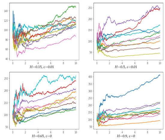
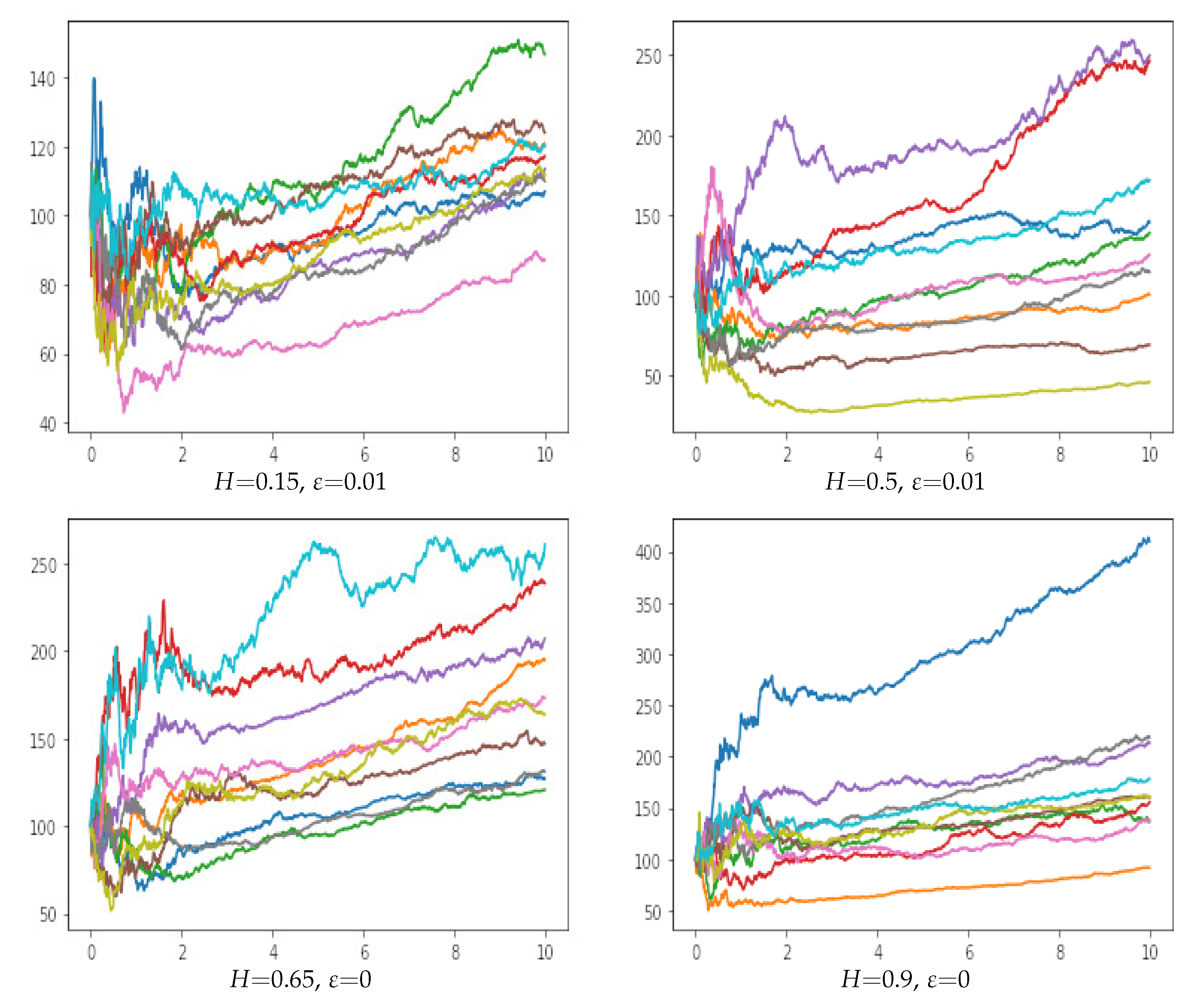
As an illustrative example, the following figures represent 10 sample paths of the stock price process on the interval $[0,T]$ with $N=1000,\rho =0.6,X_0=100,\eta =r=0.05,\nu =0.1,\sigma \left({\widehat{Y}}_{t_i}\right)=0.8{\widehat{Y}}_{t_i}+0.1$. The drift of the fractional volatility process is defined by

$$f(t,y)=\frac{{\sigma }^2}{2}\left(1-e^{-2\kappa t}\right)+\kappa (c-y^2),t\ge 0,y\ge 0,$$

(60)

with $\kappa =1,c=2$. Referring to remark (2), we will choose $\epsilon =0$ when $H>1/2$, and for $H\le 1/2$, we set $\epsilon =0.01$ as shown in Figure 1 below.

Figure 1. Ten sample paths of stock price process ${\left(S_t\right)}_{t\in [0,10]}$ verifying the discrete approximation of stochastic system (12) given by (57) with Hurst parameters $H=0.15,0.5,0.65,0.9$.

4.2.2. Payoff Function with Volatility Taking the Form of Ornstein–Uhlenbeck and Standard fCIR Processes

To the scheme (57), we associate the discrete approximation of the integral $I_T$ provided below, which will be used in the computation of the expression (55).

$${\widehat{I}}_T={\displaystyle \frac{1}{T\sqrt{1-{\rho }^2}}}{\sum }_{i=0}^N{\displaystyle \frac{1}{\sigma \left({\widehat{Y}}_i\right)}}\Delta {\tilde{V}}_{t_i}$$

(61)

Firstly, we consider the stochastic process ${\left(Z_t\right)}_{t\ge 0}$ defined as a fractional Ornstein–Uhlenbeck process, specifically with $f(t,z)=-\theta z^2,$ where $\theta$ is a positive parameter, $\nu =2$ and $H>1/2$. Under these settings, one may recover the model discussed by Bezborodov et al. [27] with $Y_t=Z_t^2$ instead. In this case, the volatility process may not necessarily be positive almost surely, as it violates the Assumption 1, rendering Theorems 1 and 2 inapplicable. To address this, the volatility function $\sigma \left(y\right)$ is chosen to be strictly positive. In addition, we define the payoff function $h\left(x\right)$ as a combination of European and binary options with the same strike price K and time to maturity T, that is,

$$h\left(S_T\right)={(S_T-K)}_{+}+{\mathbf{1}}_{S_T>K}.$$

(62)

The expression for $L\left(S_T\right)$ can be readily deduced from (56) as follows:

$$L\left(S_T\right)=\frac{(S_T-K{)}^2}{2}+(S_T-K){\mathbf{1}}_{S_T>K}.$$

(63)

The payoff function $h\left(S_T\right)$ and $L\left(S_T\right)$ can be visualised in the Figure 2 below with strike price $K=0.5$.

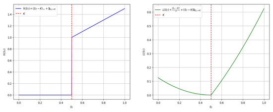
Figure 2. The payoff function $h\left(S_T\right)$ and $L\left(S_T\right)$ with K = 0.5.

Now, to find expected values of the payoff function, we use the same parameters ($\eta =r=0.2,\theta =0.6,T=1$) with different forms of volatility process $\sigma \left(Y_t\right)$ of the infinitesimal log-return process $d{S}_t/S_t$ as in Bezborodov et al. [27]. Since the fCIR process of the form (4) and (5) cannot be used as the drift function $f(t,z)=-\theta z^2<0$ for all $\theta >0$, we consider the direct form of the stochastic volatility ${\left(Y_t\right)}_{t\ge 0}$ that takes the form of the Ornstein–Uhlenbeck process satisfying the following differential equation:

$$d{Y}_t=-\theta Y_{t}dt+\nu d{W}_t^H.$$

In this case, we observe that the values of option prices are not significantly different for $\rho =0$ and $H\ge 1/2$ from Bezborodov et al. [27]. The option prices increase or decrease when $\rho$ is positive or negative, respectively.

Next, consider the fractional volatility process described by a standard fCIR process, that is, with $f(t,z)=\mu -\theta z^2$ and correlation $\rho$ between infinitesimal returns and volatility, the option prices are simulated with $\rho =0.5$ and $\mu =0.1$.

The following tables present the mean prices and their corresponding coefficients of variation for a European–Binary option with the payoff function defined by Equation (62) under different Hurst parameters. The mean values are obtained from an average of ${10}^3$ trials, along with their respective coefficients of variation and option prices are calculated using the expected payoff function discounted by the net present value. We employ two approaches to compute the expectation of the payoff function:

1.

The direct expectation $\mathbb{E}\left[h\left(S_T\right)\right]=\mathbb{E}[{(S_T-K)}_{+}+{\mathbf{1}}_{S_T>K}]$, for a fixed strike price $K=0.5$.

2.

The formula obtained via Malliavin derivative, as given by Equation (55), with $L\left(S_T\right)$ defined by (63).

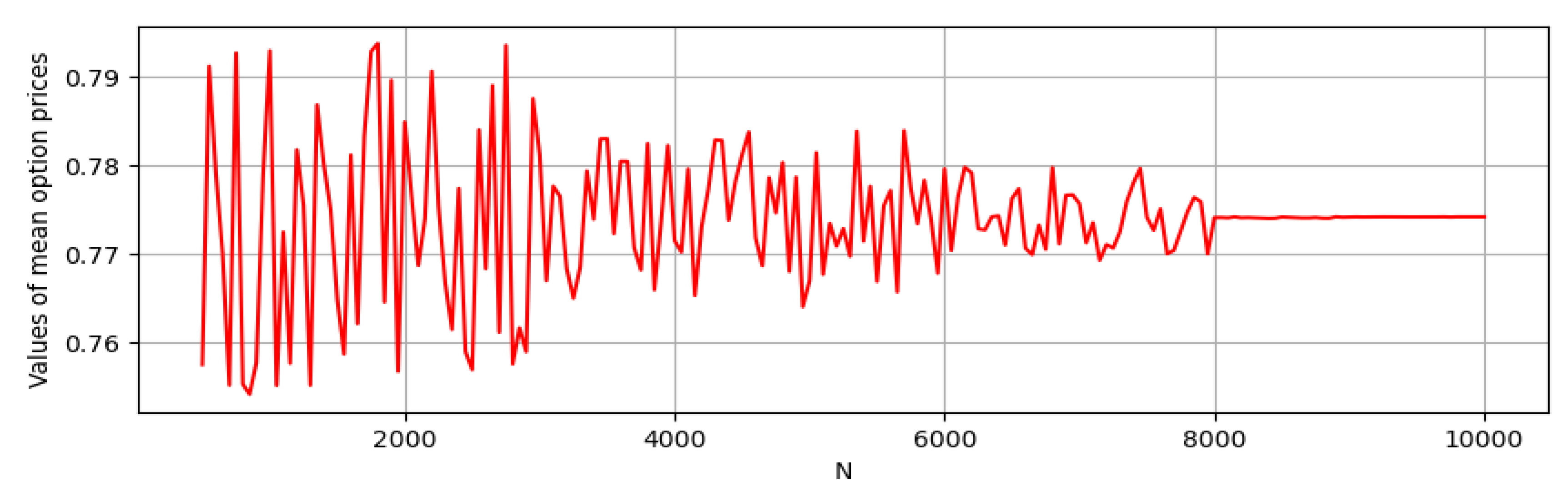
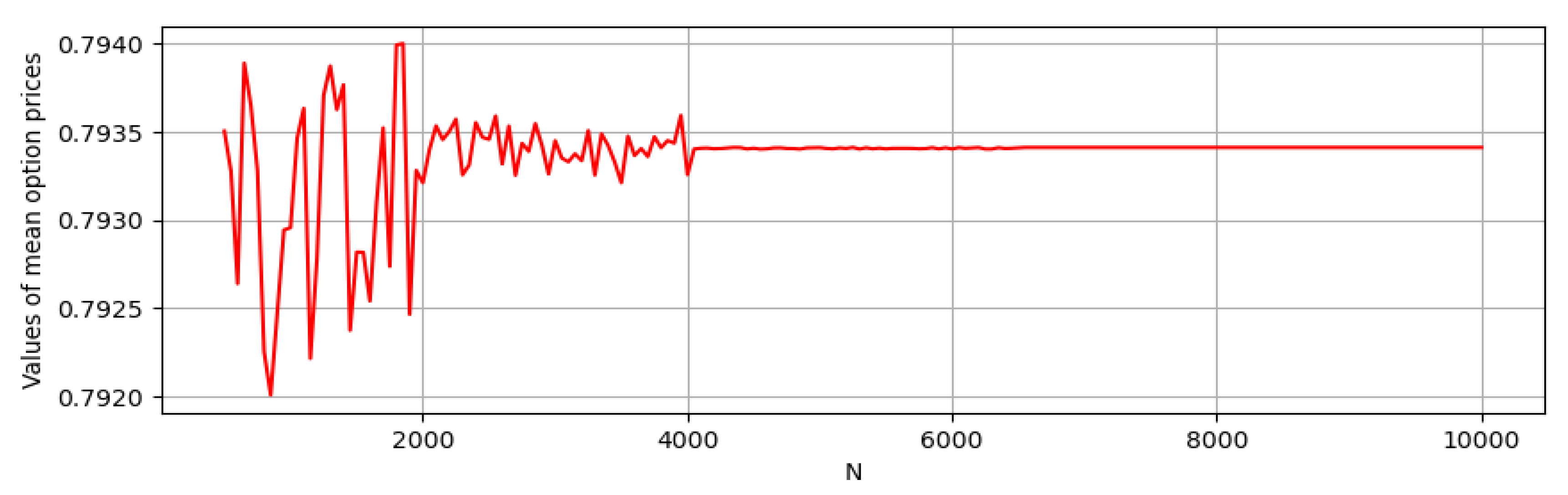
In Table 1, the payoff values at the maturity date T are obtained by performing ${10}^4$ simulations. We observe that the direct estimation of expected values tends to stabilize starting from $N=8000$ (where N represents the number of steps between 0 and T). For example, with $H=0.1$ and $\sigma \left(Y_t\right)=\sqrt{Y_t+0.1}$, the expected values for different values of N are represented in Figure 3.

Table 1. Option prices under direct estimations.

H	0.1		0.3		0.5		0.7		0.9
Mean/CV	Mean	CV	Mean	CV	Mean	CV	Mean	CV	Mean	CV
$\sigma \left(Y_t\right)=\sqrt{Y_t+0.1}$	0.774185342	0.062159457	0.782211975	0.015363114	0.775305642	0.053605636	0.765667823	0.022561751	0.776062568	0.061121985
$\sigma \left(Y_t\right)=Y_t+0.1$	0.932824188	0.023154477	0.959352477	0.019764205	0.946670803	0.008803027	0.952432308	0.016014640	0.948353316	0.008871172
$\sigma \left(Y_t\right)=\sqrt{Y_t^2+1}$	0.707885444	0.093317545	0.715438258	0.077237936	0.695277007	0.053520175	0.720631067	0.041407711	0.729078909	0.085659766

Figure 3. Values of mean option prices for different N under direct estimations.

In Table 2 below, we perform simulations again, this time using the expressions (55), (62), and (63).

Table 2. Option prices using Formula (55).

H	0.1		0.3		0.5		0.7		0.9
Mean/CV	Mean	CV	Mean	CV	Mean	CV	Mean	CV	Mean	CV
$\sigma \left(Y_t\right)=\sqrt{Y_t+0.1}$	0.79340973	0.07560649	0.81121348	0.04028921	0.78827183	0.11421244	0.76642501	0.08935762	0.7704734	0.13411309
$\sigma \left(Y_t\right)=Y_t+0.1$	0.99910672	0.09628926	0.95410606	0.16524115	0.97622451	0.06896021	0.97074148	0.10076119	1.013755924	0.10492516
$\sigma \left(Y_t\right)=\sqrt{Y_t^2+1}$	0.67871381	0.08759139	0.69286223	0.09071164	0.66834204	0.10850252	0.69416225	0.09554705	0.707316469	0.07008638

We may observe that the expected option values are slightly different from those in the previous table. However, the following table demonstrates that the values of the expected payoff function stabilize starting from $N=4000$. One of the main reasons attributed to these satisfactory observations is that the expression of the expectation (55) includes a continuous functional of the stock price process ${\left(S_t\right)}_{t\in [0,T]}$ along with a weight term $(1+I_T)$ that is independent of the functional. This property is even more efficient for discontinuous payoff functions $h\left(S_T\right)$. As in the previous example, choose the Hurst $H=0.1$ and the volatility function $\sigma \left(Y_t\right)=\sqrt{Y_t+0.1}$, the expected values for different values of N under the formula (55) are represented in Figure 4.

Figure 4. Values of mean option prices for different N through Formula (55).

4.2.3. Expected Payoff Function with Volatility Taking the Form of fCIR Process with Time-Varying Parameters

In this section, we perform some simulations of option prices under the fractional Heston model with time-varying parameters. For this, the drift function is given by $f(t,z)=({\mu }_t-{\theta }_t{z}^2)$, where ${\theta }_t=\theta >0$ and ${\mu }_t=c+\frac{{\nu }^2}{2\theta }\left(1-e^{-2\theta t}\right)$. It follows that

$$f(t,z)=\frac{{\nu }^2}{2\theta }\left(1-e^{-2\theta t}\right)+(c-\theta z^2).$$

We shall use $Z_0=1,\nu =0.4,c=0.02,\theta =1$. To keep positiveness of the stochastic process ${\left(Z_t\right)}_{t\ge 0}$ for all $H\in (0,1)$, we shall rather use its approximated stochastic process ${\left(Z_t^{\epsilon }\right)}_{t,\epsilon \ge 0}$ defined by (14), that is

$$d{Z}_t^{\epsilon }=\frac{1}{2}f(t,Z_t^{\epsilon }){\Lambda }_{\epsilon }\left(Z_t^{\epsilon }\right)dt+\frac{\sigma }{2}d{W}_t^H,Z_0^{\epsilon }=Z_0>0,$$

where the function ${\Lambda }_{\epsilon }\left(z\right)$ is defined by

$${\Lambda }_{\epsilon }\left(z\right)={(z{\mathbf{1}}_{\{z>0\}}+\epsilon )}^{-1}$$

with $\epsilon =0.01$ for $H\le 1/2$ and $\epsilon =0$ for $H>1/2$. As previously stated, the fBm is simulated by using the formula (58) and (59). We perform again ${10}^3$ trials for ${10}^4$ simulations and various time-steps on the time interval $[0,1]$. We get the mean of option prices with their corresponding coefficient of variations for different volatility functions $\sigma \left(y\right)$ under the European–Binary option as given in Table 3 for direct estimations and in Table 4 by using (55).

Table 3. Option prices using direct estimations.

H	0.1		0.3		0.5		0.7		0.9
Mean/CV	Mean	CV	Mean	CV	Mean	CV	Mean	CV	Mean	CV
$\sigma \left(Y_t\right)=\sqrt{Y_t+0.1}$	0.757738549	0.048177774	0.769114549	0.057692257	0.756162793	0.045562288	0.756665572	0.051234111	0.763148888	0.043265712
$\sigma \left(Y_t\right)=Y_t+0.1$	0.932035897	0.012595508	0.934337494	0.022642941	0.933212125	0.024487	0.928706032	0.014969569	0.929103212	0.01457107
$\sigma \left(Y_t\right)=\sqrt{Y_t^2+1}$	0.770104152	0.088196662	0.782432528	0.062946479	0.75433847	0.069371091	0.746931996	0.072156192	0.75975843	0.084981952

Table 4. Option prices using (55).

H	0.1		0.3		0.5		0.7		0.9
Mean/CV	Mean	CV	Mean	CV	Mean	CV	Mean	CV	Mean	CV
$\sigma \left(Y_t\right)=\sqrt{Y_t+0.1}$	0.769174923	0.159481951	0.79459017	0.136648616	0.781942914	0.157116756	0.747618003	0.12525256	0.755713234	0.06592363
$\sigma \left(Y_t\right)=Y_t+0.1$	0.94650013	0.102404072	1.02769617	0.128530355	0.919334248	0.111971197	0.983793301	0.095406694	0.88152163	0.101523439
$\sigma \left(Y_t\right)=\sqrt{Y_t^2+1}$	0.803170587	0.273211512	0.793796973	0.205160841	0.756164588	0.210899491	0.742696383	0.203031148	0.759959966	0.198280955

Note that observations from the previous sections also apply to this one.

5. Conclusions

In this paper, we have constructed the fractional Heston-type model as a stochastic system comprising the stock price process ${\left(S_t\right)}_{t\ge 0}$ modeled by a geometric Brownian motion. The volatility of this process is represented as a strictly positive and Lipschitz continuous function $\sigma \left(Y_t\right)$ of fractional Cox–Ingersoll–Ross process ${\left(Y_t\right)}_{t\ge 0}$, which is characterized by the square of a stochastic process ${\left(Z_t\right)}_{t\ge 0}$ that satisfies a stochastic differential equation with additive fractional Brownian motion.

To ensure the positivity of the stochastic process ${\left(Z_t\right)}_{t\ge 0}$ for all Hurst parameters $H\in (0,1)$, we have considered an approximating sequence ${\left(Z_t^{\epsilon }\right)}_{t\ge 0,,\epsilon >0}$ converging to ${\left(Z_t\right)}_{t\ge 0}$ in $L^p(\Omega )$ for all $p\ge 1$. This construction also enables us to demonstrate that ${\left(Z_t\right)}_{t\ge 0}$, ${\left(S_t\right)}_{t\ge 0}$, and the payoff function $h\left(S_t\right)$ are Malliavin differentiable. Furthermore, we establish that the law of the stochastic processes ${\left(Z_t\right)}_{t\ge 0}$ and ${\left(S_t\right)}_{t\ge 0}$ is absolutely continuous with respect to the Lebesgue measure over any finite interval $[0,t]$.

To support our findings, we conducted simulations. Firstly, we modeled volatility using the Ornstein–Uhlenbeck process, corroborating the results found in Bezborodov et al. [27]. Secondly, we explored the fractional Cox–Ingersoll–Ross process with time-varying parameters. Our observations indicate that option prices exhibit greater stability under the expected value of option prices obtained through Malliavin calculus.

References

- Heston, S.L. A closed-form solution for options with stochastic volatility with applications to bond and currency options. Rev. Financ. Stud. 1993, 6, 327–343. [Google Scholar] [CrossRef]
- Alòs, E.; Mancino, M.E.; Wang, T.H. Volatility and volatility-linked derivatives: Estimation, modeling, and pricing. Decis. Econ. Financ. 2019, 42, 321–349. [Google Scholar] [CrossRef]
- Alos, E.; León, J.A.; Vives, J. On the short-time behavior of the implied volatility for jump-diffusion models with stochastic volatility. Financ. Stochastics 2007, 11, 571–589. [Google Scholar] [CrossRef]
- Fukasawa, M. Asymptotic analysis for stochastic volatility: Martingale expansion. Financ. Stochastics 2011, 15, 635–654. [Google Scholar] [CrossRef]
- Gatheral, J.; Jaisson, T.; Rosenbaum, M. Volatility is rough. Quant. Financ. 2018, 18, 933–949. [Google Scholar] [CrossRef]
- Livieri, G.; Mouti, S.; Pallavicini, A.; Rosenbaum, M. Rough volatility: Evidence from option prices. Iise Trans. 2018, 50, 767–776. [Google Scholar] [CrossRef]
- Takaishi, T. Rough volatility of Bitcoin. Financ. Res. Lett. 2020, 32, 101379. [Google Scholar] [CrossRef]
- Fukasawa, M. Volatility has to be rough. Quant. Financ. 2021, 21, 1–8. [Google Scholar] [CrossRef]
- Brandi, G.; Di Matteo, T. Multiscaling and rough volatility: An empirical investigation. Int. Rev. Financ. Anal. 2022, 84, 102324. [Google Scholar] [CrossRef]
- Comte, F.; Renault, E. Long memory in continuous-time stochastic volatility models. Math. Financ. 1998, 8, 291–323. [Google Scholar] [CrossRef]
- Chronopoulou, A.; Viens, F.G. Hurst index estimation for self-similar processes with long-memory. In Recent Development in Stochastic Dynamics and Stochastic Analysis; World Scientific: Singapore, 2010; pp. 91–117. [Google Scholar]
- Chronopoulou, A.; Viens, F.G. Estimation and pricing under long-memory stochastic volatility. Ann. Financ. 2012, 8, 379–403. [Google Scholar] [CrossRef]
- Tripathy, N. Long memory and volatility persistence across BRICS stock markets. Res. Int. Bus. Financ. 2022, 63, 101782. [Google Scholar] [CrossRef]
- Alòs, E.; Lorite, D.G. Malliavin Calculus in Finance: Theory and Practice; Chapman and Hall/CRC: Boca Raton, FL, USA, 2021. [Google Scholar]
- Funahashi, H.; Kijima, M. A solution to the time-scale fractional puzzle in the implied volatility. Fractal Fract. 2017, 1, 14. [Google Scholar] [CrossRef]
- Alòs, E.; Yang, Y. A fractional Heston model with H>1/2. Stochastics 2017, 89, 384–399. [Google Scholar] [CrossRef]
- Mishura, Y.; Yurchenko-Tytarenko, A. Approximating Expected Value of an Option with Non-Lipschitz Payoff in Fractional Heston-Type Model. Int. J. Theor. Appl. Financ. 2020, 23, 2050031. [Google Scholar] [CrossRef]
- Mehrdoust, F.; Fallah, S. On the calibration of fractional two-factor stochastic volatility model with non-Lipschitz diffusions. Commun. -Stat.-Simul. Comput. 2022, 51, 6332–6351. [Google Scholar] [CrossRef]
- Tong, K.Z.; Liu, A. The valuation of barrier options under a threshold rough Heston model. J. Manag. Sci. Eng. 2023, 8, 15–31. [Google Scholar] [CrossRef]
- Richard, A.; Tan, X.; Yang, F. On the discrete-time simulation of the rough Heston model. Siam J. Financ. Math. 2023, 14, 223–249. [Google Scholar] [CrossRef]
- Mishura, Y.; Piterbarg, V.; Ralchenko, K.; Yurchenko-Tytarenko, A. Stochastic representation and path properties of a fractional Cox–Ingersoll–Ross process. Theory Probab. Math. Stat. 2018, 97, 167–182. [Google Scholar] [CrossRef]
- Mishura, Y.; Yurchenko-Tytarenko, A. Fractional Cox–Ingersoll–Ross process with non-zero “mean”. Mod. Stochastics Theory Appl. 2018, 5, 99–111. [Google Scholar] [CrossRef]
- Mpanda, M.M.; Mukeru, S.; Mulaudzi, M. Generalisation of fractional Cox–Ingersoll–Ross process. Results Appl. Math. 2022, 15, 100322. [Google Scholar] [CrossRef]
- Nourdin, I. Selected Aspects of Fractional Brownian Motion; Springer: Berlin/Heidelberg, Germany, 2012; Volume 4. [Google Scholar]
- Decreusefond, L.; Üstünel, A.S. Stochastic analysis of the fractional Brownian motion. Potential Anal. 1999, 10, 177–214. [Google Scholar] [CrossRef]
- Nualart, D.; Ouknine, Y. Regularization of differential equations by fractional noise. Stoch. Processes Their Appl. 2002, 102, 103–116. [Google Scholar] [CrossRef]
- Bezborodov, V.; Di Persio, L.; Mishura, Y. Option pricing with fractional stochastic volatility and discontinuous payoff function of polynomial growth. Methodol. Comput. Appl. Probab. 2019, 21, 331–366. [Google Scholar] [CrossRef]
- Alos, E.; Ewald, C.O. Malliavin differentiability of the Heston volatility and applications to option pricing. Adv. Appl. Probab. 2008, 40, 144–162. [Google Scholar] [CrossRef]
- Hu, Y.; Nualart, D.; Song, X. A singular stochastic differential equation driven by fractional Brownian motion. Stat. Probab. Lett. 2008, 78, 2075–2085. [Google Scholar] [CrossRef]
- Mishura, Y.; Yurchenko-Tytarenko, A. Fractional Cox–Ingersoll–Ross process with small Hurst indices. Mod. Stochastics Theory Appl. 2019, 6, 13–39. [Google Scholar] [CrossRef]
- Nualart, D. The Malliavin Calculus and Related Topics; Springer: Berlin/Heidelberg, Germany, 2006; Volume 1995. [Google Scholar]
- Da Prato, G. Introduction to Stochastic Analysis and Malliavin Calculus; Springer: Berlin/Heidelberg, Germany, 2014; Volume 13. [Google Scholar]
- Nunno, G.D.; Øksendal, B.; Proske, F. Malliavin Calculus for Lévy Processes with Applications to Finance; Springer: Berlin/Heidelberg, Germany, 2008. [Google Scholar]
- Bouleau, N.; Hirsch, F. Dirichlet Forms and Analysis on Wiener Space; Walter de Gruyter: Berlin, Germany, 2010; Volume 14. [Google Scholar]
- Detemple, J.; Garcia, R.; Rindisbacher, M. Representation formulas for Malliavin derivatives of diffusion processes. Financ. Stochastics 2005, 9, 349–367. [Google Scholar] [CrossRef]
- Mukeru, S. The zero set of fractional Brownian motion is a Salem set. J. Fourier Anal. Appl. 2018, 24, 957–999. [Google Scholar] [CrossRef]
- Altmayer, M.; Neuenkirch, A. Multilevel Monte Carlo quadrature of discontinuous payoffs in the generalized Heston model using Malliavin integration by parts. Siam J. Financ. Math. 2015, 6, 22–52. [Google Scholar] [CrossRef]
Disclaimer/Publisher’s Note: The statements, opinions and data contained in all publications are solely those of the individual author(s) and contributor(s) and not of MDPI and/or the editor(s). MDPI and/or the editor(s) disclaim responsibility for any injury to people or property resulting from any ideas, methods, instructions or products referred to in the content. |
© 2024 by the author. Licensee MDPI, Basel, Switzerland. This article is an open access article distributed under the terms and conditions of the Creative Commons Attribution (CC BY) license (https://creativecommons.org/licenses/by/4.0/).