Reduced Order Modeling of System by Dynamic Modal Decom-Position with Fractal Dimension Feature Embedding

Abstract

The balance between accuracy and computational complexity is currently a focal point of research in dynamical system modeling. From the perspective of model reduction, this paper addresses the mode selection strategy in Dynamic Mode Decomposition (DMD) by integrating an embedded fractal theory based on fractal dimension (FD). The existing model selection methods lack interpretability and exhibit arbitrariness in choosing mode dimension truncation levels. To address these issues, this paper analyzes the geometric features of modes for the dimensional characteristics of dynamical systems. By calculating the box counting dimension (BCD) of modes and the correlation dimension (CD) and embedding dimension (ED) of the original dynamical system, it achieves guidance on the importance ranking of modes and the truncation order of modes in DMD. To validate the practicality of this method, it is applied to the reduction applications on the reconstruction of the velocity field of cylinder wake flow and the force field of compressor blades. Theoretical results demonstrate that the proposed selection technique can effectively characterize the primary dynamic features of the original dynamical systems. By employing a loss function to measure the accuracy of the reconstruction models, the computed results show that the overall errors of the reconstruction models are below 5%. These results indicate that this method, based on fractal theory, ensures the model’s accuracy and significantly reduces the complexity of subsequent computations, exhibiting strong interpretability and practicality.

1. Introduction

In engineering applications such as turbomachines, the dynamics model is often characterized by high-dimensional or infinite-dimensional nonlinearities [1]. Direct solutions for these highly coupled systems encounter challenges related to convergence and computational time, and it is difficult to analyze using analytical methods. At present, the dimensionality reduction of such a system is a bottleneck in the study of nonlinear dynamics. The commonly used dimension reduction methods, such as the nonlinear Galerkin method and principal component analysis (PCA), are only applicable to some special dynamical systems. Therefore, in the field of nonlinear dynamics research, it is crucial to seek an effective dimensionality reduction method to reduce the high-dimensional complex nonlinear system to a low-dimensional system with only a few degrees of freedom. This is also the focus of the current research.

Scholars in the field of aeroelasticity, such as Dowell [2] and Silva [3], proposed to construct a reduced order model (ROM) for unsteady flow. A ROM is a low-order mathematical model derived from the approximate projection of a full-order model. The purpose of constructing a ROM is twofold: firstly, to offer a mathematical description of the primary dynamics with reduced order and computation cost; secondly, to serve as a tool to analyze the dynamic characteristics of the system. ROM can describe the main dynamics of the original system with relatively few degrees of freedom. Moreover, it reduces computational burden while preserving credibility and high fidelity.

Two main types of ROMs are commonly applied. One involves extracting features from input and output data. The other involves extracting features to achieve modeling reduction. System identification entails analyzing the input and output data to determine a function that closely represents the original system. It can enable the fitting of the dynamic or static characteristics of the actual system. Currently, there are various reduced order models for nonlinear aerodynamic system identification, such as the Volterra model, time series ARMA model, and neural networks.

The algorithm for flow feature extraction involves searching for low-dimensional subspaces to represent high-dimensional systems through the superposition. The entire system is projected onto the subspace formed by the extracted modes, allowing for the description of flow evolution in a low dimensional space. Methods for feature extraction mainly include two categories: Proper Orthogonal Decomposition (POD) and Dynamic Mode Decomposition (DMD). Similar to PCA and Singular Value Decomposition (SVD), the POD aims to project high-order, nonlinear systems onto a lower dimensional state space through orthogonal modal projections while minimizing mapping errors.

The DMD algorithm treats the system as linearity within a specified timestep. Based on the principle of matrix decomposition, DMD utilizes the data from adjacent time instances to decompose into a set of modes and temporal evolution [4]. In contrast to the POD, the DMD decomposes high-dimensional systems into a weighted sum of spatial modes and corresponding temporal dynamics. This decomposition results in the modal components possessing a singular frequency and growth rate. This advantage of DMD is reflected for obtaining modal features and dynamic information simultaneously. This distinction provides a unique benefit in spatio-temporal coupled modeling.

Through dynamic decomposition, Gao [5] successfully predicted the stability of excavation settlement. Chen [6] effectively reconstructed sea surface temperature data at the mouth of the Yangtze River by DMD, addressing the sampling issue in dynamic systems. In recent years, the applications of the DMD in fluid mechanics have become increasingly widespread. A key problem in the process of decomposing the flow field is how to capture the flow characteristics in the most simplified structure. In DMD, the essence of these issues lies in mode selection. The aim is to obtain an accurate representation of the system for optimal estimation by minimizing the number of modes. This involves two main problems: the sorting method and the truncation method of DMD modes. In contrast to the POD, which directly sorts modes based on energy information, the sorting method for DMD is not unique. Therefore, it is necessary to use reasonable means to select the most important modes.

Rowley [7] implemented modal sorting based on the norms of each mode. Schmid [8] defined modal amplitude by projecting the data sequence onto the modes with the coefficients indicating the importance. The modal amplitude was defined by the projection of the first snapshot onto the DMD modes [9]. This measure was used to extract the structure of the turbulent boundary layer, with the amplitude representing the contribution of each mode to the initial field. A two-step modal selection process was performed by Jovanović [10], which defined amplitude according to the contribution of modes to the reduced-dimensional snapshot. Building upon Rowley’s approach, an improvement was suggested by weighting the modal norm with the magnitude of DMD eigenvalues. Thereby, a new objective function to eliminate large norms was constructed [11]. This criterion reflects the contribution of each mode, with its accuracy surpassing the criteria based on modal norms.

Furthermore, Tissot [12] proposed a criterion based on the contribution of time-averaged modal energy. It considered the overall contribution of modes within a sample segment and provided a global understanding of modal energy. In the parameterized DMD proposed by Sayadi [13], a sparse structure was obtained using the method of sparse-enhanced DMD. The amplitudes of each mode were redefined as modal time coefficients. They can be integrated over time to achieve data extrapolation. Compared to standard DMD with fixed amplitudes over time, this algorithm can identify the main dynamic modes based on the temporal evolution process. By considering a combination of several physical characteristics of the modes, a new selection criterion was proposed based on an energy definition formula [14]. It was considered to address the limitation of previous selection methods of transient energy modes. Considering the interaction of different modes, Krake [15] proposed modal selection criteria with distance and harmonic cluster.

The above-mentioned methods rely on traditional modal parameters: amplitudes, modal eigenvalues, and modal paradigms. However, they ignore the physical characteristics and detailed information of the system. Moreover, the lack of clear guidelines for modal interception makes the methods for intercepting modes with the loss function [10,14] rather arbitrary. And this arbitrariness leads to a lack of interpretability. The fractal dimension is a quantitative parameter used to characterize the degree of irregularity of complex systems. Box counting dimension (BCD) and correlation dimension (CD) are representative fractal characterizations of the fractal dimension. BCD is commonly used for dimension measurement of static geometries by counting the dimensionality by means of a box cover. CD is applied to describe chaotic behavior in dynamical systems. It measures the correlation between the state points in a system, which can reflect the diffusion degree of the system in phase space.

The key challenge regarding the reduction of the aerodynamic system is the mode selection, which effectively represents the high-dimension unsteady flow through the superposition of low-dimension subspaces. To address this need, a novel approach that incorporates modal morphological features and fractal theory is brought up, taking a mathematical perspective on the selection of DMD modes. The innovations are as follows:

• System Fractal Feature Description. By employing BCD and CD for fractal features of dynamical systems, it provides a new perspective on nonlinear system analysis. The complex structure of modes can be better captured by fractal characterization. Then, it is possible to gain a deeper understanding of the variability of the different modes, and thus select key modes more effectively for system modeling.
• Modal Selection Strategy. Fractal features provide information about the dynamic properties of the prime system, which can guide the selection of the most representative modes for the dynamic behavior of the system. By combining fractal characterization with DMD modal selection, the dynamic behavior of system can be captured more accurately. The credibility and predictive power of the model can be improved.

This paper analyzes the mode extraction with DMD from the perspective of fractal structures, aiming to identify the primary modes that are the most representative of the original dynamical system through fractal characteristics. The main research contents can be described in the following chapters. Firstly, a detailed introduction to fractal theory is presented in the methodology. Based on the mode selection strategy using BCD and CD, the applications of circular cylinder vortex and aerodynamic force on the blade are dynamically decomposed for the examination of the feasibility of the method, subsequently. Finally, the loss function is chosen as the evaluation index to verify reliability and accuracy with the other method. It is indicated that compared with sparsity-promoting DMD, this novel fractal dimension estimation method reflects the fractal characteristics of the dynamic system after modal decomposition well. The reduction approach is promoted by the specified mode selection strategy of fractal dimension embedding.

2. Methodology of Fractal and Dynamic Modal Decomposition Algorithms

2.1. Fractal Dimension Theory

Fractal is a geometric representation of natural phenomena. It struggles to capture characteristics such as nonlinearity, multiscale, and self-similarity for traditional analysis. The property of fractal dimension is to provide a relative measure of the number of basic building blocks that form a pattern [16]. Thus, the FD can describe the spatial structure of a system at different scales. It can reveal a quantitative description of the spatial distribution and spatial correlation of a system, providing a path for understanding and modeling the complex system.

2.1.1. Definition of Box Counting Dimension

The BCD reflects the complexity and fractal characteristics of the dataset [16]. For any $r>0$, $N_r(A)$ denotes the minimum number of n-dimensional boxes with edge length r used to cover subset A. If there exists a d, when $r\to 0$ there is

$$N_r(A)\propto \frac{1}{r^d},$$

(1)

then $d$ is set to be the box counting dimension of A.

Divide the space containing set A into grids with side length r, and then find the minimum number of grids. By taking different values of $r_i$, a series of corresponding $N_{r_i}(A)$ can be obtained. Using the formula

$$d=-\underset{r\to 0}{\lim }\frac{\log N_r(A)}{\log r},$$

(2)

the d as BCD of set A can be determined. However, in practical calculations, r cannot be valued infinitely small. Usually, a graph is plotted with $-\log r$ as the x-axis and $\log N_r(A)$ as the y-axis. Linear regression is performed to obtain the slope of the line, which is represented by the BCD.

This article primarily focuses on two types of calculation: the 2D image BCD and the fixed radius BCD. The 2D image BCD is first converted to black and white and then divided into grids for calculation of the BCD parameter d. For the fixed radius BCD determination, the center of study area is used as the center of a circle, and circles of varying radii are drawn. The number of points contained within each circle is then counted, and the parameter d is determined by changing the value of r sequentially.

2.1.2. Definition of Correlation Dimension

CD is sensitive to the temporal behavior of a system and can effectively capture the dynamic properties of nonlinear systems. In the beginning of the approach, it is necessary to reconstruct the phase space of the time series, resulting in a set of points $\left\{X_i\right\}(i=1,\dots ,N)$, estimating the distance between any two points subsequently. When this distance is less than a given number r, the two points are considered to be associated. If we calculate the proportion of the associated point pairs, then the definition of the correlation integral is set as follows:

$$C(r)=\frac{1}{N(N-1)}{\displaystyle \sum _{i\ne j}[H(r-\left|\right|X_i-X_j\left|\right|)]}.$$

(3)

The correlation integral reflects the probability of the distribution of the distance between two points less than r on the attractor in the phase space. Therefore, for the parameter d of the correlation dimension, it is shown as follows:

$$\underset{r\to 0}{\lim }C(r)\propto r^d,$$

(4)

$$d=\underset{r\to 0}{\lim }\frac{d\ln C(r)}{d\ln r}.$$

(5)

In the actual calculation process, $\ln C(r)$ is plotted as the vertical coordinate and $\ln r$ as the horizontal coordinate. If we take the linear regression in obvious part of the linearity, the slope of the line is indicated as the correlation dimension.

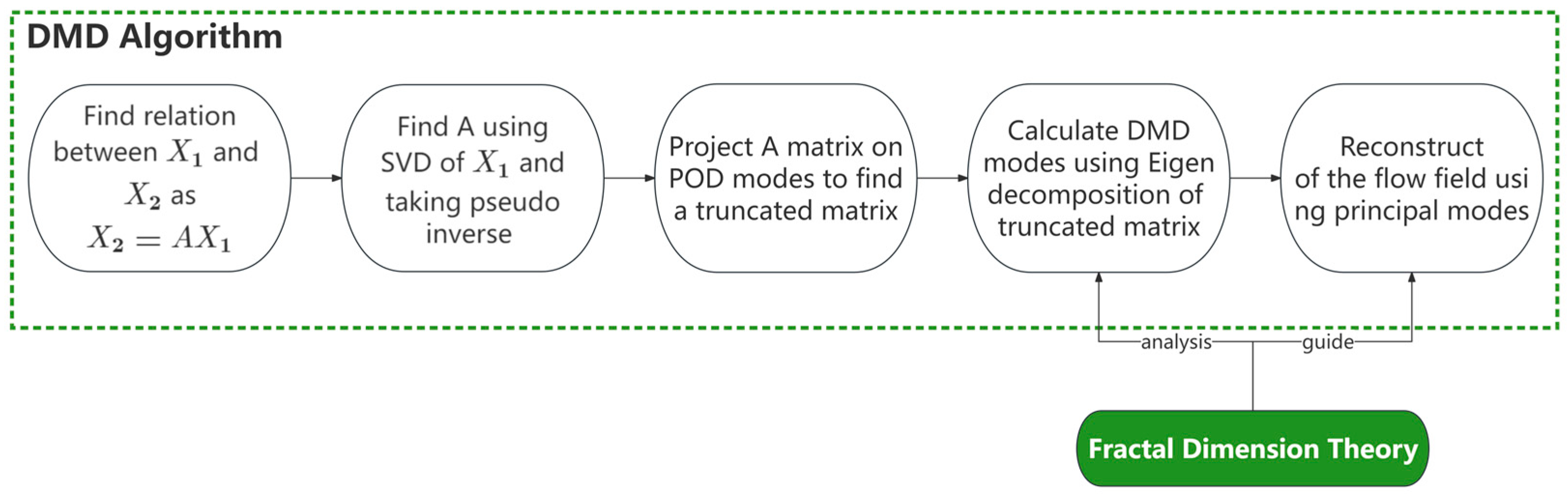
2.2. Dynamic Modal Decomposition Theory

We set the snapshot flow field data of N different moments in a matrix form according to the time series

$$S_1^N=[x_1,x_2,\dots ,x_N],$$

(6)

where $x_i={[x_{i1},x_{i2},\dots ,x_{iM}]}^T$ is the snapshot of the flow field at the $i$-th moment, and we let $\Delta t$ be the neighboring snapshot time interval.

We let the system matrix A satisfy the following conditions:

$$x_{i+1}=A{x}_i,i=1,2,\dots ,N-1.$$

(7)

This means the system matrix A remains constant in the time dimension.

Therefore, it can be concluded that the relationship between $S_1^{N-1}=[x_1,x_2,\dots ,x_{N-1}]$ and $S_2^N=[x_2,x_3,\dots ,x_N]$ is equal with

$$S_2^N=A{S}_1^{N-1}.$$

(8)

We compute the SVD of $S_1^{N-1}$ as

$$S_1^{N-1}=U\Sigma V\prime ,U\in C^{M\times r},V\in C^{(N-1)\times r}.$$

(9)

where matrix $\Sigma$ is the $r\times r$ diagonal matrix. Through a similarity transformation, the expression for A is projected on to the $r$ POD modes as follows:

$$A=U\tilde{A}U\prime ,UU\prime =I,VV\prime =I,$$

(10)

where “$\prime$“ denotes the complex conjugate transpose. The matrices U and V contain information about the spatial structure of the original system and the time evolution in the system.

Then, the matrix $\tilde{A}$ is determined by transforming into a Frobenius minimization,

$$\underset{A}{\min }||S_2^N-A{S}_1^{N-1}{\left|\right|}_F^2=\underset{\tilde{A}}{\min }||S_2^N-U\tilde{A}\Sigma V\prime {\left|\right|}_F^2.$$

(11)

Therefore, the approximate matrix $\tilde{A}$ can be deduced as follows:

$$A\approx \tilde{A}=U\prime S_2^{N}V{\Sigma }^{-1},$$

(12)

where the approximate matrix $\tilde{A}$ contains the main eigenvalues of matrix A. With setting i-th eigenvalue as ${\mu }_i$ and the corresponding eigenvector as $w_i$, the $i$-th DMD mode is represented by

$${\Phi }_i=U{w}_i.$$

(13)

Therefore, an estimation of i-th snapshot at a given time can be obtained as follows:

$$x_i=A{x}_{i-1}=U\tilde{A}U\prime x_{i-1}=UW\Lambda WU\prime x_{i-1}=UW{\Lambda }^{i-1}{W}^{-1}U\prime x_1=\Phi {\Lambda }^{i-1}{\Phi }^{-1}{x}_1,$$

(14)

where the column vectors of $W$ are the eigenvectors of $\tilde{A}$ and $\Lambda$ is the diagonal matrix whose main diagonal elements are the eigenvalues of $\tilde{A}$. According to the standard DMD method, the amplitude represents the modal contribution to the initial snapshot [17]. The specific equation is given below:

$$\alpha =W^{-1}U\prime x_1={\Phi }^{-1}{x}_1\alpha ={\left[{\alpha }_1,\dots ,{\alpha }_r\right]}^T.$$

(15)

If the flow snapshot of the first timestep is projected onto the modal space as

$$x_1=\Phi \alpha ,$$

(16)

then the expression for the reconstructed flow field can be written as follows:

$$x_i=\Phi {\Lambda }^{i-1}\alpha ={\displaystyle \sum _{j=1}^r{\Phi }_j}{\left({\mu }_j\right)}^{i-1}{\alpha }_j.$$

(17)

The corresponding matrix is formed as follows:

$$S_1^{N-1}=\left[x_1,x_2,x_3,\dots ,x_{N-1}\right]=\Phi \mathrm{diag}(\alpha )V_{and}=\left[{\Phi }_1,{\Phi }_2,\dots ,{\Phi }_r\right]\left[\begin{array}{ccc}{\alpha }_1& & \\ \begin{array}{l}\\ \end{array}& \begin{array}{l}{\alpha }_2\\ \end{array}& \begin{array}{l}\\ \ddots \end{array}\\ & & \end{array}\begin{array}{c}\\ \\ \\ {\alpha }_r\end{array}\right]\left[\begin{array}{lll}1\hfill & {\mu }_1\hfill & \dots \hfill \\ 1\hfill & {\mu }_2\hfill & \dots \hfill \\ ⋮\hfill & ⋮\hfill & \ddots \hfill \\ 1\hfill & {\mu }_r\hfill & \dots \hfill \end{array}\begin{array}{c}{\left({\mu }_1\right)}^{N-2}\\ {\left({\mu }_2\right)}^{N-2}\\ ⋮\\ {\left({\mu }_r\right)}^{N-2}\end{array}\right].$$

(18)

3. Application of Fractal Dimension on Circular Cylinder Vortex

The abbreviated flowchart of system reduction is indicated in Figure 1. In this process, the fractal theory is applied to analyze the ordering of the modes and guides the truncation of the matrices.

3.1. Source of Data

In this section, the vorticity field of a cylindrical wake with a Reynolds number of 100 is selected as an application to validate the effectiveness of the reduction method under fractal dimension analysis. The snapshots of the flow field are adopted from the accompanying data [17]. The flow field of the cylinder consists of four computation domains, each containing 449 × 199 grid points. After the simulation with a timestep of 0.02 s is converged to a stable state of vortex shedding, the snapshots of the flow field are captured at an interval of 10 timesteps. Finally, a total of 150 snapshots are collected in the form of a matrix of 89,351 × 150. Each column represents a snapshot of the flow, while each row represents the temporal evolution of the field. A snapshot of the cylinder wake data is shown in Figure 2.

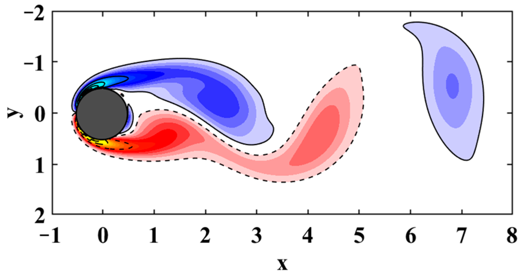
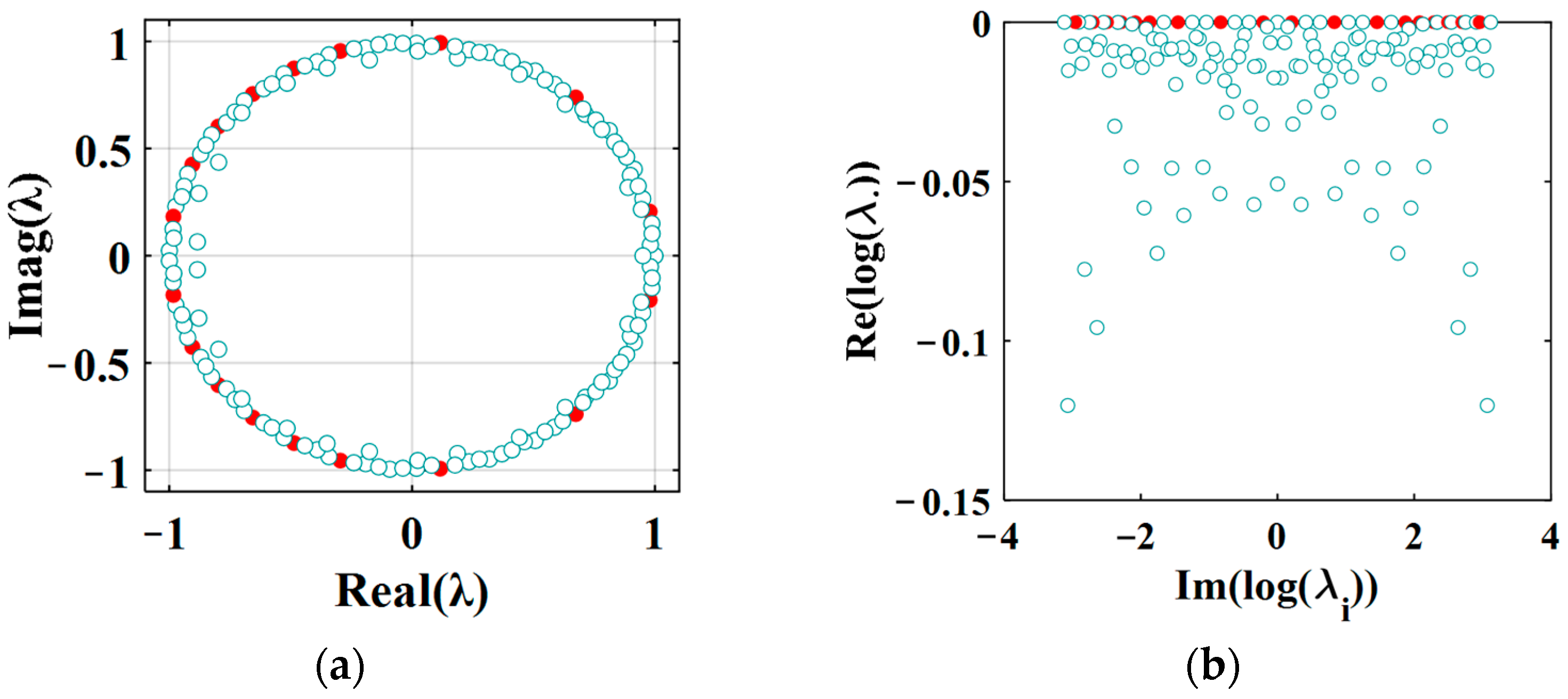
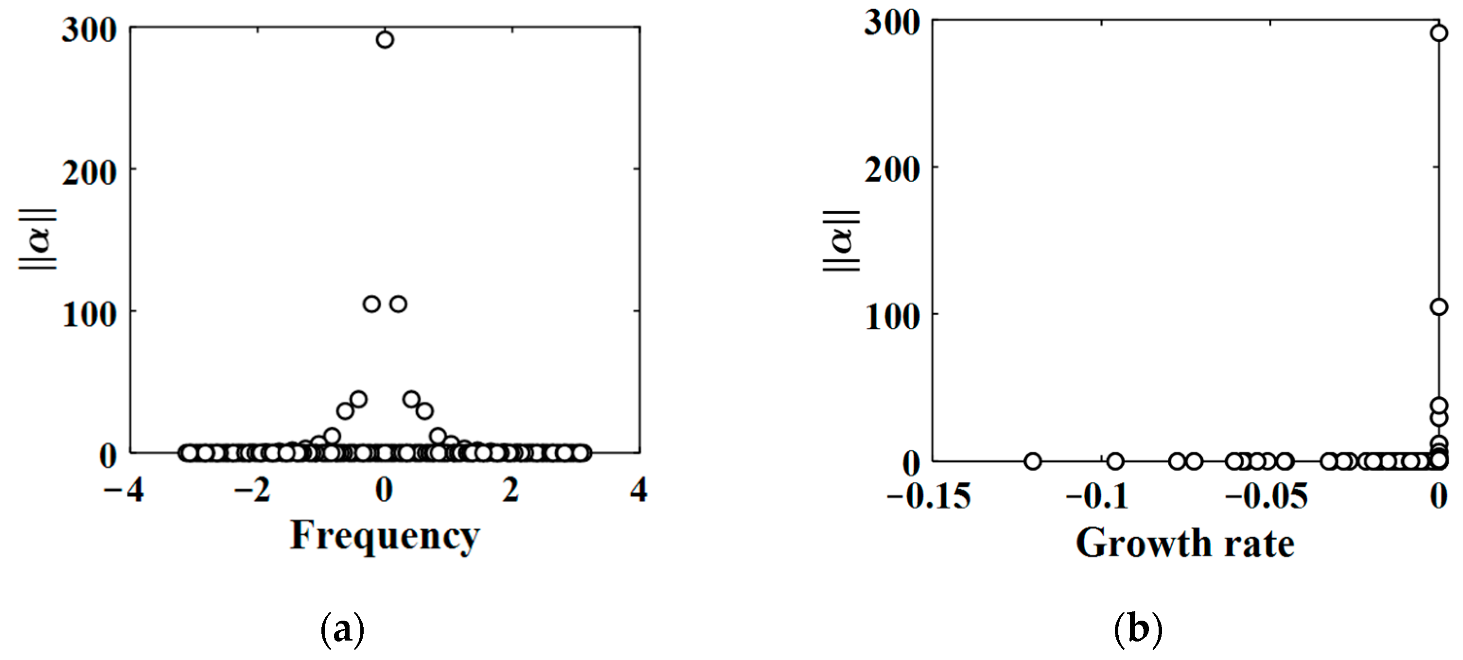
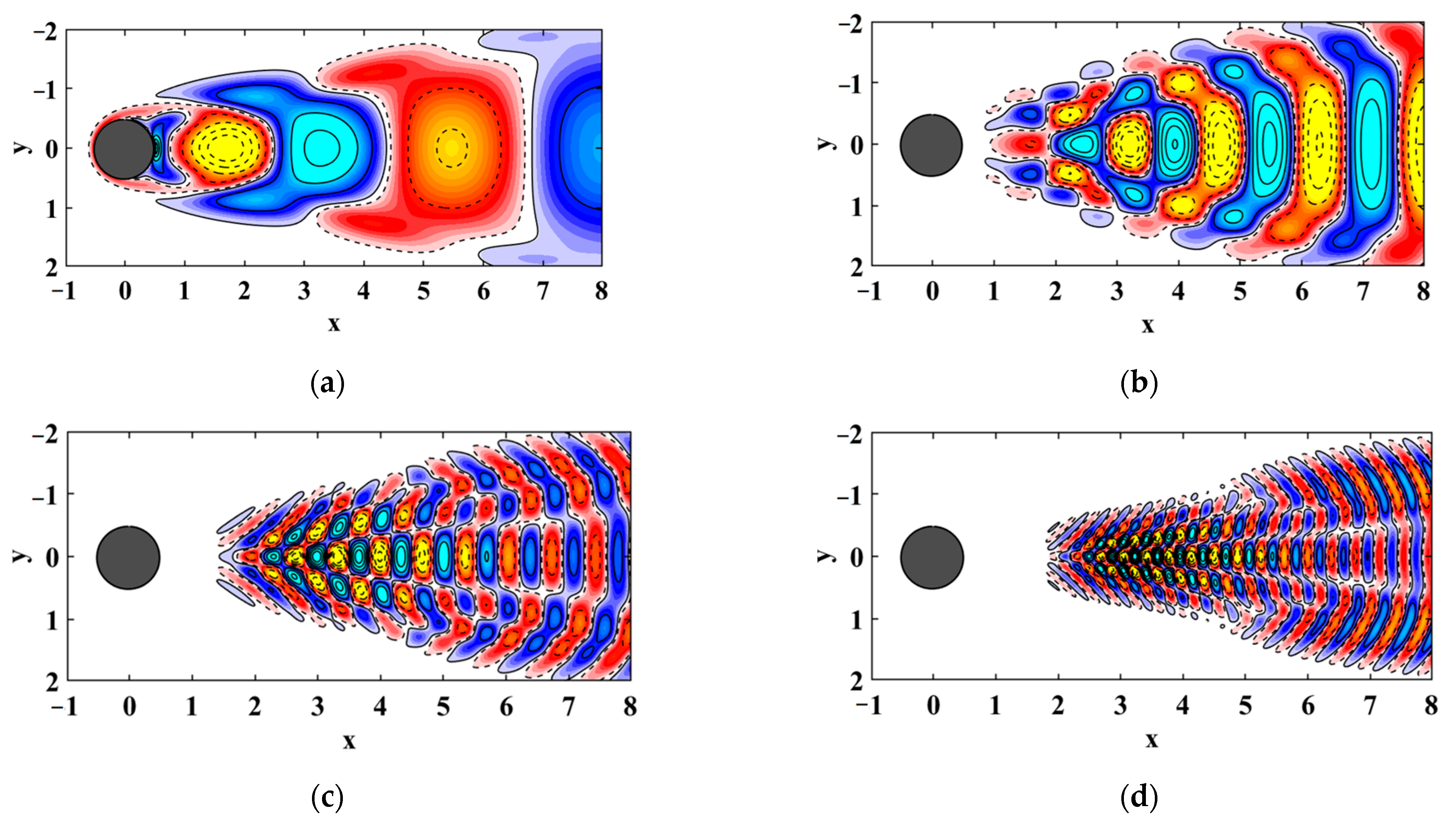
3.2. DMD Analysis of the Cylinder Wake Flow Field

Within the DMD for modal decomposition, it is assumed here that the system at the latter moment of the flow field can be approximated linearly by the flow field at the former moment. First, the flow field samples are subjected to DMD computation for modes ${\Phi }_j$, amplitudes ${\alpha }_j$, and eigenvalues ${\lambda }_j$. Eigenvalues of DMD modes are presented as conjugate complex numbers. The real part of the modal eigenvalue responds to the degree of growth or decay of the mode in the time domain. The imaginary part responds to the frequency of vibration of the mode. The formulas are as follows:

$$g_j=\mathrm{Re}\left\{\lg \left({\lambda }_j\right)\right\}/\Delta t,{\omega }_j=\mathrm{Im}\left\{\lg \left({\lambda }_j\right)\right\}/\Delta t.$$

(19)

Figure 3 shows the distribution of the eigenvalues of the DMD modes of the cylinder wake. In Figure 3a, the horizontal axis represents the real part of the eigenvalue and the vertical axis represents the imaginary part of the eigenvalue. In Figure 3b, the horizontal axis represents the growth of the mode and the vertical axis represents the vibration frequency of the mode. The filled red dots (Figure 3a) are outside the unit circle, corresponding to unstable states. Hollow dots indicate on or inside the unit circle, corresponding to periodic or stable modes. It can be seen that most of the modes are stable modes and the eigenvalues are close to the unit circle. The red points outside the unit circle indicate that the unstable modes are in a weakly divergent state. The distribution of the eigenvalues after taking the logarithm of the eigenvalues is plotted in Figure 3b. It shows that the stable mode changes slowly and fades away in this time period.

Figure 4 shows the amplitude relationship between the corresponding frequency and growth rate in the DMD modal. Amplitude $\alpha$ represents the contribution of the mode to the flow field at the initial moment. The amplitude corresponding to the frequency in Figure 4a has an obvious peak. The amplitude decreases with the increase of the modal frequency. This means the contribution of the high-frequency modes to the flow field at the initial moment gradually decreases. In Figure 4b, the modes with larger amplitudes are concentrated in the region of a larger growth rate. From the aspect of time, the low-frequency modes with smoother fluctuations reflect the main time-sequence characteristics of the flow field, and the high-frequency modes reflect the detailed time-sequence characteristics. From the aspect of space, the low-frequency modes represent the larger-scale motion, and the high-frequency modes represent the small scales. Therefore, in the following section, we use fractal analysis to explore the fractal characteristics of different modes.

3.3. Reduced-Order Strategy Based on Fractal Dimension

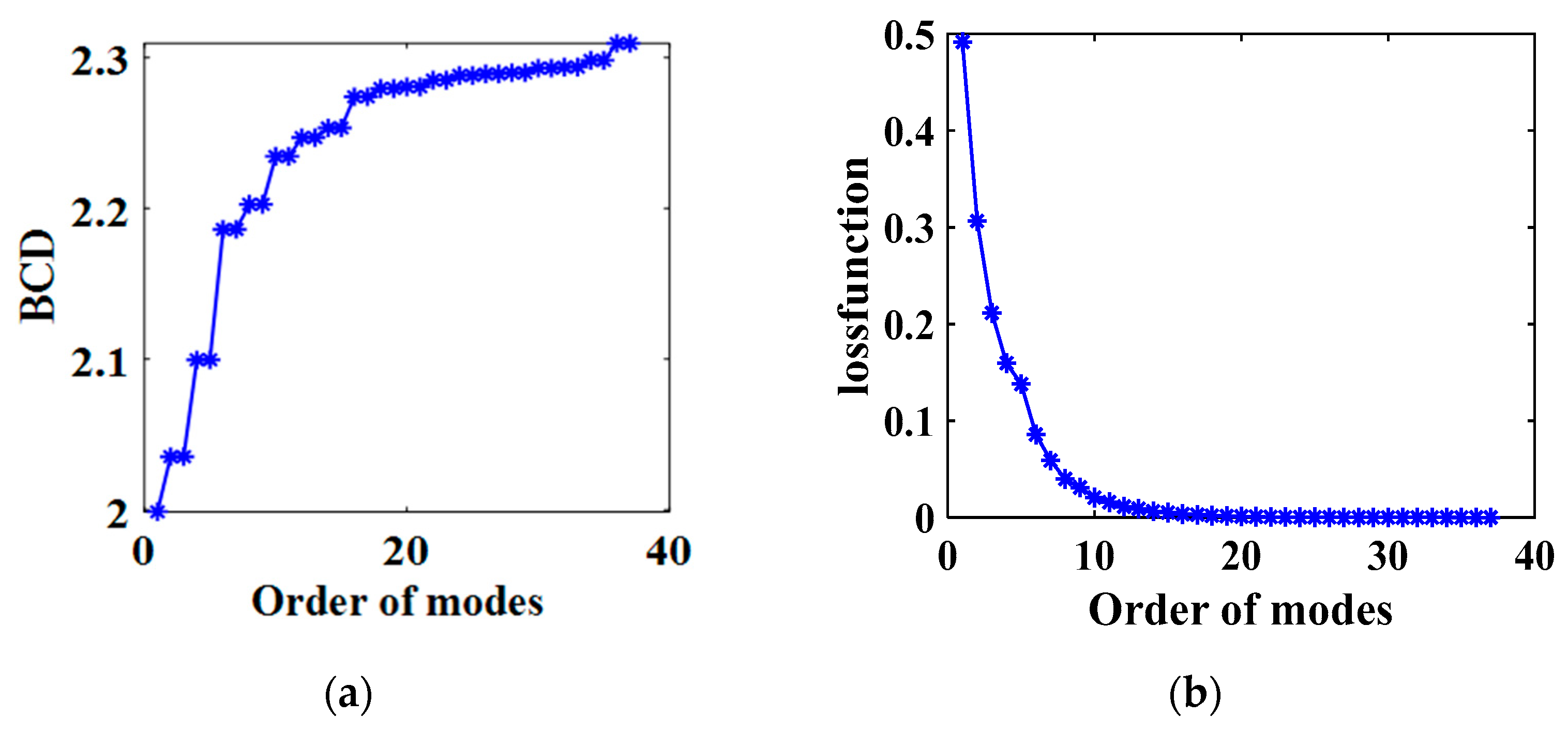
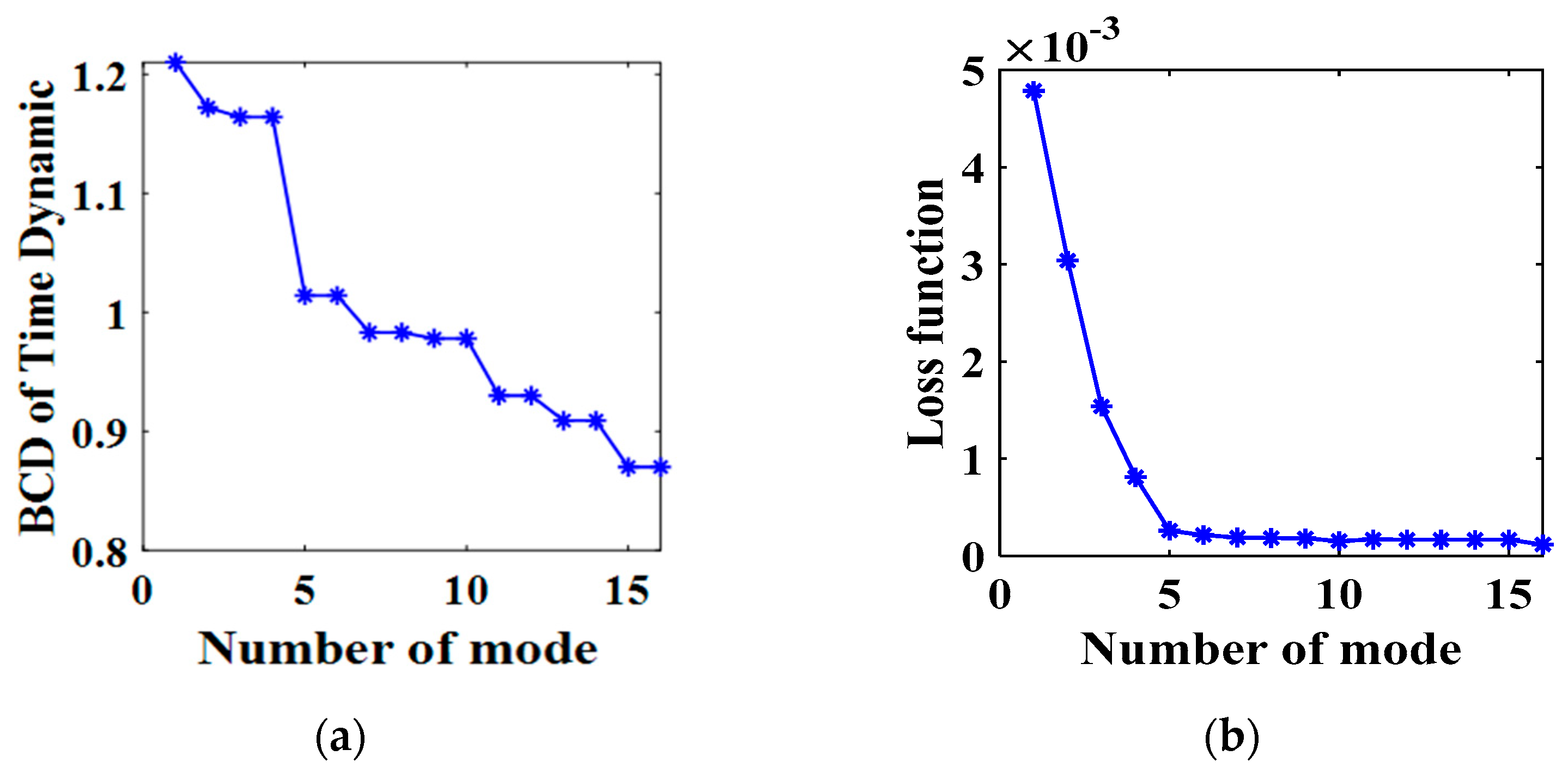
3.3.1. Modal Ranking Criterion Based on Box Counting Dimension

The flowchart of the modal reduction strategy based on fractal dimension (FDDMD) is presented in Figure 5. The calculation process involves two steps of reduction. The first procedure is applied to the snapshot matrix composed from timestep 1 to N − 1, where the singular value decomposition is carried out. The matrix is truncated by discarding items with eigenvalues smaller than ${10}^{-1}$. After truncation, the matrix is reduced to 31 dimensions, which represents the fundamental motion of the system and reflects the periodic motion variations of vortex shedding. The particularity of static modes represents the equilibrium state of the system. Since the first mode extracted from the mode decomposition is usually the static mode, the analysis is focused on subsequent modes.

The spatial structure distribution of the dynamic modes obtained by the DMD is shown in Figure 6, which exhibits strong fractal properties. Therefore, we separately calculate the box dimension for the different modes and take the average value as a representative of the fractal features of that mode.

In this context, a loss function is introduced as a reference to assess the quality of the reconstructed flow field. The loss function is described as follows:

$$lossfunction=\sqrt{\frac{{‖X-\Phi \mathrm{diag}(\alpha )V_{\mathit{and}}‖}_F^2}{‖X_F^2‖}}$$

(20)

In Figure 7, the horizontal axis is different modes and the vertical axis is the BCD corresponding to the modes. In addition to the dominant mode, most of the DMD modes are conjugate modes. The eigenvalues of the conjugate modes are the same as the real part of the modes themselves, and the imaginary part of the conjugate modes is the opposite of each other. Figure 7a reveals that the BCD of the higher frequency modes is stable around 2.3. In Figure 7b, by calculating the loss function for the sorted modes, it can be found that the BCD can sort the importance of the modes better. It is indicated that this sorting method is rational.

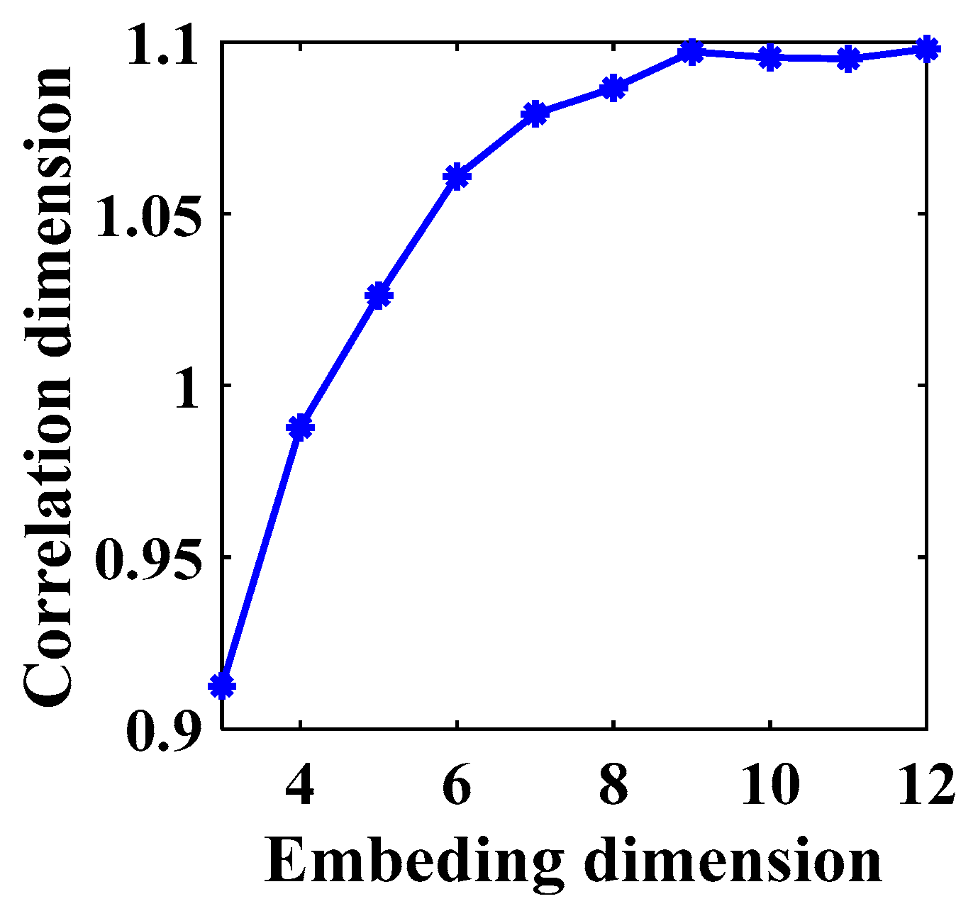
3.3.2. Modal Interception Criterion Based on Correlation Dimension

To improve subsequent system modeling, it is necessary to rank the importance of the decomposed modes. Choosing more modal orders leads to higher accuracy in the restored flow system. However, it also requires processing more data, which in turn reduces efficiency. The phase space of a dynamical system determines the geometric space of the system state. The phase space reconstruction theory based on Takens’s theorem [18] is a powerful tool for studying nonlinear dynamic systems. For a dynamic system with d degrees of freedom, an observation sequence embedded in a suitable manner ensures the trajectories of the system remain locally invariant. Hence, the determination of the appropriate embedding dimension m for the phase space has significance for estimating the degrees of freedom of the original dynamic system.

For the phase space reconstruction of multivariate time series, Cong [19] proposed a data fusion method. The specific process begins with the extraction of principal components from a multivariate time series. The time delay and embedding dimension for the r principal components are estimated using mutual information and a false nearest neighbor algorithm. Then, the corresponding phase points are fused based on Bayes estimation to obtain the reconstructed phase space of the original system.

Principal component analysis is performed on the row vectors of the matrix with the selection of 43,540 principal components. The time delay and embedding dimension m for each principal component are identified in Figure 8, with a minimum time delay of one and a maximum embedding dimension m of eight. Data fusion is performed subsequently for the phase points in the phase space to obtain the reconstructed phase space of the original system. The phase spaces mainly exhibit two distinct patterns in Figure 9.

Based on Bayes’s estimation, phase trajectory in the fused phase space is acquired in Figure 10. It is indicated that the fused phase space contains the main features of the original component time series in a comprehensive way.

Due to the large amount of data, the selection of the maximum embedding dimension as the global input of the original system will lead to certain errors. Therefore, the saturated correlation dimension is adopted to further confirm the option of embedding dimension [20]. The value of embedding dimensions from eight to eighteen and the time delay of two are chosen for the reconstruction of the phase space. The CD is revealed in Figure 11.

When the embedding dimension is 16, the correlation dimension reaches saturation. With a further increase in the embedding dimension, the CD shows a minor fluctuation around 1.3. Therefore, according to Takens’s theorem, the estimated degrees of freedom in the original system should be less than 7.5. Considering the BCD and loss function of the modes in Figure 7, the first seven orders of modes exhibit stronger fractal characteristics, and the loss function decreases gradually. Therefore, it is reasonable to intercept the first seven modes to restore the flow field. The reduction model for the flow system is represented in Figure 12 with a random moment. With the comparison with the original flow field, it can be observed that the main features are effectively extracted by this reduction method with dynamic modal decomposition by fractal dimension analysis.

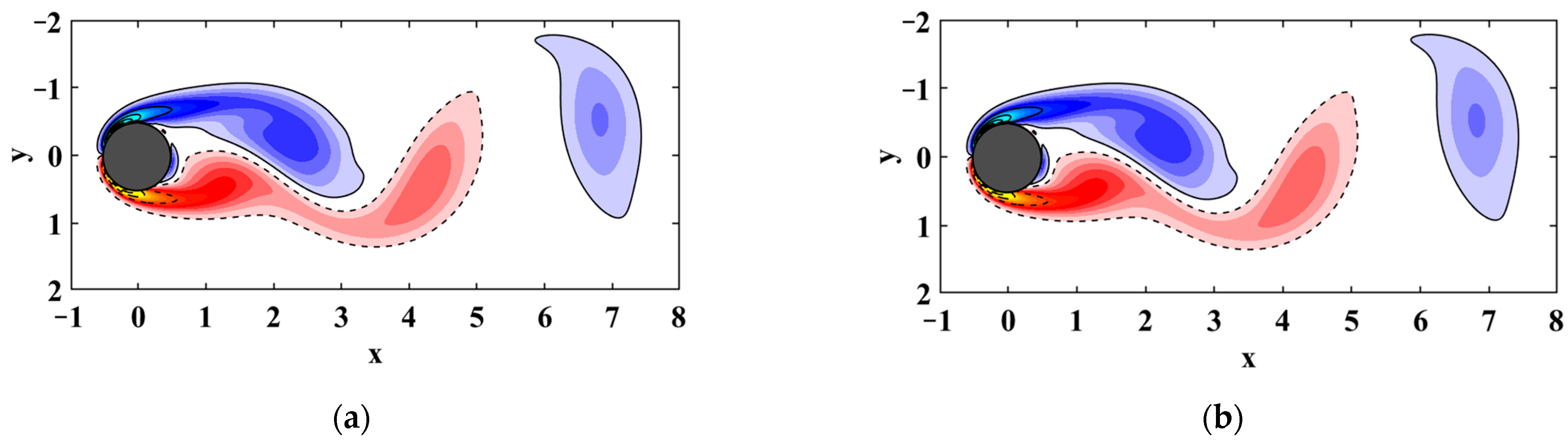
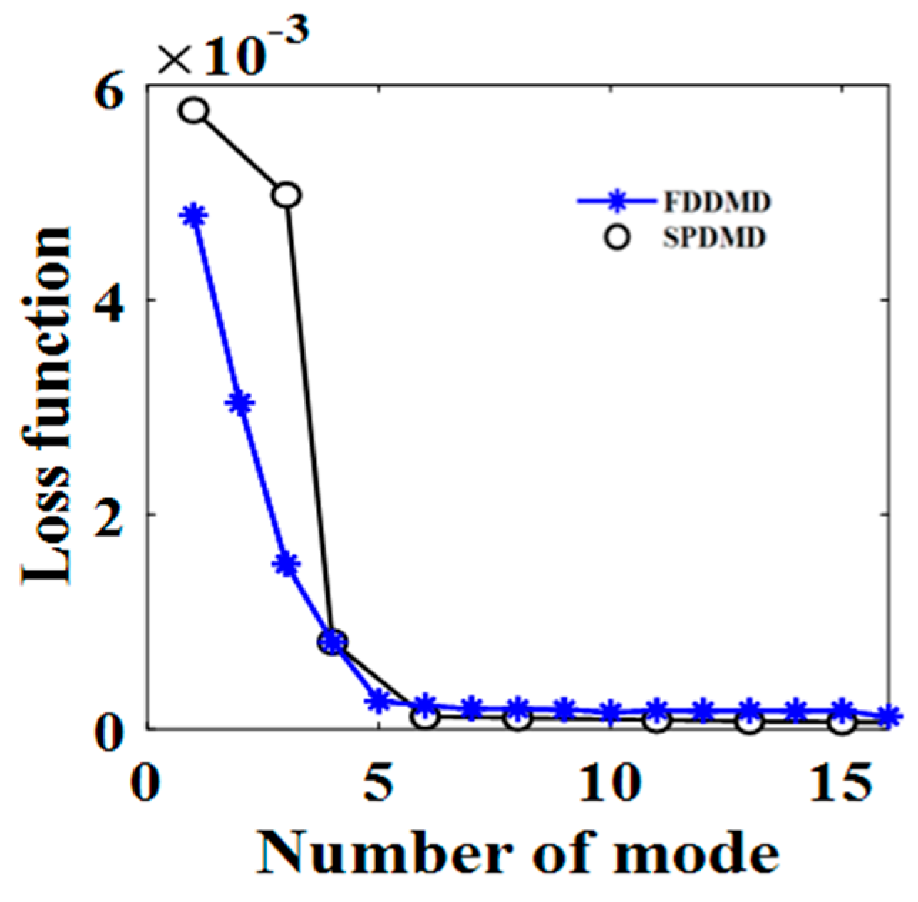
3.4. Comparison with Sparsity Promoting Dynamic Mode Decomposition (SPDMD)

SPDMD is the technique to screen for major patterns of DMD modes. The main difference between SPDMD and DMD is the definition of amplitude $\alpha$ in Equation (18). Instead of considering $\alpha$ to be the contribution of each mode to the initial flow field, SPDMD constructs an optimization problem. The sparse structure is determined in the optimization by adding a regular term $\alpha$, and the amplitude is continuously corrected for the solution. Finally, the modal order is selected by using the loss curves of different numbers of modes. Therefore, the selection of a subset of DMD modes for SPDMD is divided into two steps [10]. First, a sparsity structure is sought to realize a user-defined tradeoff between the number of extracted modes and the approximation error. Second, the sparsity structure of the vector of amplitudes is fixed and the optimal values of the non-zero amplitude are determined. Figure 13 indicates the loss curve of SPDMD.

Compared to the proposed FDDMD, the improvement of flow reduction is very limited by the amplitude optimization process of SPDMD. The modal intercept of SPDMD is determined based on a fixed residual threshold or the residual image inflection point.

Table 1. Mode selection by SPDMD and FDDMD.

	SPDMD	FDDMD
Number of Modes	7 or 9 or 11 or 13 or 15	8

indicates the mode selection by SPDMD and FDDMD. When selecting the modal order through the loss curve obtained by the SPDMD method, it is reasonable to select 7 or 15 modes. Therefore, it is difficult to uniquely determine the order, and it is also unconvincing to make a choice based on the loss curve. Through the embedding dimension analysis of the original system, FDDMD can uniquely determine the modal order with a certain degree of interpretability.

4. Application of Fractal Dimension on Aerodynamic Force Reduction

4.1. Data Collection

The highly accurate data is the basis for the reduction modeling of the aerodynamic force on the blade. In this paper, the reduction approach is mainly driven by the data achieved from the fluid-structure coupling computation [21]. The research target is a 1.5-stage axial compressor displayed in Figure 14 with part of the computation domain, including struts, inlet guide vanes, rotor, and stator.

The numerical solution of the 3D Navier–Stokes equations was solved by using the ANSYS 10.0 Package software. It employed a spatial discretization of the fluid equations in the upwind scheme and integrated a second-order backward differential for the diffusive term solution. For every rotor passage, it was divided into 40 timesteps with each timestep for 1.54875 × 10⁻⁵ s. Considering the fluid-structure interaction, the structural equations for mechanical blades were solved simultaneously with the flow equations by the finite element method within each timestep. The information between equations was exchanged on the fluid-structure interface. This procedure of the current timestep was repeated until the flow system was converged, before proceeding to the next timestep.

The 2017 sample points are selected in each blade on both the pressure side and the suction side. The snapshot data are captured for each timestep to obtain the distribution of aerodynamic force under the coordinates and construct a high-fidelity database. A total of 40 flow field snapshots in one revolution are selected with 3D coordinates as input, which is in accordance with previous research [22]. The variable quantity of Force is set as output to constitute the sample data $S=(X,Y,Z,Force)$. The extracted flow field snapshots are arranged according to time series

$$S_i=(X_{ij},Y_{ij},Z_{ij},Forc{e}_{ij})i=1,2,\dots ,40;j=1,2,\dots ,2017,$$

(21)

where i denotes the chord position of the blade and j denotes the spanwise position.

Figure 15 reveals the distribution of aerodynamic force on the blade surfaces at one timestep. It can be observed that at this current state, the value of aerodynamic force on the pressure side is apparently higher than that on the suction surface, which reflects a strong three-dimensional effect. It shows a nonlinear state exhibited by the aerodynamic force acting on the blade, resulting in a complex dynamic behavior of the system.

4.2. DMD Analysis of the Aerodynamic Force on the Blade

Figure 16 shows the distribution of the eigenvalues of the DMD modes. In Figure 16a, the eigenvalues are distributed within the unit circle, indicating neutral stability. In Figure 16b, the eigenvalues with the logarithm are distributed near the origin line. This means that the modes are neutral and stable [23]. A clear peak in the modal amplitude appears, corresponding to the dominant frequency (Figure 17a). There is a significant difference in the contribution levels of different modes to the initial flow field. It suggests that the main features may be dominated by a smaller number of modes.

4.3. Reduction Strategy for Aerodynamic Force Model

4.3.1. Modal Ranking Criterion Based on Box Counting Dimension

Similar to the process in Section 3, the matrix decomposition for aerodynamic force data also involves two reduction steps. The first step is to perform singular value decomposition on the snapshot matrix composed of timestep 1 to N − 1. The eigenvalues smaller than ${10}^{-2}$ are truncated, reducing the dimension to 16. The next step continues to reduce the dimension further for the second time. The original system can be considered as a combination of static and periodic modes. The analysis focuses on modes 2 to 16. Therefore, the fractal analysis is conducted on the evolution process of each mode. Figure 18 indicates the real and imaginary parts of the evolution features of some modes.

It is obvious that the amplitude of the evolution characteristic of the mode is gradually approaching zero. Reflected by Figure 18, it can be concluded that the slower the speed at which the amplitude of evolution approaches zero, the greater the role of the mode acts in the flow system. This can be quantitatively represented by the BCD based on a fixed radius centered at the origin. When the BCD of the fixed radius is small, it indicates that the data are more concentrated within the given radius.

The BCD of the point sets formed by the evolution characteristics of different orders of modes are calculated. It is arranged in a descending order, as shown in Figure 19a. The loss function with the reconstruction of the flow system is expressed in Figure 19b by the mode superposition. It is evident that this ranking method appears to be logical and effective.

4.3.2. Modal Interception Criterion Based on Correlation Dimension

In this section, the time delay and embedding dimension are estimated by mutual information method and false nearest neighbor algorithm for each time series sampling. After computation, the minimum time delay is identified as one, with the recognition of the maximum embedding dimension as six, as illustrated in Figure 20.

Under the condition of the time delay parameter chosen to be one, the correlation dimensions of the flow system are calculated successively with embedding dimensions ranging from three to twelve separately. As plotted in Figure 21, it is evident that the variation in the correlation dimension gradually stabilizes as the embedding dimension increases to nine. Therefore, on the basis of the saturated correlation dimension algorithm, an appropriate embedding dimension of nine is determined for reconstructing the original system.

When the embedding dimension is nine, the correlation dimension reaches saturation. With a further increase in the embedding dimension, the correlation dimension shows a minor fluctuation around 1.1. According to Takens’s theorem, it is estimated that the degrees of freedom of the original system are no more than four. Based on the loss function in Figure 19, the first four dynamic modes and the static mode are extracted to reconstruct the aerodynamic blade force. It can be observed from Figure 22 that the reconstructed system matches well with the original distribution of aerodynamic force. It is reasonable to believe the proposed approach for the reduction model is effective by the specified mode selection strategy of fractal dimension. With reconstruction modeling of complex aerodynamic force, it can be reduced by selecting the first four modes to represent the high-order system.

4.4. Comparison with SPDMD

In Figure 23, the loss function convergence of FDDMD is compared to SPDMD with the selected DMD modes. It is clear that there is a significant difference in the accuracy of the approximate model at the initial stage. This also highlights the importance of modal interception strategy on modeling accuracy. By observing the selected modes in Figure 24, it is found that the 2nd and 3rd modes selected by SPDMD are conjugate modes, and the 4th mode is the zero-frequency mode. However, FDDMD is able to proactively select the modes that contribute significantly to the system. Therefore, the proposed FDDMD has the advantage for the identification of the fractal characteristic of the mode evolution situation and can provide the reliable selection basis of the main modes for system reconstruction.

5. Discussion

The methodology proposed in this paper introduces two information fusion analyses, DMD and FD, for system assessment. It highlights the complementary advantage of bridging, which brings in system reconstruction applications. The trait of this research finds expression in its discussions on the analysis of the freedom degrees of the original system and the distinct fractal characterization of the main modes. The interpretability of the DMD selection is enhanced from a mathematical perspective.

There exist potential limitations to our current approach. Further attention can be given to the interaction influence between modes of the system, particularly regarding the interdependence effect on mode selection. In the analysis of fractal dimension, the BCD calculation is stricter for the box radius selection range. Therefore, further study on the rapid and accurate determination of the radius of the range is of worth.

In addition, there are several potential works in the future. Firstly, it could focus on further investigating the reduced order model regarding ordering and interception. Secondly, the fractal features of the principal modes identified in this study can be utilized as input features for training and analyzing artificial intelligence models to construct predictive models for the system.

6. Conclusions

In this paper, we propose a reduced-order analysis process for embedded systems based on the DMD method by exploring the fractal characteristics of hydrodynamic systems. Through the analysis of specific application cases, the feasibility of this technique is verified. The main conclusions are summarized as follows:

(1)

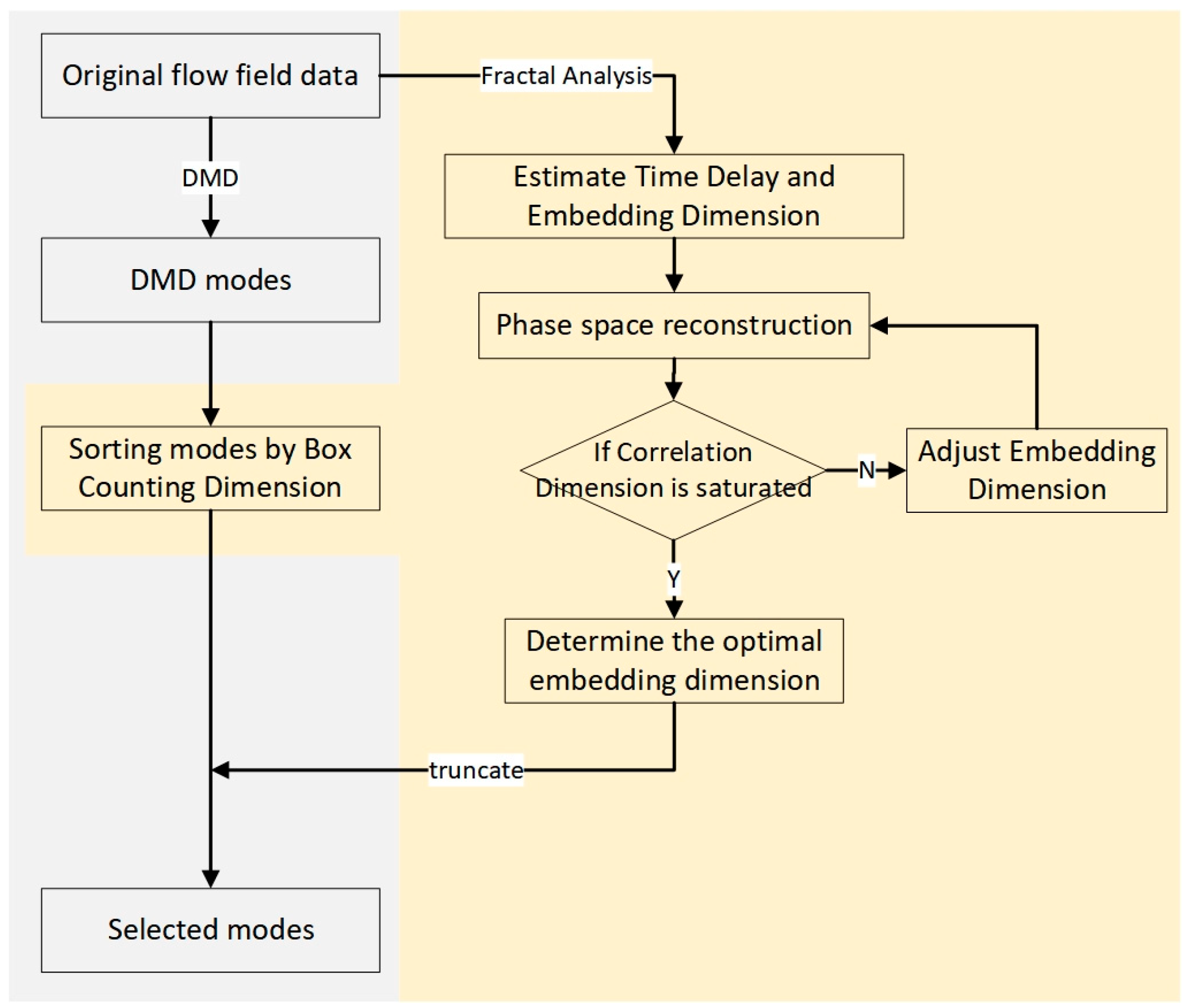
In DMD, previous methods of modal selection suffer from the defects of ignoring the detailed information of the source system as well as the arbitrariness of modal interception. To address this problem, we embed the fractal dimension theory into the DMD process from the perspective of fractal analysis, forming a reduced-order analysis process for embedded systems. This innovation makes the key model selection more interpretable and geometrically meaningful.

(2)

For the system of a cylinder wake velocity field, the first seven modes sorted by analysis of BCD are intercepted. It is found that the trajectory of the system motion can be recovered when the original system is projected into a seven-dimensional space, and the loss function of the intercepted modes can be reduced to about 5%. The main features can be well extracted by the DMD with fractal dimension embedding.

(3)

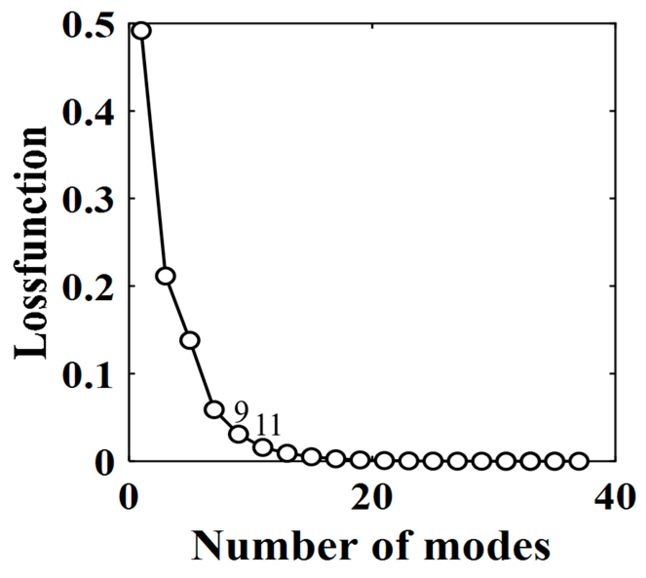
The reduction modeling of the aerodynamic force is performed with fractal dimension embedding. By the visualization of the fractal features of the system, the aerodynamic force can be well restored by a four-dimensional space projection. The error of the reduction model is less than 1%. It is reasonable to believe that the proposed approach for the reduction model is effective by the mode selection strategy of fractal dimension.

References

1. Chen, Y.; Tang, Y.; Lu, Q. Modern analytical methods in nonlinear dynamics. Intell. (Mech.) Mater. Struct. Sci. 1992, 1. [Google Scholar]
2. Dowell, E.H. Eigenmode analysis in unsteady aerodynamics: Reduced order models. AIAA J. 1996, 34, 1578–1583. [Google Scholar] [CrossRef]
3. Silva, W.A. Identification of linear and nonlinear aerodynamic impulse responses using digital filter techniques. AIAA 1997, 3712. [Google Scholar] [CrossRef]
4. Schmid, P.J.; Sesterhenn, J. Dynamic mode decomposition of numerical and experimental data. J. Fluid Mech. 2010, 656, 5–28. [Google Scholar] [CrossRef]
5. Gao, H.J.; Wang, T. Study on early-warning prediction of deep excavation settlement stability based on data dynamic mode decomposition. Geotech. Investig. Surv. 2023, 51, 35–41. [Google Scholar]
6. Chen, J.X.; Jiang, D.; Zhang, X.Y. Reconstruction of temporal and spatial distribution characteristics of sea surface temperature in the Yangtze River Estuary based on dynamic mode decomposition method. J. ZheJiang Univ. (Sci. Ed.) 2022, 49, 76–84. [Google Scholar]
7. Rowley, C.W.; Mezić, I.; Bagheri, S.; Schlatter, P.; Henningson, D.S. Spectral analysis of nonlinear flows. J. Fluid Mech. 2009, 641, 115–127. [Google Scholar] [CrossRef]
8. Schmid, P.J.; Violato, D.; Scarano, F. Decomposition of time-resolved tomographic PIV. Exp. Fluids 2012, 52, 1567–1579. [Google Scholar] [CrossRef]
9. Sayadi, T.; Schmid, P.J.; Nichols, J.W.; Moin, P. Reduced-order representation of near-wall structures in the late transitional boundary layer. J. Fluid Mech. 2014, 748, 278–301. [Google Scholar] [CrossRef]
10. Jovanović, M.R.; Schmid, P.J.; Nichols, J.W. Sparsity-promoting dynamic mode decomposition. Phys. Fluids 2014, 26, 024103. [Google Scholar] [CrossRef]
11. Tu, J.H.; Rowley, C.W.; Luchtenburg, D.M.; Brunton, L.S.; Kutz, N.J. On dynamic mode decomposition: Theory and applications. J. Comput. Dyn. 2014, 1, 391–421. [Google Scholar] [CrossRef]
12. Tissot, G.; Cordier, L.; Benard, N.; Bernd, R.B. Model reduction using dynamic mode decomposition. Compt. Rendus Méc. 2014, 342, 410–416. [Google Scholar] [CrossRef]
13. Sayadi, T.; Schmid, P.J.; Richecoeurj, F.; Durox, D. Parametrized data-driven decomposition for bifurcation analysis, with application to thermo-acoustically unstable systems. Phys. Fluids 2015, 27, 037102. [Google Scholar] [CrossRef]
14. Kou, J.Q. Reduced-Order Modeling Methods for Unsteady Aerodynamics and Fluid Flows. J. Northwest. Polytech. Univ. 2018. [Google Scholar] [CrossRef]
15. Krake, T.; Reinhardt, S.; Hlawatsch, M.; Eberhardt, B.; Weiskopf, D. Visualization and selection of Dynamic Mode Decomposition components for unsteady flow. Vis. Inform. 2021, 5, 15–27. [Google Scholar] [CrossRef]
16. Zhu, H.; Ji, C.C. Fractal Theory and Its Applications; Science Press: Beijing, China, 2011. [Google Scholar]
17. Kutz, J.N.; Steven, L.B.; Bingni, W.B.; Joshua, L.P. Dynamic Mode Decomposition; Society for Industrial and Applied Mathematics: Philadelphia, PA, USA, 2016. [Google Scholar]
18. Takens, F. Dynamical Systems and Turbulence, Warwick 1980; Springer: Berlin/Heidelberg, Germany, 2006. [Google Scholar]
19. Cong, R.; Liu, S.L.; Ma, R. An approach to phase space reconstruction from multivariate data based on data fusion. Chin. J. Phys. 2008, 57, 7487–7493. [Google Scholar] [CrossRef]
20. Lv, J.H.; Lu, J.A.; Chen, Z.H. Chaotic Time Series Analysis and Its Applications; Wuhan University Press: Wuhan, China, 2002. [Google Scholar]
21. Zhang, M.M.; Hou, A.P. Investigation on the Flow Field Entropy Structure of Non-Synchronous Blade Vibration in an Axial Turbo compressor. Entropy 2020, 22, 1372. [Google Scholar] [CrossRef] [PubMed]
22. Zhang, M.M.; Hao, S.R.; Hou, A.P. Study on the Intelligent Modeling of the Blade Aerodynamic Force in Compressors Based on Machine Learning. Mathematics 2021, 9, 476. [Google Scholar] [CrossRef]
23. Hemati, M.S.; Williams, M.O.; Rowley, C.W. Dynamic mode decomposition for large and streaming datasets. Phys. Fluids 2014, 26, 111701. [Google Scholar] [CrossRef]
Figure 1. Flowchart of the system reduction with fractal dimension embedding.
Fractalfract 08 00331 g001
Figure 2. Instantaneous circular cylinder vortex snapshot in a flow field.
Fractalfract 08 00331 g002
Figure 3. The real and imaginary parts of the DMD eigenvalues: (a) non-logarithmic eigenvalue distribution; (b) logarithmic eigenvalue distribution.
Fractalfract 08 00331 g003
Figure 4. Amplitude distribution of the DMD: (a) the corresponding frequency; (b) growth rate.
Fractalfract 08 00331 g004
Figure 5. The flowchart of the modal reduction strategy.
Fractalfract 08 00331 g005
Figure 6. Dynamic modal decomposition on the fluid vorticity field: (a) the 2nd mode; (b) the 6th mode; (c) the 14th mode; (d) the 28th mode.
Fractalfract 08 00331 g006
Figure 7. Sorted DMD modes: (a) BCD of each mode; (b) loss function.
Fractalfract 08 00331 g007
Figure 8. The parameters of all principal components: (a) time delay; (b) embedding dimension.
Fractalfract 08 00331 g008
Figure 9. Reconstruction plots with principal components: (a) X1 time series; (b) X1527 time series.
Fractalfract 08 00331 g009
Figure 10. Reconstructed map of the original system.
Fractalfract 08 00331 g010
Figure 11. Embedding dimension–correlation dimension diagram.
Fractalfract 08 00331 g011
Figure 12. Flow reconstruction with DMD: (a) the original field; (b) the reconstructed field.
Fractalfract 08 00331 g012
Figure 13. Loss function for the sorted SPDMD modes.
Fractalfract 08 00331 g013
Figure 14. Computation domain of the research target [22].
Fractalfract 08 00331 g014
Figure 15. Distribution of aerodynamic force on the blade: (a) pressure side; (b) suction side.
Fractalfract 08 00331 g015
Figure 16. The DMD eigenvalues on the unit circle: (a) non-logarithmic eigenvalue; (b) logarithmic eigenvalue.
Fractalfract 08 00331 g016
Figure 17. Amplitude distribution of the DMD modes: (a) frequency; (b) growth rate.
Fractalfract 08 00331 g017
Figure 18. Fractal features of modes in the evolution process: (a) 1st mode; (b) 6th mode; (c) 10th mode; (d) 16th mode.
Fractalfract 08 00331 g018
Figure 19. Sorted DMD modes: (a) BCD of each mode; (b) loss function.
Fractalfract 08 00331 g019
Figure 20. Parameters with principal components: (a) embedding dimension; (b) time delay.
Fractalfract 08 00331 g020
Figure 21. Embedding dimension–correlation dimension diagram.
Fractalfract 08 00331 g021
Figure 22. Distribution of force on pressure surface: (a) reduction model; (b) CFD simulation.
Fractalfract 08 00331 g022
Figure 23. Variations of the loss function with FDDMD and SPDMD.
Fractalfract 08 00331 g023
Figure 24. Mode order for different mode selection methods. (a) FDDMD; (b) SPDMD.
Fractalfract 08 00331 g024