Novel Admissibility Criteria and Multiple Simulations for Descriptor Fractional Order Systems with Minimal LMI Variables

Abstract

In this paper, we first present multiple numerical simulations of the anti-symmetric matrix in the stability criteria for fractional order systems (FOSs). Subsequently, this paper is devoted to the study of the admissibility criteria for descriptor fractional order systems (DFOSs) whose order belongs to (0, 2). The admissibility criteria are provided for DFOSs without eigenvalues on the boundary axes. In addition, a unified admissibility criterion for DFOSs involving the minimal linear matrix inequality (LMI) variable is provided. The results of this paper are all based on LMIs. Finally, numerical examples were provided to validate the accuracy and effectiveness of the conclusions.

1. Introduction

Fractional calculus (FC) has a history of three centuries, and many researchers have studied and discussed it as a purely theoretical field. In recent years, it has become increasingly recognized that many dynamical systems can be more accurately described using FC and integrals rather than conventional integer-order models [1]. FOSs are also widely used in fuzzy systems [2,3], switching systems [4,5], robust control [6,7], and other fields [8,9]. In addition, recent studies have made advancements in analyzing the stability and performance of FOSs and applying them to more complex real-world systems [10]. For example, [4] applied switched FOSs to an $R{L}_{\beta }{C}_{\alpha }$ circuit and accurately portrayed the relationship between voltage and current in the circuit to obtain the switching rate. Xu et al. [11] developed a fractional derivative model to describe the complex viscoelastic creep behaviors of Hami Melon.

Stability is a fundamental property of control systems [12,13,14]. For FOSs, Matignon [15] proposed the first stability criterion, indicating that the stability problem of FOSs can be attributed to the eigenvalue problem of the pseudo-state matrix. Although this criterion theoretically analyzed stability, the design of the controller remains challenging. Oustaloup et al. [16] pioneered the famous CRONE control technique, making controller design and control simulation possible but still not based on LMIs. Since then, FOSs have entered the field of automatic control. Building upon this foundation, Farges et al. [17] concentrated on formulating LMI conditions to ensure the stability of commensurate FOSs through the application of two complex variables. In [18], an approach leveraging an LMI-based stability criterion, which utilizes a reduced number of real variables, was proposed for solving convex optimization problems, ultimately facilitating the design of the controller. In the latest study, a practical stability condition for FOSs is presented, employing the LMI method. Convex optimization problems involving LMIs can represent numerous issues in control theory. This approach has enhanced the efficacy of solving control theory-related problems since the early 1990s. Based on this approach, refs. [19,20,21,22,23,24] focused on the stability of FOSs with order $\alpha \in [1,2)$ and $\alpha \in (0,1)$, respectively. However, the decision matrices were either too complex in form or too numerous in quantity in the stability criteria for the FOSs mentioned above, making these criteria too complex and not conducive to controller design [25]. Zhang et al. [26] recently derived a set of LMI-based criteria for the stability and stabilization of FOSs with fractional order $\alpha$ belonging to the interval $(0,2)$, which involves minimal real LMI variables.

It is well known that for descriptor systems, admissibility is a very important property. Therefore, in addition to stability, we need to consider regularity and non-impulsivity [27,28]. There are a large number of achievements in the area of admissibility [29,30,31,32,33,34,35]. For DFOSs with orders $\alpha \in [1,2)$, admissibility criteria based on a set of strict LMIs representations were given in [36,37], respectively. For orders belonging to $(0,1)$, Marir et al. [35] proposed an observer-based controller to ensure the admissibility of DFOSs. However, the results in [35] involved both complex numbers and complex matrices, making it challenging to determine feasible solutions. In [38], the investigation delved into admissibility and robust stabilization criteria for DFOSs within the order range of $(0,1)$. This was accomplished through the application of a method employing strict LMIs with real matrices, facilitating straightforward solutions. N’Doye et al. [39] focused on DFOSs with order $\alpha \in (0,2)$. However, only sufficient conditions were given. For DFOSs with a given fractional order belonging to $(0,2)$, Wang et al. [40] provided admissibility and quadratic admissibility criteria. However, their approach involved multiple real decision variables.

Although there are many results on the stability criteria for FOSs, the simulation of the antisymmetric matrix in the criteria is a challenge. In this regard, we provide a variety of simulations. There are many results on the admissibility criteria for DFOSs, but for DFOSs without eigenvalues on the boundary axes, no report on the admissibility criterion using the LMI expression was found. Meanwhile, there are few reports on the admissibility criteria using the minimal LMIs variable. Inspired by the above discussion, this paper proposes novel admissibility criteria by converting the assumption that there are no eigenvalues on the boundary axes to LMIs. Subsequently, this paper derives a new criterion on the DFOSs admissibility condition of fractional order $\alpha \in (0,2)$ in a more concise form than [41]. The contributions of this paper are as follows:

(1)

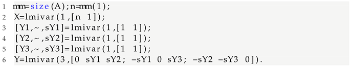
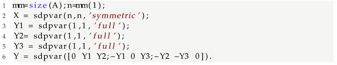
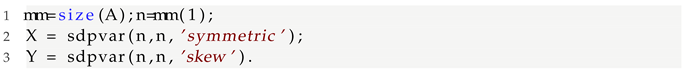
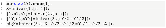
The simulation of the anti-symmetric matrix within the stability criteria based on LMIs for FOSs has consistently presented challenges. This paper addresses these challenges by utilizing MATLAB, offering a range of simulation methods employing both the LMI toolbox and the YALMIP toolbox.

(2)

There are a large number of results for the admissibility criteria for DFOSs with eigenvalues not on the boundary axes, but none of them deal with them directly using LMIs. This paper advances this area by converting this hypothetical condition into LMI-based admissibility criteria, thus making it easy to use MATLAB to determine feasible solutions.

(3)

Previously proposed admissibility criteria for DFOSs include several decision variables and even involve complex variables, making it difficult to determine feasible solutions using MATLAB. The admissibility criteria proposed in this paper involve the minimal LMIs variable, which makes it easy to determine feasible solutions.

(4)

Diverging from the methodologies of existing algorithms, which segregate the interval $(0,2)$ into two distinct ranges: $(0,1)$ and $[1,2)$, this research constructs an LMI structure, which is applicable to DFOSs with $0<\alpha <2$.

(5)

The admissibility criteria derived in this paper, through the application of methodologies including contract transformation, are contingent solely upon factors such as fractional order, the pseudo state matrix, and the direction of control.

The paper is organized as follows. Section 2 introduces several preliminary results. Section 3 presents our main results for FOSs and DFOSs. In Section 4, we validate the theoretical results through numerical examples. Finally, Section 5 concludes the paper.

Notations: Let ${\mathbb{C}}^{n\times n}({\mathbb{R}}^{n\times n})$ denote the set of complex (real) matrices with dimensions $n\times n$. For $0<\alpha <2$, $a=sin(\frac{\pi \alpha }{2})$, $b=cos(\frac{\pi \alpha }{2})$, $\Theta =\left[\begin{array}{cc}a& b\\ -b& a\end{array}\right]$. I denotes an identity matrix with appropriate dimensions. $X<0(>0)$ indicates that matrix X is negatively definite (positively definite). $X^T(X^{\ast })$ represents the transpose (transpose conjugate) of the matrix X. $\mathrm{sym}(X)=(X+X^T)$. $A\otimes B$ represents the Kronecker product of two matrices A and B. $\lceil \alpha \rceil$$(\lfloor \alpha \rfloor )$ denotes the largest (smallest) integer not greater than (not less than) $\alpha$.

2. Problem Statements and Preliminaries

Consider the unforced descriptor fractional order system

$$E{D}^{\alpha }x(t)=Ax(t),$$

(1)

where $A\in {\mathbb{R}}^{n\times n}$ is the constant matrix and $x(t)\in {\mathbb{R}}^n$ is the physical state vector. $E\in {\mathbb{R}}^{n\times n}$ is the singular matrix and $0<\mathrm{rank}(E)=m<n$. $D^{\alpha }f(·)$ is the Caputo fractional derivative with order $\alpha \in (0,2)$ of function $f(·)$.

Prior to deriving the admissibility criterion for DFOSs, we first introduce the following definition and lemmas.

Definition 1

([38]). System (1) is said to be regular if $\det \left(sE-A\right)\not\equiv 0$. System (1) is said to be impulse-free if $\mathrm{deg}\left(\det \left(sE-A\right)\right)=\mathrm{rank}\left(E\right)$. System (1) is said to be stable if $\left|\arg \left(\mathrm{spec}\left(E,A\right)\right)\right|>\alpha \frac{\pi }{2}$, where $\mathrm{spec}\left(E,A\right)$ is the spectrum (set of all roots) of $\det \left(sE-A\right)=0$. System (1) is said to be admissible if it is regular, impulse-free, and stable.

Lemma 1

([38]). If System (1) is regular, then there exist invertible matrices R and L such that

$$REL=\left[\begin{array}{cc}{I}_m& 0\\ 0& N\end{array}\right],RAL=\left[\begin{array}{cc}J& 0\\ 0& I_{n-m}\end{array}\right],$$

(2)

where N is a nilpotent matrix and

(1) 

System (1) with order $\alpha \in (0,2)$ is impulse-free if $N=0$;

(2) 

System (1) with order $\alpha \in (0,2)$ is stable if $\left|\arg \left(\mathrm{spec}\left(J\right)\right)\right|>\alpha \frac{\pi }{2}$;

(3) 

System (1) with order $\alpha \in (0,2)$ is admissible if it is impulse-free and stable.

Lemma 2.

For given $Z\in {\mathbb{C}}^{n\times n}$,

$$Z\ge 0,$$

(3)

if and only if

$$\left[\begin{array}{cc}\Re \left(Z\right)& -\Im \left(Z\right)\\ \Im \left(Z\right)& \Re \left(Z\right)\end{array}\right]\ge 0,$$

(4)

or

$$\left[\begin{array}{cc}\Re \left(Z\right)& \Im \left(Z\right)\\ -\Im \left(Z\right)& \Re \left(Z\right)\end{array}\right]\ge 0,$$

(5)

where $\Re \left(Z\right)(\Im \left(Z\right))$ is the real part (imaginary part) of Z.

Proof. 

Assume that Equation (3) holds, i.e., for $\forall z\in {\mathbb{C}}^n,z\ne 0$,

$$z^{\ast }\left(\Re \left(Z\right)+\mathrm{j}\Im \left(Z\right)\right)z\ge 0.$$

Therefore, by the property of conjugation, we obtain the following:

$$z^{\ast }\left(\Re \left(Z\right)-\mathrm{j}\Im \left(Z\right)\right)z\ge 0.$$

Namely,

$$\Re \left(Z\right)-\mathrm{j}\Im \left(Z\right)\ge 0.$$

(6)

Similarly, if Equation (6) holds, then Equation (3) holds. Therefore, it can be concluded that

$$\left[\begin{array}{cc}\Re \left(Z\right)+\mathrm{j}\Im \left(Z\right)& 0\\ 0& \Re \left(Z\right)-\mathrm{j}\Im \left(Z\right)\end{array}\right]\ge 0.$$

(7)

Pre- and postmultiplying (7) by

$$\frac{1}{\sqrt{2}}\left[\begin{array}{cc}I& I\\ \mathrm{j}I& -\mathrm{j}I\end{array}\right]$$

and its conjugate transpose, it can be inferred that Equation (4) holds. Subsequently, according to Theorem 1 in [15], Equation (5) holds. Conversely, Equation (3) can also be derived from Equations (4) or (5).    □

Lemma 3.

Matrix $A\in {\mathbb{R}}^{n\times n}$ is D-stable, as defined in [18], if and only if there exist $M,N\in {\mathbb{R}}^{\lceil \alpha \rceil n\times \lceil \alpha \rceil n}$, such that

$$I_{\lceil \alpha \rceil }\otimes A=MN,$$

(8)

where M is a generalized negative definite matrix satisfying the form

$$M={\Theta }_{\alpha }\otimes A\left(P_{\alpha }{E}^T+SQ\right),$$

and N satisfies the form

$$N={\Theta }_{\alpha }^{-1}\otimes {\left(P_{\alpha }{E}^T+SQ\right)}^{-1},$$

where ${\Theta }_{\alpha }=\Theta \left(\lceil \alpha \rceil \right),\Theta \left(1\right)=\det \left(\Theta \right),\Theta \left(2\right)=\Theta$, $Q\in {\mathbb{R}}^{(n-m)\times n}$, $S\in {\mathbb{R}}^{n\times (n-m)}$ is any matrix with a full column rank satisfying $ES=0$, $P_{\alpha }=a^{-\lfloor \alpha -1\rfloor }X+b\lfloor \alpha -1\rfloor Y\in {\mathbb{R}}^{n\times n}$, and

$$\left[\begin{array}{cc}X& Y\\ -Y& X\end{array}\right]>0.$$

Proof. 

(Necessity) In the case of $0<\alpha <1$, by Theorem 2.2 in [38], there exist $X_1,Y_1\in {\mathbb{R}}^{n\times n}\mathrm{and}Q\in {\mathbb{R}}^{(n-m)\times n}$ satisfying

$$\left[\begin{array}{cc}{X}_1& -Y_1\\ Y_1& X_1\end{array}\right]>0,$$

(9)

$$\mathrm{sym}\left(A\left(\left(a{X}_1-b{Y}_1\right)E^T+SQ\right)\right)<0.$$

(10)

Noting that $\left(a{X}_1-b{Y}_1\right)E^T+SQ$ is non-singular, let

$$P=a{X}_1-b{Y}_1,M=A(P{E}^T+SQ)\mathrm{and}N={\left(P{E}^T+SQ\right)}^{-1}.$$

Therefore, condition (8) holds.

In the case of $1\le \alpha <2$, by Theorem 2 in [36], there exist $X\in {\mathbb{R}}^{n\times n}\mathrm{and}Q\in {\mathbb{R}}^{(n-m)\times n}$ satisfying

$$X>0,$$

(11)

$$\mathrm{sym}\left(\Theta \otimes \left(A\left(X{E}^T+SQ\right)\right)\right)<0.$$

(12)

Let

$$P=X,M=\Theta \otimes A\left(P{E}^T+SQ\right)\mathrm{and}N={\Theta }^{-1}\otimes {\left(P{E}^T+SQ\right)}^{-1}$$

get condition (8) to hold.

(Sufficiency) The sufficiency of the theorem is proved according to the reverse process of the proof of necessity. In this way, the proof is complete.    □

Remark 1.

When the fractional order $\alpha =1$, Lemma 3 reduces to Theorem 3.1 in [12].

3. Main Results

Firstly, this section presents various numerical simulation methods for evaluating the stability criteria of fractional order systems (FOSs) with orders in the interval $(0,1)$. Then, new LMI-based admissibility criteria of order $(0,1)$ and $[1,2)$ are provided, and subsequently, admissibility criteria for DFOSs of order $(0,2)$ involving the minimal LMIs variable are given.

3.1. Multiple Simulations of Anti Symmetric Matrices in Stability Criteria of FOSs

If $E(=I)$ is a nonsingular matrix, System (1) reduces to a FOSs as follows:

$$D^{\alpha }x(t)=Ax(t).$$

(13)

For the seductiveness of System (13), Theorem 2.1 in [18] provides an effective LMI result. The feasible solution is solved using the MATLAB LMI toolbox. Relevant results are now provided to extend the LMI approach to simulation.

Theorem 1.

FOSs (13) with $\alpha \in (0,1)$ are asymptotically stable if there exist $X,Y\in {\mathbb{R}}^{n\times n}$, such that

$$\left[\begin{array}{cc}X& \frac{Y}{2}-\frac{Y^T}{2}\\ -\frac{Y}{2}+\frac{Y^T}{2}& X\end{array}\right]>0,$$

(14)

$$\mathrm{sym}\left(A\left(aX-b\left(\frac{Y}{2}-\frac{Y^T}{2}\right)\right)\right)<0.$$

(15)

Proof. 

Notice that, for any matrix $\widehat{Y}=\frac{Y}{2}-\frac{Y^T}{2}$, there is $\widehat{Y}=-{\widehat{Y}}^T$. Thus, in conjunction with Theorem 2.1 in [18], Theorem 1 holds.    □

Remark 2.

In contrast to Theorem 2.1 in [18], the result of Corollary 8 is more general since it does not require matrix Y to be a skew symmetry matrix.

Previous numerical simulation methods on LMI-based stability criteria are based on the MATLAB LMIs toolbox [18]. Now, based on the following example, we extend the numerical simulation method.

Example 1.

Consider the fractional-order system (13) with $\alpha =0.5$ and

$$A=\left[\begin{array}{cc}-5& -2\\ -1& -3.\end{array}\right]$$

By calculating the eigenvalues of A, it can be seen that the system is stable. Based on the above analysis, using the MATLAB commands in Appendix A, the corresponding feasible solutions are listed in

Table 1. Numerical simulation method and results.

LMIs in Stability Criterion	Matlab Toolbox	Matlab Commands	Feasible Solutions
LMIs of Theorem 2.1 in [18]	LMI Toolbox	Appendix A.1	$\begin{array}{cc}\hfill X& =\left[\begin{array}{ccc}23.9895& -8.7907& -8.5082\\ -8.7907& 37.4659& -2.4703\\ -8.5082& -2.4703& 22.0122\end{array}\right],\hfill \\ \hfill Y& =\left[\begin{array}{ccc}0& 8.3929& 4.3854\\ -8.3929& 0& -0.6818\\ -4.3854& 0.6818& 0\end{array}\right]\hfill \end{array}$
		Appendix A.2
	Yalmip	Appendix A.3
		Appendix A.4
LMIs (14) and (15) of Theorem 1	LMI Toolbox	Appendix A.5	$\begin{array}{cc}\hfill X& =\left[\begin{array}{ccc}0.8750& -0.3981& -0.2696\\ -0.3981& 1.1161& -0.0936\\ -0.2696& -0.0936& 0.6161\end{array}\right],\hfill \\ \hfill Y& =\left[\begin{array}{ccc}0& 94.2022& -135.6207\\ 0& 0& 11.7753\\ 0& 0& 0\end{array}\right]\hfill \end{array}$
	Yalmip	Appendix A.6	$\begin{array}{cc}\hfill X& =\left[\begin{array}{ccc}23.6587& -8.6255& -8.3580\\ -8.6255& 35.1317& -2.3350\\ -8.3580& -2.3350& 20.6241\end{array}\right],\hfill \\ \hfill Y& =\left[\begin{array}{ccc}34.2562& 41.3981& 37.5205\\ 27.1042& 34.2662& 33.5344\\ 30.9618& 34.8279& 34.2462\end{array}\right]\hfill \end{array}$

. The state diagram of the system in Example 1 is shown in Figure 1. It is evident that the system is stable.

Remark 3.

Referring to

Table 2. Comparison of our approach compared to existing approaches.

Ref.	Var.kind	Easy Solve	Variables	Less Conservative
[15]	NA	×	NA	×
[17]	$\mathbb{C}$	×	4	×
[20]	$\mathbb{R}$	×	4	×
[23]	$\mathbb{R}$	✓	1	×
[22]	$\mathbb{R}$	×	2	✓
[18]	$\mathbb{R}$	×	2	✓
ours	$\mathbb{R}$	✓	2	✓

, our approach involves the least number of actual decision variables, has low algorithmic complexity, reduces stabilisation conservatism, and does not involve an antisymmetric matrix, making it easy to solve for the decision variables. Overall, from the comparison in Table 2, our results outperform the existing results.

3.2. Admissibility Criteria Based on LMIs for DFOSs with Eigenvalues Not on Boundary Axes

For DFOSs without eigenvalues of the boundary axes, we propose novel LMIs based on admissibility criteria. Firstly, the admissibility criteria for SOFS of order $\alpha \in [1,2)$ are as follows.

Theorem 2.

System (1) with $\alpha \in [1,2)$ is admissible if there exist $X\in {\mathbb{C}}^{n\times n},Y\in {\mathbb{R}}^{n\times n}$, such that

$$E^{T}X=X^{\ast }E,$$

(16)

$$\mathrm{sym}\left(\Theta \otimes A^{T}X\right)<0,$$

(17)

$$\mathrm{sym}\left(\Theta \otimes E^{T}Y\right)\le 0,$$

(18)

$$A^{T}Y=Y^{T}A>0.$$

(19)

Proof. 

(Sufficiency) Assume the existence of a complex matrix X, such that conditions (16)–(19) hold, respectively. According to condition (19), matrix A is nonsingular. Let $\lambda$ be the generalized eigenvalue of A, i.e.,

$$\lambda Ex=Ax,x\in {\mathbb{C}}^n.$$

Therefore,

$$\begin{array}{cc}\hfill & \left(I\otimes x^{\ast }\right)\left(\Theta \otimes A^{T}X+{\Theta }^T\otimes X^{\ast }A\right)\left(I\otimes x\right)\hfill \\ \hfill =& \Theta \otimes \left(x^{\ast }{A}^{T}Xx\right)+{\Theta }^T\otimes \left(x^{\ast }{X}^{\ast }Ax\right)\hfill \\ \hfill =& x^{\ast }{E}^{T}Xx\left(\overline{\lambda }\Theta +\lambda {\Theta }^T\right)<0.\hfill \end{array}$$

(20)

Let

$$\frac{\Im \left(\lambda \right)}{\Re \left(\lambda \right)}=\frac{a}{b},$$

then the left side of Equation (20) is equivalent to

$$ab{x}^{\ast }{E}^{T}Xx\left[\begin{array}{cc}1& j\\ -j& 1\end{array}\right],$$

which has zero eigenvalue, making Equation (20) not hold. Similarly, Equation (20) does not hold when

$$\frac{\Im \left(\lambda \right)}{\Re \left(\lambda \right)}=-\frac{a}{b}.$$

Therefore, there is no characteristic root of triple $\left(E,A,\alpha \right)$ that falls on the line $y=\pm \tan \left(\alpha \frac{\pi }{2}\right)x,x<0$. By Theorem 10 in [31], System (1) is admissible if conditions (18) and (19) hold.

(Necessity) Suppose that System (1) is admissible. By Lemma 1, there exist $R,L$, such that

$$REL=\left[\begin{array}{cc}I& 0\\ 0& 0\end{array}\right],RAL=\left[\begin{array}{cc}J& 0\\ 0& I\end{array}\right].$$

(21)

By Lemma 1 in [26], there exists $X_1\in {\mathbb{R}}^{m\times m}$, satisfying Equations (11) and (12). Let

$$X=R^T\left[\begin{array}{cc}{X}_1& 0\\ 0& -I\end{array}\right]L^{-1},$$

by Theorem 10 in [31]. Combining Equations (11), (12), and (21) indicates that Equations (16)–(19) hold.    □

Remark 4.

Theorem 2 presents a novel admissibility criterion for DFOSs with the order in the interval $[1,2)$, thereby enriching the study of DFOS admissibility. However, Theorem 2 includes a complex variable, which poses challenges for numerical simulation.

On the basis of Theorem 2, some corollaries are given.

Corollary 1.

System (1) with $\alpha \in [1,2)$ is admissible if there exist $X\in {\mathbb{C}}^{n\times n},Y\in {\mathbb{R}}^{n\times n}$, such that

$$E^{T}X=X^{\ast }E,$$

(22)

$$\mathrm{sym}\left(\Theta \otimes A^{T}X\right)>0,$$

(23)

$$\mathrm{sym}\left(\Theta \otimes E^{T}Y\right)\le 0,$$

(24)

$$A^{T}Y=Y^{T}A>0.$$

(25)

Proof. 

Let $\lambda$ be the generalized eigenvalue of the matrix A for $y=\pm \tan \left(\alpha \frac{\pi }{2}\right)x,x>0$., i.e.,

$$\lambda Ex=Ax,x\in {\mathbb{C}}^n.$$

From condition (23), we can obtain that

$$\left(I\otimes x^{\ast }\right)\left(\Theta \otimes \left(A^{T}X\right)+{\Theta }^T\otimes \left(X^{T}A\right)\right)\left(I\otimes x\right)>0.$$

After that, Corollary 1 holds with reference to a similar proof procedure as for Theorem 2.    □

Remark 5.

Corollary 1 is equivalent to Theorem 2, offering the admissibility criterion from an alternative perspective.

Corollary 2.

System (1) with $\alpha \in [1,2)$ is admissible if there exist $X,Y,Z\in {\mathbb{R}}^{n\times n}$, such that

$$\left[\begin{array}{cc}{E}^{T}X& E^{T}Y\\ -E^{T}Y& E^{T}X\end{array}\right]=\left[\begin{array}{cc}{X}^{T}E& -Y^{T}E\\ Y^{T}E& X^{T}E\end{array}\right],$$

(26)

$$\left[\begin{array}{cc}\mathrm{sym}\left(\Theta \otimes A^{T}X\right)& \mathrm{sym}\left(\Theta \otimes A^{T}Y\right)\\ -\mathrm{sym}\left(\Theta \otimes A^{T}Y\right)& \mathrm{sym}\left(\Theta \otimes A^{T}X\right)\\ \end{array}\right]<0,$$

(27)

$$\mathrm{sym}\left(\Theta \otimes E^{T}Z\right)\le 0,$$

(28)

$$A^{T}Z=Z^{T}A>0.$$

(29)

Proof. 

From Theorem 2, there exists $P=X+Y\mathrm{j}\in {\mathbb{C}}^{n\times n}$, satisfying conditions (16) and (17). By Lemma 2, conditions (16) and (17) are equivalent to conditions (26) and (27), respectively. Combined with Theorem 2, Corollary 2 is proven.    □

Corollary 3.

System (1) with $\alpha \in [1,2)$ is admissible if there exist $X,Y\in {\mathbb{R}}^{n\times n}$, such that

$$E^{T}X=X^{T}E,$$

(30)

$$\mathrm{sym}\left(\Theta \otimes A^{T}X\right)<0,$$

(31)

$$\mathrm{sym}\left(\Theta \otimes E^{T}Y\right)\le 0,$$

(32)

$$A^{T}Y=Y^{T}A>0.$$

(33)

Proof. 

From Theorem 2, there exists $P\in {\mathbb{R}}^{n\times n}$, satisfying conditions (16) and (17). From Equation (16) and the nature of the conjugate we obtain the following:

$$E^T\overline{P}={\overline{P}}^{\ast }E.$$

(34)

Adding Equations (16) and (34) provides

$$E^T\Re \left(P\right)=\Re {\left(P\right)}^{T}E.$$

Let $X=\Re \left(P\right)$. Therefore, condition (30) holds. According to Lemma 2, Equation (31) can be obtained from Equation (17). Combining conditions (18) and (19) in Theorem 2, Corollary 3 is proven.    □

Corollary 4.

System (1) with $\alpha \in [1,2)$ is admissible if there exist $X,Y\in {\mathbb{R}}^{n\times n}$, such that

$$E^{T}X=X^{T}E,$$

(35)

$$\mathrm{sym}\left(\Theta \otimes A^{T}X\right)<0,$$

(36)

$$Y>0,$$

(37)

$$\mathrm{sym}\left(\Theta \otimes AY{E}^T\right)\le 0.$$

(38)

Proof. 

By Corollary 3, System (1) with $\alpha \in [1,2)$ is admissible if there exist $X_1\in {\mathbb{R}}^{n\times n}$, satisfying conditions (35) and (36) and $Y_1\in {\mathbb{R}}^{n\times n}$, satisfying conditions (32) and (33). As can be seen from condition (33), A is nonsingular. If $S=A^T{Y}_1>0$ and is substituted into Equation (32), we obtain the following:

$$\mathrm{sym}\left(\Theta \otimes \left(E^T{A}^{-T}S\right)\right)\le 0.$$

(39)

Pre- and post-multiplying (39) by $I\otimes \left(A{S}^{-1}\right)$ and its transpose, it can be inferred that conditions (36) and (38) hold, where $Y=S^{-1}>0$.    □

Remark 6.

To improve upon Theorem 2, Corollaries 2, 3, and 4 involve only real variables. However, it should be noted that these corollaries are not favorable for numerical simulation because Equations (28), (32), and (38) are all nonstrict LMIs. This characteristic, combined with rounding errors in numerical computation, can lead to fragility in maintaining the equilibrium loss constraint.

Corollary 5.

System (1) with $\alpha \in [1,2)$ is admissible if there exist $X\in {\mathbb{R}}^{n\times n},Y_1\in {\mathbb{R}}^{m\times m},Y_2\in {\mathbb{R}}^{(n-m)\times m},Y_3\in {\mathbb{R}}^{(n-m)\times (n-m)}$, such that

$$X=X^T,$$

(40)

$$\mathrm{sym}\left(\Theta \otimes L^T{A}^T{R}^{T}X\right)<0,$$

(41)

$$\mathrm{sym}\left(\Theta \otimes Y_1\right)<0,$$

(42)

$$L^T{A}^T{R}^{T}Y=Y^{T}RAL>0,$$

(43)

where $R,L$ satisfies

$$REL=\left[\begin{array}{cc}{I}_m& 0\\ 0& 0\end{array}\right],RAL=\left[\begin{array}{cc}{A}_1& A_2\\ A_3& A_4\end{array}\right].$$

(44)

and

$$Y=\left[\begin{array}{cc}{Y}_1& 0\\ Y_2& Y_3\end{array}\right].$$

Proof. 

(Sufficiency) Using row and column transformations of matrices, there exist $R,L\in {\mathbb{R}}^{n\times n}$, satisfying (44). Let $\lambda$ be the generalized eigenvalue of the matrix A satisfying Equation (20). Therefore,

$$\lambda REL\widehat{x}=RAL\widehat{x},\widehat{x}=L^{-1}x,\widehat{x}\in {\mathbb{C}}^n.$$

(45)

According to Equations (41) and (45), using the nature of the Kronecker product yields the following:

$$\begin{array}{cc}& \left(I\otimes {\widehat{x}}^{\ast }\right)\left(\Theta \otimes \left(L^T{A}^T{R}^{T}X\right)+{\Theta }^T\otimes \left(X^{T}RAL\right)\right)\left(I\otimes \widehat{x}\right)\hfill \\ \hfill =& {\widehat{x}}^{\ast }{L}^T{E}^T{R}^{T}X\widehat{x}\left(\overline{\lambda }\Theta +\lambda {\Theta }^T\right)<0.\hfill \end{array}$$

Similar to the proof process in Theorem 2, it can be shown that there is no characteristic root of triple $\left(E,A,\alpha \right)$ that falls on the line $y=\pm \tan \left(\alpha \frac{\pi }{2}\right)x,x<0$. According to Lemma 1, there exist $R_1,L_1$, satisfying Equation (44) and substituting them into Equation (43), then the $2-2$ block yields

$$A_4^T{Y}_3=Y_3^T{A}_4>0,$$

which implies that $A_4$ is nonsingular, i.e., System (1) is regular and impulse-free. Therefore, by Lemma 1, there exist $R_1,L_1$, such that

$$R_{1}E{L}_1=\left[\begin{array}{cc}I& 0\\ 0& 0\end{array}\right],R_{1}A{L}_1=\left[\begin{array}{cc}J& 0\\ 0& I\end{array}\right].$$

(46)

Substituting Equation (46) into conditions (42) and (43), respectively, we are able to obtain the following:

$$\begin{array}{cc}\hfill & \left[\begin{array}{cc}a{Y}_1& b{Y}_1\\ -b{Y}_1& a{Y}_1\end{array}\right]+\left[\begin{array}{cc}a{Y}_1^T& -b{Y}_1^T\\ b{Y}_1^T& a{Y}_1^T\end{array}\right]<0,\hfill \\ \hfill & \left[\begin{array}{cc}{J}^T{Y}_1& 0\\ Y_2& Y_3\end{array}\right]=\left[\begin{array}{cc}{Y}_1^{T}J& Y_2^T\\ 0& Y_3^T\end{array}\right]>0.\hfill \end{array}$$

(47)

Thus,

$$J^T{Y}_1=Y_1{J}^T>0.$$

If

$${\widehat{Y}}_1=J^T{Y}_1,$$

and we combine Equation (47), we can obtain that

$$\left[\begin{array}{cc}{J}^{-T}a{\widehat{Y}}_1& J^{-T}b{\widehat{Y}}_1\\ -J^{-T}b{\widehat{Y}}_1& J^{-T}a{\widehat{Y}}_1\end{array}\right]+\left[\begin{array}{cc}a{\widehat{Y}}_1^T{J}^{-1}& -b{\widehat{Y}}_1{J}^{-1}\\ b{\widehat{Y}}_1{J}^{-1}& a{\widehat{Y}}_1^T{J}^{-1}\end{array}\right]<0,$$

indicating that

$$\left|\arg \left(\mathrm{spec}\left(J^{-T}\right)\right)\right|>\alpha \frac{\pi }{2}.$$

(48)

Considering the proof process of Theorem 2, it follows from Equation (48) that

$$\left|\arg \left(\mathrm{spec}\left(J\right)\right)\right|>\alpha \frac{\pi }{2},$$

which implies that System (1) is stable. Thus, System (1) is admissible.

(Necessity) Aussume that System (1) is admissible. Then, there exist $R,L\in {\mathbb{R}}^{n\times n}$, satisfying (2). According to Lemma 1 in [26] and Lemma 1, there exists $X_1\in {\mathbb{R}}^{m\times m}$, satisfying Equations (11) and (12). Let

$${\widehat{X}}_1=\left[\begin{array}{cc}{X}_1& 0\\ 0& -I\end{array}\right].$$

Therefore, Equations (40) and (41) hold. By Lemma 1, there exist $R,L$, satistying condition (2) and

$$\left|\arg \left(\mathrm{spec}\left(J\right)\right)\right|>\alpha \frac{\pi }{2}.$$

(49)

Noting the process of proving sufficiency, according to Equation (49) we obtain the following:

$$\left|\arg \left(\mathrm{spec}\left(J^{-1}\right)\right)\right|>\alpha \frac{\pi }{2}.$$

Thus, there exists a positive matrix $Y_1$ satisfying

$$\mathrm{sym}\left(\left[\begin{array}{cc}a{J}^{-T}{Y}_1& b{J}^{-T}{Y}_1\\ -b{J}^{-T}{Y}_1& a{J}^{-T}{Y}_1\end{array}\right]\right)<0.$$

(50)

If

$${\widehat{Y}}_1=J^{-T}{Y}_1,$$

and we combine Equation (50), it can be determined that condition (42) holds. Let

$$Y=\left[\begin{array}{cc}{\widehat{Y}}_1& 0\\ 0& I\end{array}\right],$$

then it is shown that condition (43) holds.    □

Remark 7.

Corollary 7 presents a strict LMI acceptability criterion, which facilitates the determination of feasible solutions in numerical simulations.

The novel admissibility criteria for SOFS of order $\alpha \in (0,1)$ are as follows.

Theorem 3.

System (1) with $\alpha \in (0,1)$ is admissible if there exist $X_i,Y_i\in {\mathbb{R}}^{n\times n},i=1,2$, such that

$$\left[\begin{array}{cc}{E}^T{X}_1& E^T{Y}_1\\ -E^T{Y}_1& E^T{X}_1\end{array}\right]=\left[\begin{array}{cc}{X}_1^{T}E& -Y_1^{T}E\\ Y_1^{T}E& X_1^{T}E\end{array}\right],$$

(51)

$$\mathrm{sym}\left(A^T\left(a{X}_1-b{Y}_1\right)\right)<0,$$

(52)

$$\mathrm{sym}\left(E\left(a{X}_2-b{Y}_2\right)\right)\le 0,$$

(53)

$$\left[\begin{array}{cc}A{X}_2& A{Y}_2\\ -A{Y}_2& A{X}_2\end{array}\right]=\left[\begin{array}{cc}{X}_2^T{A}^T& -Y_2^T{A}^T\\ Y_2^T{A}^T& X_2^T{A}^T\end{array}\right]>0.$$

(54)

Proof. 

(Sufficiency) Assume the existence of a complex matrix X, such that conditions (51)–(54) hold, respectively. According to condition (54), matrix A is nonsingular. Let $\lambda$ be the generalized eigenvalue of the matrix A, i.e.,

$$\lambda Ex=Ax,x\in {\mathbb{C}}^n.$$

(55)

From condition (52), we can obtain that

$$x^{\ast }\left(A^T\left(a{X}_1-b{Y}_1\right)+\left(a{X}_1^T-b{Y}_1^T\right)A\right)x<0.$$

(56)

Combining Equations (55) and (56), it can be concluded that

$$a\Re \left(\lambda \right)x^{\ast }{E}^T{X}_{1}x+b\Im \left(\lambda \right)x^{\ast }{E}^T{Y}_{1}x<0.$$

(57)

Setting

$$\frac{\Im \left(\lambda \right)}{\Re \left(\lambda \right)}=\frac{a}{b},$$

from Equation (57), we obtain

$$a\Re \left(\lambda \right)x^{\ast }\left(E^T{X}_1-E^T{Y}_1\right)x<0.$$

(58)

Setting

$$\frac{\Im \left(\lambda \right)}{\Re \left(\lambda \right)}=-\frac{a}{b}$$

from Equation (57), we obtain

$$-a\Re \left(\lambda \right)x^{\ast }\left(E^T{X}_1-E^T{Y}_1\right)x<0.$$

(59)

Equations (58) and (59) cannot both hold. Therefore, the generalized eigenvalue $\lambda$ of A cannot be

$$\frac{\Im \left(\lambda \right)}{\Re \left(\lambda \right)}=\frac{a}{b},or\frac{\Im \left(\lambda \right)}{\Re \left(\lambda \right)}=-\frac{a}{b}.$$

Therefore, the generalized eigenvalue of A does not fall on the line $y=\pm \tan \left(\alpha \frac{\pi }{2}\right)x,x>0$. By Lemma 1, there exist $G,H$, satisfying Equation (44). Let

$$Y=H^{-1}\left[\begin{array}{cc}{Y}_{11}& Y_{12}\\ Y_{13}& Y_{14}\end{array}\right]G^T,Z=H^{-1}\left[\begin{array}{cc}{Z}_{11}& Z_{12}\\ Z_{13}& Z_{14}\end{array}\right]G^T.$$

(60)

Substituting (60) into the condition (54), the blocks on both sides of the equation located at $(2,2)$ are

$$A_3{Y}_{12}+A_4{Y}_{14}=Y_{12}^T{A}_3^T+Y_{14}^T{A}_4^T>0.$$

(61)

Without loss of generality, by making $Y_{12}=Z_{12}=0$, the blocks on both sides of Equation (61) located at $(2,2)$ can be rewritten as follows:

$$A_4{Y}_{14}=Y_{14}^T{A}_4^T>0,$$

which indicates that $A_4{Y}_{14}>0$ and $A_4$ is nonsingular, i.e., System (1) is regular and impulse-free. Since System (1) is regular, by Lemma 1, there exist $G_1,H_1$, satisfying

$$E=G_1\left[\begin{array}{cc}I& 0\\ 0& 0\end{array}\right]H_1,A=G_1\left[\begin{array}{cc}J& 0\\ 0& I\end{array}\right]H_1.$$

(62)

Let

$$Y=H_1^{-1}\left[\begin{array}{cc}{Y}_{11}& Y_{22}\\ Y_{23}& Y_{24}\end{array}\right]G_1^T,Z=H_1^{-1}\left[\begin{array}{cc}{Z}_{21}& Z_{22}\\ Z_{23}& Z_{24}\end{array}\right]G_1^T.$$

(63)

Substituting Equations (62) and (63) into conditions (53) and (54) yields the following:

$$\begin{array}{cc}& \left[\begin{array}{cc}a{Y}_{11}-b{Z}_{21}+{\left(a{Y}_{11}-b{Z}_{21}\right)}^T& a{Y}_{22}-b{Z}_{22}\\ {\left(a{Y}_{12}-b{Z}_{12}\right)}^T& 0\end{array}\right]\le 0,\hfill \\ & \left[\begin{array}{cccc}J{Y}_{11}& \ast & J{Z}_{21}& \ast \\ \ast & \ast & \ast & \ast \\ -J{Z}_{21}& \ast & J{Y}_{11}& \ast \\ \ast & \ast & \ast & \ast \end{array}\right]=\left[\begin{array}{cccc}{Y}_{11}^T{J}^T& \ast & -Z_{21}^T{J}^T& \ast \\ \ast & \ast & \ast & \ast \\ Z_{21}^T{J}^T& \ast & Y_{11}^T{J}^T& \ast \\ \ast & \ast & \ast & \ast \end{array}\right]>0,\hfill \end{array}$$

which illustrates that J and $Y_{11}$ are nonsingular, and that

$$a{Y}_{11}-b{Z}_{21}+{\left(a{Y}_{11}-b{Z}_{21}\right)}^T<0,$$

(64)

$$\left[\begin{array}{cc}J{Y}_{11}& J{Z}_{21}\\ -J{Z}_{21}& J{Y}_{11}\end{array}\right]>0.$$

(65)

Combining Equations (64) and (65), it follows that

$$J^{-1}a\left(J{Y}_{11}\right)-J^{-1}b\left(J{Z}_{21}\right)+{\left(J^{-1}a\left(J{Y}_{11}\right)-J^{-1}b\left(J{Z}_{21}\right)\right)}^T<0.$$

(66)

From Theorem 8 in [32] and Lemma 1, Equation (66) states that $\left|\arg \left(\mathrm{spec}\left(J^{-1}\right)\right)\right|>\alpha \frac{\pi }{2}$, which indicates that $J^{-1}$ is stable. Pre- and post-multiplying (66) by J and its transpose, it can be inferred that

$$\mathrm{sym}\left(\left(a{Y}_{11}-b{Z}_{21}\right)J^T\right)<0,$$

which indicates that $J^T$ is stable, and so is J. Furthermore, System (1) is stable. Thus, System (1) is admissible.

(Necessity) Suppose that System (1) is admissible. By Theorem 8 in [32], there exist $X_1,Y_1$, satisfying Equations (9) and (10). Also, there exist $R,L\in {\mathbb{R}}^{n\times n}$, satisfying Equation (2), where $N=0$. Let

$${\widehat{X}}_1=R^T\left[\begin{array}{cc}{X}_1& 0\\ 0& -I\end{array}\right]L^{-1},{\widehat{Y}}_1=R^T\left[\begin{array}{cc}{Y}_1& 0\\ 0& 0\end{array}\right]L^{-1}.$$

(67)

Therefore, the matrices ${\widehat{X}}_1$ and ${\widehat{Y}}_1$ satisfy (51) and (52). From Lemma 1, condition

$$\left|\arg \left(\mathrm{spec}\left(J\right)\right)\right|>\alpha \frac{\pi }{2}$$

holds. From Theorem 8 in [32], there exist $P_1,Q_1\in {\mathbb{R}}^{m\times m}$, satisfying conditions (9) and (10). Pre- and post-multiplying (10) by $J^{-1}$ and its transpose, it can be inferred that

$$\mathrm{sym}\left(\left(a{P}_1-b{Q}_1\right)J^{-T}\right)<0,$$

which indicates that

$$\left|\arg \left(\mathrm{spec}\left(J^{-T}\right)\right)\right|>\alpha \frac{\pi }{2},$$

and further

$$\left|\arg \left(\mathrm{spec}\left(J^{-1}\right)\right)\right|>\alpha \frac{\pi }{2}.$$

There exist $X_2,Y_2\in {\mathbb{R}}^{m\times m}$, satisfying condition (9) and

$$\mathrm{sym}\left(J^{-1}\left(a{X}_2-b{Y}_2\right)\right)<0.$$

(68)

Let

$${\widehat{X}}_2=\left[\begin{array}{cc}{X}_2& 0\\ 0& I\end{array}\right],{\widehat{Y}}_2=\left[\begin{array}{cc}{Y}_2& 0\\ 0& 0\end{array}\right].$$

(69)

Combining Equations (68) and (69), the following equation holds:

$$\mathrm{sym}\left(a\left[\begin{array}{cc}{J}^{-1}& 0\\ 0& 0\end{array}\right]{\widehat{X}}_2-b\left[\begin{array}{cc}{J}^{-1}& 0\\ 0& 0\end{array}\right]{\widehat{Y}}_2\right)\le 0.$$

(70)

Noticing that,

$$\left[\begin{array}{cc}{J}^{-1}& 0\\ 0& 0\end{array}\right]=REL\left[\begin{array}{cc}{J}^{-1}& 0\\ 0& I\end{array}\right].$$

Combined with the above equation, Equation (70) is converted to

$$\mathrm{sym}\left(aREL\left[\begin{array}{cc}{J}^{-1}& 0\\ 0& I\end{array}\right]{\widehat{X}}_2-bREL\left[\begin{array}{cc}{J}^{-1}& 0\\ 0& I\end{array}\right]{\widehat{Y}}_2\right)\le 0.$$

(71)

Pre- and post-multiplying (71) by $R^{-1}$ and its transpose, it can be inferred that

$$\mathrm{sym}\left(aEL\left[\begin{array}{cc}{J}^{-1}& 0\\ 0& I\end{array}\right]{\widehat{X}}_2{R}^{-T}-bEL\left[\begin{array}{cc}{J}^{-1}& 0\\ 0& I\end{array}\right]{\widehat{Y}}_2\right)R^{-T}\le 0.$$

(72)

Let

$${\tilde{X}}_2=L\left[\begin{array}{cc}{J}^{-1}& 0\\ 0& I\end{array}\right]{\widehat{X}}_2{R}^{-T},{\tilde{Y}}_2=L\left[\begin{array}{cc}{J}^{-1}& 0\\ 0& I\end{array}\right]{\widehat{Y}}_2{R}^{-T}.$$

Equation (72) is rewritten as follows:

$$\mathrm{sym}\left(E\left(a{\tilde{X}}_2-b{\tilde{Y}}_2\right)\right)\le 0,$$

which indicates that condition (53) holds. Since

$$\begin{array}{cc}\hfill A{\tilde{X}}_2& =R^{-1}\left[\begin{array}{cc}J& 0\\ 0& I\end{array}\right]L^{-1}L\left[\begin{array}{cc}{J}^{-1}& 0\\ 0& I\end{array}\right]{\widehat{X}}_2{R}^{-T}\hfill \\ & =R^{-1}\left[\begin{array}{cc}{X}_2& 0\\ 0& I\end{array}\right]R^{-T}\hfill \\ & ={\tilde{X}}_2^T{A}^T>0,\hfill \\ \hfill A{\tilde{Y}}_2& =R^{-1}\left[\begin{array}{cc}J& 0\\ 0& I\end{array}\right]L^{-1}L\left[\begin{array}{cc}{J}^{-1}& 0\\ 0& I\end{array}\right]{\widehat{Q}}_2{R}^{-T}\hfill \\ & =R^{-1}\left[\begin{array}{cc}{Y}_2& 0\\ 0& 0\end{array}\right]R^{-T}\hfill \\ & =-{\tilde{Y}}_2^T{A}^T,\hfill \end{array}$$

from Equation (10), the following Equation holds:

$$\begin{array}{cc}& \left[\begin{array}{cc}A{\tilde{X}}_2& A{\tilde{Y}}_2\\ -A{\tilde{Y}}_2& A{\tilde{X}}_2\end{array}\right]\hfill \\ \hfill =& \left[\begin{array}{cc}{R}^{-1}& 0\\ 0& R^{-1}\end{array}\right]\left[\begin{array}{cc}\left[\begin{array}{cc}{X}_2& 0\\ 0& I\end{array}\right]& \left[\begin{array}{cc}{Y}_2& 0\\ 0& 0\end{array}\right]\\ -\left[\begin{array}{cc}{Q}_2& 0\\ 0& 0\end{array}\right]& \left[\begin{array}{cc}{P}_2& 0\\ 0& I\end{array}\right]\end{array}\right]\left[\begin{array}{cc}{R}^{-T}& 0\\ 0& R^{-T}\end{array}\right]\hfill \\ \hfill =& \widehat{R}\left[\begin{array}{cc}\left[\begin{array}{cc}{X}_2& Y_2\\ -Y_2& X_2\end{array}\right]& \left[\begin{array}{cc}0& 0\\ 0& 0\end{array}\right]\\ \left[\begin{array}{cc}0& 0\\ 0& 0\end{array}\right]& \left[\begin{array}{cc}I& 0\\ 0& I\end{array}\right]\end{array}\right]{\widehat{R}}^T\hfill \\ \hfill =& \left[\begin{array}{cc}{\tilde{X}}_2^T{A}^T& -{\tilde{Y}}_2^T{A}^T\\ {\tilde{Y}}_2^T{A}^T& {\tilde{X}}_2^T{A}^T\end{array}\right]>0,\hfill \end{array}$$

where

$$\widehat{R}=\left[\begin{array}{cc}{R}^{-1}& 0\\ 0& R^{-1}\end{array}\right]\left[\begin{array}{cccc}{I}_m& 0& 0& 0\\ 0& 0& I_{n-m}& 0\\ 0& I_m& 0& 0\\ 0& 0& 0& I_{n-m}\end{array}\right].$$

Therefore, condition (54) holds.    □

Remark 8.

Theorem 3 introduces a novel admissibility criterion for DFOSs with orders in the interval $(0,1)$, thereby contributing to the enrichment of DFOS admissibility studies. However, Theorem 3 includes a nonstrict LMIs condition, which poses challenges for numerical simulation.

Corollary 6.

System (1) with $\alpha \in (0,1)$ is admissible if there exist $X_i,Y_i\in {\mathbb{R}}^{n\times n},i=1,2$, such that

$$\left[\begin{array}{cc}{E}^T{X}_1& E^T{Y}_1\\ -E^T{Y}_1& E^T{X}_1\end{array}\right]=\left[\begin{array}{cc}{X}_1^{T}E& -Y_1^{T}E\\ Y_1^{T}E& X_1^{T}E\end{array}\right],$$

(73)

$$\mathrm{sym}\left(A^T\left(a{X}_1-b{Y}_1\right)\right)>0,$$

(74)

$$\mathrm{sym}\left(E\left(a{X}_2-b{Y}_2\right)\right)\le 0,$$

(75)

$$\left[\begin{array}{cc}A{X}_2& A{Y}_2\\ -A{Y}_2& A{X}_2\end{array}\right]=\left[\begin{array}{cc}{X}_2^T{A}^T& -Y_2^T{A}^T\\ Y_2^T{A}^T& X_2^T{A}^T\end{array}\right]>0.$$

(76)

Proof. 

Let $\lambda$ be the generalized eigenvalue of the matrix A for $y=\pm \tan \left(\alpha \frac{\pi }{2}\right)x,x>0$, i.e.,

$$\lambda Ex=Ax,x\in {\mathbb{C}}^n.$$

From condition (74), we can obtain the following:

$$x^{\ast }\mathrm{sym}\left(A^T\left(aX-bY\right)\right)x>0.$$

After that, Corollary 6 holds with reference to a similar proof procedure for Theorem 3.    □

Remark 9.

Corollary 6 provides an equivalent formulation of Theorem 3. To facilitate numerical simulations, a strict LMI admissibility criterion is presented as follows.

Corollary 7.

System (1) with $\alpha \in (0,1)$ is admissible if there exist $X_1,Y_1\in {\mathbb{R}}^{n\times n},X_{11},X_{12},X_{13},Y_{11}\in {\mathbb{R}}^{n\times n}$, such that

$$\left[\begin{array}{cc}{X}_1& Y_1\\ -Y_1& X_1\end{array}\right]=\left[\begin{array}{cc}{X}_1^T& -Y_1^T\\ Y_1^T& X_1^T\end{array}\right],$$

(77)

$$\mathrm{sym}\left(L^T{A}^T{R}^T\left(a{X}_1-b{Y}_1\right)\right)<0,$$

(78)

$$\mathrm{sym}\left(a{X}_{11}-b{Y}_{11}\right)<0,$$

(79)

$$\left[\begin{array}{cc}RAL{X}_2& RAL{Y}_2\\ -RAL{Y}_2& RAL{X}_2\end{array}\right]=\left[\begin{array}{cc}{X}_2^T{L}^T{A}^T{R}^T& -Y_2^T{L}^T{A}^T{R}^T\\ Y_2^T{L}^T{A}^T{R}^T& X_2^T{L}^T{A}^T{R}^T\end{array}\right]>0,$$

(80)

where $R,L$ satisfy Equation (44), and

$$X_2=\left[\begin{array}{cc}{X}_{11}& 0\\ X_{12}& X_{13}\end{array}\right],Y_2=\left[\begin{array}{cc}{Y}_{11}& 0\\ 0& 0\end{array}\right].$$

Proof. 

(Sufficiency) Let $\lambda$ be the generalized eigenvalue of the matrix A, satisfying Equation (45). Combining Equations (45) and (78) yields

$$\begin{array}{cc}& {\widehat{x}}^{\ast }{L}^T{A}^T{R}^T\left(a{X}_1-b{Y}_2\right)\widehat{x}+{\widehat{x}}^{\ast }\left(a{X}_1^T-b{Y}_2^T\right)RAL\widehat{x}\hfill \\ \hfill =& a\Re \left(\lambda \right)x^{\ast }{L}^T{E}^T{R}^T{X}_{1}x+b\Im \left(\lambda \right)x^{\ast }\ast L^T{E}^T{R}^T{Y}_{1}x<0.\hfill \end{array}$$

Similar to the proof process in Theorem 3, it can be shown that there is no characteristic root of triple $\left(E,A,\alpha \right)$ that falls on the line $y=\pm \tan \left(\alpha \frac{\pi }{2}\right)x,x>0$. By Lemma 1, there exist $R_1,L_1$, satisfying Equation (44). Substituting Equation (44) into Equation (80), the $2-2$ block is

$$A_4{X}_{13}=X_{13}^T{A}_4^T>0,$$

(81)

showing that $A_4$ is nonsingular; that is, the regularity and non impulsivity of the system (1) have been proven. Thus, by Lemma 1, there exist R and L, such that

$$REL=\left[\begin{array}{cc}I& 0\\ 0& 0\end{array}\right],RAL=\left[\begin{array}{cc}J& 0\\ 0& I\end{array}\right].$$

(82)

Substituting Equation (82) into conditions (79) and (80), respectively, we obtain the following:

$$\left[\begin{array}{cc}a{X}_{11}-b{Y}_{11}+a{X}_{11}^T-b{Y}_{11}^T& 0\\ 0& 0\end{array}\right]\le 0,$$

(83)

$$\begin{array}{cc}\hfill & RAL{X}_2=\left[\begin{array}{cc}J{X}_{11}& 0\\ X_{12}& X_{13}\end{array}\right]\hfill \\ \hfill =& X_2^T{L}^T{A}^T{R}^T=\left[\begin{array}{cc}{X}_{11}^T{J}^T& X_{12}^T\\ 0& X_{13}^T\end{array}\right]>0,\hfill \\ \hfill & RAL{Y}_2=\left[\begin{array}{cc}J{Y}_{11}& 0\\ 0& 0\end{array}\right]\hfill \\ \hfill =& -Y_2^T{L}^T{A}^T{R}^T=\left[\begin{array}{cc}-Y_{11}^T{J}^T& 0\\ 0& 0\end{array}\right].\hfill \end{array}$$

(84)

Therefore, based on Equations (80) and (84), it can be deduced that

$$\left[\begin{array}{cc}J{X}_{11}& J{Y}_{11}\\ -J{Y}_{11}& J{X}_{11}\end{array}\right]=\left[\begin{array}{cc}{X}_{11}^T{J}^T& -Y_{11}^T{J}^T\\ Y_{11}^T{J}^T& X_{11}^T{J}^T\end{array}\right]>0.$$

Let $\widehat{X}=J{X}_{11},\widehat{Y}=J{Y}_{11}$. According to Equation (83), it is easy to see that the following equation holds:

$$J^{-1}\left(aJ{X}_{11}-bJ{Y}_{11}\right)+{\left(aJ{X}_{11}-bJ{Y}_{11}\right)}^T{J}^{-T}<0.$$

Reconsidering the proof of Theorem 3, it follows from the above equation:

$$\left|\arg \left(\mathrm{spec}\left(J\right)\right)\right|>\alpha \frac{\pi }{2},$$

indicating that System (1) is stable. Therefore, System (1) is admissible.

(Necessity) Suppose that System (1) is admissible. By Theorem 2.3 in [38], there exist $X_1,Y_1\in {\mathbb{R}}^{n\times n}$, satisfying Equations (77) and (78). By Lemma 1, there exist $R,L$, satistying condition (2) and

$$\left|\arg \left(\mathrm{spec}\left(J\right)\right)\right|>\alpha \frac{\pi }{2}.$$

(85)

Noting the process of proving sufficiency, according to Equation (85) we obtain the following:

$$\left|\arg \left(\mathrm{spec}\left(J^{-1}\right)\right)\right|>\alpha \frac{\pi }{2}.$$

Thus, there exist $X_{11},Y_{11}$, satisfying

$$J^{-1}\left(a{X}_{11}-b{Y}_{11}\right)+{\left(a{X}_{11}-b{Y}_{11}\right)}^T{J}^{-T}<0.$$

(86)

Let

$${\widehat{X}}_{21}=J^{-1}{X}_{11},{\widehat{Y}}_{21}=J^{-1}{Y}_{11},$$

and combining Equation (86) proves that condition (79) holds. Let

$$X_2=\left[\begin{array}{cc}{\widehat{X}}_{21}& 0\\ 0& I\end{array}\right],Y_2=\left[\begin{array}{cc}{\widehat{Y}}_{21}& 0\\ 0& 0\end{array}\right],$$

then it is shown that condition (80) holds.    □

3.3. Admissibility Criteria for DOFS Involving Minimal LMIs Variable

For the admissibility criterion for descriptor fractional order systems of order belonging to $[1,2)$ and $(0,1)$, respectively, the criteria in [36,38] are good results based on strict LMIs. However the solution of their corresponding LMIs needs to involve two or three solved variables, including redundant and nonessential variables. In the following, for DFOSs of order $\alpha$ within interval $[1,2)$ and interval $(0,1)$, respectively, we provides the admissibility criterion involving the minimum LMI variables, respectively.

Theorem 4.

System (1) with $\alpha \in [1,2)$ is admissible if there exists $X\in {\mathbb{R}}^{n\times n}$, such that

$$X>0,$$

(87)

$$\mathrm{sym}\left(\Theta \otimes \left(AX{E}^T\right)\right)-I_2\otimes \left(AS{S}^T{A}^T\right)<0,$$

(88)

where S has the same definition in Theorem 2 in [36].

Proof. 

(Sufficiency) Suppose that there exists $X\in {\mathbb{R}}^{n\times n}$, satisfying conditions (87) and (88). From Theorem 2 in [36], let

$$Q=-\frac{S^T{A}^T}{2}$$

to determine that System (1) with order  $\alpha \in [1,2)$ is admissible.

(Necessity) Suppose that System (1) is admissible. Then, there exist $R,L\in {\mathbb{R}}^{n\times n}$, satisfying Equation (2), and $\left|\arg \left(\mathrm{spec}\left(J\right)\right)\right|>\alpha \frac{\pi }{2}$. According to Theorem 8 in [32], there exists $P_1$, satisfying Equation (11) and (12). By the definition of S in Theorem 2 in [36], construct S as follows:

$$S=L\left[\begin{array}{cc}0& 0\\ 0& I_{n-m}\end{array}\right]H,$$

(89)

and let

$$X=L\left[\begin{array}{cc}{X}_1& 0\\ 0& I\end{array}\right]L^T,$$

(90)

where H is an arbitrary nonsingular matrix. The necessity of the theorem is proved by substituting Equations (89) and (90) into conditions (87) and (88).    □

Theorem 5.

System (1) with  $\alpha \in (0,1)$ is admissible if there exists  $X\in {\mathbb{R}}^{n\times n}$, such that

$$\left[\begin{array}{cc}\mathrm{sym}\left(X\right)& \mathrm{asym}\left(X\right)\\ -\mathrm{asym}\left(X\right)& \mathrm{sym}\left(X\right)\end{array}\right]>0,$$

(91)

$$\mathrm{sym}\left(A\left(a\mathrm{sym}\left(X\right)-b\mathrm{asym}\left(X\right)\right)E^T\right)-AS{S}^T{A}^T<0,$$

(92)

where S has the same definition in Theorem 2.2 in [38].

Proof. 

(Sufficiency) Assume that there exists $X\in {\mathbb{R}}^{n\times n}$, satisfying conditions (91) and (92). From Theorem 2.2 in [38], let

$$X=P_1+P_2,Q=-\frac{S^T{A}^T}{2}$$

to determine that System (1) with order $\alpha \in (0,1)$ is admissible.

(Necessity) Suppose that System (1) with order $\alpha \in (0,1)$ is admissible. There exist $R,L$, satisfying condition (2). According to Theorem 8 in [32], there exist $P_1,Q_1$, satisfying

$$\left[\begin{array}{cc}{P}_1& Q_1\\ -Q_1& P_1\end{array}\right]>0,$$

$$aJ{P}_1-bJ{Q}_1+a{P}_1{J}^T+b{Q}_1{J}^T<0.$$

By the definition of S in Theorem 2 in [36], construct S as follows:

$$S=L\left[\begin{array}{cc}0& 0\\ 0& I_{n-m}\end{array}\right]H,$$

(93)

and let

$$X=\left[\begin{array}{cc}{P}_1+Q_1& 0\\ 0& I\end{array}\right],$$

(94)

where H is an arbitrary nonsingular matrix. The necessity of the theorem is proved by substituting Equations (93) and (94) into conditions (91) and (92).    □

Theorem 6.

System (1) with $\alpha \in (0,2)$ is admissible if there exists $X\in {\mathbb{R}}^{n\times n}$, such that

$$\left[\begin{array}{cc}\mathrm{sym}\left(X\right)& \mathrm{asym}\left(X\right)\\ \lfloor \alpha -1\rfloor \mathrm{asym}\left(X\right)& \mathrm{sym}\left(X\right)\end{array}\right]>0,$$

(95)

$$\mathrm{sym}\left({\Theta }_{\alpha }\otimes A{X}_{\alpha }{E}^T\right)-I_{\lceil \alpha \rceil }\otimes AS{S}^T{A}^T<0,$$

(96)

where $X_{\alpha }=a^{-\lfloor \alpha -1\rfloor }\mathrm{sym}\left(X\right)+b\lfloor \alpha -1\rfloor \mathrm{asym}\left(X\right)$, ${\Theta }_{\alpha }\mathrm{and}S$ have the same definition as in Lemma 3 and Theorem 2 in [36], respectively.

Proof. 

Combining the proof process of Theorem 4 and Theorem 5 shows that Theorem 6 holds.    □

Remark 10.

The conditions outlined in Theorems 4 and 5 are stringent LMI-based conditions that do not involve equality constraints. Consequently, there is no need to introduce the redundant solved variable Q. This simplification results in a solution that is both more straightforward and efficient, leading to outcomes that are more effective and fundamental.

Remark 11.

System (1) reduces to a descriptor integer order system in the case of $\alpha =1$. It is evident that both Theorems 4 and 5 reduce to Theorem 2.1 in [33]. Therefore, Theorems 4 and 5 can be regarded as extensions of the theory of admissibility, transitioning from descriptor integer order systems to descriptor fractional order systems in a consistent manner.

Remark 12.

System (1) reduces to a normal integer system in case of $E=I$ and $\alpha =1$. Under these conditions, $S=0$, and both Theorems 4 and 5 reduce to the Lyapunov stability theorem. Therefore, Theorems 4 and 5 can be seen as consistent extensions of the Lyapunov stability theorem from normal systems to DOFS.

4. Numerical Examples

In order to validate the effectiveness of the theories introduced in Section 3, two simulation examples are provided.

Example 2.

Consider System (1) with $\alpha =1.8$ and

$$A=\left[\begin{array}{cccc}-2& 5& 2& 5\\ -5& -2& -4& 10\\ 2& -4& -2& -3\\ -10& -9& -15& -9\end{array}\right],E=\left[\begin{array}{cccc}0& -1& 0& -1\\ 1& 2& 0& 1\\ -2& -2& 1& -2\\ -1& -1& 0& 0\end{array}\right].$$

According to Definition 1, due to $\det \left(sE-A\right)=\frac{2s^3}{5}+\frac{521s^2}{100}+\frac{6779s}{1000}+\frac{18}{625}$, System (1) in this example is regular. System (1) is impulse-free since $\mathrm{deg}\left(\det \left(sE-A\right)\right)=\mathrm{rank}\left(E\right)=3$. It is easy to check that the generalized eigenvalue of A is $-11.5594,-0.0043,-1.4613$, satisfying $\left|\arg \left(\mathrm{spec}\left(E,A\right)\right)\right|>\frac{9\pi }{10}$, which indicates that System (1) is stable. Thus, System (1) is admissible. By Lemma 3, the matrix A can be decomposed as follows:

$$I_2\otimes A=MN,$$

where

$$\begin{array}{cc}& M=\left[\begin{array}{cccccccc}-3.7215& 5.0885& 1.7135& -0.6968& 11.4537& -15.6609& -5.2736& 2.1445\\ 2.8410& -17.3953& 0.4418& 14.2192& -8.7436& 53.5372& -1.3598& -43.7623\\ 1.3927& 0.1411& -13.7194& -1.8689& -4.2863& -0.4343& 42.2239& 5.7519\\ 1.2912& 11.7021& -1.8842& -26.3968& -3.9740& -36.0152& 5.7990& 81.2411\\ -11.4537& 15.6609& 5.2736& -2.1445& -3.7215& 5.0885& 1.7135& -0.6968\\ 8.7436& -53.5372& 1.3598& 43.7623& 2.8410& -17.3953& 0.4418& 14.2192\\ 4.2863& 0.4343& -42.2239& -5.7519& 1.3927& 0.1411& -13.7194& -1.8689\\ 3.9740& 36.0152& -5.7990& -81.2411& 1.2912& 11.7021& -1.8842& -26.3968\end{array}\right],\hfill \\ & N=\left[\begin{array}{cccccccc}0.2641& -0.0886& 0.1281& -0.3238& 0.8128& -0.2726& 0.3942& -0.9967\\ 0.1738& 0.0300& 0.1442& -0.1472& 0.5348& 0.0924& 0.4439& -0.4532\\ -0.0025& 0.0136& 0.0116& -0.0070& -0.0078& 0.0420& 0.0356& -0.0214\\ 0.1263& 0.0406& 0.1236& -0.0481& 0.3887& 0.1248& 0.3805& -0.1479\\ -0.8128& 0.2726& -0.3942& 0.9967& 0.2641& -0.0886& 0.1281& -0.3238\\ -0.5348& -0.0924& -0.4439& 0.4532& 0.1738& 0.0300& 0.1442& -0.1472\\ 0.0078& -0.0420& -0.0356& 0.0214& -0.0025& 0.0136& 0.0116& -0.0070\\ -0.3887& -0.1248& -0.3805& 0.1479& 0.1263& 0.0406& 0.1236& -0.0481\end{array}\right].\hfill \end{array}$$

Matrices R and L in Corollary 5 can be solved using the MATLAB commands in Appendix A.7.

$$R=\left[\begin{array}{cccc}0& -1& 0& -2\\ 0& 1& 0& 1\\ 0& 0& 1& -2\\ 1& 1& 0& 1\end{array}\right],L=\left[\begin{array}{cccc}0& 0& 0& 1\\ 1& 1& 0& -1\\ -2& 0& 1& 2\\ -1& 0& 0& 1\end{array}\right].$$

Subsequently, feasible solutions can be obtained by solving the LMIs (41)–(44) in Corollary 5.

$$X=\left[\begin{array}{cccc}2.4489& 3.6155& -1.1634& -1.0878\\ 3.6155& 5.5793& -1.6899& -1.7934\\ -1.1634& -1.6899& 0.5634& 0.5151\\ -1.0878& -1.7934& 0.5151& 0.7167\end{array}\right],$$

$$Y_1=\left[\begin{array}{ccc}-0.8417& -1.1031& 0.4405\\ -1.1031& -1.7147& 0.4828\\ 0.4405& 0.4828& -0.3389\end{array}\right],Y_2=\left[\begin{array}{ccc}0.6628& 0.9813& -0.5181\end{array}\right],Y_3=\left[\begin{array}{c}-0.3655\end{array}\right].$$

In order to obtain a feasible solution involving the minimal LMIs variable, by seting

$$S={\left[\begin{array}{cccc}1& -1& 2& 1\end{array}\right]}^T,$$

solving the LMIs (95) and (96) in Theorem 6 yields the following feasible solution:

$$X={10}^3\left[\begin{array}{cccc}1.9863& -0.2028& -0.7207& 0.9805\\ -0.2028& 2.6869& -2.1504& -1.4658\\ -0.7207& -2.1504& 3.5273& 0.9596\\ 0.9805& -1.4658& 0.9596& 1.4713\end{array}\right].$$

The state diagram of the system in Example 2 is shown in Figure 2. It is evident that the system is stable.

Example 3.

Consider the descriptor fractional order system (1) with $\alpha =0.8$ and

$$A=\left[\begin{array}{ccc}-4& 6& 0\\ -1& -2& 1\\ 0& 0& -1\end{array}\right],E=\left[\begin{array}{ccc}2& 4& 0\\ 1& 2& 0\\ 0& 0& 1\end{array}\right].$$

According to Definition 1, the system 2 in Example 3 can be shown to be admissible by methods similar to those in Example 2. By Lemma 3, the matrix A can be decomposed as follows:

$$A=MN,$$

where

$$\begin{array}{cc}& M=\left[\begin{array}{ccc}-22.7527& 57.7115& 20.6744\\ -57.7115& -28.8557& 12.7327\\ -20.6744& -10.3372& -21.6129\end{array}\right],N=\left[\begin{array}{ccc}0.0389& -0.0236& 0.0029\\ -0.0491& 0.1045& -0.0175\\ -0.0137& -0.0274& 0.0519\end{array}\right].\hfill \end{array}$$

Matrices R and L in Corollary 7 can be solved using the method similar to that in Example 2.

$$R=\left[\begin{array}{ccc}0& 1& 0\\ 0& 0& 1\\ 1& -2& 0\end{array}\right],L=\left[\begin{array}{ccc}0& 0& 1\\ 0.5& 0& -0.5\\ 0& 1& 0\end{array}\right].$$

Based on the above results, solving LMIs (77)–(80) in Corollary 7 yields the following feasible solution:

$$X_1=\left[\begin{array}{ccc}55.1203& 26.4269& 1.0131\\ 26.4269& -1.5973& -9.3473\\ 1.0131& -9.3473& 5.0874\end{array}\right],Y_1=\left[\begin{array}{ccc}0& 189.0343& 8.8903\\ -189.0343& 0& 32.1760\\ -8.8903& -32.1760& 0\end{array}\right],$$

$$X_{11}=\left[\begin{array}{cc}-35.9054& -48.1056\\ 31.8318& -43.2006\end{array}\right],X_{12}=\left[\begin{array}{cc}-34.7415& -22.0181\end{array}\right],$$

$$X_{13}=\left[\begin{array}{c}-9.6767\end{array}\right],Y_{11}=\left[\begin{array}{cc}-0.9043& -2.1374\\ -2.1374& -4.5181\end{array}\right].$$

In order to obtain a feasible solution involving the minimal LMI variable, by seting

$$S={\left[\begin{array}{ccc}1& -0.5& 0\end{array}\right]}^T,$$

solving the LMIs (95) and (96) in Theorem 6 yields the following feasible solutions

$$X=\left[\begin{array}{ccc}47.3602& 27.3544& -151.8866\\ -27.3544& 47.3602& -24.6373\\ 157.6266& 36.1174& 31.8732\end{array}\right].$$

The state diagram of the system in Example 3 is shown in Figure 3. It is evident that the system is stable.

5. Conclusions

This paper first analyzes the stability of FOSs and provides multiple simulation methods for the antisymmetric matrix in the stability criterion. Subsequently, the admissibility criteria for DFOSs with eigenvalues not on the boundary axes are investigated in depth. Novel admissibility criteria of order $\alpha \in (0,1)$ and $\alpha \in [1,2)$ are proposed, respectively. Additionally, this paper introduces admissibility criteria involving the minimal LMI variable. The validity of the conclusions presented in this paper is demonstrated through several numerical examples. Building on the methods discussed, future work will focus on the design of controllers for DFOSs with uncertain derivative matrices.

References

1. Marir, S.; Chadli, M.; Basin, M.V. Bounded real lemma for singular linear continuous-time fractional-order systems. Automatica 2022, 135, 109962. [Google Scholar] [CrossRef]
2. Li, R.C.; Zhang, Q.L. Robust H sliding mode observer design for a class of Takagi-Sugeno fuzzy descriptor systems with time-varying delay. Appl. Math. Comput. 2018, 337, 158–178. [Google Scholar] [CrossRef]
3. Li, R.C.; Zhang, Q.L. Robust H observer-based sliding mode control for uncertain Takagi-Sugeno fuzzy descriptor systems with unmeasurable premise variables and time-varying delay. Inf. Sci. 2021, 566, 239–261. [Google Scholar]
4. Zhang, X.F.; Wang, Z. Stability and robust stabilization of uncertain switched fractional order systems. ISA Trans. 2020, 103, 1–9. [Google Scholar] [CrossRef] [PubMed]
5. Wang, Z.; Xue, D.Y.; Pan, F. Observer-based robust control for singular switched fractional order systems subject to actuator saturation. Appl. Math. Comput. 2021, 411, 126538. [Google Scholar] [CrossRef]
6. Aghayan, Z.S.; Alfi, A.; Mousavi, Y.; Kucukdemiral, I.B.; Fekih, A. Guaranteed cost robust output feedback control design for fractional-order uncertain neutral delay systems. Chaos Solitons Fractals 2022, 163, 112523. [Google Scholar] [CrossRef]
7. Gong, P.; Lan, W.; Han, Q.L. Robust adaptive fault-tolerant consensus control for uncertain nonlinear fractional-order multi-agent systems with directed topologies. Automatica 2020, 117, 109011. [Google Scholar] [CrossRef]
8. Angel, L.; Viola, J. Fractional order PID for tracking control of a parallel robotic manipulator type delta. ISA Trans. 2018, 79, 172–188. [Google Scholar] [CrossRef] [PubMed]
9. Zhang, X.F.; Huang, W.K.; Wang, Q.G. Robust H adaptive sliding mode fault tolerant control for T-S fuzzy fractional order systems with mismatched disturbances. IEEE Trans. Circuits Syst. Regul. Pap. 2021, 68, 1297–1307. [Google Scholar] [CrossRef]
10. Sun, H.G.; Zhang, Y.; Baleanu, D.; Chen, W.; Chen, Y.Q. A new collection of real world applications of fractional calculus in science and engineering. Commun. Nonlinear Sci. Numer. Simulat. 2018, 64, 213–231. [Google Scholar] [CrossRef]
11. Xu, Z.; Chen, W. A fractional-order model on new experiments oflinear viscoelastic creep of Hami Melon. Comput. Math. Appl. 2013, 66, 677–681. [Google Scholar] [CrossRef]
12. Duan, G.R.; Patton, R.J. A note on hurwitz stability of matrices. Automatica 1998, 34, 509–511. [Google Scholar] [CrossRef]
13. Zhang, J.X.; Chai, T.Y. Proportional-integral funnel control of unknown lower-triangular nonlinear systems. IEEE Trans. Autom. Control 2024, 69, 1921–1927. [Google Scholar] [CrossRef]
14. Zhang, J.X.; Ding, J.L.; Chai, T.Y. Fault-tolerant prescribed performance control of wheeled mobile robots: A mixed-gain adaption approach. IEEE Trans. Autom. Control 2024, 1–8. [Google Scholar] [CrossRef]
15. Matignon, D. Stability result on fractional differential equations with applications to control processing. Comput. Eng. Syst. Appl. 1996, 2, 963–968. [Google Scholar]
16. Oustaloup, A.; Mathieu, B.; Lanusse, P. The CRONE control of resonant plants: Application to a flexible transmission. Eur. J. Control 1995, 1, 113–121. [Google Scholar] [CrossRef]
17. Farges, C.; Moze, M.; Sabatier, J. Pseudo-state feedback stabilization of commensurate fractional order systems. Automatica 2010, 46, 1730–1734. [Google Scholar] [CrossRef]
18. Zhang, X.F.; Chen, Y.Q. D-stability based LMI criteria of stability and stabilization for fractional order systems. In Proceedings of the International Design Engineering Technical Conferences & Computers and Information in Engineering Conference (DETC/CIE), Boston, MA, USA, 2–5 August 2015. DETC2015-46692. [Google Scholar]
19. Chilali, M.; Gahinet, P. H design with pole placement constraints: An LMI approach. IEEE Trans. Autom. Control 1996, 41, 358–367. [Google Scholar] [CrossRef]
20. Lu, J.G.; Chen, Y.Q. Robust stability and stabilization of fractional-order interval systems with the fractional order α: The 0 < α < 1 case. Automatica 2008, 44, 2985–2988. [Google Scholar]
21. Ahn, H.S.; Chen, Y.Q. Necessary and sufficient stability condition of fractional-order interval linear systems. Automatica 2008, 44, 2985–2988. [Google Scholar] [CrossRef]
22. Wei, Y.H.; Chen, Y.Q.; Cheng, S.S.; Wang, Y. Completeness on the stability criterion of fractional order LTI systems. Fract. Calc. Appl. Anal. 2017, 20, 159–172. [Google Scholar] [CrossRef]
23. Aguila-Gamacho, N.; Duarte-Mermound, M.A.; Gallegos, J.A. Lyapunov functions for fractional order systems. Commun. Nonlinear Sci. Numer. Simul. 2014, 19, 2951–2957. [Google Scholar] [CrossRef]
24. Reyad, E.K.; Shaher, M. Stability analysis of composite fractional systems. Int. J. Appl. Math. 2003, 12, 73–85. [Google Scholar]
25. Wei, Y.H.; Tse, P.W.; Yao, Z.; Wang, Y. The output feedback control synthesis for a class of singular fractional order systems. ISA Trans. 2017, 69, 1–9. [Google Scholar] [CrossRef] [PubMed]
26. Zhang, X.F.; Lin, C.; Chen, Y.Q.; Boutat, D. A unified framework of stability theorems for LTI fractional order systems with 0 < α < 2. IEEE Trans. Circuits Syst. II Express Briefs 2020, 67, 3237–3241. [Google Scholar]
27. Di, Y.; Zhang, J.X.; Zhang, X.F. Robust stabilization of descriptor fractional-order interval systems with uncertain derivative matrices. Appl. Math. Comput. 2023, 453, 128076. [Google Scholar] [CrossRef]
28. Marir, S.; Chadli, M.; Basin, M.V. Necessary and sufficient admissibility conditions of dynamic output feedback for singular linear fractional-order systems. Asian J. Control 2023, 25, 2439–2450. [Google Scholar] [CrossRef]
29. Lin, C.; Chen, B.; Shi, P.; Yu, J.P. Necessary and sufficient conditions of observer-based stabilization for a class of fractional-order descriptor systems. Syst. Control Lett. 2018, 112, 31–35. [Google Scholar] [CrossRef]
30. Zhang, X.F.; Yan, Y.Q. Admissibility of fractional order descriptor systems based on complex variables: An LMI approach. Fractal Fract. 2020, 4, 8. [Google Scholar] [CrossRef]
31. Zhang, X.F.; Zhao, Z.L.; Li, L. An alternative admissibility theorem for singular fractional order systems. IEEE Access 2019, 7, 126005–126013. [Google Scholar] [CrossRef]
32. Sabatier, J.; Moze, M.; Farges, C. LMI stability conditions for fractional order systems. Comput. Math. Appl. 2010, 59, 1594–1609. [Google Scholar] [CrossRef]
33. Zhang, X.F.; Chen, Y.Q. Improvement of strict LMI admissibility criteria of singular systems: Continuous and discrete. In Proceedings of the International Design Engineering Technical Conferences & Computers and Information in Engineering Conference (DETC/CIE), Boston, MA, USA, 2–5 August 2015. V009T07A028. [Google Scholar]
34. Shen, J.; Lam, J. State feedback H control of commensurate fractional-order systems. Int. J. Syst. Sci. 2014, 45, 363–372. [Google Scholar] [CrossRef]
35. Marir, S.; Chadli, M. Robust admissibility and stabilization of uncertain singular fractional-order linear time-invariant systems. IEEE/CAA J. Autom. Sin. 2019, 6, 685–692. [Google Scholar] [CrossRef]
36. Marir, S.; Chadli, M.; Bouagada, D. New admissibility conditions for singular linear continuous-time fractional-order systems. J. Frankl. Inst. 2019, 7, 126005–126013. [Google Scholar] [CrossRef]
37. Zhang, X.F.; Zhao, Z.L.; Wang, Q.G. Static and dynamic output feedback stabilisation of descriptor fractional order systems. IET Control Theory Appl. 2020, 14, 324–333. [Google Scholar] [CrossRef]
38. Zhang, X.F.; Chen, Y.Q. Admissibility and robust stabilization of continuous linear singular fractional order systems with the fractional order α: The 0 < α < 1 case. ISA Trans. 2018, 82, 42–50. [Google Scholar] [PubMed]
39. N’Doye, I.; Darouach, M.; Zasadzinski, M.; Radhy, N.E. Robust stabilization of uncertain descriptor fractional-order systems. Automatica 2013, 49, 1907–1913. [Google Scholar] [CrossRef]
40. Wang, Y.Y.; Zhang, X.F.; Boutat, D.; Shi, P. Quadratic admissibility for a class of LTI uncertain singular fractional-order systems with 0 < α < 2. Fractal Fract. 2022, 7, 1. [Google Scholar]
41. Di, Y.; Zhang, L.X.; Zhang, X.F. Alternate admissibility LMI criteria for descriptor fractional order systems with 0 < α < 2. Fractal Fract. 2023, 7, 577. [Google Scholar]
Figure 1. State responses of the system in Example 1 with α = 0.4 .
Fractalfract 08 00373 g001
Figure 2. State responses of the system in Example 2 with α = 1.8 .
Fractalfract 08 00373 g002
Figure 3. State responses of the system in Example 3 with α = 0.8 .
Fractalfract 08 00373 g003