Comparative Analysis of the Chaotic Behavior of a Five-Dimensional Fractional Hyperchaotic System with Constant and Variable Order

Abstract

A five-dimensional hyperchaotic system is a dynamical system with five state variables that exhibits chaotic behavior in multiple directions. In this work, we incorporated a 5D hyperchaotic system with constant- and variable-order Caputo and the Caputo–Fabrizio fractional derivatives. These fractional 5D hyperchaotic systems are solved numerically. Through simulations, the chaotic behavior of these fractional-order hyperchaotic systems is analyzed and a comparison between constant- and variable-order fractional hyperchaotic systems is presented.

1. Introduction

A hyperchaotic system is a system that shows multiple chaotic behaviors simultaneously. These type of systems have more complex chaotic dynamics than regular chaotic systems. Hyperchaotic systems involve the presence of multiple positive Lyapunov exponents that indicate a higher degree of unpredictability and complexity in their behavior. The unique characteristics of hyperchaotic systems make them valuable in various fields where randomness, complexity, and security are important considerations.

For years, hyperchaotic systems have progressed consistently since their introduction by Rossler [1]. Recently, numerous distinct hyperchaotic systems have been developed, such as the 2D hyperchaotic system for image encryption proposed by Erkan, Toktas, and Lai [2]. Erkan et al. also [3] designed a two dimensional hyperchaotic system using the optimization benchmark function. Zhu et al. [4] constructed a 2D hyperchaotic map with application in pseudo-random number generation and color image encryption. Gao [5] presented an image encryption algorithm based on a 2D hyperchaotic system. A 2D cosine–sine interleaved chaotic system for secure communications was introduced by Tang et al. [6]. A simple chaotic model with complex chaotic behavior was also studied by Tang et al. [7]. Further developments in 3D hyperchaotic systems with applications in secure transmission were studied by Li et al. [8]. A non-degenerate hyperchaotic map with an ultra-wide parameter range was presented by Huang et al. [9]. Cui and Li [10] proposed a hyperchaotic system with four dimensions. The dynamics of a multi-stable 4D hyperchaotic Lorenz system, along with its applications, were studied by Leutcho et al. [11]. Advancements in dynamical systems with five state variables with more than one positive Lyapunov exponent were studied by Ojoniyi and Njah [12], along with coexisting hidden attractors. A multistable 5D memristive hyperchaotic system with coexisting multiple attractors was studied by Yu et al. [13]. Li and Cui [14] proposed a 5D hyperchaotic system and provided a dynamical analysis.

The intricate dynamics of the hyperchaotic systems have led to its extensive applications across various domains, such as electronics, communications, information processing, neuroscience, and more. These applications include image encryption [15,16,17,18,19,20,21,22], audio encryption [23,24], video encryption [25], random number generation [26,27], and secure communication [6,28,29].

Instead of using integer-order derivatives and integrals, hyperchaotic systems can be described with fractional-order derivatives. Fractional derivatives are a generalization of the concept of derivatives to non-integer (fractional) orders. This advanced mathematical framework effectively models systems with memory and hereditary properties, which are common in various complex physical, biological, and engineering systems. Key types of fractional derivatives include Riemann–Liouville [30], Liouville–Caputo [30], Caputo–Fabrizio [31], and more. These equations allow for a more nuanced description of system dynamics. The synchronization of chaotic systems with fractional orders facilitates secure communication and information transmission. By incorporating fractional calculus [30], hyperchaotic systems can capture complex behaviors that may not be fully captured by integer-order models. This introduces additional complexity into the dynamics of hyperchaotic systems, which includes long-range memory effects, non-local interactions, and anomalous diffusion.

Iskakova et al. [32] studied the dynamics of a 4D hyperchaotic system using integer- and fractional-order derivatives. Feng et al. [33] considered a fractional-order 3D Lorenz chaotic system and 2D discrete polynomial hyperchaotic map for high-performance multi-image encryption. Az-Zo’bi et al. [34] studied the dynamics of a generalized time-fractional viscous-capillarity compressible fluid model. Sene [35] presented the theory and applications of a fractional-order chaotic system with a Caputo operator.

Fractional-order hyperchaotic systems can develop advanced control strategies, synchronization schemes [36,37], and encryption techniques for a wide range of practical applications in secure communications [38,39], image encryption [34,40,41,42,43], etc.

In this work, we study the complex and dynamical behavior of a five-dimensional hyperchaotic system. We will incorporate the 5D hyperchaotic system proposed by Azzawi and Hasan [44] with constant- and variable-order Caputo and Caputo–Fabrizio (CF) fractional derivatives.

In fractional derivatives with a constant order, the derivative remains constant throughout the process, while a variable-order fractional derivative [45] is a generalization of the traditional fractional derivative (order of the derivative remains constant in traditional fractional calculus) where the order of differentiation varies as a function of time or space. By allowing the fractional order to vary, variable-order fractional derivatives provide a more versatile and responsive method for modeling and studying intricate systems. The application of variable-order fractional derivatives can be seen in neural networks [46], solid mechanics [47], dynamic analyses of a nonlinear oscillator [48], etc.

In our current work, we consider the following fractional-order 5D hyperchaotic system.

• 5D constant-order fractional Caputo hyperchaotic system:

$$\begin{array}{ccc}{}_0{}^{\mathit{LC}}\mathbb{D}_0^{\varrho }\left\{x\left(t\right)\right\}& =& yz-cv,x\left(0\right)=x_0;\\ {}_0{}^{\mathit{LC}}\mathbb{D}_0^{\varrho }\left\{y\left(t\right)\right\}& =& x-y,y\left(0\right)=y_0;\\ {}_0{}^{\mathit{LC}}\mathbb{D}_0^{\varrho }\left\{z\left(t\right)\right\}& =& 1-x^2,z\left(0\right)=z_0;\\ {}_0{}^{\mathit{LC}}\mathbb{D}_0^{\varrho }\left\{u\left(t\right)\right\}& =& axz+bu,u\left(0\right)=u_0,\\ {}_0{}^{\mathit{LC}}\mathbb{D}_0^{\varrho }\left\{v\left(t\right)\right\}& =& x+pyz,v\left(0\right)=v_0.\end{array}$$

(1)

• 5D variable-order fractional Caputo hyperchaotic system:

$$\begin{array}{ccc}{}_0{}^{\mathit{LCV}}\mathbb{D}_0^{\varrho \left(t\right)}\left\{x\left(t\right)\right\}& =& yz-cv,x\left(0\right)=x_0;\\ {}_0{}^{\mathit{LCV}}\mathbb{D}_0^{\varrho \left(t\right)}\left\{y\left(t\right)\right\}& =& x-y,y\left(0\right)=y_0;\\ {}_0{}^{\mathit{LCV}}\mathbb{D}_0^{\varrho \left(t\right)}\left\{z\left(t\right)\right\}& =& 1-x^2,z\left(0\right)=z_0;\\ {}_0{}^{\mathit{LCV}}\mathbb{D}_0^{\varrho \left(t\right)}\left\{u\left(t\right)\right\}& =& axz+bu,u\left(0\right)=u_0;\\ {}_0{}^{\mathit{LCV}}\mathbb{D}_0^{\varrho \left(t\right)}\left\{v\left(t\right)\right\}& =& x+pyz,v\left(0\right)=v_0.\end{array}$$

(2)

• 5D constant-order fractional Caputo–Fabrizio hyperchaotic system:

$$\begin{array}{ccc}{}_0{}^{\mathit{CF}}\mathbb{D}_0^{\varrho }\left\{x\left(t\right)\right\}& =& yz-cv,x\left(0\right)=x_0;\\ {}_0{}^{\mathit{CF}}\mathbb{D}_0^{\varrho }\left\{y\left(t\right)\right\}& =& x-y,y\left(0\right)=y_0;\\ {}_0{}^{\mathit{CF}}\mathbb{D}_0^{\varrho }\left\{z\left(t\right)\right\}& =& 1-x^2,z\left(0\right)=z_0;\\ {}_0{}^{\mathit{CF}}\mathbb{D}_0^{\varrho }\left\{u\left(t\right)\right\}& =& axz+bu,u\left(0\right)=u_0;\\ {}_0{}^{\mathit{CF}}\mathbb{D}_0^{\varrho }\left\{v\left(t\right)\right\}& =& x+pyz,v\left(0\right)=v_0.\end{array}$$

(3)

• 5D variable-order fractional Caputo–Fabrizio hyperchaotic system:

$$\begin{array}{ccc}{}_0{}^{\mathit{CFV}}\mathbb{D}_0^{\varrho \left(t\right)}\left\{x\left(t\right)\right\}& =& yz-cv,x\left(0\right)=x_0;\\ {}_0{}^{\mathit{CFV}}\mathbb{D}_0^{\varrho \left(t\right)}\left\{y\left(t\right)\right\}& =& x-y,y\left(0\right)=y_0;\\ {}_0{}^{\mathit{CFV}}\mathbb{D}_0^{\varrho \left(t\right)}\left\{z\left(t\right)\right\}& =& 1-x^2,z\left(0\right)=z_0;\\ {}_0{}^{\mathit{CFV}}\mathbb{D}_0^{\varrho \left(t\right)}\left\{u\left(t\right)\right\}& =& axz+bu,u\left(0\right)=u_0;\\ {}_0{}^{\mathit{CFV}}\mathbb{D}_0^{\varrho \left(t\right)}\left\{v\left(t\right)\right\}& =& x+pyz,v\left(0\right)=v_0.\end{array}$$

(4)

where

$$\begin{array}{l}{}^{\mathit{LC}}\mathbb{D}_t^{\varrho }:Caputofractionalderivativewithconstantorder;\\ {}^{\mathit{CF}}\mathbb{D}_t^{\varrho }:Caputo-Fabriziofractionalderivativewithconstantorder;\\ {}^{\mathit{LCV}}\mathbb{D}_0^{\varrho \left(t\right)}:Caputofractionalderivativewithvariableorder;\\ {}^{\mathit{CFV}}\mathbb{D}_0^{\varrho \left(t\right)}:Caputo-Fabriziofractionalderivativewithvariableorder.\end{array}$$

Here, x, y, z, u, v are driving variables and a, b, c, p are constants.

The paper is organized in the following manner. Section 2 provides the preliminaries. In Section 3, we obtain the numerical solution and simulations for the 5D constant- and variable-order fractional Caputo hyperchaotic systems. In Section 4, we obtain the numerical solution and simulations for the 5D constant- and variable-order fractional Caputo–Fabrizio hyperchaotic system. Finally, the conclusion is provided in Section 5.

2. Preliminaries

Definition 1

([30]). The Liouville–Caputo (LC) derivative with constant order ϱ is given as follows:

$${}^{\mathit{LC}}\mathbb{D}_t^{\varrho }g\left(t\right)=\frac{1}{\mathrm{\Gamma }(1-\varrho )}{\int }_0^t\frac{1}{{(t-w)}^{\varrho }}\frac{d}{dw}g\left(w\right)dw,0<\varrho <1.$$

(5)

Definition 2

([31]). The Caputo–Fabrizio (CF) derivative with constant-order ϱ is defined as follows:

$${}^{\mathit{CF}}\mathbb{D}_t^{\varrho }\left(g\left(t\right)\right)=\frac{M\left(\varrho \right)}{1-\varrho }{\int }_0^{t}exp\left(\frac{-\varrho (t-w)}{1-\varrho }\right)g^{\prime }\left(w\right)dw,0<\varrho <1,$$

(6)

where $M\left(\varrho \right)$ is known as the normalization function with the following condition: $M\left(0\right)=1=M\left(1\right).$

Definition 3

([49]). The Liouville–Caputo (LC) fractional derivative of variable-order $\varrho \left(t\right)$ is given as follows:

$${}_0{}^{\mathit{LCV}}\mathbb{D}_0^{\varrho \left(t\right)}g\left(t\right)=\frac{1}{\mathrm{\Gamma }(1-\varrho (t\left)\right)}{\int }_0^t{(t-w)}^{-\varrho \left(t\right)}{g}^{\prime }\left(w\right)dw,0<\varrho \left(t\right)<1.$$

(7)

Definition 4

([49]). The Caputo–Fabrizio (CF) fractional derivative with variable-order $\varrho \left(t\right)$ in the LC sense is defined as follows:

$${}_0{}^{\mathit{CFV}}\mathbb{D}_0^{\varrho \left(t\right)}g\left(t\right)=\frac{(2-\varrho (t\left)\right)M\left(\varrho \right(t\left)\right)}{2(1-\varrho (t\left)\right)}{\int }_0^{t}exp\left[-\varrho \left(t\right)\frac{(t-w)}{1-\varrho \left(t\right)}\right]g^{\prime }\left(w\right)dw,0<\varrho \left(t\right)<1,$$

(8)

where $M\left(\varrho \right(t\left)\right)$ is the normalization function with the value $\frac{2}{2-\varrho \left(t\right)}$.

3. Computational Techniques for Solving a 5D Constant- and Variable-Order Fractional Caputo Hyperchaotic System

In this section, we compute the numerical solutions for the 5D constant-order fractional Caputo hyperchaotic system and the 5D variable-order fractional Caputo hyperchaotic system.

To find the numerical solution for a 5D constant-order fractional Caputo hyperchaotic system, we take into account the method as proposed in [50] and will take into account the numerical method proposed by Perez et al. [49] to compute the numerical solution for the 5D variable-order fractional Caputo hyperchaotic system.

3.1. Computational Techniques for Solving a 5D Constant-Order Caputo Hyperchaotic System

Consider the 5D constant-order fractional Caputo hyperchaotic system, which is as follows:

$$\begin{array}{ccc}{}_0{}^{\mathit{LC}}\mathbb{D}_0^{\varrho }\left\{x\left(t\right)\right\}& =& yz-cv,x\left(0\right)=x_0,\\ {}_0{}^{\mathit{LC}}\mathbb{D}_0^{\varrho }\left\{y\left(t\right)\right\}& =& x-y,y\left(0\right)=y_0,\\ {}_0{}^{\mathit{LC}}\mathbb{D}_0^{\varrho }\left\{z\left(t\right)\right\}& =& 1-x^2,z\left(0\right)=z_0,\\ {}_0{}^{\mathit{LC}}\mathbb{D}_0^{\varrho }\left\{u\left(t\right)\right\}& =& axz+bu,u\left(0\right)=u_0,\\ {}_0{}^{\mathit{LC}}\mathbb{D}_0^{\varrho }\left\{v\left(t\right)\right\}& =& x+pyz,v\left(0\right)=v_0,\end{array}$$

(9)

where ${}_0{}^{\mathit{LC}}\mathbb{D}_0^{\varrho }$ represents the Caputo fractional derivative with constant order.

To find the numerical solution, consider the following equation:

$${}_0{}^{\mathit{LC}}\mathbb{D}_0^{\varrho }\left\{S\left(t\right)\right\}=\vartheta (t,S\left(t\right)),t\ge 0,S\left(0\right)=S_0,$$

(10)

where $S\left(t\right)=\left\{x\right(t),y(t),z(t),u(t),v(t\left)\right\}$ and $S\left(0\right)=\left\{x\right(0),y(0),z(0),u(0),v(0\left)\right\}$.

Using the numerical method given by [50], Equation (10) can be reformulated as follows:

$$S\left(t\right)=S\left(0\right)+\frac{1}{\mathrm{\Gamma }\left(\varrho \right)}{\int }_0^t{(t-w)}^{\varrho -1}\vartheta (S,w)dw,$$

(11)

at time $t=t_{n+1}$, Equation (11) is as follows:

$$S_{n+1}=S\left(t_{n+1}\right)=S\left(0\right)+\frac{1}{\mathrm{\Gamma }\left(\varrho \right)}{\int }_0^{t_{n+1}}{(t_{n+1}-w)}^{\varrho -1}\vartheta (S,w)dw,$$

(12)

at time $t=t_n$, Equation (11) is as follows:

$$S_n=S\left(t_n\right)=S\left(0\right)+\frac{1}{\mathrm{\Gamma }\left(\varrho \right)}{\int }_0^{t_n}{(t_n-w)}^{\varrho -1}\vartheta (S,w)dw,$$

(13)

From (12) and (13)

$$\begin{array}{c}S\left(t_{n+1}\right)-S\left(t_n\right)=\frac{1}{\mathrm{\Gamma }\left(\varrho \right)}\left[{\int }_0^{t_{n+1}}{(t_{n+1}-w)}^{\varrho -1}\vartheta (S,w)\right.dw\\ \left.-{\int }_0^{t_n}{(t_n-w)}^{\varrho -1}\vartheta (S,w)dw\right].\end{array}$$

(14)

Using Lagrange polynomial interpolation, the numerical solution of Equation (10) is as follows:

$$\begin{array}{c}{S}_{n+1}=\frac{\varrho h^{\varrho }}{\mathrm{\Gamma }(\varrho +2)}{\displaystyle \sum _{m=0}^r}\vartheta (t_m,S_m)\left[{(n-m+1)}^{\varrho }(n-m+2+2\varrho )\right.\\ -\left.{(n-m)}^{\varrho }(n-m+2+2\varrho )\right]\\ -\frac{h^{\varrho }}{\mathrm{\Gamma }(\varrho +2)}{\displaystyle \sum _{m=0}^r}\vartheta (t_{m-1},S_{m-1})\left[{(n-m+1)}^{\varrho +1}-{(n-m)}^{\varrho }(n-m+1+\varrho )\right].\end{array}$$

(15)

Hence, the numerical solutions for the 5D constant-order fractional hyperchaotic system are given as follows:

$$\begin{array}{c}{x}_{n+1}=\frac{\varrho h^{\varrho }}{\mathrm{\Gamma }(\varrho +2)}{\displaystyle \sum _{m=0}^r}\vartheta (t_m,x_m)\left[{(n-m+1)}^{\varrho }(n-m+2+2\varrho )\right.\\ -\left.{(n-m)}^{\varrho }(n-m+2+2\varrho )\right]\\ -\frac{h^{\varrho }}{\mathrm{\Gamma }(\varrho +2)}{\displaystyle \sum _{m=0}^r}\vartheta (t_{m-1},x_{m-1})\left[{(n-m+1)}^{\varrho +1}-{(n-m)}^{\varrho }(n-m+1+\varrho )\right],\end{array}$$

(16)

where ${\vartheta }_1(t,x)=yz-cv$.

$$\begin{array}{c}{y}_{n+1}=\frac{\varrho h^{\varrho }}{\mathrm{\Gamma }(\varrho +2)}{\displaystyle \sum _{m=0}^r}\vartheta (t_m,y_m)\left[{(n-m+1)}^{\varrho }(n-m+2+2\varrho )\right.\\ -\left.{(n-m)}^{\varrho }(n-m+2+2\varrho )\right]\\ -\frac{h^{\varrho }}{\mathrm{\Gamma }(\varrho +2)}{\displaystyle \sum _{m=0}^r}\vartheta (t_{m-1},y_{m-1})\left[{(n-m+1)}^{\varrho +1}-{(n-m)}^{\varrho }(n-m+1+\varrho )\right],\end{array}$$

(17)

where ${\vartheta }_2(t,y)=x-y$.

$$\begin{array}{c}{z}_{n+1}=\frac{\varrho h^{\varrho }}{\mathrm{\Gamma }(\varrho +2)}{\displaystyle \sum _{m=0}^r}\vartheta (t_m,z_m)\left[{(n-m+1)}^{\varrho }(n-m+2+2\varrho )\right.\\ -\left.{(n-m)}^{\varrho }(n-m+2+2\varrho )\right]\\ -\frac{h^{\varrho }}{\mathrm{\Gamma }(\varrho +2)}{\displaystyle \sum _{m=0}^r}\vartheta (t_{m-1},z_{m-1})\left[{(n-m+1)}^{\varrho +1}-{(n-m)}^{\varrho }(n-m+1+\varrho )\right],\end{array}$$

(18)

where ${\vartheta }_3(t,z)=1-x^2$.

$$\begin{array}{c}{u}_{n+1}=\frac{\varrho h^{\varrho }}{\mathrm{\Gamma }(\varrho +2)}{\displaystyle \sum _{m=0}^r}\vartheta (t_m,u_m)\left[{(n-m+1)}^{\varrho }(n-m+2+2\varrho )\right.\\ -\left.{(n-m)}^{\varrho }(n-m+2+2\varrho )\right]\\ -\frac{h^{\varrho }}{\mathrm{\Gamma }(\varrho +2)}{\displaystyle \sum _{m=0}^r}\vartheta (t_{m-1},u_{m-1})\left[{(n-m+1)}^{\varrho +1}-{(n-m)}^{\varrho }(n-m+1+\varrho )\right],\end{array}$$

(19)

where ${\vartheta }_4(t,u)=axz+bu$.

$$\begin{array}{c}{v}_{n+1}=\frac{\varrho h^{\varrho }}{\mathrm{\Gamma }(\varrho +2)}{\displaystyle \sum _{m=0}^r}\vartheta (t_m,v_m)\left[{(n-m+1)}^{\varrho }(n-m+2+2\varrho )\right.\\ -\left.{(n-m)}^{\varrho }(n-m+2+2\varrho )\right]\\ -\frac{h^{\varrho }}{\mathrm{\Gamma }(\varrho +2)}{\displaystyle \sum _{m=0}^r}\vartheta (t_{m-1},v_{m-1})\left[{(n-m+1)}^{\varrho +1}-{(n-m)}^{\varrho }(n-m+1+\varrho )\right],\end{array}$$

(20)

where ${\vartheta }_5(t,v)=x+pyz$.

By solving the above equations, we can obtain the solutions for the 5D constant-order fractional Caputo hyperchaotic system.

3.2. Computational Techniques for Solving a 5D Variable-Order Fractional Caputo Hyperchaotic System

Consider the 5D variable-order fractional Caputo hyperchaotic system, which is given as follows:

$$\begin{array}{ccc}{}_0{}^{\mathit{LCV}}\mathbb{D}_0^{\varrho \left(t\right)}\left\{x\left(t\right)\right\}& =& yz-cv,x\left(0\right)=x_0,\\ {}_0{}^{\mathit{LCV}}\mathbb{D}_0^{\varrho \left(t\right)}\left\{y\left(t\right)\right\}& =& x-y,y\left(0\right)=y_0,\\ {}_0{}^{\mathit{LCV}}\mathbb{D}_0^{\varrho \left(t\right)}\left\{z\left(t\right)\right\}& =& 1-x^2,z\left(0\right)=z_0,\\ {}_0{}^{\mathit{LCV}}\mathbb{D}_0^{\varrho \left(t\right)}\left\{u\left(t\right)\right\}& =& axz+bu,u\left(0\right)=u_0,\\ {}_0{}^{\mathit{LCV}}\mathbb{D}_0^{\varrho \left(t\right)}\left\{v\left(t\right)\right\}& =& x+pyz,v\left(0\right)=v_0,\end{array}$$

(21)

where ${}_0{}^{\mathit{LC}}\mathbb{D}_0^{\varrho \left(t\right)}$ represents the Caputo fractional derivative with variable order.

To find the numerical solutions, consider the following equation:

$${}_0{}^{\mathit{LCV}}\mathbb{D}_0^{\varrho \left(t\right)}\left\{S\left(t\right)\right\}=f(t,S\left(t\right)),S\left(0\right)=S_0,$$

(22)

where, $S\left(t\right)=\left\{x\right(t),y(t),z(t),u(t),v(t\left)\right\}$ and $S\left(0\right)=\left\{x\right(0),y(0),z(0),u(0),v(0\left)\right\}$.

Equation (22) is simplified as presented in [50] to obtain

$$S\left(t\right)-S\left(0\right)=\frac{1}{\mathrm{\Gamma }\left(\varrho \right(t\left)\right)}{\int }_0^{t}f(w,S\left(w\right)){(t-w)}^{\varrho \left(t\right)-1}dw.$$

(23)

At $t=t_{n+1}$, Equation (23) is formulated as follows:

$$S\left(t_{n+1}\right)-S\left(0\right)=\frac{1}{\mathrm{\Gamma }\left(\varrho \right(t\left)\right)}{\displaystyle \sum _{r=0}^n}{\int }_{t_r}^{t_{r+1}}f(w,S\left(w\right)){(t_{n+1}-w)}^{\varrho \left(t\right)-1}dw.$$

(24)

The function $f(w,S(w\left)\right)$ is approximated using the two-step Lagrange polynomial interpolation in an interval $[t_k,t_{k+1}]$

$$M_k\left(w\right)\simeq \frac{f(t_{\xi },S_{\xi })}{h}(w-t_{\xi -1})-\frac{f(t_{\xi }-1,S_{\xi -1})}{h}(S-t_{\xi }).$$

(25)

Now, considering Equations (24) and (25), we have

$$\begin{array}{c}{S}_{n+1}\left(t\right)=S_0+\frac{1}{\mathrm{\Gamma }\left(\varrho \right(t\left)\right)}{\displaystyle \sum _{\xi =0}^n}\left(\frac{f(t_{\xi },S_{\xi })}{h}{\int }_{t_{\xi }}^{t_{\xi +1}}(t-t_{\xi -1}){(t_{\xi +1}-t)}^{\varrho \left(t\right)-1}dt\right.\\ \left.-\frac{f(t_{\xi -1},S_{\xi -1})}{h}{\int }_{t_{\xi }}^{t_{\xi +1}}(t-t_{\xi }){(t_{\xi +1}-t)}^{\varrho \left(t\right)-1}dt\right).\end{array}$$

(26)

For ease of calculation, we define the following expressions:

$$\begin{array}{c}{A}_{\varrho \left(t\right),\xi ,1}=h^{\varrho \left(t\right)+1}\frac{{(n+1-\xi )}^{\varrho \left(t\right)}(n-\xi +2+\varrho \left(t\right))-{(n-\xi )}^{\varrho \left(t\right)}(n-\xi +2+2\varrho \left(t\right))}{\varrho \left(t\right)\left(\varrho \right(t)+1)},\end{array}$$

(27)

$$A_{\varrho \left(t\right),\xi ,2}=h^{\varrho \left(t\right)+1}\frac{{(n+1-\xi )}^{\varrho \left(t\right)+1}-{(n-\xi )}^{\varrho \left(t\right)}(n-\xi +1+\varrho \left(t\right))}{\varrho \left(t\right)\left(\varrho \right(t)+1)}.$$

(28)

From (26) and (27)

$$\begin{array}{c}{S}_{n+1}\left(t\right)=S\left(0\right)+\frac{1}{\mathrm{\Gamma }\left(\varrho \right(t\left)\right)}{\displaystyle \sum _{\xi =0}^n}\left(\frac{h^{\varrho \left(t\right)}f(t_{\xi },S_{\xi })}{\varrho \left(t\right)\left(\varrho \right(t)+1)}\left({(n+1-\xi )}^{\varrho \left(t\right)}\times (n-\xi +2+\varrho \left(t\right))\right.\right.\\ \left.-{(n-\xi )}^{\varrho \left(t\right)}(n-\xi +2+2\varrho \left(t\right))\right)-\frac{h^{\varrho \left(t\right)}f(t_{\xi -1},y_{\xi -1})}{\varrho \left(t\right)\left(\varrho \right(t)+1)}\\ \left.\times \left({(n+1-\xi )}^{\varrho \left(t\right)+1}-{(n-\xi )}^{\varrho \left(t\right)}(n-\xi +1+\varrho \left(t\right))\right)\right).\end{array}$$

(29)

Hence, for the variable-order hyperchaotic system with a Caputo derivative, the numerical solutions are as follows:

$$\begin{array}{c}{x}_{n+1}\left(t\right)=x\left(0\right)+\frac{1}{\mathrm{\Gamma }\left(\varrho \right(t\left)\right)}{\displaystyle \sum _{\xi =0}^n}\left(\frac{h^{\varrho \left(t\right)}{\vartheta }_1(t_{\xi },x_{\xi },y_{\xi },z_{\xi },u_{\xi },v_{\xi })}{\varrho \left(t\right)\left(\varrho \right(t)+1)}\times \left({(n+1-\xi )}^{\varrho \left(t\right)}\right.\right.\\ \left.(n-\xi +2+\varrho \left(t\right))-{(n-\xi )}^{\varrho \left(t\right)}(n-\xi +2+2\varrho \left(t\right))\right)\\ -\frac{h^{\varrho \left(t\right)}{\vartheta }_1(t_{\xi -1},x_{\xi -1},y_{\xi -1},z_{\xi -1},u_{\xi -1},v_{\xi -1})}{\varrho \left(t\right)\left(\varrho \right(t)+1)}\\ \left.\times \left({(n+1-\xi )}^{\varrho \left(t\right)+1}-{(n-\xi )}^{\varrho \left(t\right)}(n-\xi +1+\varrho \left(t\right))\right)\right),\end{array}$$

(30)

where ${\vartheta }_1(t,x)=yz-cv$.

$$\begin{array}{c}{y}_{n+1}\left(t\right)=y\left(0\right)+\frac{1}{\mathrm{\Gamma }\left(\varrho \right(t\left)\right)}{\displaystyle \sum _{\xi =0}^n}\left(\frac{h^{\varrho \left(t\right)}{\vartheta }_2(t_{\xi },x_{\xi },y_{\xi },z_{\xi },u_{\xi },v_{\xi })}{\varrho \left(t\right)\left(\varrho \right(t)+1)}\times \left({(n+1-\xi )}^{\varrho \left(t\right)}\right.\right.\\ \left.(n-\xi +2+\varrho \left(t\right))-{(n-\xi )}^{\varrho \left(t\right)}(n-\xi +2+2\varrho \left(t\right))\right)\\ -\frac{h^{\varrho \left(t\right)}{\vartheta }_2(t_{\xi -1},x_{\xi -1},y_{\xi -1},z_{\xi -1},u_{\xi -1},v_{\xi -1})}{\varrho \left(t\right)\left(\varrho \right(t)+1)}\\ \left.\times \left({(n+1-\xi )}^{\varrho \left(t\right)+1}-{(n-\xi )}^{\varrho \left(t\right)}(n-\xi +1+\varrho \left(t\right))\right)\right),\end{array}$$

(31)

where ${\vartheta }_2(t,y)=x-y$.

$$\begin{array}{c}{z}_{n+1}\left(t\right)=z\left(0\right)+\frac{1}{\mathrm{\Gamma }\left(\varrho \right(t\left)\right)}{\displaystyle \sum _{\xi =0}^n}\left(\frac{h^{\varrho \left(t\right)}{\vartheta }_3(t_{\xi },x_{\xi },y_{\xi },z_{\xi },u_{\xi },v_{\xi })}{\varrho \left(t\right)\left(\varrho \right(t)+1)}\times \left({(n+1-\xi )}^{\varrho \left(t\right)}\right.\right.\\ \left.(n-\xi +2+\varrho \left(t\right))-{(n-\xi )}^{\varrho \left(t\right)}(n-\xi +2+2\varrho \left(t\right))\right)\\ -\frac{h^{\varrho \left(t\right)}{\vartheta }_3(t_{\xi -1},x_{\xi -1},y_{\xi -1},z_{\xi -1},u_{\xi -1},v_{\xi -1})}{\varrho \left(t\right)\left(\varrho \right(t)+1)}\\ \left.\times \left({(n+1-\xi )}^{\varrho \left(t\right)+1}-{(n-\xi )}^{\varrho \left(t\right)}(n-\xi +1+\varrho \left(t\right))\right)\right),\end{array}$$

(32)

where ${\vartheta }_3(t,z)=1-x^2$.

$$\begin{array}{c}{u}_{n+1}\left(t\right)=u\left(0\right)+\frac{1}{\mathrm{\Gamma }\left(\varrho \right(t\left)\right)}{\displaystyle \sum _{\xi =0}^n}\left(\frac{h^{\varrho \left(t\right)}{\vartheta }_4(t_{\xi },x_{\xi },y_{\xi },z_{\xi },u_{\xi },v_{\xi })}{\varrho \left(t\right)\left(\varrho \right(t)+1)}\times \left({(n+1-\xi )}^{\varrho \left(t\right)}\right.\right.\\ \left.(n-\xi +2+\varrho \left(t\right))-{(n-r)}^{\varrho \left(t\right)}(n-\xi +2+2\varrho \left(t\right))\right)\\ -\frac{h^{\varrho \left(t\right)}{\vartheta }_4(t_{\xi -1},x_{\xi -1},y_{\xi -1},z_{\xi -1},u_{\xi -1},v_{\xi -1})}{\varrho \left(t\right)\left(\varrho \right(t)+1)}\\ \left.\times \left({(n+1-\xi )}^{\varrho \left(t\right)+1}-{(n-\xi )}^{\varrho \left(t\right)}(n-\xi +1+\varrho \left(t\right))\right)\right),\end{array}$$

(33)

where ${\vartheta }_4(t,u)=axz+bu$.

$$\begin{array}{c}{v}_{n+1}\left(t\right)=v\left(0\right)+\frac{1}{\mathrm{\Gamma }\left(\varrho \right(t\left)\right)}{\displaystyle \sum _{\xi =0}^n}\left(\frac{h^{\varrho \left(t\right)}{\vartheta }_5(t_{\xi },x_{\xi },y_{\xi },z_{\xi },u_{\xi },v_{\xi })}{\varrho \left(t\right)\left(\varrho \right(t)+1)}\times \left({(n+1-\xi )}^{\varrho \left(t\right)}\right.\right.\\ \left.(n-\xi +2+\varrho \left(t\right))-{(n-\xi )}^{\varrho \left(t\right)}(n-\xi +2+2\varrho \left(t\right))\right)\\ -\frac{h^{\varrho \left(t\right)}{\vartheta }_5(t_{\xi -1},x_{\xi -1},y_{\xi -1},z_{\xi -1},u_{\xi -1},v_{\xi -1})}{\varrho \left(t\right)\left(\varrho \right(t)+1)}\\ \left.\times \left({(n+1-\xi )}^{\varrho \left(t\right)+1}-{(n-\xi )}^{\varrho \left(t\right)}(n-\xi +1+\varrho \left(t\right))\right)\right),\end{array}$$

(34)

where ${\vartheta }_5(t,v)=x+pyz$.

By solving the above equations, we can obtain the solutions for the 5D variable-order fractional Caputo hyperchaotic system.

4. Computational Techniques for Solving the 5D Constant- and Variable-Order Fractional CF Hyperchaotic Systems

In this section, we compute the numerical solutions for the 5D constant-order fractional CF hyperchaotic system and the 5D variable-order fractional CF hyperchaotic system.

To find the numerical solution for the 5D constant-order fractional CF hyperchaotic system, we take into account the method proposed by Toufik and Atangana [51] and will take into account the numerical method proposed by Perez et al. [49].

4.1. Numerical Solutions for Solving the 5D Constant-Order Fractional CF Hyperchaotic System

Consider the 5D constant-order fractional CF hyperchaotic system, which is as follows:

$$\begin{array}{ccc}{}_0{}^{\mathit{CF}}\mathbb{D}_0^{\varrho }\left\{x\left(t\right)\right\}& =& yz-cv,x\left(0\right)=x_0,\\ {}_0{}^{\mathit{CF}}\mathbb{D}_0^{\varrho }\left\{y\left(t\right)\right\}& =& x-y,y\left(0\right)=y_0,\\ {}_0{}^{\mathit{CF}}\mathbb{D}_0^{\varrho }\left\{z\left(t\right)\right\}& =& 1-x^2,z\left(0\right)=z_0,\\ {}_0{}^{\mathit{CF}}\mathbb{D}_0^{\varrho }\left\{u\left(t\right)\right\}& =& axz+bu,u\left(0\right)=u_0,\\ {}_0{}^{\mathit{CF}}\mathbb{D}_0^{\varrho }\left\{v\left(t\right)\right\}& =& x+pyz,v\left(0\right)=v_0,\end{array}$$

(35)

where ${}^{\mathit{CF}}\mathbb{D}_t^{\varrho }$ is the constant-order CF fractional derivative.

To obtain the numerical solutions, we consider the following equation:

$${}^{\mathit{CF}}\mathbb{D}_t^{\varrho }S\left(t\right)=\vartheta (t,S\left(t\right)),t\ge 0,S\left(0\right)=S_0,$$

(36)

where $S\left(t\right)=\left\{x\right(t),y(t),z(t),u(t),v(t\left)\right\}$ and $S\left(0\right)=\left\{x\right(0),y(0),z(0),u(0),v(0\left)\right\}$.

Using the method referenced in [50], we rewrite the above equation as follows:

$$S\left(t\right)-S\left(0\right)=\frac{1-\varrho }{M\left(\varrho \right)}\vartheta (t,S\left(t\right))+\frac{\varrho }{M\left(\varrho \right)}{\int }_0^t\vartheta (w,S\left(w\right))dw.$$

(37)

At time $t=t_{n+1}$, Equation (37) becomes

$$S\left(t_{n+1}\right)-S\left(0\right)=\frac{1-\varrho }{M\left(\varrho \right)}\vartheta (t_n,S\left(t_n\right))+\frac{\varrho }{M\left(\varrho \right)}{\int }_0^{t_{n+1}}\vartheta (w,S\left(w\right))dw.$$

(38)

At time $t=t_n$, Equation (37) can be used to obtain the following:

$$S\left(t_n\right)-S\left(0\right)=\frac{1-\varrho }{M\left(\varrho \right)}\vartheta (t_{n-1},S\left(t_{n-1}\right))+\frac{\varrho }{M\left(\varrho \right)}{\int }_0^{t_n}\vartheta (w,S\left(w\right))dw.$$

(39)

From Equations (38) and (39), we can obtain the following:

$$\begin{array}{c}S\left(t_{n+1}\right)-S\left(t_n\right)=\frac{1-\varrho }{M\left(\varrho \right)}[\vartheta (t_n,S\left(t_n\right))-\vartheta (t_{n-1},S\left(t_{n-1}\right))]+\frac{\varrho }{M\left(\varrho \right)}{\int }_{t_n}^{t_{n+1}}\vartheta (w,S\left(w\right))dw.\end{array}$$

(40)

Lagrange polynomial interpolation on $\vartheta (w,S(w\left)\right)$ leads to the following:

$$\vartheta (w,S\left(w\right))=\frac{w-t_{m-1}}{t_m-t_{m-1}}\vartheta (t_m,S_{t_m})+\frac{w-t_m}{t_{m-1}-t_m}\vartheta (t_{m-1},S{t}_{m-1}).$$

(41)

Substituting $\vartheta (w,S(w\left)\right)$ in Equation (40), we can obtain the following:

$$\begin{array}{c}{S}_{n+1}-S_n=\frac{1-\varrho }{M\left(\varrho \right)}[\vartheta (t_n,S\left(t_n\right))-\vartheta (t_{n-1},S\left(t_{n-1}\right))]+\frac{\varrho }{M\left(\varrho \right)}\\ {\int }_{t_n}^{t_{n+1}}\left(\frac{\vartheta (t_n,S_n)}{h}(w-t_{n-1})-\frac{\vartheta (t_{n-1},S_{n-1})}{h}(w-t_n)\right)dw.\end{array}$$

(42)

Substituting $h=t_n-t_{n-1}$ and after solving this, we have

$$S_{n+1}=S_0+\left(\frac{1-\varrho }{M\left(\varrho \right)}+\frac{3h}{2M\left(\varrho \right)}\right)\vartheta (t_n,S\left(t_n\right))-\left(\frac{1-\varrho }{M\left(\varrho \right)}+\frac{\varrho h}{2M\left(\varrho \right)}\right)\vartheta (t_{n-1},S\left(t_{n-1}\right)).$$

(43)

Hence, the numerical solutions for the 5D constant-order fractional CF hyperchaotic system are given as follows:

$$x_{n+1}=x_0+\left(\frac{1-\varrho }{M\left(\varrho \right)}+\frac{3h}{2M\left(\varrho \right)}\right){\vartheta }_1(t_n,x\left(t_n\right))-\left(\frac{1-\varrho }{M\left(\varrho \right)}+\frac{\varrho h}{2M\left(\varrho \right)}\right){\vartheta }_1(t_{n-1},x\left(t_{n-1}\right)),$$

(44)

where, ${\vartheta }_1(t,x)=yz-cv$.

$$y_{n+1}=y_0+\left(\frac{1-\varrho }{M\left(\varrho \right)}+\frac{3h}{2M\left(\varrho \right)}\right){\vartheta }_2(t_n,y\left(t_n\right))-\left(\frac{1-\varrho }{M\left(\varrho \right)}+\frac{\varrho h}{2M\left(\varrho \right)}\right){\vartheta }_2(t_{n-1},y\left(t_{n-1}\right)),$$

(45)

where, ${\vartheta }_2(t,y)=x-y$.

$$z_{n+1}=z_0+\left(\frac{1-\varrho }{M\left(\varrho \right)}+\frac{3h}{2M\left(\varrho \right)}\right){\vartheta }_3(t_n,z\left(t_n\right))-\left(\frac{1-\varrho }{M\left(\varrho \right)}+\frac{\varrho h}{2M\left(\varrho \right)}\right){\vartheta }_3(t_{n-1},z\left(t_{n-1}\right)),$$

(46)

where, ${\vartheta }_3(t,z)=1-x^2$.

$$u_{n+1}=u_0+\left(\frac{1-\varrho }{M\left(\varrho \right)}+\frac{3h}{2M\left(\varrho \right)}\right){\vartheta }_4(t_n,u\left(t_n\right))-\left(\frac{1-\varrho }{M\left(\varrho \right)}+\frac{\varrho h}{2M\left(\varrho \right)}\right){\vartheta }_4(t_{n-1},u\left(t_{n-1}\right)),$$

(47)

where, ${\vartheta }_4(t,u)=axz+bu$.

$$v_{n+1}=v_0+\left(\frac{1-\varrho }{M\left(\varrho \right)}+\frac{3h}{2M\left(\varrho \right)}\right){\vartheta }_5(t_n,v\left(t_n\right))-\left(\frac{1-\varrho }{M\left(\varrho \right)}+\frac{\varrho h}{2M\left(\varrho \right)}\right){\vartheta }_5(t_{n-1},v\left(t_{n-1}\right)),$$

(48)

where, ${\vartheta }_5(t,v)=x+pyz$.

Solving the above equations, we can obtain the solutions for the 5D variable-order fractional CF hyperchaotic system.

4.2. A Computational Method for Solving the 5D Variable-Order Fractional CF Hyperchaotic System

Consider the 5D variable-order fractional CF hyperchaotic system, which is given as follows:

$$\begin{array}{ccc}{}_0{}^{\mathit{CFV}}\mathbb{D}_0^{\varrho \left(t\right)}\left\{x\left(t\right)\right\}& =& yz-cv,x\left(0\right)=x_0,\\ {}_0{}^{\mathit{CFV}}\mathbb{D}_0^{\varrho \left(t\right)}\left\{y\left(t\right)\right\}& =& x-y,y\left(0\right)=y_0,\\ {}_0{}^{\mathit{CFV}}\mathbb{D}_0^{\varrho \left(t\right)}\left\{z\left(t\right)\right\}& =& 1-x^2,z\left(0\right)=z_0,\\ {}_0{}^{\mathit{CFV}}\mathbb{D}_0^{\varrho \left(t\right)}\left\{u\left(t\right)\right\}& =& axz+bu,u\left(0\right)=u_0,\\ {}_0{}^{\mathit{CFV}}\mathbb{D}_0^{\varrho \left(t\right)}\left\{v\left(t\right)\right\}& =& x+pyz,v\left(0\right)=v_0,\end{array}$$

(49)

where ${}_0{}^{\mathit{CFV}}\mathbb{D}_0^{\varrho \left(t\right)}$ is the variable-order CF fractional derivative.

Now, to analyze the model, we first consider the following differential equation:

$${}_0{}^{\mathit{CFV}}\mathbb{D}_{0,t}^{\varrho \left(t\right)}\left\{S\left(t\right)\right\}=\vartheta (t,S\left(t\right)),S\left(0\right)=S_0,$$

(50)

where, $S\left(t\right)=\left\{x\right(t),y(t),z(t),u(t),v(t\left)\right\}$ and $S\left(0\right)=\left\{x\right(0),y(0),z(0),u(0),v(0\left)\right\}$.

Using the method described in [50], the above equation is rewritten as follows:

$$S\left(t\right)-S\left(0\right)=\frac{1-\varrho \left(t\right)}{M\left(\varrho \right(t\left)\right)}\vartheta (t,S\left(t\right))+\frac{\varrho \left(t\right)}{M\left(\varrho \right(t\left)\right)}{\int }_0^{t}f(w,S\left(w\right))dw.$$

(51)

Equation (51) at time $t=t_{n+1}$ is provided as follows:

$$S\left(t_{n+1}\right)-S\left(0\right)=\frac{(2-\varrho (t\left)\right)(1-\varrho (t\left)\right)}{2}\vartheta (t_n,S\left(t_n\right))+\frac{\left(2-\varrho \left(t\right)\right)\varrho \left(t\right)}{2}{\int }_0^{t_{n+1}}\vartheta (t,S\left(t\right))dt,$$

(52)

and, at time $t=t_n$ is

$$S\left(t_n\right)-S\left(0\right)=\frac{(2-\varrho (t\left)\right)(1-\varrho (t\left)\right)}{2}\vartheta (t_{n-1},S\left(t_{n-1}\right))+\frac{\left(2-\varrho \left(t\right)\right)\varrho \left(t\right)}{2}{\int }_0^{t_g}\vartheta (t,S\left(t\right))dt.$$

(53)

From (53) and (52), we have

$$\begin{array}{c}S\left(t_{n+1}\right)=S\left(t_n\right)+\frac{(2-\varrho (t\left)\right)(1-\varrho (t\left)\right)}{2}\times \left[\vartheta (t_n,S\left(t_n\right))-\vartheta (t_{n-1},S\left(t_{n-1}\right))\right]\\ +\frac{\vartheta \left(t\right)(2-\vartheta (t\left)\right)}{2}{\int }_{t_n}^{t_{n+1}}\vartheta (t,S\left(t\right))dt,\end{array}$$

(54)

where,

$${\int }_{t_n}^{t_{n+1}}\vartheta (t,S\left(t\right))dt=\frac{3h}{2}\vartheta (t_n,S_n)-\frac{h}{2}\vartheta (t_{n-1},S_{n-1}).$$

(55)

The following equation provides the numerical solution of Equation (50).

$$\begin{array}{c}{S}_{n+1}=S_n+\left[\frac{(2-\varrho (t\left)\right)(1-\varrho (t\left)\right)}{2}+\frac{3h}{4}\left(2-\varrho \left(t\right)\right)\varrho \left(t\right)\right]\vartheta (t_n,S_n)\\ -\left[\frac{(2-\varrho (t\left)\right)(1-\varrho (t\left)\right)}{2}+\frac{h}{4}\left(2-\varrho \left(t\right)\right)\varrho \left(t\right)\right]\vartheta (t_{n-1},S_{n-1}).\end{array}$$

(56)

Proceeding as above, the numerical solutions for the 5D variable-order fractional chaotic system with a CF derivative are presented as follows:

$$\begin{array}{c}{x}_{n+1}\left(t\right)=x_n+\left[\frac{(2-\varrho (t\left)\right)(1-\varrho (t\left)\right)}{2}+\frac{3h}{4}\left(2-\varrho \left(t\right)\right)\varrho \left(t\right)\right]{\vartheta }_1(t_n,x_n\left(t\right),y_n\left(t\right),z_n\left(t\right),u_n\left(t\right),v_n\left(t\right))\\ -\left[\frac{(2-\varrho (t\left)\right)(1-\varrho (t\left)\right)}{2}+\frac{h}{4}\left(2-\varrho \left(t\right)\right)\varrho \left(t\right)\right]{\vartheta }_1(t_{n-1},x_{n-1}\left(t\right),y_{n-1}\left(t\right),z_{n-1}\left(t\right),u_{n-1}\left(t\right),v_{n-1}\left(t\right)),\end{array}$$

(57)

where ${\vartheta }_1(t,x)=yz-cv$.

$$\begin{array}{c}{y}_{n+1}\left(t\right)=y_n+\left[\frac{(2-\varrho (t\left)\right)(1-\varrho (t\left)\right)}{2}+\frac{3h}{4}\left(2-\varrho \left(t\right)\right)\varrho \left(t\right)\right]{\vartheta }_2(t_n,x_n\left(t\right),y_n\left(t\right),z_n\left(t\right),u_n\left(t\right),v_n\left(t\right))\\ -\left[\frac{(2-\varrho (t\left)\right)(1-\varrho (t\left)\right)}{2}+\frac{h}{4}\left(2-\varrho \left(t\right)\right)\varrho \left(t\right)\right]{\vartheta }_2(t_{n-1},x_{n-1}\left(t\right),y_{n-1}\left(t\right),z_{n-1}\left(t\right),u_{n-1}\left(t\right),v_{n-1}\left(t\right)),\end{array}$$

(58)

where ${\vartheta }_2(t,y)=x-y$.

$$\begin{array}{c}{z}_{n+1}\left(t\right)=z_n+\left[\frac{(2-\varrho (t\left)\right)(1-\varrho (t\left)\right)}{2}+\frac{3h}{4}\left(2-\varrho \left(t\right)\right)\varrho \left(t\right)\right]{\vartheta }_3(t_n,x_n\left(t\right),y_n\left(t\right),z_n\left(t\right),u_n\left(t\right),v_n\left(t\right))\\ -\left[\frac{(2-\varrho (t\left)\right)(1-\varrho (t\left)\right)}{2}+\frac{h}{4}\left(2-\varrho \left(t\right)\right)\varrho \left(t\right)\right]{\vartheta }_3(t_{n-1},x_{n-1}\left(t\right),y_{n-1}\left(t\right),z_{n-1}\left(t\right),u_{n-1}\left(t\right),v_{n-1}\left(t\right)),\end{array}$$

(59)

where ${\vartheta }_3(t,z)=1-x^2$.

$$\begin{array}{c}{u}_{n+1}\left(t\right)=u_n+\left[\frac{(2-\varrho (t\left)\right)(1-\varrho (t\left)\right)}{2}+\frac{3h}{4}\left(2-\varrho \left(t\right)\right)\varrho \left(t\right)\right]{\vartheta }_4(t_n,x_n\left(t\right),y_n\left(t\right),z_n\left(t\right),u_n\left(t\right),v_n\left(t\right))\\ -\left[\frac{(2-\varrho (t\left)\right)(1-\varrho (t\left)\right)}{2}+\frac{h}{4}\left(2-\varrho \left(t\right)\right)\varrho \left(t\right)\right]{\vartheta }_4(t_{n-1},x_{n-1}\left(t\right),y_{n-1}\left(t\right),z_{n-1}\left(t\right),u_{n-1}\left(t\right),v_{n-1}\left(t\right)),\end{array}$$

(60)

where ${\vartheta }_4(t,u)=axz+bu$.

$$\begin{array}{c}{v}_{n+1}\left(t\right)=v_n+\left[\frac{(2-\varrho (t\left)\right)(1-\varrho (t\left)\right)}{2}+\frac{3h}{4}\left(2-\varrho \left(t\right)\right)\varrho \left(t\right)\right]{\vartheta }_5(t_n,x_n\left(t\right),y_n\left(t\right),z_n\left(t\right),u_n\left(t\right),v_n\left(t\right))\\ -\left[\frac{(2-\varrho (t\left)\right)(1-\varrho (t\left)\right)}{2}+\frac{h}{4}\left(2-\varrho \left(t\right)\right)\varrho \left(t\right)\right]{\vartheta }_5(t_{n-1},x_{n-1}\left(t\right),y_{n-1}\left(t\right),z_{n-1}\left(t\right),u_{n-1}\left(t\right),v_{n-1}\left(t\right)),\end{array}$$

(61)

where ${\vartheta }_5(t,v)=x+pyz$.

Solving the above equations, we can obtain the solutions for the 5D variable-order fractional CF hyperchaotic system.

The next section presents the simulations used to understand the chaotic behavior of the 5D constant- and variable-order fractional CF hyperchaotic systems using phase portraits and 3D graphs.

4.3. Simulations

We now perform the simulations for the 5D constant and variable order Caputo and CF hyperchaotic systems. The simulations are performed at fractional order $\varrho =0.899$. The parameters $a,b,c,andp$ take the values 1, 0.3, 0.006, and 1, respectively, and the initial values are taken as $x\left(0\right)=0.1$, $y\left(0\right)=0.1$, $z\left(0\right)=0.2$, $u\left(0\right)=0.1$, and $v\left(0\right)=0.2$ [44].

4.4. Discussion

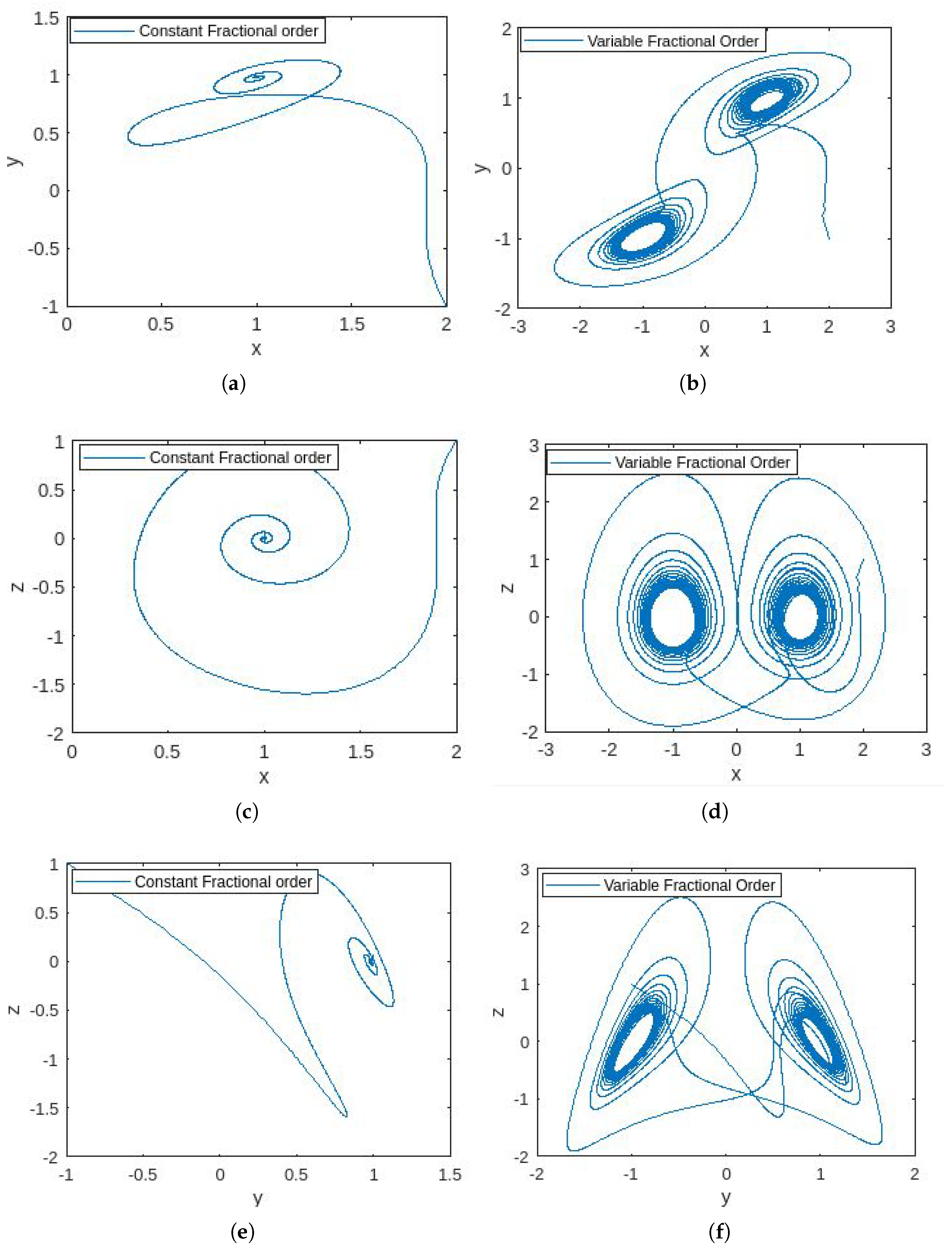
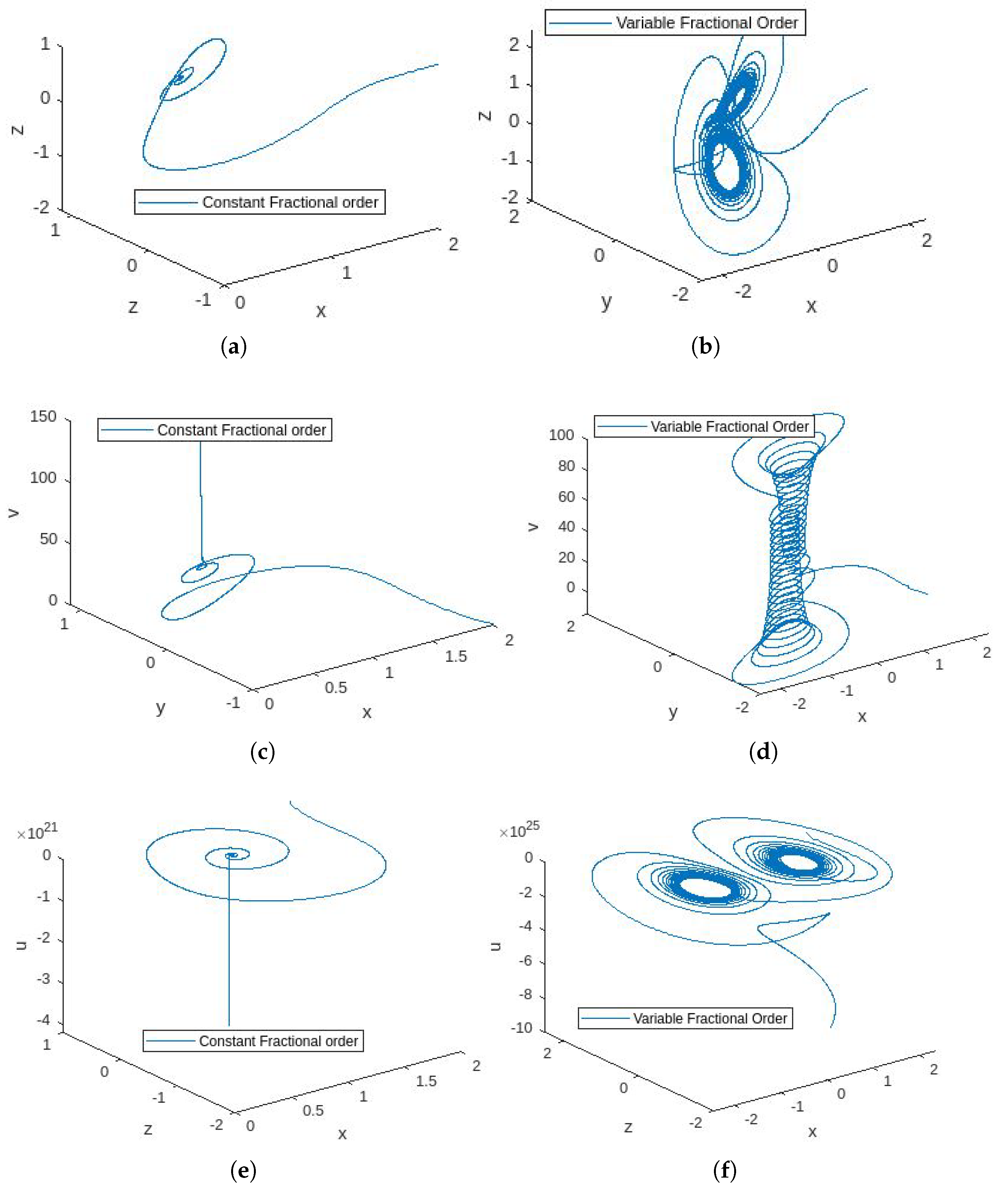
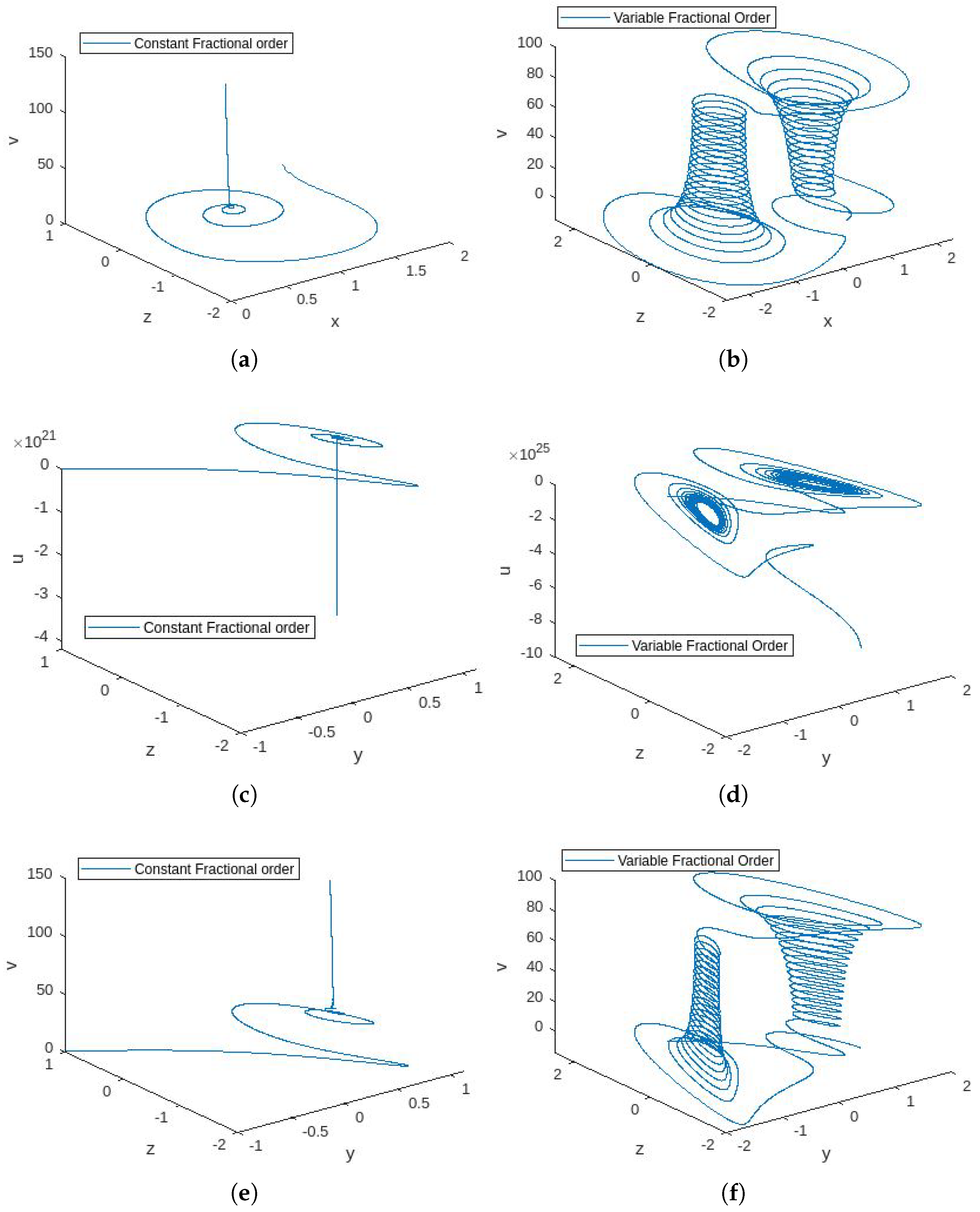
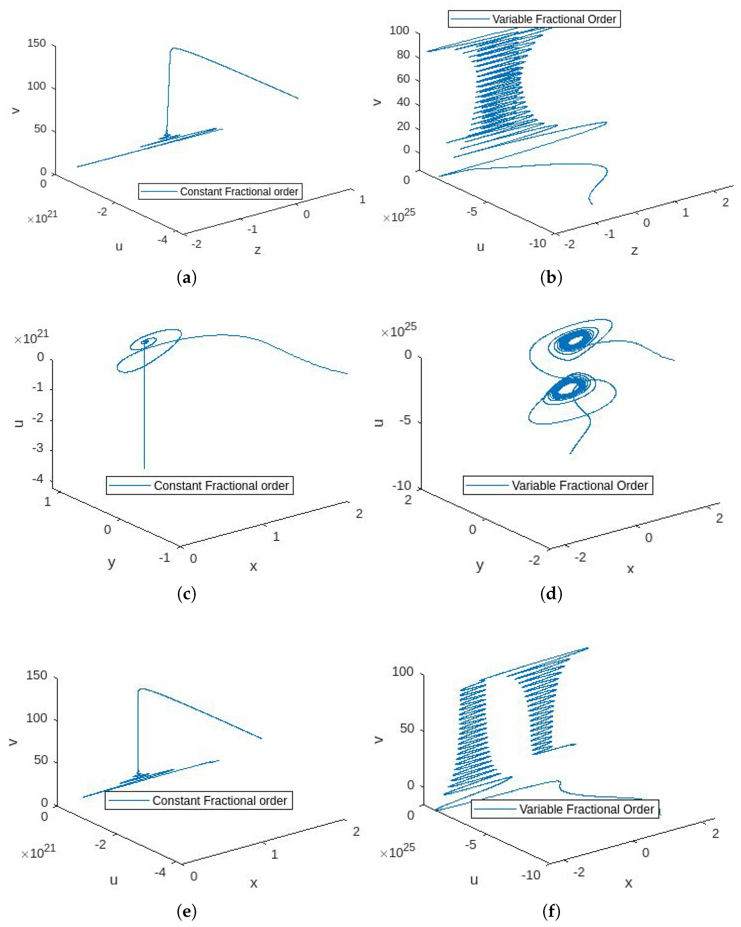
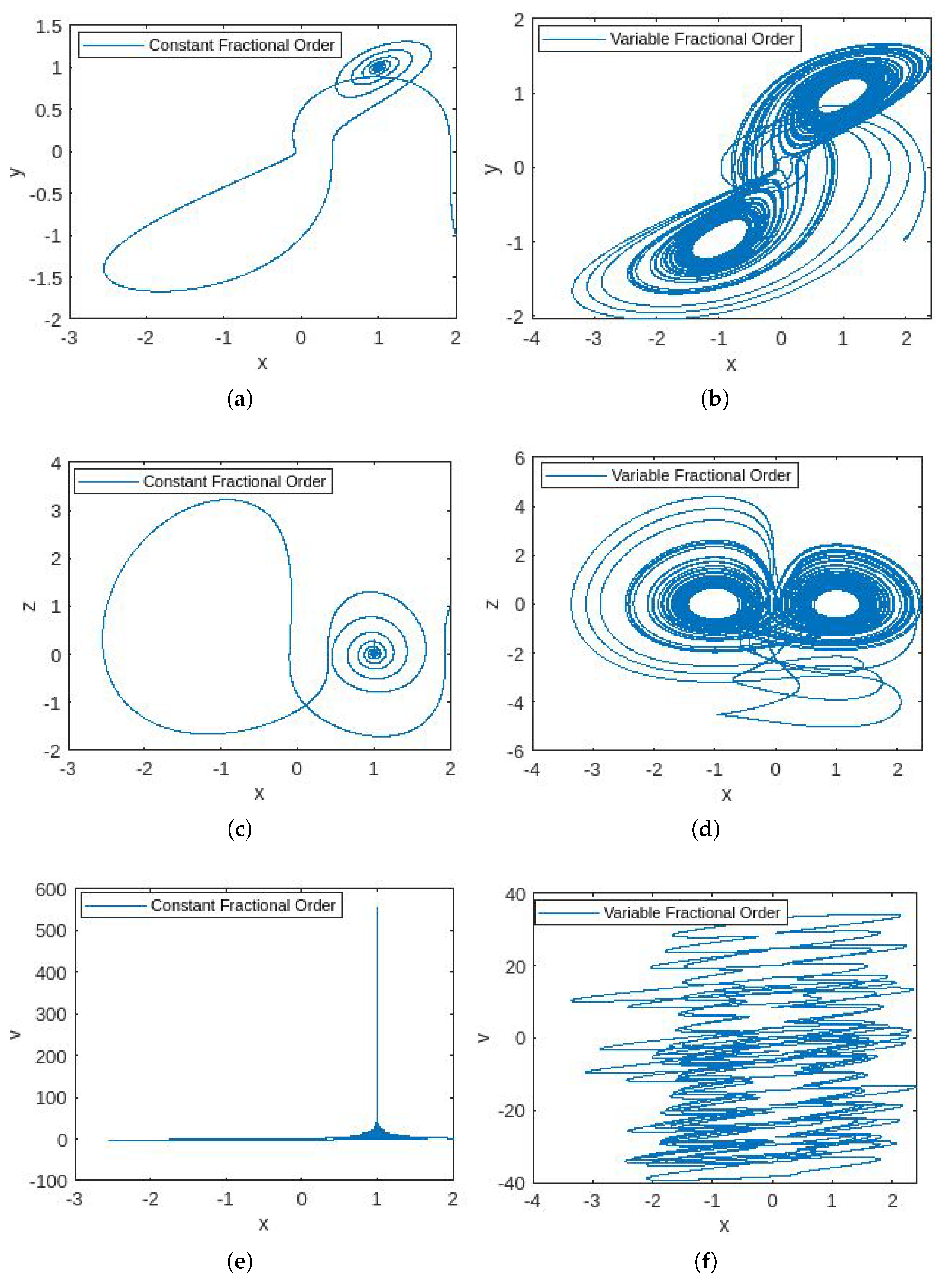
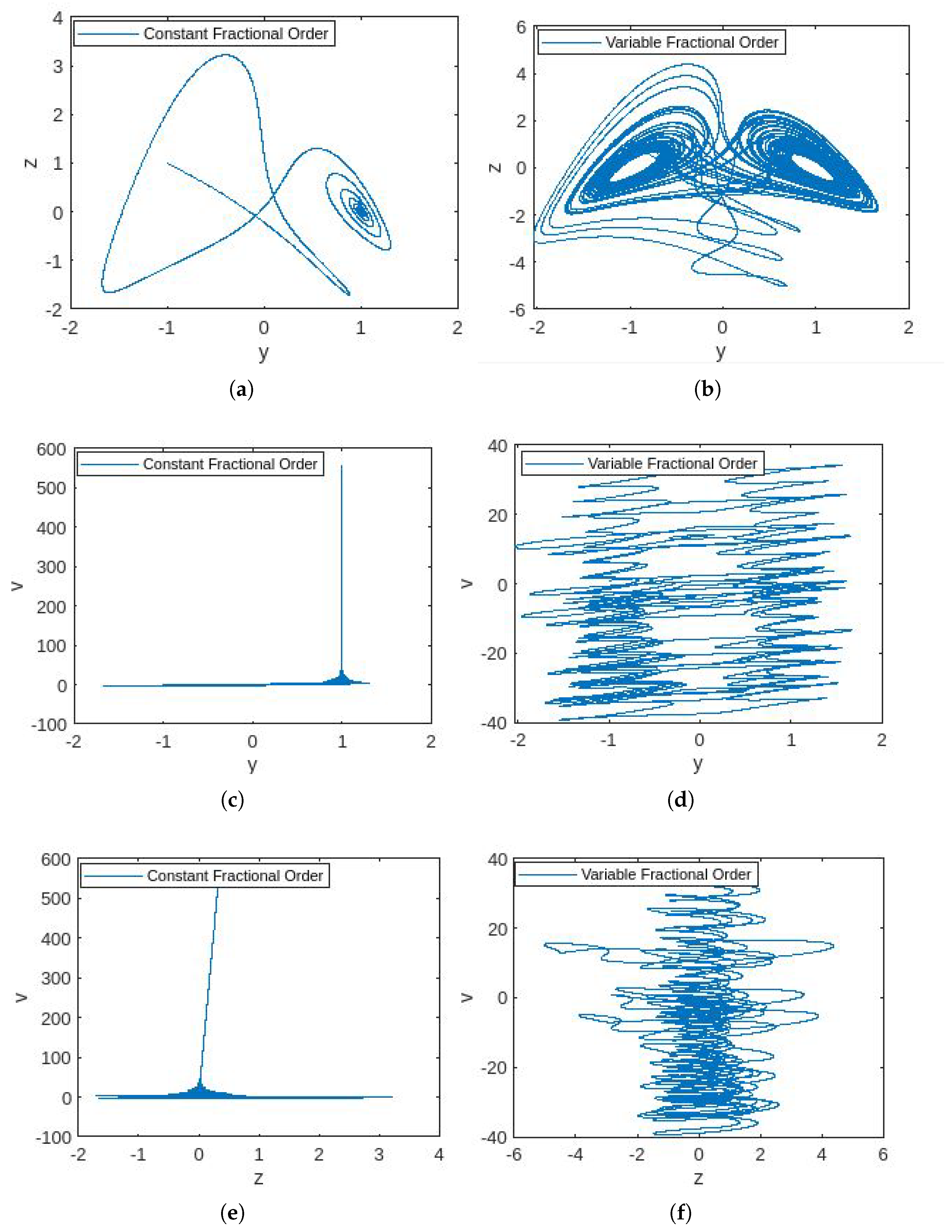
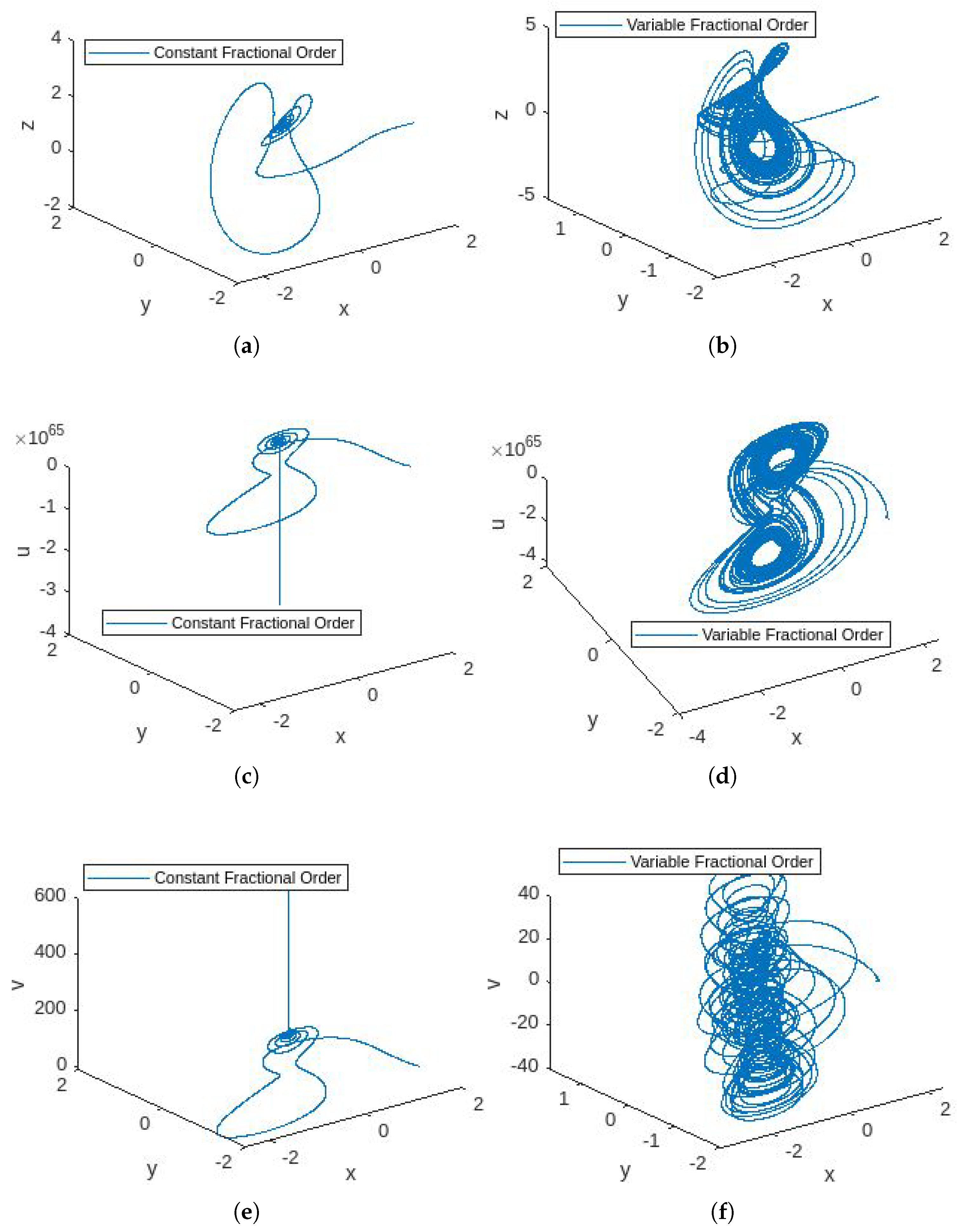
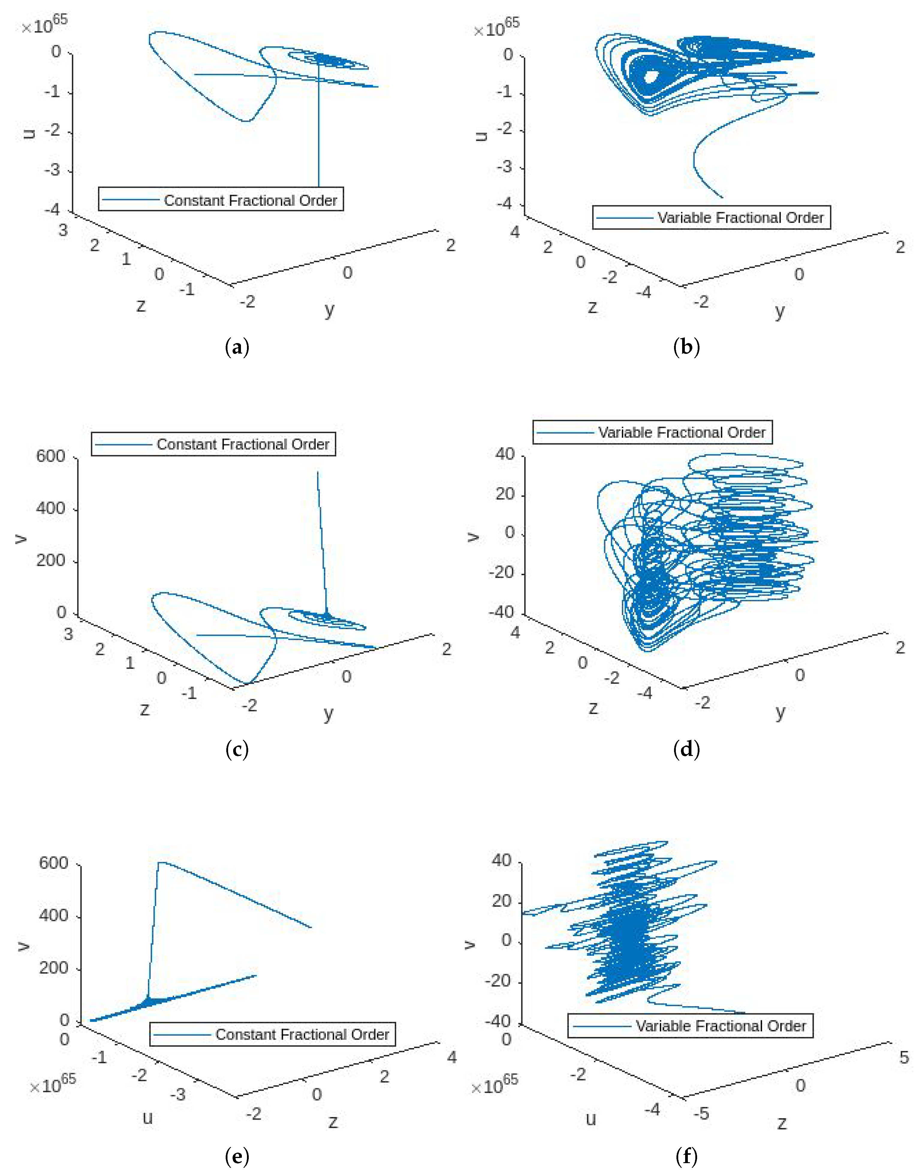
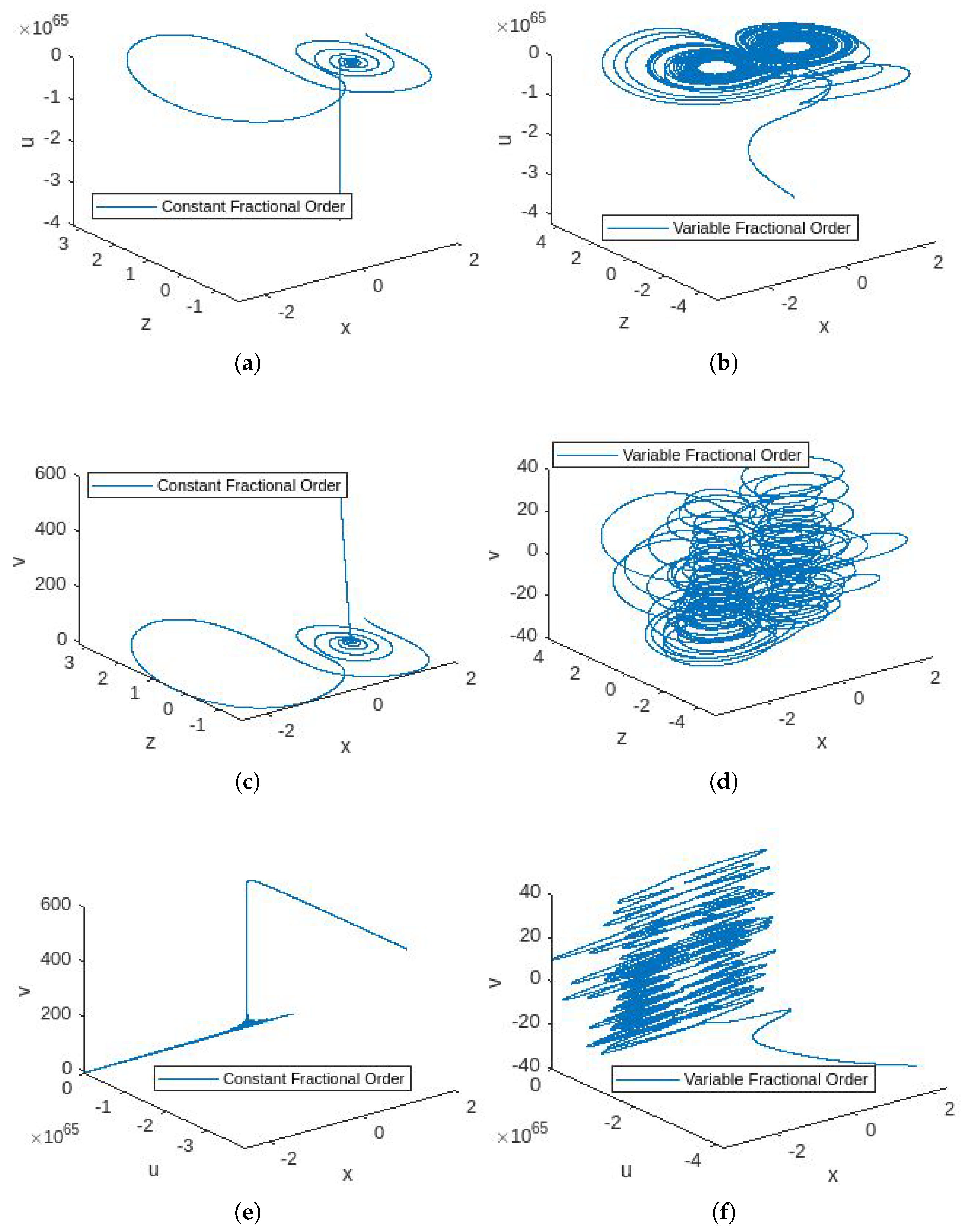
• In Figure 1, the phase portraits illustrating the behavior of the 5D constant- and variable-order fractional hyperchaotic systems with the Caputo derivative are presented.
• Figure 2, Figure 3 and Figure 4 present the 3D graphs used to illustrate the behavior of the 5D constant- and variable-order fractional hyperchaotic systems with Caputo derivative.
• In Figure 5 and Figure 6, the phase portraits illustrating the behavior of the 5D constant- and variable-order fractional hyperchaotic systems with the CF derivative are given.
• Figure 7, Figure 8 and Figure 9 present the 3D graphs illustrating the behavior of the constant- and variable-order fractional hyperchaotic systems with the CF derivative.

A difference can be observed between the dynamics of the behavior of the solution of the hyperchaotic system with constant order and the dynamics of the solution’s behavior with the variable order. We observe that when the order of the fractional derivative varies with respect to time, the intrinsic dynamics of the hyperchaotic system are captured more effectively as compared to the constant-order fractional hyperchaotic system. This shows that the variable-order hyperchaotic system provides a more comprehensive analysis and better understanding of the chaotic behavior of the system compared to the constant-order system.

Further, in Figure 1, Figure 2, Figure 3, Figure 4, Figure 5, Figure 6, Figure 7, Figure 8 and Figure 9, we can observe a difference in the chaotic behavior of the hyperchaotic system with two different fractional derivatives (Caputo and CF). We observe that due to the exponential kernel in the CF derivative, we see more complexity in the chaotic behaviour of the fractional hyperchaotic system with the CF derivative as compared to the fractional hyperchotic system with the Caputo derivative.

5. Conclusions

In this study, we examined both the constant- and variable-order fractional 5D hyperchaotic systems using the Caputo and CF derivatives. Numerical solutions for all four cases are presented in Section 3 and Section 4, along with the simulations. Figure 1, Figure 2, Figure 3 and Figure 4 show the chaotic behavior of the 5D constant- and variable-order Caputo fractional hyperchaotic systems at fractional order $\varrho =0.8999$. Figure 5, Figure 6, Figure 7, Figure 8 and Figure 9 illustrate the same for the CF fractional systems. By observing the figures, we conclude that the simulations highlight differences between constant- and variable-order Caputo and CF derivatives. Varying the fractional order with respect to t adds complexity to the chaotic behavior. As we examined the hyperchaotic system with two different fractional derivatives (Caputo and CF), our results demonstrate that the selection of fractional derivative markedly influences the chaotic behavior of the system. We observe that the CF derivative provides a more profound insight into the complexity of the 5D hyperchaotic system compared to the Caputo derivative. The exponential kernel in the CF derivative induces extensive interactions, leading to an intricate and unpredictable behavior. We also observe that hyperchaotic systems with a variable-order fractional derivative enable a more comprehensive analysis of the chaotic regions as compared to hyperchaotic systems with constant-order fractional derivatives. Hence, a hyperchaotic system with a variable-order fractional derivative deepens the understanding of the system’s dynamics.

References

1. Rossler, O.E. An equation for hyperchaos. Phys. Lett. A 1979, 71, 155–157. [Google Scholar] [CrossRef]
2. Erkan, U.; Toktas, A.; Lai, Q. 2D hyperchaotic system based on Schaffer function for image encryption. Expert Syst. Appl. 2023, 213, 119076. [Google Scholar] [CrossRef]
3. Erkan, U.; Toktas, A.; Lai, Q. Design of two dimensional hyperchaotic system through optimization benchmark function. Chaos Solitons Fractals 2023, 167, 113032. [Google Scholar] [CrossRef]
4. Zhu, S.; Deng, X.; Zhang, W.; Zhu, C. Construction of a new 2D hyperchaotic map with application in efficient pseudo-random number generator design and color image encryption. Mathematics 2023, 11, 3171. [Google Scholar] [CrossRef]
5. Gao, X. Image encryption algorithm based on 2D hyperchaotic map. Opt. Laser Technol. 2021, 142, 107252. [Google Scholar] [CrossRef]
6. Tang, J.; Zhang, Z.; Huang, T. Two-dimensional cosine–sine interleaved chaotic system for secure communication. IEEE Trans. Circuits Syst. II Express Briefs 2024, 71, 2479–2483. [Google Scholar] [CrossRef]
7. Tang, J.; Zhang, Z.; Chen, P.; Huang, Z.; Huang, T. A simple chaotic model with complex chaotic behaviors and its hardware implementation. IEEE Trans. Circuits Syst. I Regul. Pap. 2023, 70, 3676–3688. [Google Scholar] [CrossRef]
8. Li, W.; Yan, W.; Zhang, R.; Wang, C.; Ding, Q. A new 3D discrete hyperchaotic system and its application in secure transmission. Int. J. Bifurc. Chaos 2019, 29, 1950206. [Google Scholar] [CrossRef]
9. Huang, L.; Li, C.; Liu, J.; Zhong, Y.; Zhang, H. A novel 3D non-degenerate hyperchaotic map with ultra-wide parameter range and coexisting attractors periodic switching. Nonlinear Dyn. 2024, 112, 2289–2304. [Google Scholar] [CrossRef]
10. Cui, N.; Li, J. A new 4D hyperchaotic system and its control. AIMS Math. 2023, 8, 905–923. [Google Scholar] [CrossRef]
11. Leutcho, G.D.; Wang, H.; Fozin, T.F.; Sun, K.; Njitacke, Z.T.; Kengne, J. Dynamics of a new multistable 4D hyperchaotic Lorenz system and its applications. Int. J. Birfurc. Chaos 2022, 32, 2250001. [Google Scholar] [CrossRef]
12. Ojoniyi, O.S.; Njah, N.A. A 5D hyperchaotic Sprott B system with coexisting hidden attractors. Chaos Solitons Fractals 2016, 87, 172–181. [Google Scholar] [CrossRef]
13. Yu, F.; Liu, L.; Qian, S.; Li, L.; Huang, Y.; Shi, C.; Cai, S.; Wu, X.; Du, S.; Wan, Q. Chaos based application of a novel multistable 5D memristive hyperchaotic system with coexisting multiple attractors. Complexity 2020, 2020, 8034196. [Google Scholar] [CrossRef]
14. Li, J.; Cui, N. Dynamical analysis of a new 5D hyperchaotic system. Phys. Scr. 2023, 98, 105205. [Google Scholar] [CrossRef]
15. Liu, X.; Tong, X.; Zhang, M.; Wang, Z. A highly secure image encryption algorithm based on conservative hyperchaotic system and dynamic biogenetic gene algorithms. Chaos Solitons Fractals 2023, 171, 113450. [Google Scholar] [CrossRef]
16. Kocak, O.; Erkan, U.; Toktas, A.; Gao, S. PSO-based image encryption scheme using modular integrated logistic exponential map. Expert Syst. Appl. 2024, 237, 121452. [Google Scholar] [CrossRef]
17. Li, H.; Yu, S.; Feng, W.; Chen, Y.; Zhang, J.; Qin, Z.; Zhu, Z.; Wozniak, M. Exploiting dynamic vector-level operations and a 2D-enhanced logistic modular map for efficient chaotic image encryption. Entropy 2023, 25, 1147. [Google Scholar] [CrossRef] [PubMed]
18. Feng, W.; Zhao, X.; Zhang, J.; Qin, Z.; Zhang, J.; He, Y. Image encryption algorithm based on plane-level image filtering and discrete logarithmic transform. Mathematics 2022, 10, 2751. [Google Scholar] [CrossRef]
19. Wen, H.; Lin, Y. Cryptanalysis of an image encryption algorithm using quantum chaotic map and DNA coding. Expert Syst. Appl. 2024, 237, 121514. [Google Scholar] [CrossRef]
20. Nestor, T.; Belazi, A.; Abd-El-Atty, B.; Aslam, M.N.; Volos, C.; Dieu, N.J.D.; Abd-El-Latif, A.A. A new 4D hyperchaotic system with dynamics analysis, synchronization, and application to image encryption. Symmetry 2022, 14, 424. [Google Scholar] [CrossRef]
21. Wen, H.; Huang, Y.; Lin, Y. High-quality color image compression-encryption using chaos and block permutation. J. King Saud Univ.-Comput. Inf. Sci. 2023, 35, 101660. [Google Scholar] [CrossRef]
22. Hui, Y.; Liu, H.; Fang, P. A DNA image encryption based on a new hyperchaotic system. Multimed. Tools Appl. 2023, 82, 21983–22007. [Google Scholar] [CrossRef]
23. Benkouider, K.; Sambas, A.; Bonny, T.; Nassan, W.A.; Moghrabi, I.A.R.; Sulaiman, I.M.; Hassan, B.A.; Mamat, M. A comprehensive study of the novel 4D hyperchaotic system with self-exited multistability and application in the voice encryption. Sci. Rep. 2024, 14, 12993. [Google Scholar] [CrossRef] [PubMed]
24. Bonny, T.; Nassan, W.A.; Baba, A. Voice encryption using a unified hyper-chaotic system. Multimed. Tools Appl. 2023, 82, 1067–1085. [Google Scholar] [CrossRef]
25. Wen, H.; Lin, Y.; Xie, Z.; Liu, T. Chaos-based block permutation and dynamic sequence multiplexing for video encryption. Sci. Rep. 2023, 13, 14721. [Google Scholar] [CrossRef] [PubMed]
26. Naik, R.B.; Singh, U. A review on applications of chaotic maps in psuedo-random number generators and encryption. Ann. Data Sci. 2022, 11, 25–50. [Google Scholar] [CrossRef]
27. Bonny, T.; Debsi, R.A.; Majzoub, S.; Elwakil, A.S. Hardware optimized FPGA implementations of high-speed true random bit generators based on switching-type chaotic oscillators. Circuits Sys. Signal Process. 2019, 38, 1342–1359. [Google Scholar] [CrossRef]
28. Wong, K.-W.; Lin, Q.; Chen, J. Simultaneous arithmetic coding and encryption using chaotic maps. IEEE Trans. Circuits Sys. II Express Briefs 2010, 57, 146–150. [Google Scholar] [CrossRef]
29. Al-Kateeb, Z.N.; Mohammed, S.J. Encrypting an audio file based on integer wavelet transform and hand geometry. Telecommun. Comput. Electron. Control 2020, 18, 2012–2017. [Google Scholar] [CrossRef]
30. Oldham, K.B.; Spanier, J. The Fractional Calculus. Theory and Applications of Differentiation and Integration to Arbitrary Order; Academic Press: New York, NY, USA, 1974; p. 9780125255509. [Google Scholar]
31. Caputo, M.; Fabrizio, M. A new definition of fractional derivative without singular kernel, Prog. Fract.Differ. Appl. 2015, 1, 73–85. [Google Scholar]
32. Iskakova, K.; Alam, M.M.; Ahmad, S.; Saifullah, S.; Akgul, A.; Yılmaz, G. Dynamical study of a novel 4D hyperchaotic system: An integer and fractional order analysis. Math. Comput. Simul. 2023, 208, 219–245. [Google Scholar] [CrossRef]
33. Feng, W.; Wang, Q.; Liu, H.; Ren, Y.; Zhang, J.; Zhang, S.; Qian, K.; Wen, H. Exploiting newly designed fractional-order 3D lorenz chaotic system and 2D discrete polynomial hyper-chaotic map for high-performance multi-image encryption. Fractal Fract. 2023, 7, 887. [Google Scholar] [CrossRef]
34. Az-Zo’bi, E.A.; Alomari, Q.M.M.; Afef, K.; Inc, M. Dynamics of generalized time-fractional viscous-capillarity compressible fluid model. Opt. Quantum Electron. 2024, 56, 629. [Google Scholar] [CrossRef]
35. Sene, N. Theory and applications of new fractional-order chaotic system under Caputo operator. Int. J. Optim. Control Theor. Appl. 2022, 12, 20–38. [Google Scholar] [CrossRef]
36. Deng, H.; Li, T.; Wang, Q.; Li, H. A fractional-order hyperchaotic system and its synchronization. Chaos Solitons Fractals 2009, 41, 962–969. [Google Scholar] [CrossRef]
37. Balootaki, M.A.; Rahmani, H.; Moeinkhah, H.; Mohammadzadeh, A. On the synchronization and stabilization of fractional-order chaotic systems: Recent advances and future perspectives. Phys. A Stat. Mech. Appl. 2020, 551, 124203. [Google Scholar] [CrossRef]
38. Rahman, Z.A.S.A.; Jasim, B.H.; Al-Yasir, Y.I.A.; Hu, Y.F.; Alhameed, R.A.A.; Alhasnawi, B.N. A New Fractional-Order Chaotic System with Its Analysis, Synchronization, and Circuit Realization for Secure Communication Applications. Mathematics 2021, 20, 2593. [Google Scholar] [CrossRef]
39. Fuentes, O.M.; Garcia, J.J.M.; Aguilar, J.F.G. Generalized synchronization of commensurate fractional-order chaotic systems: Applications in secure information transmission. Digit. Signal Process. 2022, 126, 103494. [Google Scholar] [CrossRef]
40. Yang, F.; Mou, J.; Ma, C.; Cao, Y. Dynamic analysis of an improper fractional-order laser chaotic system and its image encryption application. Opt. Lasers Eng. 2020, 129, 106031. [Google Scholar] [CrossRef]
41. Mohamed, S.M.; Sayed, W.S.; Madian, A.H.; Radwan, A.G.; Said, L.A. An Encryption Application and FPGA Realization of a Fractional Memristive Chaotic System. Electronics 2023, 12, 1219. [Google Scholar] [CrossRef]
42. Xu, S.; Wang, X.; Ye, X. A new fractional-order chaos system of Hopfield neural network and its application in image processing. Chaos Solitons Fractals 2022, 157, 111889. [Google Scholar] [CrossRef]
43. Chen, L.; Yin, H.; Huang, T.; Yuan, L.; Zheng, S.; Yin, L. Chaos in fractional-order discrete neural networks with application to image encryption. Neural Netw. 2020, 125, 174–184. [Google Scholar] [CrossRef] [PubMed]
44. Azzawi, S.F.A.; Hasan, A.M. New 5D Hyperchaotic system derived from the Sprott C system: Properties and Anti Synchronization. J. Intell. Syst. Control 2023, 2, 110–122. [Google Scholar] [CrossRef]
45. Samko, S. Fractional integration and differentiation of variable order: An overview. Nonlinear Dyn. 2013, 71, 653–662. [Google Scholar] [CrossRef]
46. Yousefpour, A.; Jahanshahi, H.; Castillo, O. Application of variable-order fractional calculus in neural networks: Where do we stand? Eur. Phys. J. Spec. Top. 2022, 231, 1753–1756. [Google Scholar] [CrossRef]
47. Moghaddam, B.P.; Dabiri, A.; Machado, J.A.T. Application of variable-order fractional calculus in solid mechanics. Appl. Eng. Life Soc. Sci. Part A 2019, 7, 207–224. [Google Scholar] [CrossRef]
48. Patnaik, S.; Semperlotti, F. Application of variable- and distributed-order fractional operators to the dynamic analysis of nonlinear oscillators. Nonlinear Dyn. 2020, 100, 561–580. [Google Scholar] [CrossRef]
49. Perez, J.E.S.; Aguilar, J.F.G.; Atangana, A. Novel numerical method for solving variable-order fractional differential equations with power, exponential and Mittag-Leffler laws. Chaos Solitons Fractals 2018, 114, 175–185. [Google Scholar] [CrossRef]
50. Butt, A.I.K.; Ahmad, W.; Rafiq, M.; Baleanu, D. Numerical analysis of Atangana-Baleanu fractional model to understand the propagation of a novel corona virus pandemic. Alex. Eng. J. 2022, 61, 7007–7027. [Google Scholar] [CrossRef]
51. Toufik, M.; Atangana, A. Correction to: New numerical approximation of fractional derivative with non-local and non-singular kernel: Application to chaotic models. Eur. Phys. J. Plus. 2022, 137, 191. [Google Scholar] [CrossRef]
Figure 1. Comparison between the phase portrait behavior of constant- and variable-order fractional Caputo 5D hyperchaotic systems with ϱ = 0.899 , a = 1 , b = 0.3 , c = 0.006 , p = 1 , x ( 0 ) = 0.1 , y ( 0 ) = 0.1 , z ( 0 ) = 0.2 , u ( 0 ) = 0.1 , and v ( 0 ) = 0.2 : (a) x-y plane phase portrait at constant fractional order 0.899; (b) x-y plane phase portrait at variable fractional order 0.899; (c) x-z plane phase portrait at constant fractional order 0.899; (d) x-z plane phase portrait at variable fractional order 0.899; (e) y-z plane phase portrait at constant fractional order 0.899; (f) y-z plane phase portrait at variable fractional order 0.899.
Fractalfract 08 00421 g001
Figure 2. Three-dimensional graphs showing a comparison between constant- and variable-order fractional Caputo 5D hyperchaotic systems with ϱ = 0.899 , a = 1 , b = 0.3 , c = 0.006 , p = 1 , x ( 0 ) = 0.1 , y ( 0 ) = 0.1 , z ( 0 ) = 0.2 , u ( 0 ) = 0.1 , and v ( 0 ) = 0.2 : (a) x-y-z plane representation at constant fractional order 0.899; (b) x-y-z plane representation at variable fractional order 0.899; (c) x-y-v plane representation at constant fractional order 0.899; (d) x-y-v plane representation at variable fractional order 0.899; (e) x-z-u plane representation at constant fractional order 0.899; (f) x-z-u plane representation at variable fractional order 0.899.
Fractalfract 08 00421 g002
Figure 3. Three-dimensional graphs showing a comparison between constant- and variable-order fractional Caputo 5D hyperchaotic systems with ϱ = 0.899 , a = 1 , b = 0.3 , c = 0.006 , p = 1 , x ( 0 ) = 0.1 , y ( 0 ) = 0.1 , z ( 0 ) = 0.2 , u ( 0 ) = 0.1 , and v ( 0 ) = 0.2 : (a) x-z-v plane representation for constant-order Caputo derivative; (b) x-z-v plane representation for variable-order Caputo derivative; (c) y-z-u plane representation for constant-order Caputo derivative; (d) y-z-u plane representation for variable-order Caputo derivative; (e) y-z-v plane representation for constant-order Caputo derivative; (f) y-z-v plane representation for variable-order Caputo derivative.
Fractalfract 08 00421 g003
Figure 4. Three-dimensional graphs showing a comparison between constant- and variable-order fractional Caputo 5D hyperchaotic systems with ϱ = 0.899 , a = 1 , b = 0.3 , c = 0.006 , p = 1 , x ( 0 ) = 0.1 , y ( 0 ) = 0.1 , z ( 0 ) = 0.2 , u ( 0 ) = 0.1 , and v ( 0 ) = 0.2 : (a) z-u-v plane representation for constant-order Caputo derivative; (b) z-u-v representation for variable-order Caputo derivative; (c) x-y-u representation for constant-order Caputo derivative; (d) x-y-u representation for variable-order Caputo derivative; (e) x-u-v representation for constant-order Caputo derivative; (f) x-u-v representation for variable-order Caputo derivative.
Fractalfract 08 00421 g004
Figure 5. Comparison between the phase portraits of constant- and variable-order fractional CF 5D hyperchaotic systems with ϱ = 0.899 , a = 1 , b = 0.3 , c = 0.006 , p = 1 , x ( 0 ) = 0.1 , y ( 0 ) = 0.1 , z ( 0 ) = 0.2 , u ( 0 ) = 0.1 , and v ( 0 ) = 0.2 : (a) x-y plane phase portrait at constant fractional order 0.899; (b) x-y plane phase portrait at variable fractional order 0.899; (c) x-z plane phase portrait at constant fractional order 0.899; (d) x-z plane phase portrait at variable fractional order 0.899; (e) x-v plane phase portrait at constant fractional order 0.899; (f) x-v plane phase portrait at variable fractional order 0.899.
Fractalfract 08 00421 g005
Figure 6. Comparison between the phase portraits of constant- and variable-order fractional CF 5D hyperchaotic systems with ϱ = 0.899 , a = 1 , b = 0.3 , c = 0.006 , p = 1 , x ( 0 ) = 0.1 , y ( 0 ) = 0.1 , z ( 0 ) = 0.2 , u ( 0 ) = 0.1 , and v ( 0 ) = 0.2 : (a) y-z plane phase portrait at constant fractional order 0.899; (b) y-z plane phase portrait at variable fractional order 0.899; (c) y-v plane phase portrait at constant fractional order 0.899; (d) y-z plane phase portrait at variable fractional order 0.899; (e) z-v plane phase portrait at constant fractional order 0.899; (f) z-v plane phase portrait at variable fractional order 0.899.
Fractalfract 08 00421 g006
Figure 7. Three-dimensional graphs showing a comparison between constant- and variable-order fractional CF 5D hyperchaotic systems with ϱ = 0.899 , a = 1 , b = 0.3 , c = 0.006 , p = 1 , x ( 0 ) = 0.1 , y ( 0 ) = 0.1 , z ( 0 ) = 0.2 , u ( 0 ) = 0.1 , and v ( 0 ) = 0.2 : (a) x-y-z representation for constant-order CF derivative; (b) x-y-z representation for variable-order CF derivative; (c) x-y-u representation for constant-order CF derivative; (d) x-y-u representation for variable-order CF derivative; (e) x-y-v representation for constant-order CF derivative; (f) x-y-v representation for variable-order CF derivative.
Fractalfract 08 00421 g007
Figure 8. Three-dimensional graphs showing a comparison between constant- and variable-order fractional CF 5D hyperchaotic systems with ϱ = 0.899 , a = 1 , b = 0.3 , c = 0.006 , p = 1 , x ( 0 ) = 0.1 , y ( 0 ) = 0.1 , z ( 0 ) = 0.2 , u ( 0 ) = 0.1 , and v ( 0 ) = 0.2 : (a) y-z-u representation for constant-order CF derivative; (b) y-z-u representation for variable-order CF derivative; (c) y-z-v representation for constant-order CF derivative; (d) y-z-v representation for variable-order CF derivative; (e) z-u-v representation for constant-order CF derivative; (f) z-u-v representation for variable-order CF derivative.
Fractalfract 08 00421 g008
Figure 9. Three-dimensional graphs showing a comparison between constant- and variable-order fractional CF 5D hyperchaotic systems with ϱ = 0.899 , a = 1 , b = 0.3 , c = 0.006 , p = 1 , x ( 0 ) = 0.1 , y ( 0 ) = 0.1 , z ( 0 ) = 0.2 , u ( 0 ) = 0.1 , and v ( 0 ) = 0.2 : (a) x-z-u representation for constant-order CF derivative; (b) x-z-u representation for variable-order CF derivative; (c) x-z-v representation for constant-order CF derivative; (d) x-z-v representation for variable-order CF derivative; (e) x-u-v representation for constant-order CF derivative; (f) x-u-v representation for variable-order CF derivative.
Fractalfract 08 00421 g009
Disclaimer/Publisher’s Note: The statements, opinions and data contained in all publications are solely those of the individual author(s) and contributor(s) and not of MDPI and/or the editor(s). MDPI and/or the editor(s) disclaim responsibility for any injury to people or property resulting from any ideas, methods, instructions or products referred to in the content.