Abstract
In this paper, by replacing the exponential memory kernel function of a tabu learning single-neuron model with the power-law memory kernel function, a novel Caputo’s fractional-order tabu learning single-neuron model and a network of two interacting fractional-order tabu learning neurons are constructed firstly. Different from the integer-order tabu learning model, the order of the fractional-order derivative is used to measure the neuron’s memory decay rate and then the stabilities of the models are evaluated by the eigenvalues of the Jacobian matrix at the equilibrium point of the fractional-order models. By choosing the memory decay rate (or the order of the fractional-order derivative) as the bifurcation parameter, it is proved that Hopf bifurcation occurs in the fractional-order tabu learning single-neuron model where the value of bifurcation point in the fractional-order model is smaller than the integer-order model’s. By numerical simulations, it is shown that the fractional-order network with a lower memory decay rate is capable of producing tangent bifurcation as the learning rate increases from 0 to 0.4. When the learning rate is fixed and the memory decay increases, the fractional-order network enters into frequency synchronization firstly and then enters into amplitude synchronization. During the synchronization process, the oscillation frequency of the fractional-order tabu learning two-neuron network increases with an increase in the memory decay rate. This implies that the higher the memory decay rate of neurons, the higher the learning frequency will be.
1. Introduction
The human brain is a network connected by billions of neurons through synapses. Excited by external stimuli, the response of the brain is transmitted through the network in the form of electrical signals. It is therefore of significant importance to study neurons firing to disclose the function of the brain. To date, based on plenty of experiments and the experimental data, many classical neuron models have been constructed, such as the Hodgkin–Huxley (H-H) model [1,2], FitzHugh–Nagumo (FHN) model [3,4,5], Morris–Lecar (ML)model [6,7], Hindmarsh–Rose (HR) model [8,9], Chay model [10], Rulkov model [11], and Izhikevich model [12]. These models can emulate different neurons and display different neurodynamics, such as resting states, periodic oscillations, and chaos. The different neurodynamics, as mentioned earlier, play important roles in neural information encoding.
Tabu learning is the method of applying tabu search in neural networks to solve optimization problems [13]. Based on the energy distribution around the current state, tabu learning can avoid searched states and find new ones that are not searched, and then the search efficiency can be improved. In tabu learning searches, the neurons need some judgment and selection. This implies that the tabu learning neuron owns the memory. In existing models about tabu learning, the memory is described by the integration of state variable [13,14].
Tabu learning single-neuron models are two-dimensional [13] and are studied widely because of their simple mathematical structure [14,15,16,17,18,19,20,21]. Choosing the memory decay rate as the bifurcation parameter, Hopf bifurcations are shown in tabu learning neurons [14,15,17,19]. In [20], by replacing the resistive self-connection synaptic weight with a memristive self-connection synaptic weight, a memristive synaptic weight-based tabu learning neuron model is proposed. In the memristive synaptic weight-based tabu learning neuron model, there are infinitely many nonchaotic attractors composed of mono-periodic, multi-periodic, and quasi-periodic orbits. Additionally, in [18], hidden attractors are discovered in a non-autonomous tabu learning model with sinusoidal external excitation. Recently, based on the sinusoidal activation function, reference [21] proposed a two-dimensional non-autonomous tabu learning single-neuron model which can generate a class of multi-scroll chaotic attractors with parameters controlling the number of scrolls.
In the tabu learning single neuron models mentioned above, the exponential memory kernel function is applied. Compared to the power-law memory kernel function , the exponential memory kernel function limits to zero more quickly as . Therefore, the exponential memory kernel function results in a lower memory capacity for the states. As stated in [22], memory capacity is limited if the memory states are not truly persistent over time. For improving memory capacity, it is reasonable to replace the exponential memory kernel function of the neuron by the power-law memory kernel function. In fact, the fractional-order derivative is defined in the power-law memory kernel function. And it has been proven that the fractional-order derivative owns the memory effect and is not a strictly local operator [23]. The order of the fractional-order derivative is related to the memory loss or the “proximity effect” of some characteristics [24]. Then, in the following discussion, the exponential memory kernel function of the neuron was replaced by the power-law memory kernel function, and a novel Caputo’s fractional-order tabu learning single-neuron model and a network of two interacting Caputo fractional-order tabu learning neurons are proposed. In these new fractional-order models, the physical meaning of the order of the fractional-order derivatives is the memory decay rate of the neuron.
To begin with, by choosing the memory decay rate (i.e., the order of the fractional-order derivative) as a bifurcation parameter, it is proved that Hopf bifurcation occurs in the Caputo’s fractional-order tabu leaning single-neuron model. Secondly, the dynamics of the network of two interacting Caputo’s fractional-order tabu learning neurons is discussed. With a lower memory decay rate, the fractional-order network showed tangent bifurcation as the learning rate increased from 0 to 0.4. Then, when the learning rate was fixed, the network entered into frequency synchronization firstly and then the amplitudes of two neurons gradually became consistent as the memory decay rate increased from 0 to 1. This study shows that the memory decay rate, i.e., the order of the fractional-order derivative, has a significant impact on the dynamics of fractional-order tabu learning neuron models.
The paper is organized as follows. The Caputo’s fractional-order tabu learning single-neuron model and the network of two interacting Caputo’s fractional-order tabu learning neurons are proposed in Section 2. In Section 3, the stabilities of the models are evaluated by the eigenvalues of the Jacobian matrix at the equilibrium point. In Section 4, numerical simulations of the fractional-order models are shown. Finally, conclusions are drawn in Section 5.
2. Preliminaries and Fractional-Order Tabu Learning Models
2.1. Preliminaries on Fractional-Order Systems
First, the -order (0 < < 1) integral is defined by [23] as
where is the Gamma function. Corresponding to the fractional-order integral, there is a fractional-order derivative which has several different definitions such as Grunwald–Letnikov’s derivative, Caputo’s derivative, and Riemann-Liouville’s derivative. In this study, Caputo’s derivative is employed. The -order () derivative is defined as
where is the first-order derivative of function . The integration in Equation (2) indicates that the Caputo’s derivative is non-local. Consequently, a fractional-order mathematical model can contain the memory of system variables.
For the stability analysis of a fractional-order mathematical model, the following lemma is needed [25].
Lemma 1.
The fractional-order system
is asymptotically stable at the equilibrium point if all the eigenvalues λ of the Jacobian matrix satisfy the condition:
where is the argument of λ, , and , .
2.2. A Fractional-Order Tabu Learning Single-Neuron Model
A classical tabu learning single-neuron model is described by [15] as
where u is the action potential of the neuron, J is the tabu learning variable, is the activation function, and a is the self-connection strength of the neuron. In model (5), the tabu learning variable J is computed by
where is the memory decay rate and is the learning rate. As , the exponential memory kernel function limits to zero more quickly than the power-law memory kernel function . That is to say, with the exponential memory kernel function , the memory capacity of the neuron is not truly persistent over time and so neurons will begin to relearn states that have been learned but forgotten. To make the memory time long enough, the exponential kernel function in Equation (6) is replaced by the power-law kernel function . By doing so, the tabu learning variable J is computed by
Equation (7) can be rewritten as
Referring to Equation (1), the tabu learning variable J can be described as
Based on the following relationship,
we can obtain
Then, a novel fractional-order tabu learning single neuron model is proposed as follows:
where is the memory decay rate and is the learning rate.
2.3. A Fractional-Order Coupled Tabu Learning Two-Neuron Model
In this section, a network of two interacting fractional-order tabu learning neurons with the lower memory decay rate is constructed as follows:
where the learning rate is changed in the interval , the activation function , and the weight matrix Q between two neurons is
The classical integer-order model corresponding to model (13) is displayed in [15].
3. Dynamics of the Fractional-Order Models
3.1. Stability Analysis of Model (12)
If has the root of , model (12) has an equilibrium point . The Jacobian matrix M at E is
The characteristic equation of matrix M is
where . The eigenvalues of matrix M are
The eigenvalues changed with the parameters are displayed in Table 1, where is the real part of the eigenvalue .

Table 1.
The eigenvalue .
Remark 1. (1) If ( is the imaginary part of λ), λ is a real number. As , one has ; as , one has .
- (2) If , it is easy to know . Then as , one has ; as , one has .
By the location of eigenvalue on the complex plain, the stability of model (12) can be evaluated as following:
As , shown in Table 1, two eigenvalues are real numbers and one of them is in the positive real axis of the complex plane, i.e., there is . So as , model (12) at the equilibrium point E is unstable for any .
As , due to and , one has . Thus, , and . So, as , model (12) at the equilibrium point E is stable.
As and , two eigenvalues are negative real numbers. And . In this case, model (12) at the equilibrium point E is stable.
As and , two eigenvalues are positive real numbers. Then, . Model (12) at the equilibrium point E is unstable.
As and , both eigenvalues have positive real parts. The argument of the eigenvalue is . Referring to Lemma 1, model (12) at the equilibrium point E is stable if and is unstable if .
- Therefore, the following conclusions can be drawn:
Theorem 1.
The stability of model (12) at the equilibrium E depends on the parameters and . It is stated as:
3.2. Stabilty Analysis of Model (13) with the Decay Rate
The Jacobian matrix corresponding to model (13) at the equilibrium point is
Thus, the eigenpolynomial for discriminating the stability of equilibrium point can be yielded as
where . Due to , is not the root of Equation (17). Then, Equation (17) can be changed into
Thus,
When substituting into Equation (19), we obtain
where . Furthermore, we can obtain
Then, the roots of Equation (17) are
If and , the eigenvalues .
- If and , there are
- Due to , with and , we obtain
4. Numerical Simulations of the Fraction-Order Models
4.1. Numerical Simulations of Model (12)
In this section, the numerical simulations of model (12) are shown with . In this case, the equilibrium , and . As , one has and . Referring to Theorem 1, the bifurcation point can be calculated by
By using Matlab, Equation (23) has the root . Figure 1 is the time history of the action potential u. As , the action potential u is periodic spiking; while , the action potential u convergences to the quiescent state. These numerical results are consistent with the third conclusion shown in Theorem 1.
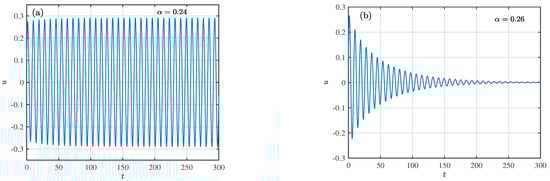
Figure 1.
The time history of u. (a) ; (b) .
Remark 2.
It is shown in [15] that model (5) shows Hopf Bifurcation when the memory decay rate , while in the fractional-order model (12), Hopf Bifurcation occurs when the memory decay rate . This implies that the memory kernel function has heavy effects on the dynamics of the tabu learning single-neuron model.
4.2. Dynamics of Model (13) with Induced by the Learning Rate
As shown in Section 3.2, model (13) is unstable for all . In this case, periodic spiking and chaotic spiking occur in model (13). Figure 2 is the bifurcation diagram of the local maxima of the variable . It is found that model (13) changes between the periodic spiking and the chaotic spiking as increases from 0 to 0.4. While , model (13) goes into chaotic spiking. Figure 3 is the time history of state for different values. There is periodic spiking when , , and , and then there is chaotic spiking when , , , , and . This implies that model (13) shows that tangent bifurcation increased from 0 to 0.4 and shows only chaotic spiking when .
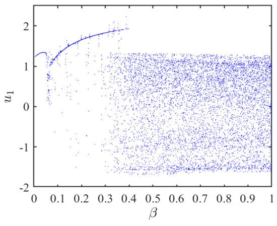
Figure 2.
Bifurcation diagram of the local maxima of the variable of model (13) regarding .
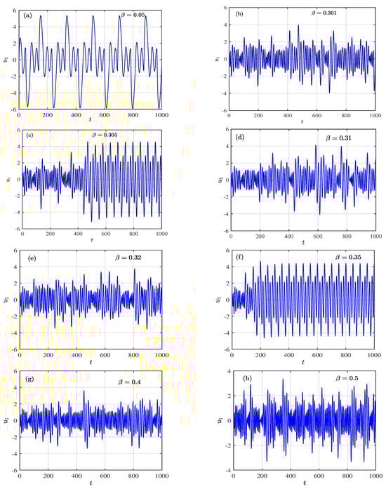
Figure 3.
The time history of . (a) ; (b) ; (c) ; (d) ; (e) ; (f) ; (g) ; (h) .
4.3. Dynamic Transitions of Model (13) Induced by the Memory Decay Rate
In Section 4.1, model (12) with different memory decay rates shows different dynamics. Taking this into account, we chose a different memory decay rate for model (13) with .
When and , model (13) is chaotic (Figure 4a1,b1). When or , model (13) goes into periodic spiking (Figure 4c1,d1), and it is found that the frequency of the oscillation increases as the order increases. This implies that the learning frequency of tabu learning neurons is very high when the memory decay rate is high. In theory, this is quite consistent with the actual phenomenon. In addition, when the memory decay rate increased from 0.01 to 0.9, Figure 4a2,b2,c2,d2 show that model (13) enters frequency synchronization firstly and then the amplitudes of two neurons gradually become consistent. This implies that the memory decay rate has a significant impact on the synchronization of the neurons connected by model (13).
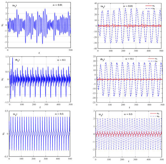
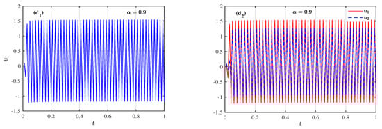
Figure 4.
The time histories of model (13): (a1–c1,d1) are the time histories of ; (a2–d2) are the time histories of and .
Remark 3.
When , the classical integer-order model with the memory decay rate corresponding to model (13) produces periodic spiking [15], while the fractional-order model (13) with shows chaotic spiking (Figure 4b2). The conclusion is drawn that the fractional-order model (13) has stronger nonlinearity than the corresponding classical integer-order model.
5. Conclusions
In this paper, a novel fractional-order tabu learning single-neuron mathematical model is proposed by introducing the exponential memory kernel function to the tabu learning variable. In the new model, the memory decay rate is measured by the order of the fractional-order derivative. Similar to the integer-order tabu learning neuron, the fractional-order tabu learning neuron model showed Hopf bifurcation as the memory decay rate increased from 0 to 1. It is interesting that the memory decay rate at which the fractional-order model showed Hopf bifurcation is numerically smaller than that of the integer-order tabu learning model. This indicates that the memory capacity has a significant impact on the neuron behavior. Based on this new fractional-order tabu learning model, the network of two interacting fractional-order tabu learning neurons is displayed. It is found that the network with a lower memory decay rate of 0.01 is unstable and shows tangent bifurcation as the learning rate increases from 0 to 1. However, when fixing the learning rate at 0.5 and increasing the memory decay from 0 to 1, the network enters into frequency synchronization firstly and then the amplitudes of two neurons gradually become consistent. At the same time, the numerical simulation shows that the bigger the memory decay rate is, the higher the learning frequency of the fractional-order tabu learning neuron network is, which coincides with the rule of fast forgetting and fast learning. This indicates that the memory decay rate takes an important role in the synchronization of a network connected by two fractional-order tabu learning neurons.
Of course, all results stated above are based only on mathematical models and theoretical analysis. In future research, it is needed to confirm that the actual firing of neurons matches our model.
Author Contributions
Conceptualization, Y.Y. and F.W.; methodology, Y.Y.; software, M.S.; validation, Z.G.; formal analysis, Y.Y.; investigation, Y.Y.; writing—original draft preparation, Y.Y.; supervision, F.W. All authors have read and agreed to the published version of the manuscript.
Funding
This research was supported by the grants from the National Natural Science Foundation of China under 11602035, 12172066, the Natural Science Foundation of Jiangsu Province, China under BK20201447, and the Science and Technology Innovation Talent Support Project of Jiangsu Advanced Catalysis and Green Manufacturing Collaborative Innovation Center under ACGM2022-10-02.
Data Availability Statement
All data were contained in the main text.
Conflicts of Interest
The authors declare no conflicts of interest.
References
- Hodgkin, A.; Huxley, A. A quantitative description of membrane current and its application to conduction and excitation in nerve. J. Physiol. 1952, 117, 500–544. [Google Scholar] [CrossRef] [PubMed]
- Xu, Q.; Wang, Y.; Chen, B.; Li, Z.; Wang, N. Firing pattern in a memristive Hodgkin-Huxley circuit: Numerical simulation and analog circuit validation. Chaos Solitons Fractals 2023, 172, 113627. [Google Scholar] [CrossRef]
- Nagumo, J.; Arimoto, S.; Yoshizawa, S. An Active Pulse Transmission Line Simulating Nerve Axon. Proc. IRE 1962, 50, 2061–2070. [Google Scholar] [CrossRef]
- Njitacke, Z.T.; Ramadoss, J.; Takembo, C.N.; Rajagopal, K.; Awrejcewicz, J. An enhanced FitzHugh–Nagumo neuron circuit, microcontroller-based hardware implementation: Light illumination and magnetic field effects on information patterns. Chaos Solitons Fractals 2023, 167, 113014. [Google Scholar] [CrossRef]
- Yao, Z.; Sun, K.; He, S. Firing patterns in a fractional-order FithzHugh-Nagumo neuron model. Nonlinear Dyn. 2022, 110, 1807–1822. [Google Scholar] [CrossRef]
- Morris, C.; Lecar, H. Voltage oscillations in the barnacle giant muscle fiber. Biophys. J. 1981, 35, 193–213. [Google Scholar] [CrossRef]
- Fan, W.; Chen, X.; Wu, H.; Li, Z.; Xu, Q. Firing patterns and synchronization of Morris-Lecar neuron model with memristive autapse. Int. J. Electron. Commun. (AEÜ) 2023, 158, 154454. [Google Scholar] [CrossRef]
- Hindmarsh, J.; Rose, M. A model of neuronal bursting using three coupled first order differential equations. Proc. R. Soc. B 1984, 221, 87–102. [Google Scholar]
- Xie, Y.; Yao, Z.; Ren, G.; Ma, J. Estimate physical reliability in Hindmarsh-Rose neuron. Phys. Lett. A 2023, 464, 128693. [Google Scholar] [CrossRef]
- Chay, T.R. Chaos in a three-variable model of an excitable cell. Physica D 1985, 16, 233–242. [Google Scholar] [CrossRef]
- Bao, H.; Li, K.; Ma, J.; Hua, Z.; Xu, Q.; Bao, B. Memristive effects on an improved discrete Rulkov neuron model. Sci. China Technol. Sci. 2023, 66, 3153–3163. [Google Scholar] [CrossRef]
- Izhikevich, E.M. Simple model of spiking neurons. IEEE Trans. Neural Netw. 2015, 14, 1569–1572. [Google Scholar] [CrossRef]
- Beyer, D.A.; Ogier, R.G. Tabu learning: A neural network search method for solving nonconvex optimization problems. In Proceedings of the IEEE International Joint Conference on Neural Networks, Singapore, 18–21 November 1991; pp. 953–961. [Google Scholar]
- Bao, B.; Hou, L.; Zhu, Y.; Wu, H.; Chen, M. Bifurcation analysis and circuit implementation for a tabu learning neuron model. Int. J. Electron. Commun. (AEÜ) 2020, 121, 153235. [Google Scholar] [CrossRef]
- Li, C.G.; Chen, G.R.; Liao, X.F.; Yu, J. Hopf bifurcation and Chaos in tabu learning neuron models. Int. J. Bifurc. Chaos 2005, 15, 2633–2642. [Google Scholar] [CrossRef]
- Xiao, M.; Cao, J. Bifurcation analysis on a discrete-time tabu learning model. J. Comput. Appl. Math. 2008, 220, 725–738. [Google Scholar] [CrossRef]
- Li, Y.G. Hopf bifurcation analysis in a tabu learning neuron model with two delays. ISRN Appl. Math. 2011, 2011, 636732. [Google Scholar] [CrossRef][Green Version]
- Bao, B.; Luo, J.; Bao, H.; Chen, C.; Wu, H.; Xu, Q. A simple non-autonomous hidden chaotic system with a switchable stable node-focus. Int. J. Bifurc. Chaos 2019, 29, 1950168. [Google Scholar] [CrossRef]
- Li, Y.; Zhou, X.; Wu, Y.; Zhou, M. Hopf bifurcation analysis of a tabu learning two-neuron model. Chaos Soliton Fract. 2006, 29, 190–197. [Google Scholar] [CrossRef]
- Hou, L.P.; Bao, H.; Xu, Q.; Chen, M.; Bao, B.C. Coexisting infinitely many nonchaotic attractors in a memristive weight-based tabu learning neuron. Int. J. Bifurc. Chaos 2021, 12, 2150189. [Google Scholar] [CrossRef]
- Bao, H.; Ding, R.Y.; Chen, B.; Xu, Q.; Bao, B.C. Two-dimensional non-autonomous neuron model with parameter-controlled multi-scroll chaotic attractors. Chaos Soliton Fract. 2023, 169, 113228. [Google Scholar] [CrossRef]
- Chaudhuri, R.; Fiete, I. Computational principles of memory. Nat. Neurosci. 2016, 19, 394–403. [Google Scholar] [CrossRef] [PubMed]
- Podlubny, I. Fractional Differential Equations; Academic Press: Cambridge, MA, USA, 1999. [Google Scholar]
- Petras, I. Fractional-order memristor-based Chua’s circuit. IEEE T. Circuits-II 2010, 57, 975–979. [Google Scholar] [CrossRef]
- Matignon, D. Stability results for fractional differential equations with applications to control processing. In Proceedings of the IMACS, IEEE-SMC, Lille, France, 9–12 July 1996; pp. 963–968. [Google Scholar]


Disclaimer/Publisher’s Note: The statements, opinions and data contained in all publications are solely those of the individual author(s) and contributor(s) and not of MDPI and/or the editor(s). MDPI and/or the editor(s) disclaim responsibility for any injury to people or property resulting from any ideas, methods, instructions or products referred to in the content. |
© 2024 by the authors. Licensee MDPI, Basel, Switzerland. This article is an open access article distributed under the terms and conditions of the Creative Commons Attribution (CC BY) license (https://creativecommons.org/licenses/by/4.0/).