
Predicting the Deformation of a Slope Using a Random Coefficient Panel Data Model

Abstract
1. Introduction
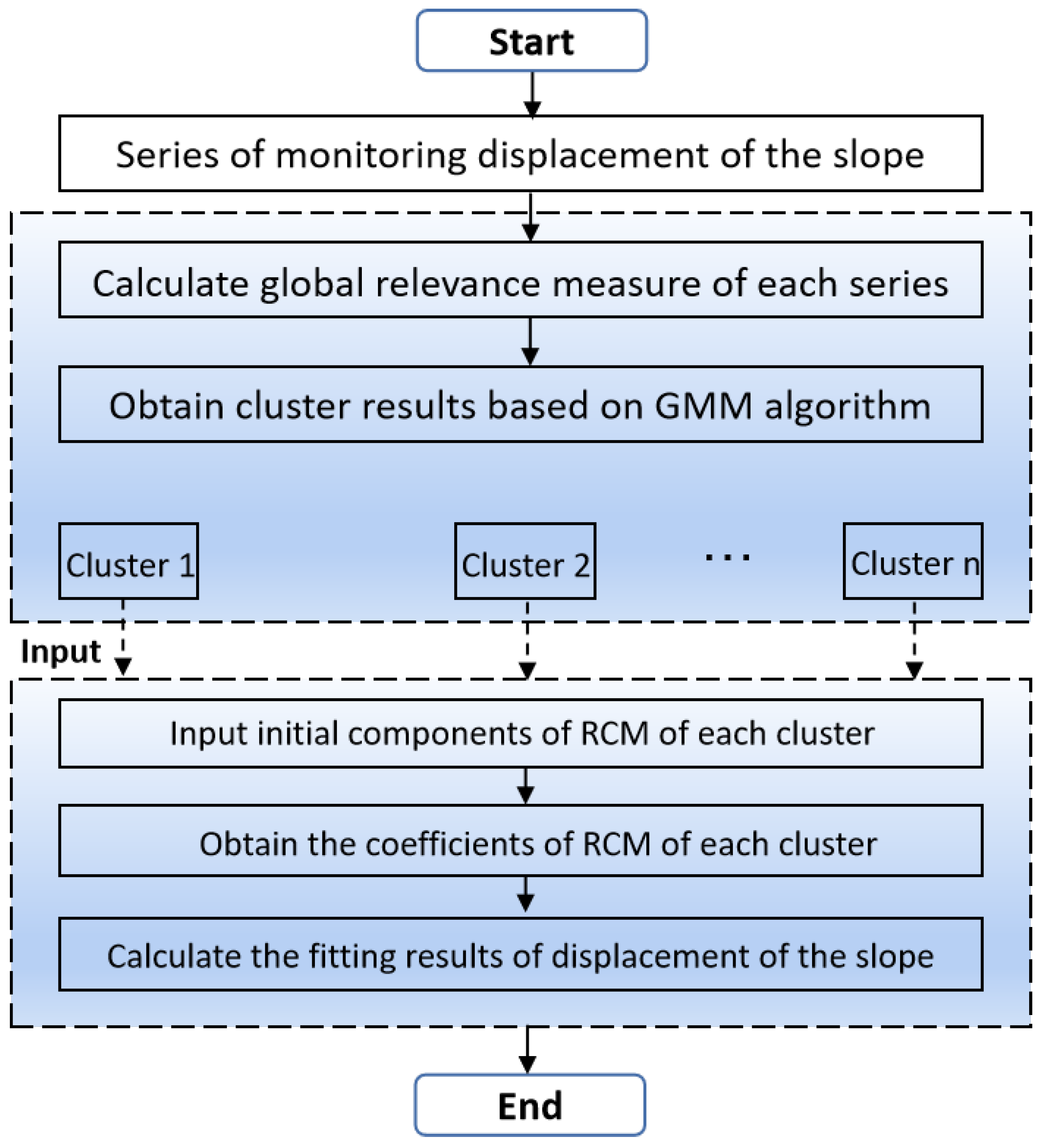
2. Model Development
2.1. Data Clustering Based on Gaussian Mixture Model
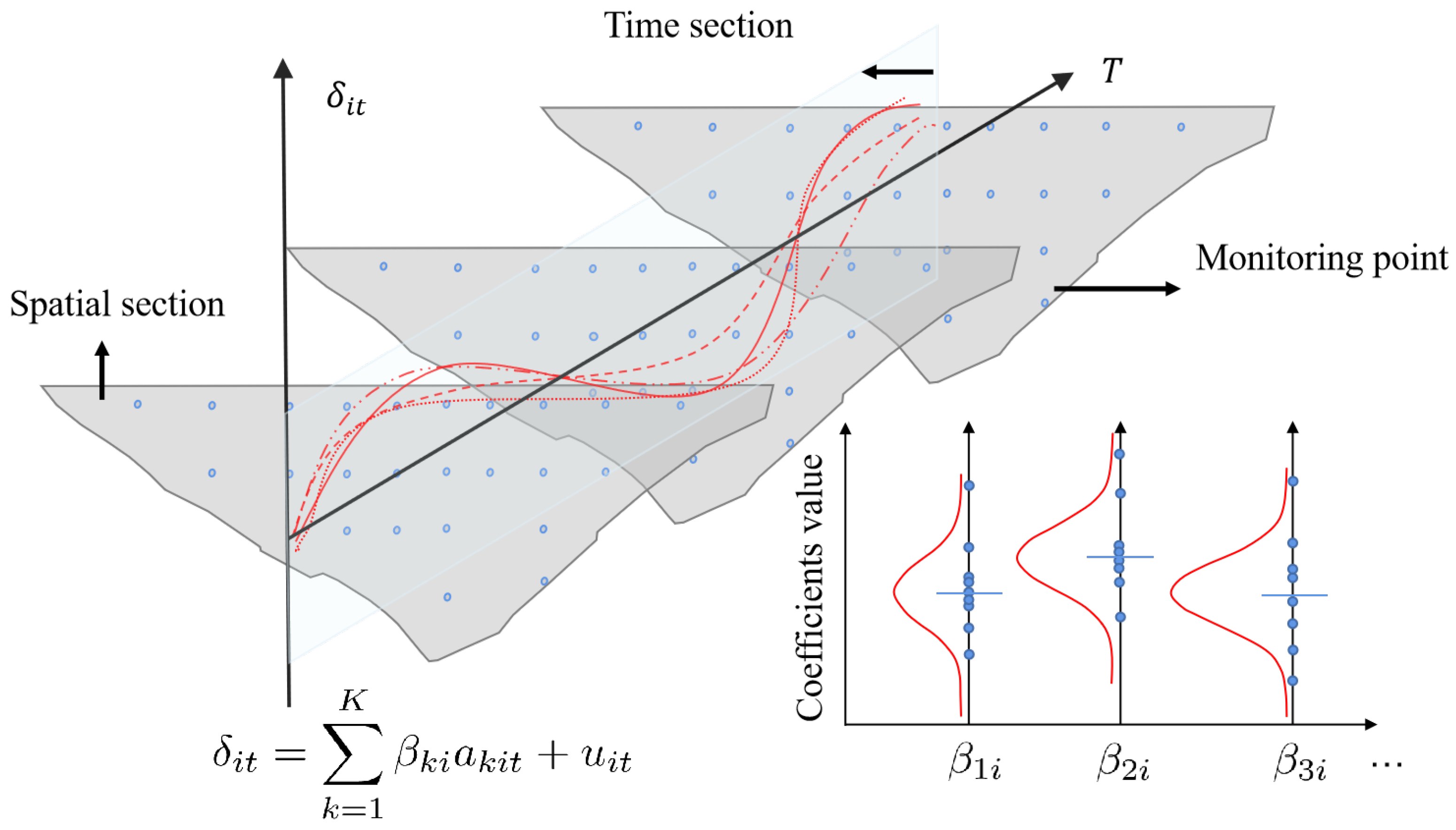
2.2. Random Coefficient Model
3. Study Area and Dataset
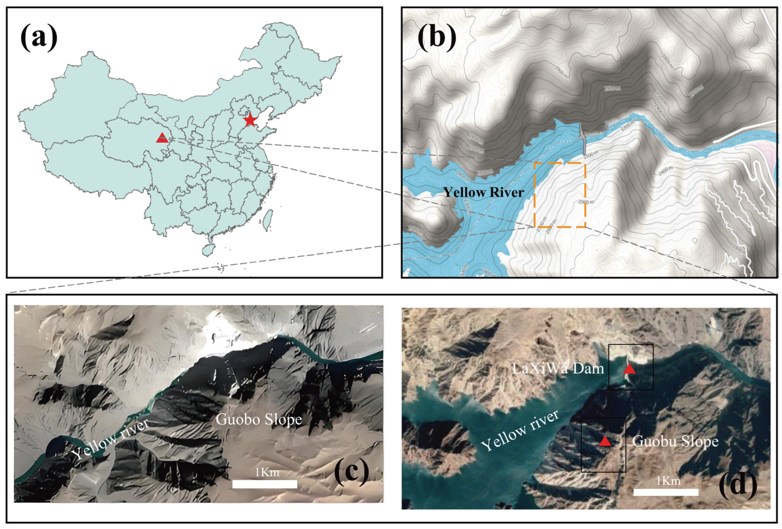
3.1. Study Area
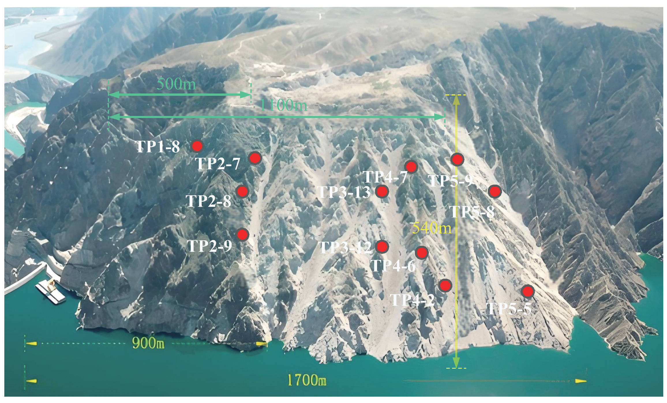
3.2. Dataset
4. Results and Discussions
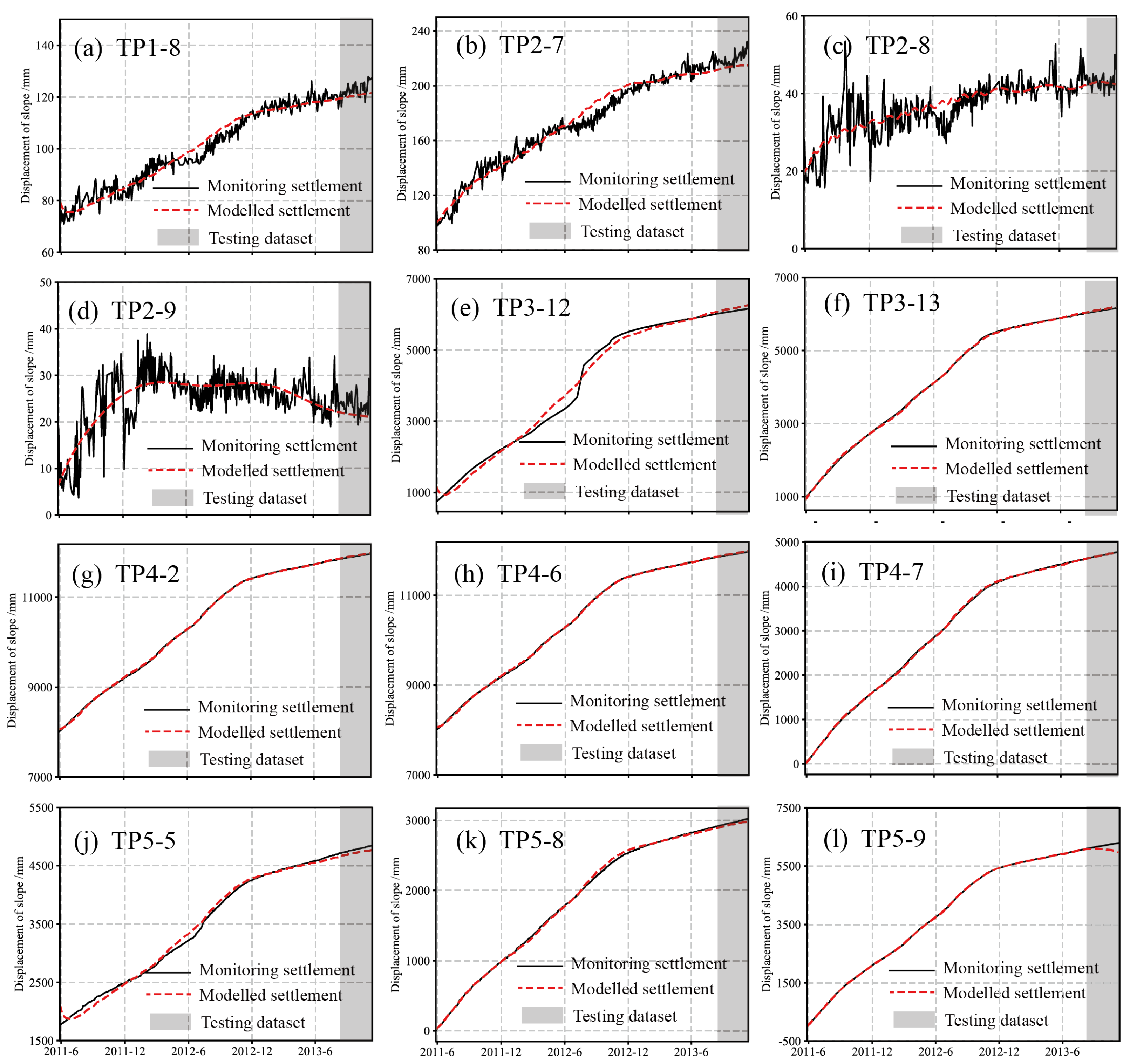
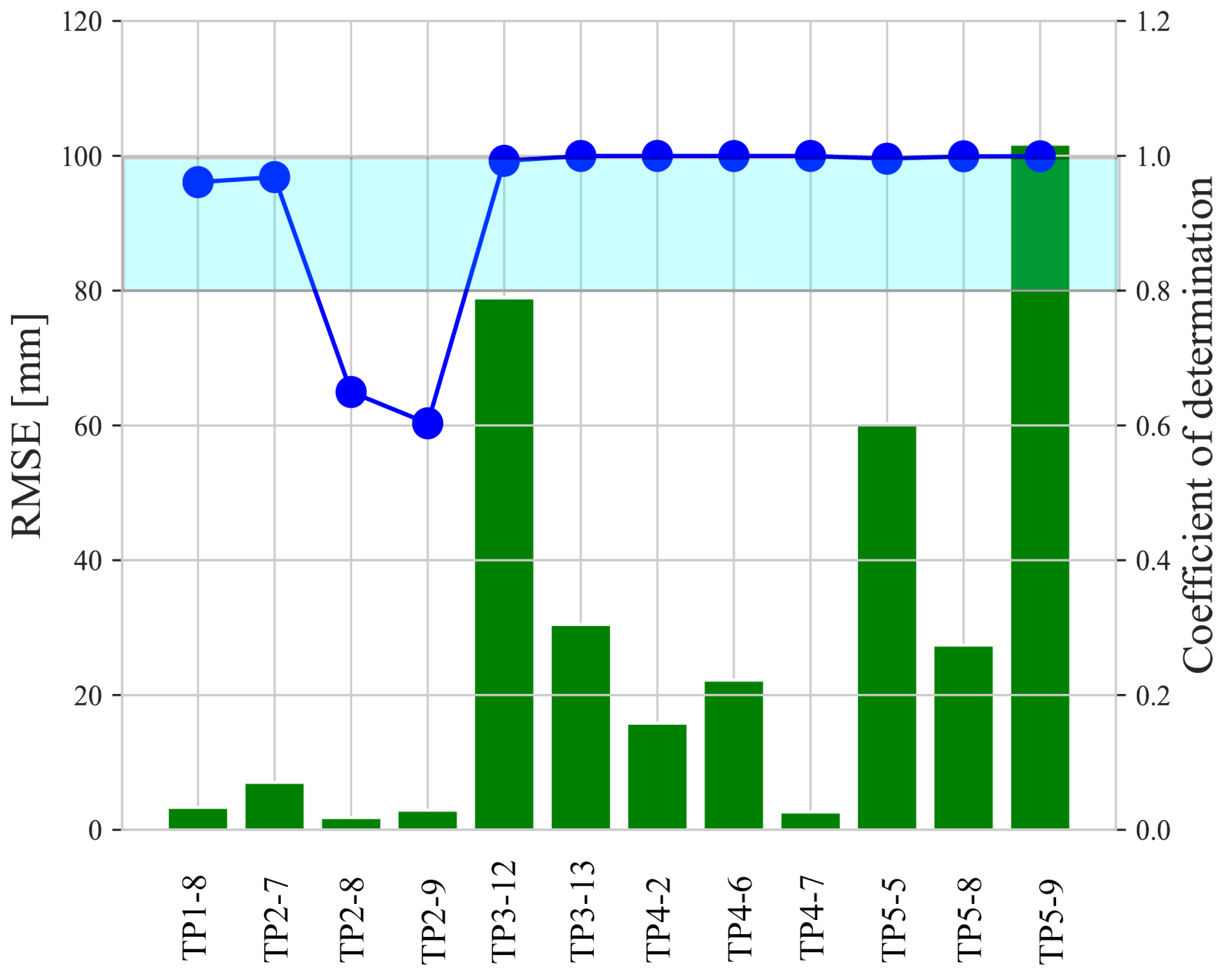
4.1. Prediction Using RCM-GMM Model
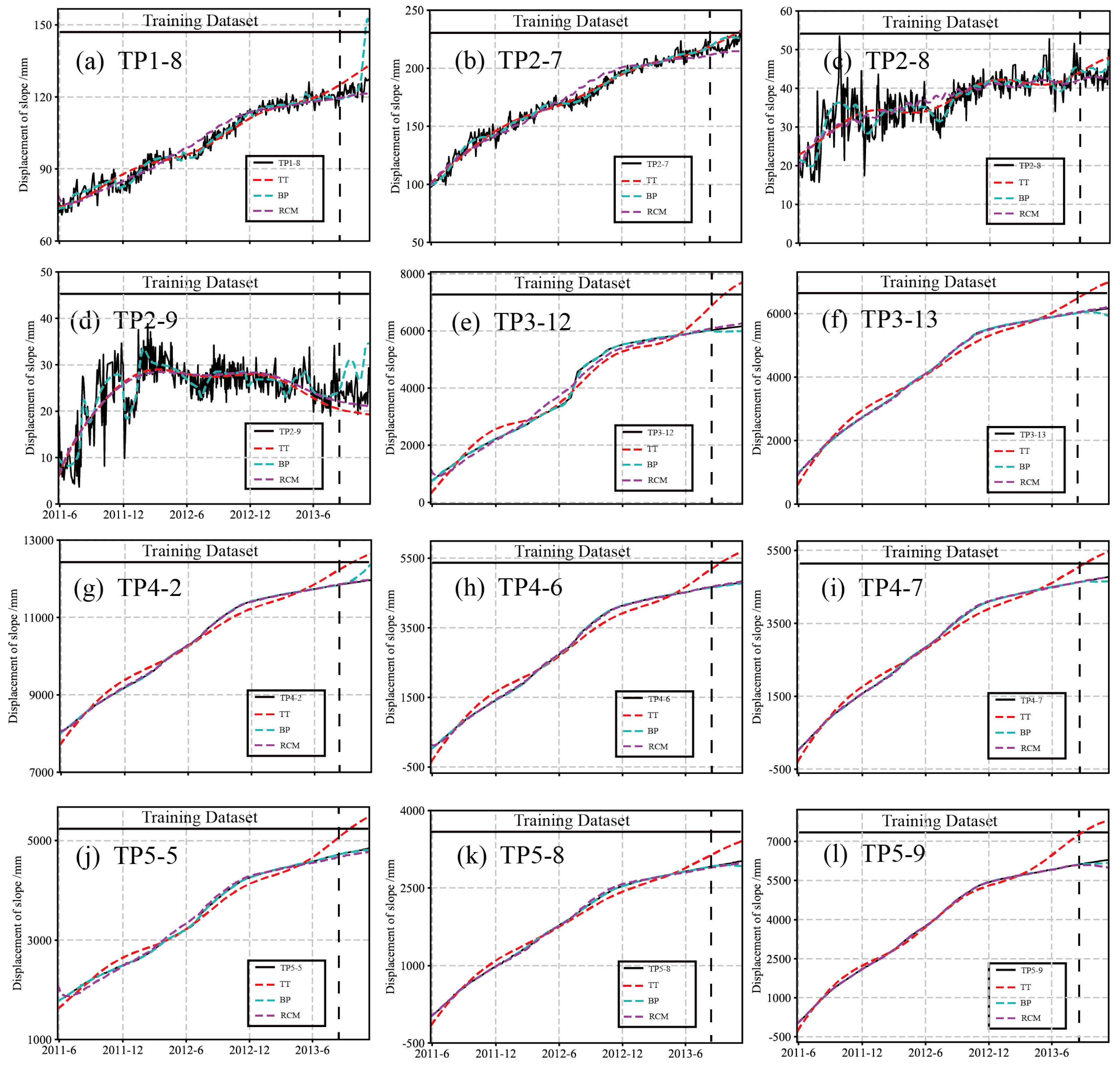
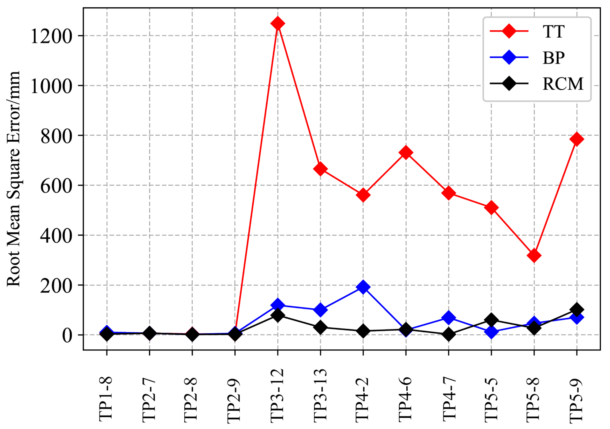
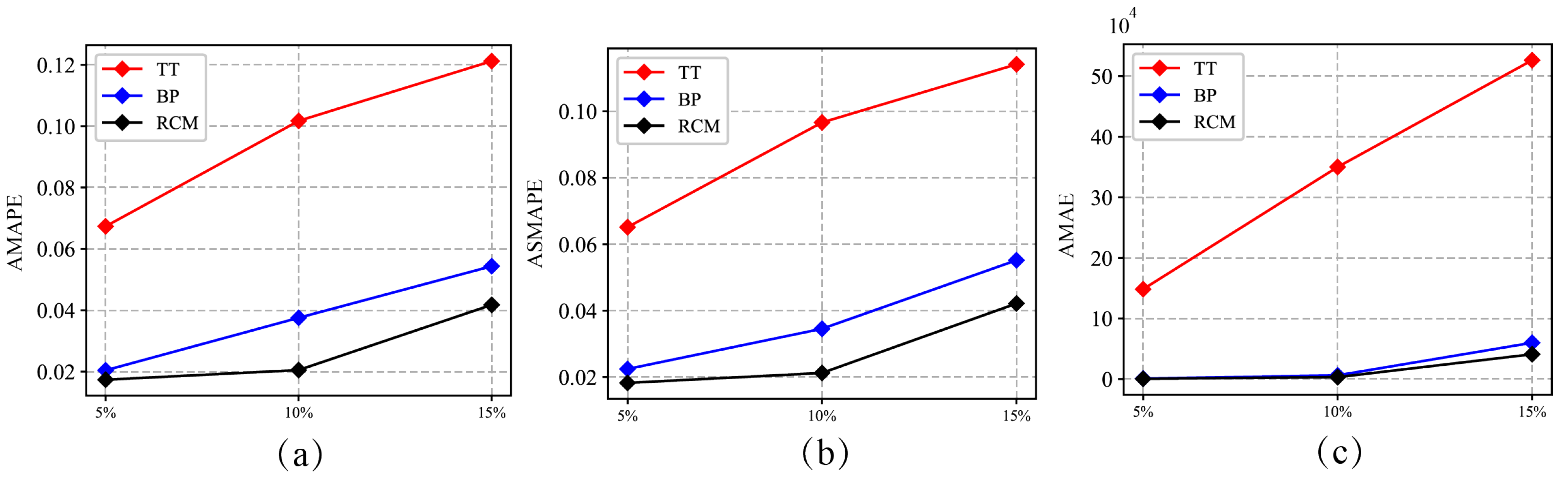
4.2. Comparison of the Prediction Performance of RCM with BP and TT
5. Conclusions
Author Contributions
Funding
Institutional Review Board Statement
Informed Consent Statement
Data Availability Statement
Conflicts of Interest
References
- Meng, Z. Experimental study on impulse waves generated by a viscoplastic material at laboratory scale. Landslides 2018, 15, 1173–1182. [Google Scholar] [CrossRef]
- Wasowski, J.; Bovenga, F. Investigating landslides and unstable slopes with satellite Multi Temporal Interferometry: Current issues and future perspectives. Eng. Geol. 2014, 174, 103–138. [Google Scholar] [CrossRef]
- Liu, X.; Liu, Y.; Yang, Z.; Li, X. A novel dimension reduction-based metamodel approach for efficient slope reliability analysis considering soil spatial variability. Comput. Geotech. 2024, 172, 106423. [Google Scholar] [CrossRef]
- Raucoules, D.; De Michele, M.; Malet, J.P.; Ulrich, P. Time-variable 3D ground displacements from high-resolution synthetic aperture radar (SAR). Application to La Valette landslide (South French Alps). Remote Sens. Environ. 2013, 139, 198–204. [Google Scholar] [CrossRef]
- Schuster, R. Reservoir-induced landslides. Bull. Eng. Geol. Environ. 1979, 20, 8. [Google Scholar] [CrossRef]
- Chen, H.; Huang, S.; Xu, Y.P.; Teegavarapu, R.S.; Guo, Y.; Nie, H.; Xie, H. Using baseflow ensembles for hydrologic hysteresis characterization in humid basins of Southeastern China. Water Resour. Res. 2024, 60, e2023WR036195. [Google Scholar] [CrossRef]
- Perissin, D.; Prati, C.; Rocca, F.; Wang, T. PSInSAR analysis over the Three Gorges Dam and urban areas in China. In Proceedings of the 2009 Joint Urban Remote Sensing Event, Shanghai, China, 20–22 May 2009; IEEE: Piscataway, NJ, USA, 2009; pp. 1–5. [Google Scholar]
- Shi, X.; Zhang, L.; Tang, M.; Li, M.; Liao, M. Investigating a reservoir bank slope displacement history with multi-frequency satellite SAR data. Landslides 2017, 14, 1961–1973. [Google Scholar] [CrossRef]
- Shi, X.; Jiang, H.; Zhang, L.; Liao, M. Landslide displacement monitoring with split-bandwidth interferometry: A case study of the shuping landslide in the three gorges area. Remote Sens. 2017, 9, 937. [Google Scholar] [CrossRef]
- Tang, H.; Wasowski, J.; Juang, C.H. Geohazards in the three Gorges Reservoir Area, China–Lessons learned from decades of research. Eng. Geol. 2019, 261, 105267. [Google Scholar] [CrossRef]
- Zhou, C.; Cao, Y.; Yin, K.; Wang, Y.; Shi, X.; Catani, F.; Ahmed, B. Landslide characterization applying sentinel-1 images and InSAR technique: The muyubao landslide in the three Gorges Reservoir Area, China. Remote Sens. 2020, 12, 3385. [Google Scholar] [CrossRef]
- Meng, Z.; Ancey, C. The effects of slide cohesion on impulse-wave formation. Exp. Fluids 2019, 60, 151. [Google Scholar] [CrossRef]
- Mohammed, F.; Fritz, H.M. Physical modeling of tsunamis generated by three-dimensional deformable granular landslides. J. Geophys. Res. Ocean. 2012, 117, C11015. [Google Scholar] [CrossRef]
- Meng, Z.; Hu, J.; Zhang, J.; Zhang, L.; Yuan, Z. The Momentum Transfer Mechanism of a Landslide Intruding a Body of Water. Sustainability 2023, 15, 13940. [Google Scholar] [CrossRef]
- Ciabatti, M. La Dinamica Della Frana del Vajont; Museo geologico Giovanni Capellini: Bologna, Italy, 1964. [Google Scholar]
- Genevois, R.; Ghirotti, M. The 1963 vaiont landslide. G. Geol. Appl. 2005, 1, 41–52. [Google Scholar]
- Gylfadóttir, S.S.; Kim, J.; Helgason, J.K.; Brynjólfsson, S.; Höskuldsson, Á.; Jóhannesson, T.; Harbitz, C.B.; Løvholt, F. The 2014 L ake A skja rockslide-induced tsunami: Optimization of numerical tsunami model using observed data. J. Geophys. Res. Ocean. 2017, 122, 4110–4122. [Google Scholar] [CrossRef]
- Gauthier, D.; Anderson, S.A.; Fritz, H.M.; Giachetti, T. Karrat Fjord (Greenland) tsunamigenic landslide of 17 June 2017: Initial 3D observations. Landslides 2018, 15, 327–332. [Google Scholar] [CrossRef]
- Pariseau, W.G.; Puri, S.; Schmelter, S.C. A new model for effects of impersistent joint sets on rock slope stability. Int. J. Rock Mech. Min. Sci. 2008, 45, 122–131. [Google Scholar] [CrossRef]
- Griffiths, D.; Marquez, R. Three-dimensional slope stability analysis by elasto-plastic finite elements. Geotechnique 2007, 57, 537–546. [Google Scholar] [CrossRef]
- Bui, H.H.; Fukagawa, R.; Sako, K.; Wells, J.C. Slope stability analysis and discontinuous slope failure simulation by elasto-plastic smoothed particle hydrodynamics (SPH). Géotechnique 2011, 61, 565–574. [Google Scholar] [CrossRef]
- Cundall, P.; Damjanac, B. A comprehensive 3D model for rock slopes based on micromechanics. In Proceedings of the Slope Stability 2009, Santiago, Chile, 9–11 November 2009. [Google Scholar]
- Gurocak, Z.; Alemdag, S.; Zaman, M.M. Rock slope stability and excavatability assessment of rocks at the Kapikaya dam site, Turkey. Eng. Geol. 2008, 96, 17–27. [Google Scholar] [CrossRef]
- Qi, S.; Wu, F.; Yan, F.; Lan, H. Mechanism of deep cracks in the left bank slope of Jinping first stage hydropower station. Eng. Geol. 2004, 73, 129–144. [Google Scholar] [CrossRef]
- Esposito, C.; Martino, S.; Mugnozza, G.S. Mountain slope deformations along thrust fronts in jointed limestone: An equivalent continuum modelling approach. Geomorphology 2007, 90, 55–72. [Google Scholar] [CrossRef]
- Guallini, L.; Brozzetti, F.; Marinangeli, L. Large-scale deformational systems in the South Polar Layered Deposits (Promethei Lingula, Mars): “soft-sediment” and deep-seated gravitational slope deformations mechanisms. Icarus 2012, 220, 821–843. [Google Scholar] [CrossRef]
- Meng, Z.; Wang, Y.; Zheng, S.; Wang, X.; Liu, D.; Zhang, J.; Shao, Y. Abnormal Monitoring Data Detection Based on Matrix Manipulation and the Cuckoo Search Algorithm. Mathematics 2024, 12, 1345. [Google Scholar] [CrossRef]
- Tang, X.S.; Li, D.Q.; Chen, Y.F.; Zhou, C.B.; Zhang, L.M. Improved knowledge-based clustered partitioning approach and its application to slope reliability analysis. Comput. Geotech. 2012, 45, 34–43. [Google Scholar] [CrossRef]
- Meng, Z.; Hu, Y.; Ancey, C. Using a data driven approach to predict waves generated by gravity driven mass flows. Water. 2020, 12, 600. [Google Scholar] [CrossRef]
- Ren, F.; Wu, X.; Zhang, K.; Niu, R. Application of wavelet analysis and a particle swarm-optimized support vector machine to predict the displacement of the Shuping landslide in the Three Gorges, China. Environ. Earth Sci. 2015, 73, 4791–4804. [Google Scholar] [CrossRef]
- Liu, P.; Li, Z.; Hoey, T.; Kincal, C.; Zhang, J.; Zeng, Q.; Muller, J.P. Using advanced InSAR time series techniques to monitor landslide movements in Badong of the Three Gorges region, China. Int. J. Appl. Earth Obs. Geoinf. 2013, 21, 253–264. [Google Scholar] [CrossRef]
- Sezer, E. A computer program for fractal dimension (FRACEK) with application on type of mass movement characterization. Comput. Geosci. 2010, 36, 391–396. [Google Scholar] [CrossRef]
- Li, X.; Kong, J. Application of GA–SVM method with parameter optimization for landslide development prediction. Nat. Hazards Earth Syst. Sci. 2014, 14, 525–533. [Google Scholar] [CrossRef]
- Yiqing, L.; Hongfu, L. Prediction of landslide displacement using grey and artificial neural network theories. Adv. Sci. Lett. 2012, 11, 511–514. [Google Scholar] [CrossRef]
- Zhou, C.; Yin, K.; Cao, Y.; Ahmed, B. Application of time series analysis and PSO–SVM model in predicting the Bazimen landslide in the Three Gorges Reservoir, China. Eng. Geol. 2016, 204, 108–120. [Google Scholar] [CrossRef]
- Zhang, D.; Wang, G.; Yang, T.; Zhang, M.; Chen, S.; Zhang, F. Satellite remote sensing-based detection of the deformation of a reservoir bank slope in Laxiwa Hydropower Station, China. Landslides 2013, 10, 231–238. [Google Scholar] [CrossRef]
- Lin, P.; Liu, X.; Hu, S.; Li, P. Large deformation analysis of a high steep slope relating to the Laxiwa Reservoir, China. Rock Mech. Rock Eng. 2016, 49, 2253–2276. [Google Scholar] [CrossRef]
- Li, M.; Zhang, L.; Shi, X.; Liao, M.; Yang, M. Monitoring active motion of the Guobu landslide near the Laxiwa Hydropower Station in China by time-series point-like targets offset tracking. Remote Sens. Environ. 2019, 221, 80–93. [Google Scholar] [CrossRef]
- Pang, L.; Li, C.; Liu, D.; Zhang, F.; Chen, B. Response of Guobu Slope Displacement to Rainfall and Reservoir Water Level with Time-Series InSAR and Wavelet Analysis. Appl. Sci. 2023, 13, 5141. [Google Scholar] [CrossRef]
- Semenza, E.; Ghirotti, M. History of the 1963 Vaiont slide: The importance of geological factors. Bull. Eng. Geol. Environ. 2000, 59, 87–97. [Google Scholar] [CrossRef]


| Monitoring Point | Coordinate x (m) | Coordinate y (m) | Coordinate z (m) |
|---|---|---|---|
| TP1-8 | 3053.13 | 6483.37 | 2830.24 |
| TP2-7 | 2896.17 | 6369.15 | 2802.69 |
| TP2-8 | 2978.88 | 6274.93 | 2701.89 |
| TP2-9 | 3088.51 | 6164.12 | 2602.38 |
| TP3-12 | 2845.30 | 5946.82 | 2592.63 |
| TP3-13 | 2720.19 | 6070.24 | 2703.45 |
| TP4-2 | 2705.62 | 5789.85 | 2547.86 |
| TP4-6 | 2693.06 | 5859.02 | 2602.79 |
| TP4-7 | 2542.74 | 6053.20 | 2783.44 |
| TP5-5 | 2442.54 | 5621.43 | 2497.97 |
| TP5-8 | 2458.04 | 5956.94 | 2732.45 |
| TP5-9 | 2515.49 | 6103.51 | 2825.94 |
| Monitoring Point | TT | BP | RCM |
|---|---|---|---|
| TP1-8 | 0.9594 | 0.9452 | 0.9610 |
| TP2-7 | 0.9834 | 0.9875 | 0.9684 |
| TP2-8 | 0.6445 | 0.7926 | 0.6496 |
| TP2-9 | 0.6032 | 0.6866 | 0.6032 |
| TP3-12 | 0.9285 | 0.9994 | 0.9926 |
| TP3-13 | 0.9713 | 0.9996 | 0.9998 |
| TP4-2 | 0.9656 | 0.9976 | 0.9998 |
| TP4-6 | 0.9618 | 0.9998 | 0.9998 |
| TP4-7 | 0.9745 | 0.9998 | 0.9999 |
| TP5-5 | 0.9608 | 0.9999 | 0.9957 |
| TP5-8 | 0.9797 | 0.9997 | 0.9993 |
| TP5-9 | 0.9722 | 0.9999 | 0.9993 |
Disclaimer/Publisher’s Note: The statements, opinions and data contained in all publications are solely those of the individual author(s) and contributor(s) and not of MDPI and/or the editor(s). MDPI and/or the editor(s) disclaim responsibility for any injury to people or property resulting from any ideas, methods, instructions or products referred to in the content. |
© 2024 by the authors. Licensee MDPI, Basel, Switzerland. This article is an open access article distributed under the terms and conditions of the Creative Commons Attribution (CC BY) license (https://creativecommons.org/licenses/by/4.0/).
Share and Cite
Yuan, Z.; Bian, Y.; Liu, W.; Qi, F.; Ma, H.; Zheng, S.; Meng, Z. Predicting the Deformation of a Slope Using a Random Coefficient Panel Data Model. Fractal Fract. 2024, 8, 429. https://doi.org/10.3390/fractalfract8070429
Yuan Z, Bian Y, Liu W, Qi F, Ma H, Zheng S, Meng Z. Predicting the Deformation of a Slope Using a Random Coefficient Panel Data Model. Fractal and Fractional. 2024; 8(7):429. https://doi.org/10.3390/fractalfract8070429
Chicago/Turabian StyleYuan, Zhenxia, Yadong Bian, Weijian Liu, Fuzhou Qi, Haohao Ma, Sen Zheng, and Zhenzhu Meng. 2024. "Predicting the Deformation of a Slope Using a Random Coefficient Panel Data Model" Fractal and Fractional 8, no. 7: 429. https://doi.org/10.3390/fractalfract8070429
APA StyleYuan, Z., Bian, Y., Liu, W., Qi, F., Ma, H., Zheng, S., & Meng, Z. (2024). Predicting the Deformation of a Slope Using a Random Coefficient Panel Data Model. Fractal and Fractional, 8(7), 429. https://doi.org/10.3390/fractalfract8070429