
A Novel Contact Resistance Model for the Spherical–Planar Joint Interface Based on Three Dimensional Fractal Theory


Abstract
:1. Introduction
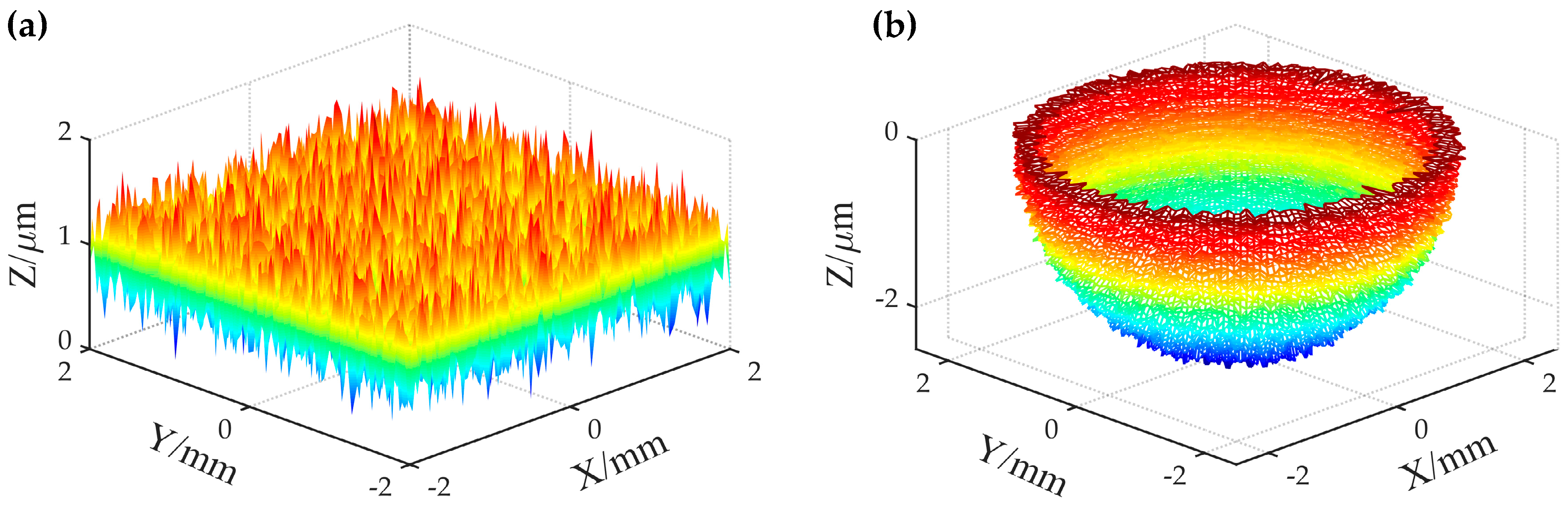
2. Surface Generation Based on Three-Dimensional Fractal Theory
3. Contact Resistance Model for Planar Joint Interface
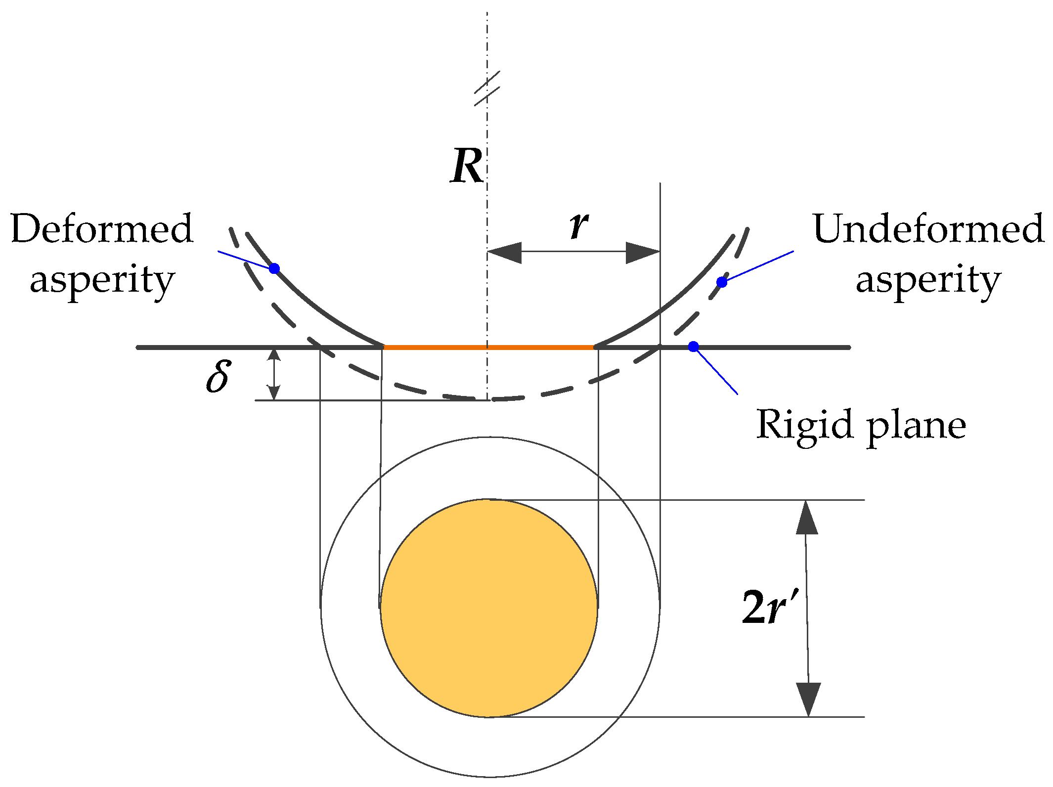
3.1. Contact Mechanics Analysis of Single Asperity
- (1)
- Elastic deformation range
- (2)
- Plastic deformation range
- (3)
- Elastic–plastic deformation range
3.2. Contact Resistance for Planar Joint Interface
4. Contact Resistance Model for Spherical–Planar Joint Interface
4.1. Surface Contact Coefficient
4.2. Contact Resistance for Spherical–Planar Joint Interface
5. Experimental Verification and Simulation Analysis
5.1. Parameters of the Test Samples
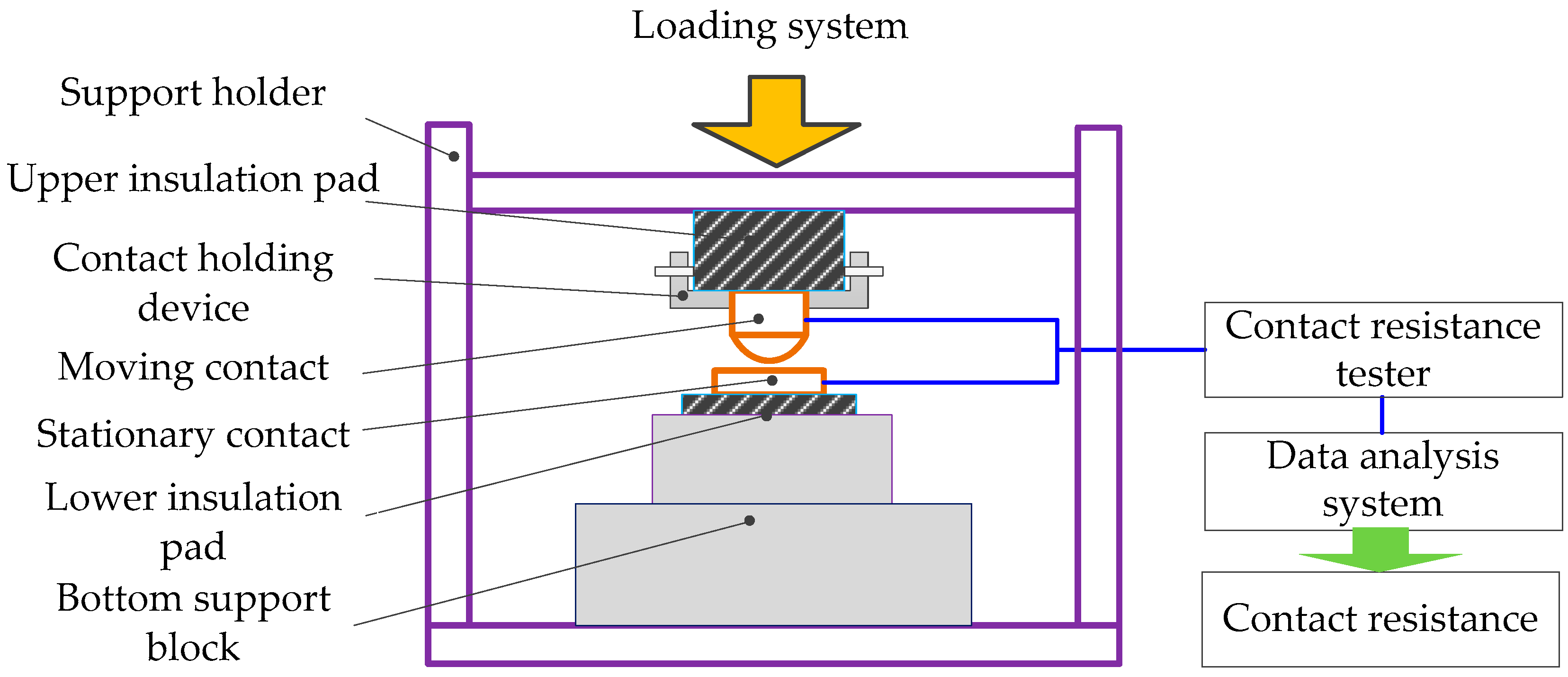
5.2. Experimental Device
5.3. Numerical Simulation and Analysis
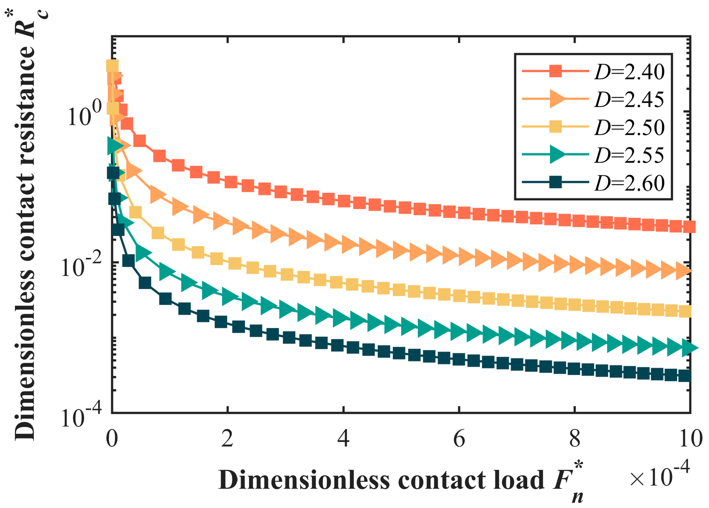
- (1)
- The fractal dimension D
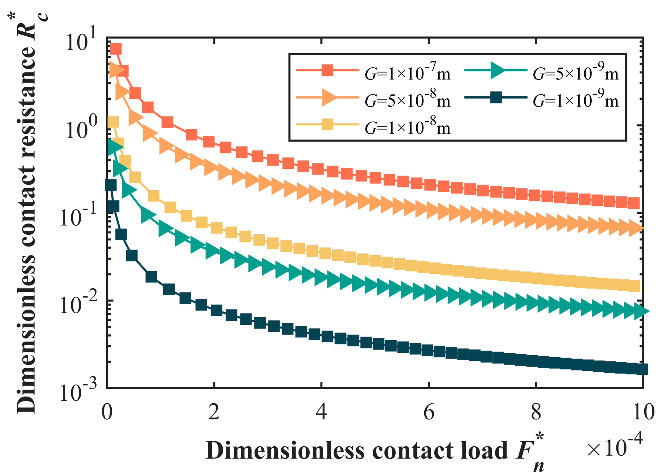
- (2)
- The scale coefficient G
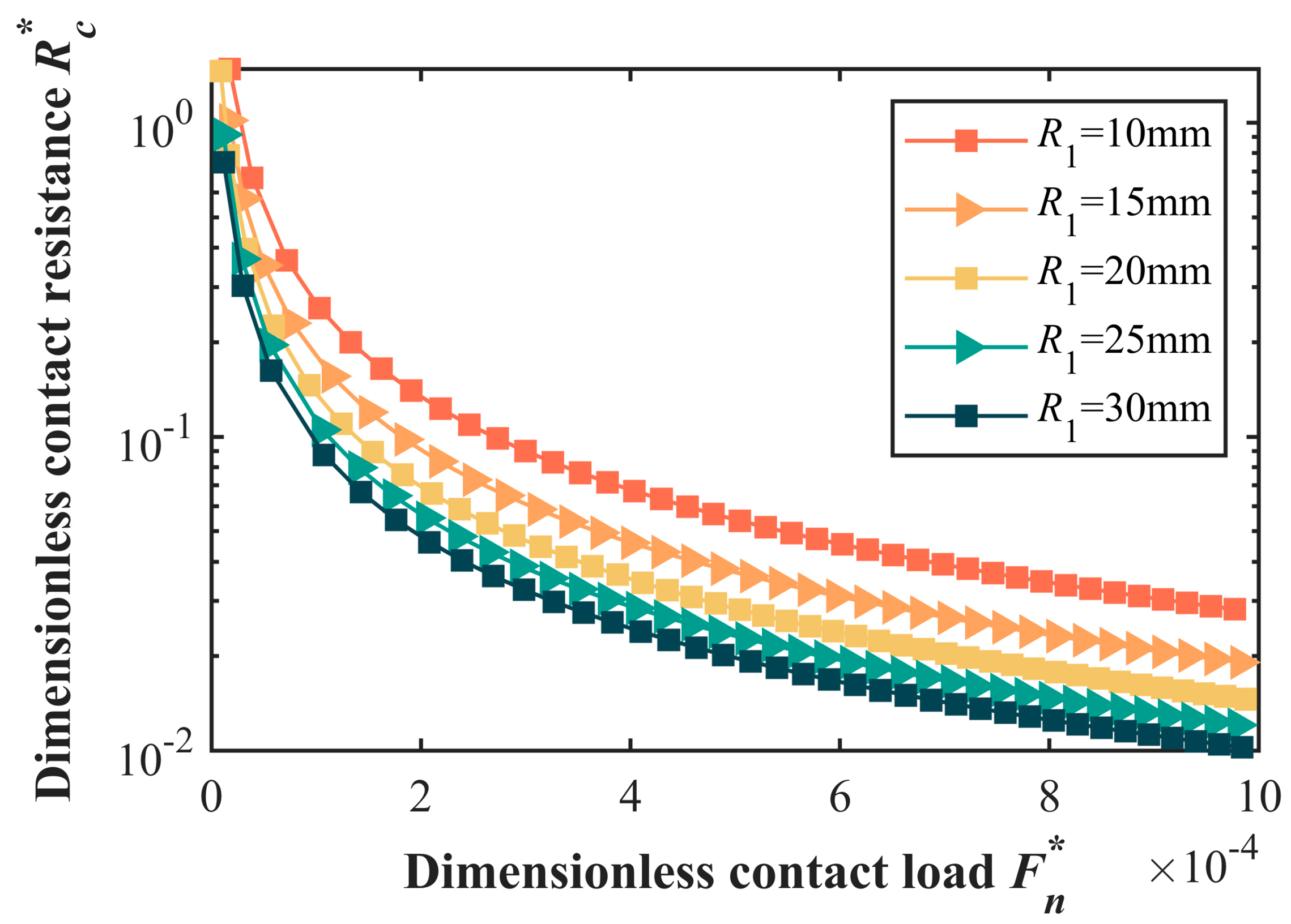
- (3)
- The spherical radius R1
6. Conclusions
- (1)
- A contact resistance model based on three-dimensional fractal theory for the planar joint interface was proposed. In this model, based on three-dimensional fractal theory, the generation of rough surfaces at microscopic scale was achieved. Combining contact mechanics and asperity distribution, a three-dimensional fractal model of contact resistance considering the elastic, elastic–plastic, and plastic deformations in asperities was established.
- (2)
- Combining the contact resistance model for the planar joint interface with the surface contact coefficient, a novel contact resistance model for the spherical–planar joint interface was constructed. By introducing the surface contact coefficient, cross-scale coupling between the macro-geometric sphere and the micro-surface topography was achieved, thereby establishing the contact resistance model for the spherical–planar joint interface.
- (3)
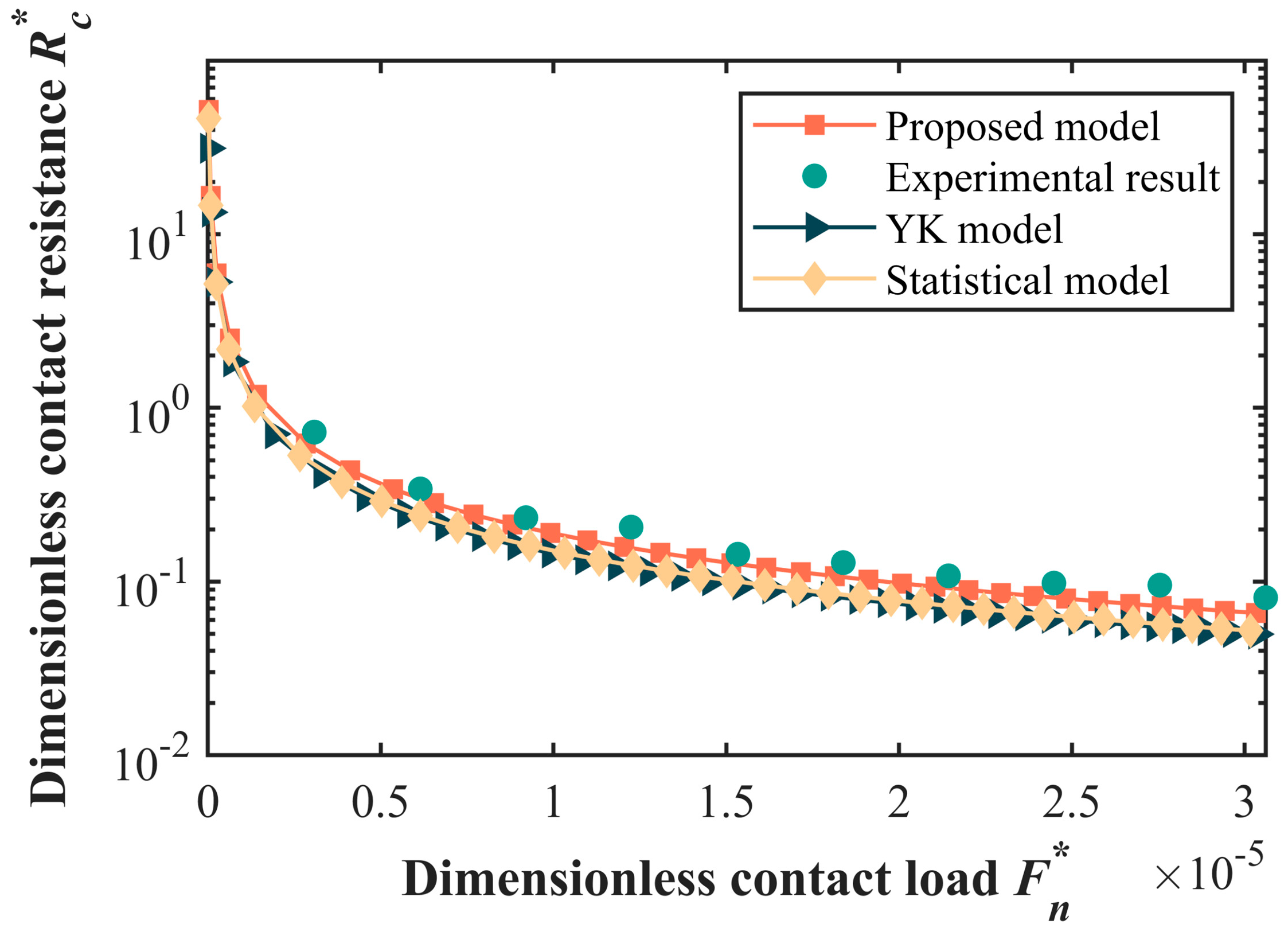
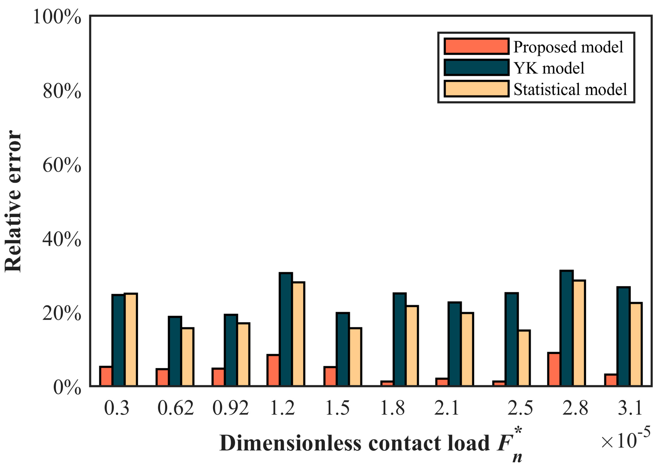
- Experimental verification and simulation analysis was performed on the proposed model. It is worth noting that the model proposed in this paper aligned more closely with the experimental results. Furthermore, the influence mechanism of macro-geometric configuration and micro-surface topography on contact resistance was revealed. The proposed model provides important theoretical and practical value for improving electrical contact performance, optimizing electronic device design, and ensuring the stable operation of power systems.
Supplementary Materials
Author Contributions
Funding
Data Availability Statement
Conflicts of Interest
References
- Dong, Y.Q.; Zhang, P.; Chen, M.J.; Lian, W.L. Numerical study of thermal contact resistance considering spots and gap conduction effects. Tribol. Int. 2024, 193, 109304. [Google Scholar] [CrossRef]
- Cai, Z.B.; Li, C.L.; You, L.; Chen, X.D.; He, L.P.; Cao, Z.Q.; Zhang, Z.N. Prediction of contact resistance of electrical contact wear using different machine learning algorithms. Friction 2024, 12, 1250–1271. [Google Scholar] [CrossRef]
- Sun, X.G.; Xing, W.C. Fractal model of thermal contact conductance of rough surfaces based on elliptical asperity. Ind. Lubr. Tribol. 2023, 75, 424–431. [Google Scholar] [CrossRef]
- Zhang, M.L.; Zuo, X.; Zhou, Y.K. Fractal contact resistance model of wind pitch slip ring considering wear and self-excited vibration. Ind. Lubr. Tribol. 2024, 76, 214–230. [Google Scholar] [CrossRef]
- Holm, R. Electric Contacts: Theory and Applications; Springer: Berlin/Heidelberg, Germany, 1981. [Google Scholar]
- Greenwood, J.A. Constriction resistance and the real area of contact. Br. J. Appl. Phys. 1966, 17, 1621. [Google Scholar] [CrossRef]
- Majumdar, A.; Bhushan, B. Fractal model of elastic-plastic contact between rough surfaces. Tribol. Trans. ASME 1991, 113, 1–11. [Google Scholar] [CrossRef]
- Kogut, L.; Komvopoulos, K. Electrical contact resistance theory for conductive rough surfaces. J. Appl. Phys. 2003, 94, 3153–3162. [Google Scholar] [CrossRef]
- Kogut, L.; Komvopoulos, K. Electrical contact resistance theory for conductive rough surfaces separated by a thin insulating film. J. Appl. Phys. 2004, 95, 576–585. [Google Scholar] [CrossRef]
- Liu, H.; McBride, J. A finite-element-based contact resistance model for rough surfaces: Applied to a bilayered au/mwcnt composite. IEEE Trans. Compon. Packag. Manuf. Technol. 2018, 8, 919–926. [Google Scholar] [CrossRef]
- Li, Y.H.; Shen, F.; Güler, M.A.; Ke, L.L. A rough surface electrical contact model considering the interaction between asperities. Tribol. Int. 2023, 190, 109044. [Google Scholar] [CrossRef]
- Pan, W.J.; Sun, Y.H.; Li, X.M.; Song, H.X.; Guo, J.M. Contact mechanics modeling of fractal surface with complex multi-stage actual loading deformation. Appl. Math. Model. 2024, 128, 58–81. [Google Scholar] [CrossRef]
- Ausloos, M.; Berman, D.H. A multivariate Weierstrass–Mandelbrot function. Proc. R. Soc. A Math. Phys. Eng. Sci. 1985, 400, 331–350. [Google Scholar] [CrossRef]
- Yan, W.; Komvopoulos, K. Contact analysis of elastic-plastic fractal surfaces. J. Appl. Phys. 1998, 84, 3617–3624. [Google Scholar] [CrossRef]
- Jiang, C.Y.; Liang, X.M. An incremental contact model for hyperelastic solids with rough surfaces. Tribol. Lett. 2024, 72, 1. [Google Scholar] [CrossRef]
- Zhang, J.H.; Liu, Y.L.; Yan, K.; Fang, B. A fractal model for predicting thermal contact conductance considering elasto-plastic deformation and base thermal resistances. J. Mech. Sci. Technol. 2019, 33, 475–484. [Google Scholar] [CrossRef]
- Zhang, C.G.; Yu, B.C.; Li, Y.J.; Yang, Q.X. Simplified calculation model for contact resistance based on fractal rough surfaces method. Appl. Sci. 2023, 13, 3648. [Google Scholar] [CrossRef]
- Shen, F.; Li, Y.H.; Ke, L.L. A novel fractal contact model based on size distribution law. Int. J. Mech. Sci. 2023, 249, 108255. [Google Scholar] [CrossRef]
- Liu, Y.; Meng, Q.; Yan, X.; Zhao, S.; Han, J. Research on the solution method for thermal contact conductance between circular-arc contact surfaces based on fractal theory. Int. J. Heat Mass Transf. 2019, 145, 118740. [Google Scholar] [CrossRef]
- Yalpanian, A.; Guilbault, R. A fast correction for half-space theory applied to contact modeling of bodies with curved free surfaces. Tribol. Int. 2020, 147, 106292. [Google Scholar] [CrossRef]
- Li, L.; Etsion, I.; Talke, F.E. Contact area and static friction of rough surfaces with high plasticity index. J. Tribol. 2010, 132, 031401. [Google Scholar] [CrossRef]
- Wang, L.; Xiang, Y. Elastic-plastic contact analysis of a deformable sphere and a rigid flat with friction effect. In Proceedings of the 2nd International Conference on Intelligent Materials and Mechanical Engineering (MEE2012), Yichang, China, 22–23 December 2012; pp. 151–156. [Google Scholar]
- Megalingam, A.; Mayuram, M.M. A comprehensive elastic-plastic single-asperity contact model. Tribol. Trans. 2014, 57, 324–335. [Google Scholar] [CrossRef]
- Zhao, B.; Zhang, S.; Wang, Q.F.; Zhang, Q.; Wang, P. Loading and unloading of a power-law hardening spherical contact under stick contact condition. Int. J. Mech. Sci. 2015, 94–95, 20–26. [Google Scholar] [CrossRef]
- Song, W.P.; Li, L.Q.; Ovcharenko, A.; Talke, F.E. Thermo-mechanical contact between a rigid sphere and an elastic-plastic sphere. Tribol. Int. 2016, 95, 132–138. [Google Scholar] [CrossRef]
- Zhao, B.; Xu, H.Z.; Lu, X.Q.; Ma, X.; Shi, X.J.; Dong, Q.B. Contact behaviors of a power-law hardening elastic-plastic asperity with soft coating flattened by a rigid flat. Int. J. Mech. Sci. 2019, 152, 400–410. [Google Scholar] [CrossRef]
- Chen, W.Z.; Yang, Z.J.; Ding, Z.A. Identifying and evaluating spindle tool-tip dynamic response under different workloads. Mech. Syst. Signal Process. 2023, 185, 109728. [Google Scholar] [CrossRef]
- Zhang, W.Y.; Chen, J.; Wang, C.L.; Liu, D.; Zhu, L.B. Research on Elastic-Plastic Contact Behavior of Hemisphere Flattened by a Rigid Flat. Materials 2022, 15, 4527. [Google Scholar] [CrossRef] [PubMed]
- Zwicker, M.F.R.; Spangenberg, J.; Bay, N.; Martins, P.A.F.; Nielsen, C.V. The influence of strain hardening and surface flank angles on asperity flattening under subsurface deformation at low normal pressures. Tribol. Int. 2022, 167, 107416. [Google Scholar] [CrossRef]
- Kono, D.; Jorobata, Y.; Isobe, H. Holistic multi-scale model of contact stiffness considering subsurface deformation. CIRP Ann.-Manuf. Technol. 2021, 70, 447–450. [Google Scholar] [CrossRef]
- Yu, X.; Sun, Y.Y.; Zhao, D.; Wu, S.J. A revised contact stiffness model of rough curved surfaces based on the length scale. Tribol. Int. 2021, 164, 107206. [Google Scholar] [CrossRef]
- Lu, J.; Xin, Y.; Lochner, E.; Radcliff, K.; Levitan, J. Contact resistivity due to oxide layers between two REBCO tapes. Supercond. Sci. Technol. 2020, 33, 045001. [Google Scholar] [CrossRef]
- Ta, W.R.; Qiu, S.M.; Wang, Y.L.; Yuan, J.Y.; Gao, Y.W.; Zhou, Y.H. Volumetric contact theory to electrical contact between random rough surfaces. Tribol. Int. 2021, 160, 107007. [Google Scholar] [CrossRef]
- Lu, J.; Levitan, J.; McRae, D.; Walsh, R. Contact resistance between two REBCO tapes: The effects of cyclic loading and surface coating. Supercond. Sci. Technol. 2018, 31, 085006. [Google Scholar] [CrossRef]
- Chen, Q.; Xu, F.; Liu, P.; Fan, H. Research on fractal model of normal contact stiffness between two spheroidal joint surfaces considering friction factor. Tribol. Int. 2016, 97, 253–264. [Google Scholar] [CrossRef]
- Fan, X.; Qi, C.; Yunbo, M.; Zhen, A. Research on fractal contact model for contact carrying capacity of two cylinders’ surfaces considering lubrication factors. J. Hefei Univ. Technol. 2017, 40, 169–174. [Google Scholar] [CrossRef]
- Liu, Y.; An, Q.; Huang, M.; Shang, D.; Bai, L. A novel modeling method of micro-topography for grinding surface based on ubiquitiform theory. Fractal Fract. 2022, 6, 341. [Google Scholar] [CrossRef]
- Wang, W.; An, Q.; Suo, S.; Meng, G.; Yu, Y.; Bai, Y. A novel three-dimensional fractal model for the normal contact stiffness of mechanical interface based on axisymmetric cosinusoidal asperity. Fractal Fract. 2023, 7, 279. [Google Scholar] [CrossRef]
- Freiberg, U.; Kohl, S. Box dimension of fractal attractors and their numerical computation. Commun. Nonlinear Sci. Numer. Simul. 2021, 95, 105615. [Google Scholar] [CrossRef]
- Etsion, I.; Levinson, O.; Halperin, G.C.; Varenberg, M. Experimental Investigation of the Elastic-Plastic Contact Area and Static Friction of a Sphere on Flat. J. Tribol.-Trans. ASME 2005, 127, 47–50. [Google Scholar] [CrossRef]


| Material Parameter | Elastic Modulus | Yield Strength | Poisson’s Ratio | Friction Coefficient | Resistivity |
|---|---|---|---|---|---|
| Value | 115 GPa | 220 Mpa | 0.34 | 0.19 | 1.78 × 10⁻⁸ Ω·m |
Disclaimer/Publisher’s Note: The statements, opinions and data contained in all publications are solely those of the individual author(s) and contributor(s) and not of MDPI and/or the editor(s). MDPI and/or the editor(s) disclaim responsibility for any injury to people or property resulting from any ideas, methods, instructions or products referred to in the content. |
© 2024 by the authors. Licensee MDPI, Basel, Switzerland. This article is an open access article distributed under the terms and conditions of the Creative Commons Attribution (CC BY) license (https://creativecommons.org/licenses/by/4.0/).
Share and Cite
An, Q.; Wang, W.; Huang, M.; Suo, S.; Liu, Y.; Wang, S. A Novel Contact Resistance Model for the Spherical–Planar Joint Interface Based on Three Dimensional Fractal Theory. Fractal Fract. 2024, 8, 503. https://doi.org/10.3390/fractalfract8090503
An Q, Wang W, Huang M, Suo S, Liu Y, Wang S. A Novel Contact Resistance Model for the Spherical–Planar Joint Interface Based on Three Dimensional Fractal Theory. Fractal and Fractional. 2024; 8(9):503. https://doi.org/10.3390/fractalfract8090503
Chicago/Turabian StyleAn, Qi, Weikun Wang, Min Huang, Shuangfu Suo, Yue Liu, and Shuai Wang. 2024. "A Novel Contact Resistance Model for the Spherical–Planar Joint Interface Based on Three Dimensional Fractal Theory" Fractal and Fractional 8, no. 9: 503. https://doi.org/10.3390/fractalfract8090503