Abstract
This article investigates the dynamic behaviors of delayed fractional-order memristive fuzzy cellular neural networks via the Lyapunov method. To address the delay terms of fractional-order systems, a novel lemma is provided to make the solutions of the systems exponentially stable. Furthermore, two new intermittent-hold controllers are designed to improve the robustness of the system and reduce the cost of the controller. One intermittent-hold controller is based on the feedback control strategy, while the other one integrates an adaptive control strategy. Moreover, two crucial theorems are derived from the proposed lemma and controllers, guaranteeing the exponential synchronization between drive and response systems. Finally, the superior performance of the controllers in achieving exponential synchronization is demonstrated through simulations.
1. Introduction
A memristor is a kind of basic circuit element introduced by Chua [1]. In 2008, a physical model was proposed, making memristors appropriate for practical applications [2]. Owing to their unique nonlinear characteristics and considerable advantages, memristors have been extensively studied. Inspired by biological concepts, memristors have been applied in neural networks due to their abilities to learn and forget [3]. Therefore, memristors have become a hot topic in various fields, including electrical engineering [4], chaotic circuits [5] and neural networks [6]. Memristor neural networks (MNNs) are complex network systems that integrate the characteristics of memristors and neural networks. The authors of [7] investigated the multistability of MNNs using nonlinear theory and demonstrated the chaotic behavior of memristor-based Hopfield neural networks. Finite time synchronization was proposed through an adaptive control strategy for memristive neural networks in [8]. MNNs can perform chaotic behavior when appropriate parameters are selected, which has attracted significant attention [9,10].
Cellular neural networks (CNNs) were proposed in 1988 in [11], with the connection weights determined according to the characteristics and dynamical behaviors of neurons, reflecting the intrinsic nature of CNNs. CNNs have attracted a lot of attention, as seen in [12,13,14]. Fuzzy cellular neural networks (FCNNs) are a specialized form of CNNs incorporating fuzzy operations that were first proposed in [15]. Fuzzy logic can provide effective features of dynamic behavior, such as increased robustness and stability. The uncertainties in the FCNNs make them well-suited to address nonlinear filtering problems. Furthermore, ref. [16] demonstrated that FCNNs behave well in image processing and recognition. The authors of [17], investigated the mean square stability of FCNNs with mixed delays. The authors of [18] introduced memristive cellular neural networks (MCNNs) by integrating memristors with cellular neural networks. Compared with CNNs, their improved storage capacity makes MCNNs more popular Furthermore, the authors of [19] investigated MCNNs, with fixed-time synchronization conditions established by using feedback controllers and Lyapunov methods. Additionally, ref. [20] reported the synchronization results of memristive neural networks with the fuzzy cellular neural networks (MFCNNs) through feedback controllers. The combination of memristors with FCNNs can expand the advantages of memory, in addition to exhibiting chaotic characteristics.
Fractional-order calculus originated three hundred years ago, although it was not widely promoted due to the lack of physical meanings. Scientists and engineers began to realize that fractional derivatives and integrals can more accurately describe practical phenomena [21]. For instance, the model of a DC–DC converter is a typical fractional-order (FO) system, and its performance is affected if a traditional integer-order model is adopted [22]. In [23], Stamova and Stamov studied fractional-order neural networks (FNNs) with delays and reaction–diffusion. The concept of FO cellular neural networks was proposed by the authors of [24]. The authors of [25] integrated fuzzy logic into FO cellular neural networks. With the efforts of scholars, FNNs have become increasingly significant, with their dynamic properties, such as stability and synchronization, having received extensive attention. The introduction of FO memristive neural networks (FMNNs) is discussed in [26]. Since then, many efforts have been made in the study of FMNNs. For instance, FO memristive fuzzy cellular neural networks (FMFCNNs), which integrate fuzzy logic with fractional-order MNNs, have been explored, with finite-time stability results reported in [27]. The authors of [28,29] studied FMFCNNs for finite-time synchronization and fixed-time synchronization, respectively. However, the authors of [28] did not employ the Lyapunov method, and the authors of [29] used an integer-order derivative to handle the Lyapunov function. Research on FMFCNNs, particularly concerning exponential synchronization, remains limited. This is one of the motivations of this paper.
Synchronization is a critical dynamic behavior that has been extensively studied. Controller design is a core problem, and there are many effective traditional controllers [30,31,32,33]. Intermittent controllers stand out as an economical option that can reduce control resource loss and is easy to achieve. From the perspective of engineering, the transmitted information may be interrupted by disturbances, which means discontinuous controllers are more suitable for practical applications. The authors of [34,35] investigated the synchronization of neural networks using an intermittent controller. In [36], a novel intermittent-hold controller was proposed that extends traditional intermittent control by incorporating holding time, allowing the system to retain state information when communication is interrupted. This enhancement increases the robustness of the system. Traditional intermittent control strategies set the control input to zero during communication interruptions, which may cause a decreased convergence rate. However, intermittent-hold control strategies can improve this phenomenon, as demonstrated in [37]. Moreover, intermittent-hold control strategies simplify the design of controllers by not updating the control input during communication interruptions, thereby reducing the cost of controllers. But this kind of controller has not been applied in FNNs. For delayed FNNs, achieving exponential synchronization is challenging due to the distinct principles of fractional derivatives compared to integer-order derivatives. To address this, we present an inequality to handle delay terms and study exponential synchronization problems of FMFCNNs.
Moreover, in practical applications, chaotic synchronization can be utilized in secure communications. For example, the authors of [38] considered the synchronization problems of the MNNs and achieved encryption and decryption. Due to the enriched dynamical behaviors and the expanded parameter spaces of FO systems, the neural networks represented by FO calculus have more unpredictable dynamics. These characteristics make secure communication problems based on FO systems more complicated [39]. The study reported in [40] exhibits the robustness of FO systems, implying that such systems can ensure the stability and reliability of secure communication, even in unstable communication environments and under external interference. Inspired by the above discussion, this paper designs an intermittent-hold controller of FO systems and applies the synchronization results to secure communication problems.
The exponential synchronization of the FMFCNNs is achieved in this paper, and a novel intermittent-hold controller is designed. The main contributions are summarized as follows:
- (1)
- In this paper, a novel intermittent-hold controller is designed. The controller can chose control time flexibly with less control loss. Furthermore, adaptive control is integrated with intermittent-hold control to handle more complicated situations such as uncertainties and chaos.
- (2)
- A new inequality is introduced to provide the exponential stability condition for fractional-order (FO) systems, overcoming the challenges in constructing Lyapunov functions for FO systems. Based on this novel inequality, the exponential synchronization of FMFCNNs is achieved.
- (3)
- Some examples are provided to demonstrate the effectiveness of the proposed conditions. The control time and resting time can be chosen as required, and larger delays can be tackled by using the proposed conditions and controller, as shown in simulations.
- (4)
- The conditions can be applied to secure communication problems, as shown in Example 3. The chaotic signal generated by the FO drive system is mixed with the original signal for encryption. The decrypted signal is recovered through synchronized response systems.
The remainder of this paper is structured as follows. Some lemmas, definitions and models used in this paper are described in Section 2. Two types of intermittent-hold controllers are designed and some new lemmas and theorems are provided in Section 3. Three examples of three-dimensional and two-dimensional cases, as well as secure communications, are presented in Section 4. The last part discusses future work and our proposed conclusions.
2. Preliminaries and Models
This section contains a description of FMFCNNs and introduces some lemmas used in this paper.
2.1. Model Description
Consider the following fuzzy cellular FMNNs:
where denotes the initial condition, is the self-feedback coefficient, and and are the memristor’s connective weights. is the time delay, and and are feedback functions. In the fuzzy cellular neural network model, and are elements of fuzzy feedback, is MIN and other is MAX. The MIN of a fuzzy feed-forward neural network is , and MAX is . , ⋀ and ⋁ are bias of the ith neuron and fuzzy AND and OR, respectively. The memristive weights of and are satisfied as follows:
where is a switching jump and , , and represent memristance-related constants.
Regarding (1) as drive systems, the response systems of fuzzy cellular FMNNs can be described as follows:
where the initial condition is , and is the intermittent hold controller. The memristor’s connection weights ( and ) are denoted as follows:
According to Filippov and differential inclusion theories, there exist measurable functions, i.e., , , where represents the minimum of , denotes the maximum of and and stand for and , respectively. Then the FO neural networks (1) can be rewritten as follows:
There exist measurable functions, i.e., , , where represents the minimum of and denotes the maximum of . and stand for and , respectively. The response systems can be described as follows:
The error is denoted as , and the error system of (5) and (6) is expressed as follows:
When the error system is stable under controller , systems (5) and (6) can achieve synchronization. Therefore, the subsequent sections focus on designing controllers and investigating the synchronization problems.
2.2. Preliminaries
In this subsection, some useful assumption and lemmas are presented, along with the definition of a Caputo derivative. The models proposed in this paper are described using the Caputo derivative.
Definition 1
([41]). For -order continuous differentiable functions (), the Caputo fractional-order derivative is defined as follows:
where and is an integer.
Assumption A1.
Activation functions and satisfy the following for all , , :
where and are Lipschitz constants.
Lemma 1
([42]). Based on Assumption 1, for measurable functions (, ), then
where , .
Lemma 2
([16]). For system (5), we have the following:
where and are states of system (5).
Lemma 3
([43]). For a continuous function (), for , there exist constants (ρ and δ) such that
Then, we can obtain
3. Main Results
A novel intermittent-hold controller is designed and the control strategies are given in this section. Feedback control and adaptive control are integrated with intermittent-hold control. Some sufficient conditions for achieving exponential synchronization of FO systems are provided in this part.
3.1. Controller Design
Consider following intermittent controller:
In contrast with traditional intermittent control, the intermittent-hold control strategy remains the last received state information of the system instead of stopping control input. By selecting the appropriate holding interval, drive and response systems can achieve synchronization faster. In addition, the intermittent-hold control strategy is less conservative than traditional intermittent control and can achieve synchronization even with shorter communication intervals [44]. The time intervals are , , and . The controller can be designed as follows:
where the control gains ( and ) need to be designed later. Controller (14) can be designed as an adaptive intermittent-hold controller as follows:
where , , and are constants.
Remark 1.
Controller (14) adopts an intermittent-hold control strategy, allowing for flexible selection of control time and holding time. By using this controller, larger delays can be tackled as shown in Figure 8. Controller (15) is feedback-based, and controller (16) is adaptive-based so that it can handle more complex situations. The design of control gains is addressed subsequently.
Remark 2.
The use of an adaptive controller is an intelligent control strategy. The control law includes an update rule to adjust the control parameters. These parameters are dynamically updated based on errors and state changes between drive and response systems. The design of control parameters and needs to be determined by the conditions outlined in Theorem 2.
3.2. Exponential Synchronization of FMNNs with Fuzzy Cellular Neural Networks
In this subsection, a lemma for a delayed FO system is presented that addresses the exponential stability and synchronization problems. The results for FMFCNNs with two kinds of intermittent-hold control are reported.
Lemma 4.
For following delayed FO system with , is exponentially stable if , and is bounded:
Then, there exist positive constants (b and ) such that
Proof of Lemma 4.
For a positive function (), we have
and, taking the FO integral of (17), we can obtain
Then, taking the Laplace transform of (18), we derive the following equation:
where , . From (19), we have
Then, taking the inverse Laplace transform of (20), we can obtain
According to [45], we have , and . Then, we can obtain
Letting , we have
By utilizing grown-wall inequality we obtain
where and, because of , there exists such that . Therefore, we can obtain
□
Remark 3.
When FO systems satisfy the requirements of Lemma 4, decays exponentially. If is a Lyapunov functional, the results of exponential stability or exponential synchronization can be obtained under Lemma 4.
Theorem 1.
Under the assumption 1, if there exists a positive control gain () such that
and
hold, where and other constants are previously defined system parameters, fuzzy cellular FMNNs (5) and (6) can achieve exponential synchronization with controller (15).
The proof of Theorem 1 is shown in Appendix A.
If controller (15) is changed into an adaptive intermittent-hold controller as (16), a different synchronization result can be obtained.
Theorem 2.
Fuzzy cellular FMNNs (5) and (6) can achieve exponential synchronization with adaptive intermittent-hold controller (16) if there exist control gains (, and ) such that
and assumption 1 holds, where and other constants are previously defined system parameters.
The proof of Theorem 2 is given in Appendix B.
Remark 4.
The gains of controllers are determined by the conditions of theorems. For controller (15), the gains () need to satisfy the conditions of Theorem 1, and are given in (29). For controller (16), the of adaptive laws need to satisfy the conditions of Theorem 2. When inequalities in theorems are satisfied with system parameters and control gains, the drive and response systems can achieve synchronization.
4. Simulation
Example 1.
Consider a three-dimensional FMNN with a fuzzy cellular neural network with the following parameters:
where , , and and the activation functions are .
Other parameters are denoted as follows:
Let and ; then, according to Lemma 2 and the above parameters, we can obtain
We can calculate that , and for and that , , and . The control gains of controller (15) satisfy the conditions of Theorem 1 with the above system parameters. Therefore, the drive and response systems can achieve synchronization.
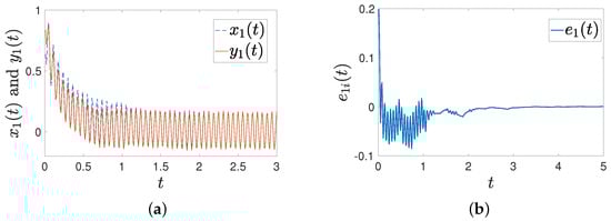
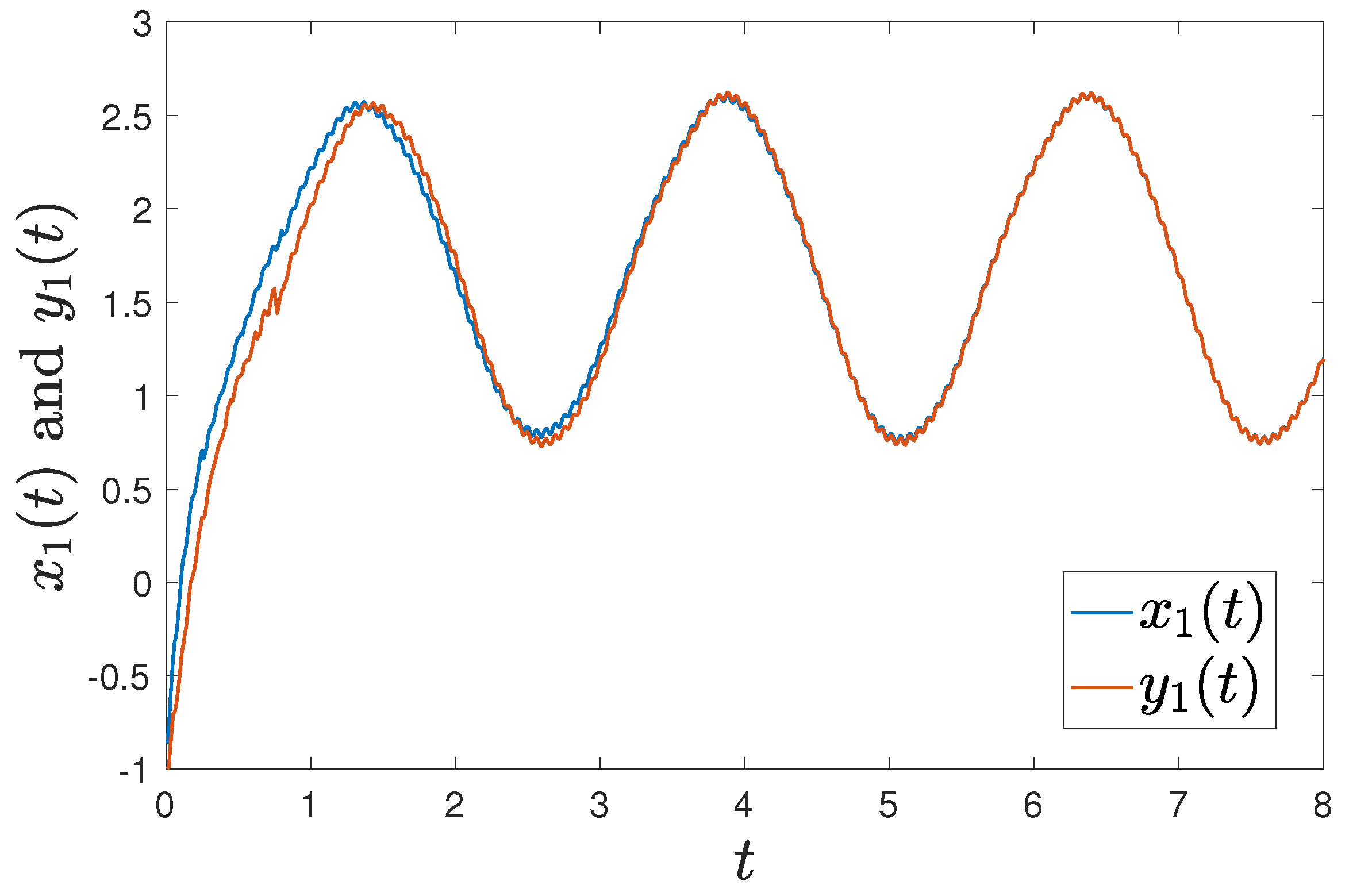
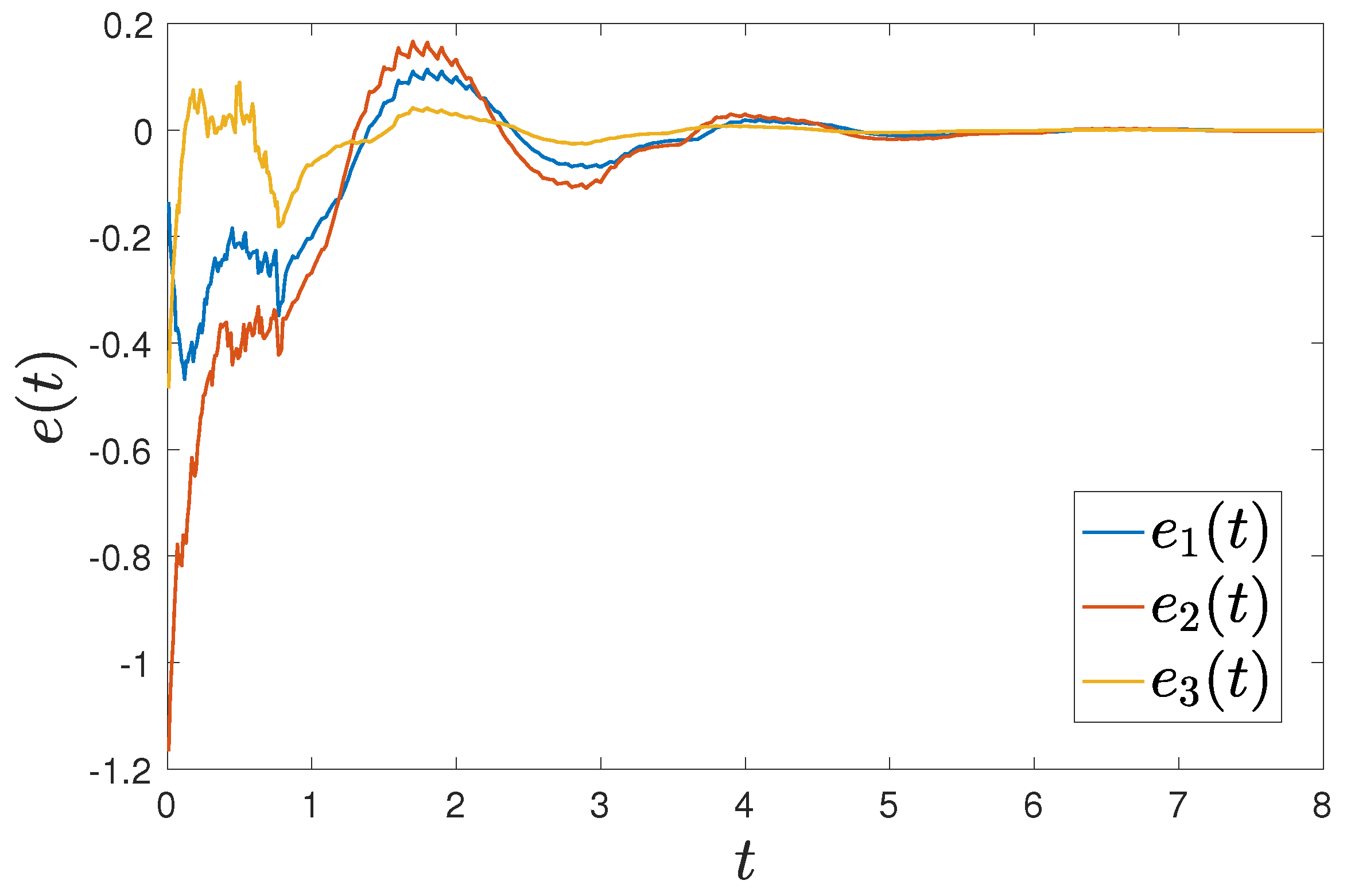
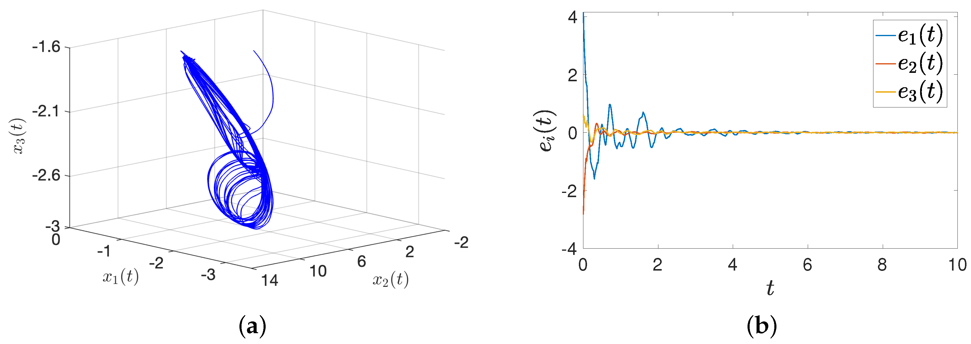
Figure 1 shows that the trajectories of and can achieve synchronization under intermittent-hold controller (15) with initial values of and . Figure 2 shows that the error systems can converge to zero with initial values of and .
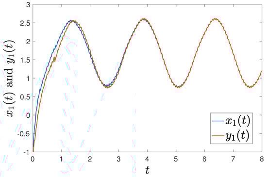
Figure 1.
Trajectories of and under controller (15) with with initial values of and .
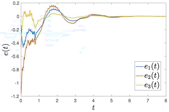
Figure 2.
Trajectories of error between FMNs (5) and (6) under controller (15).
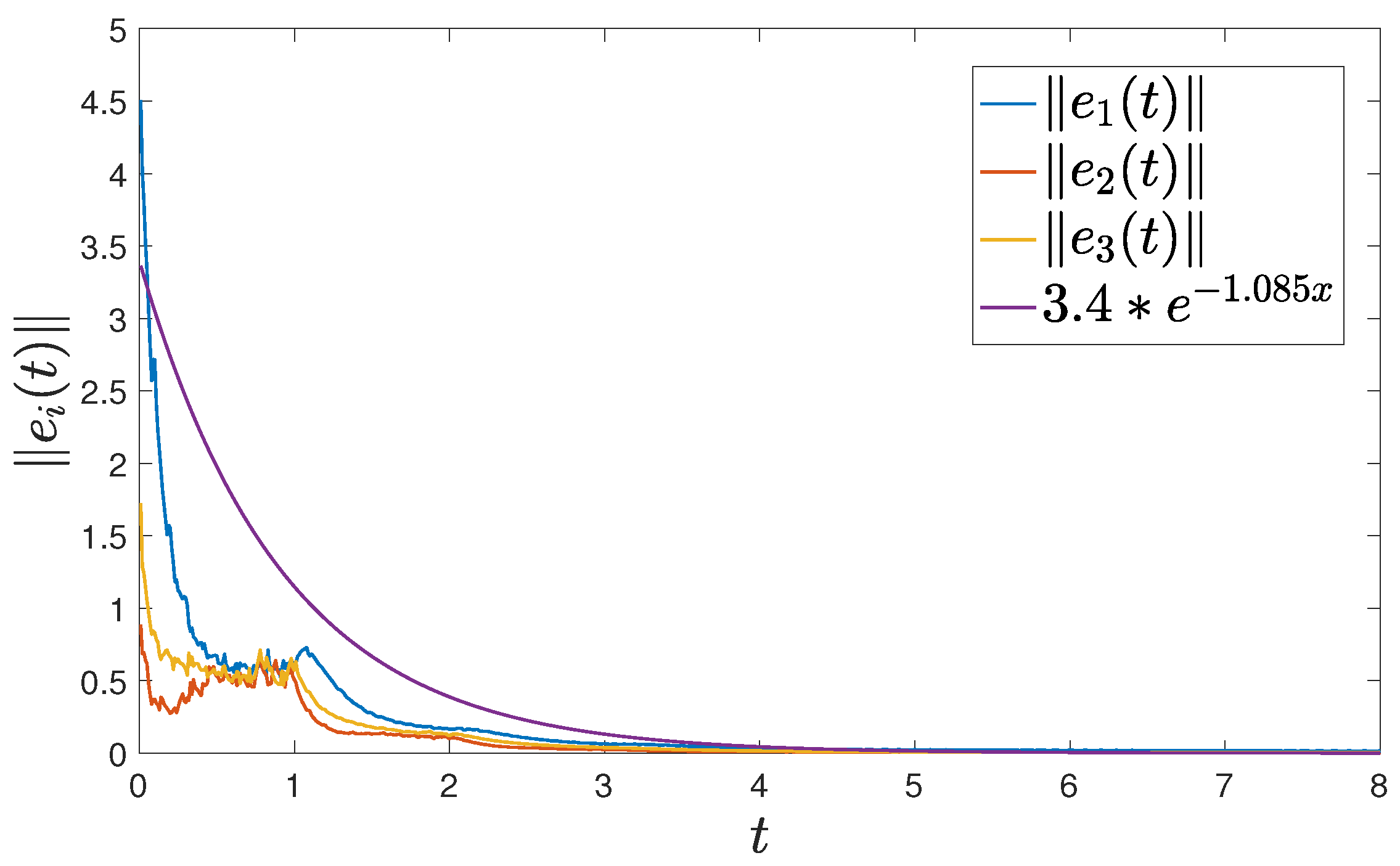
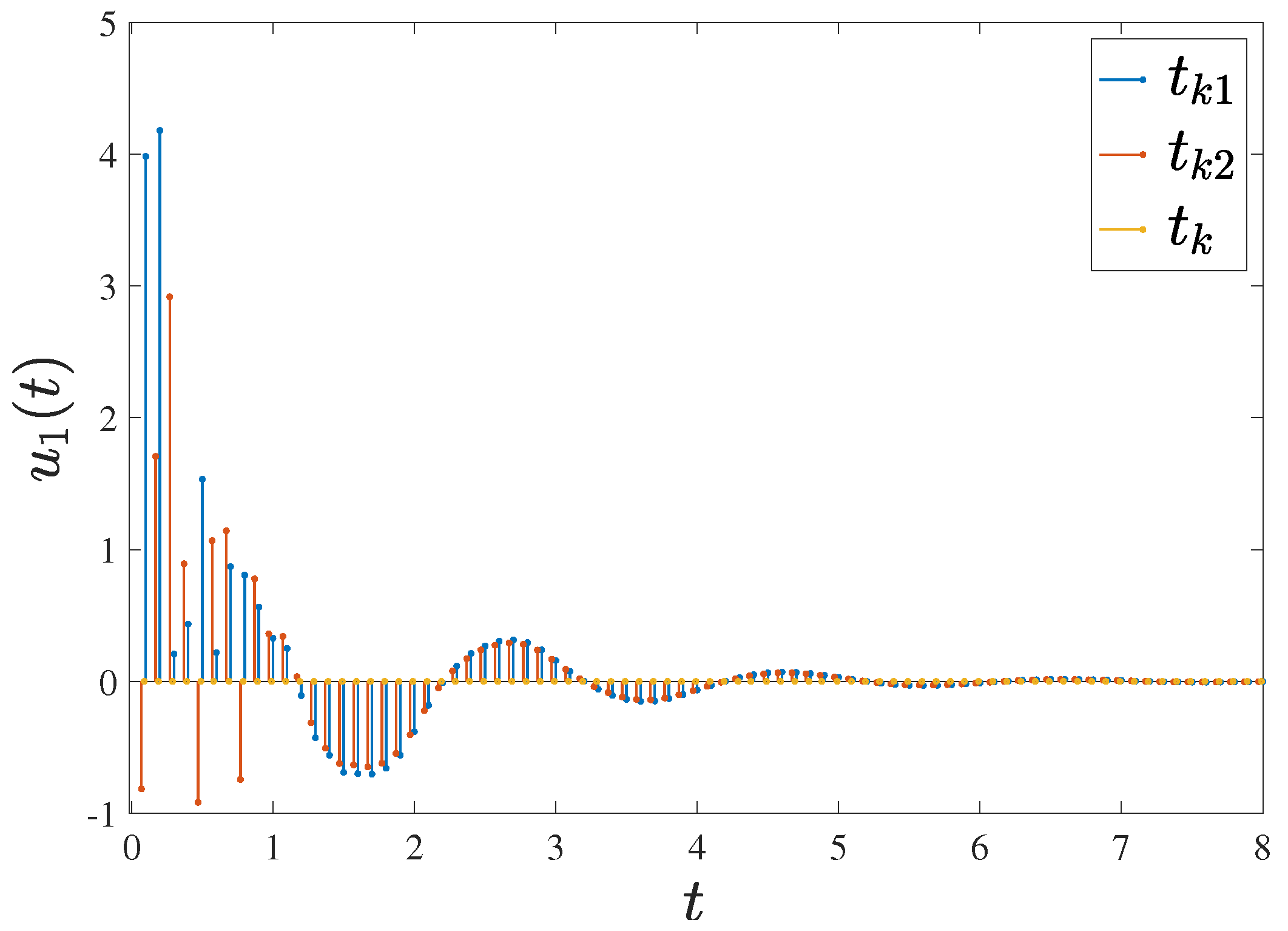
Letting , the control time is chosen as , the holding time is and the rest time is , as represented in Figure 3 and Figure 4. Furthermore, by selecting a delay of , FMNs (5) and (6) with controller (15) can achieve exponential synchronization, which is illustrated in Figure 5. The trajectories of error between FMNs (5) and (6) are below , which is consistent with the results of Theorem 1.
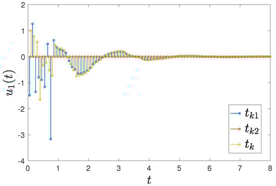
Figure 3.
The time interval with a control time of , holding time of and rest time of .
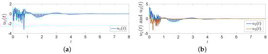
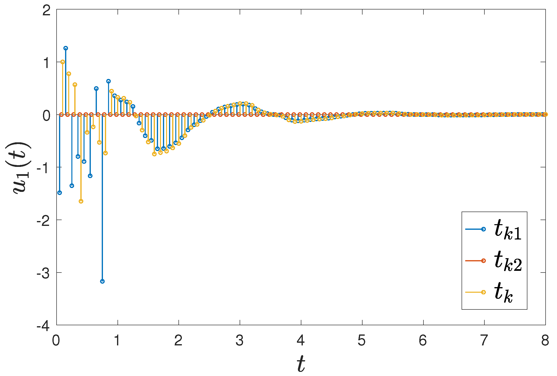
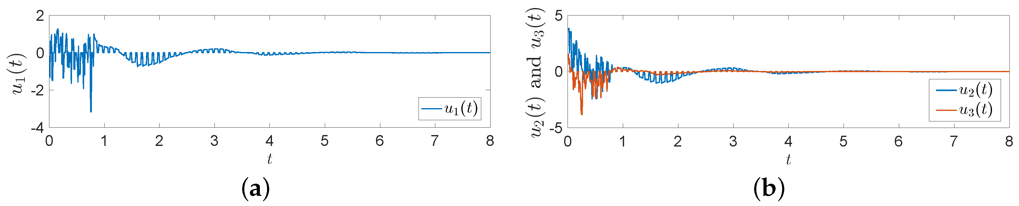
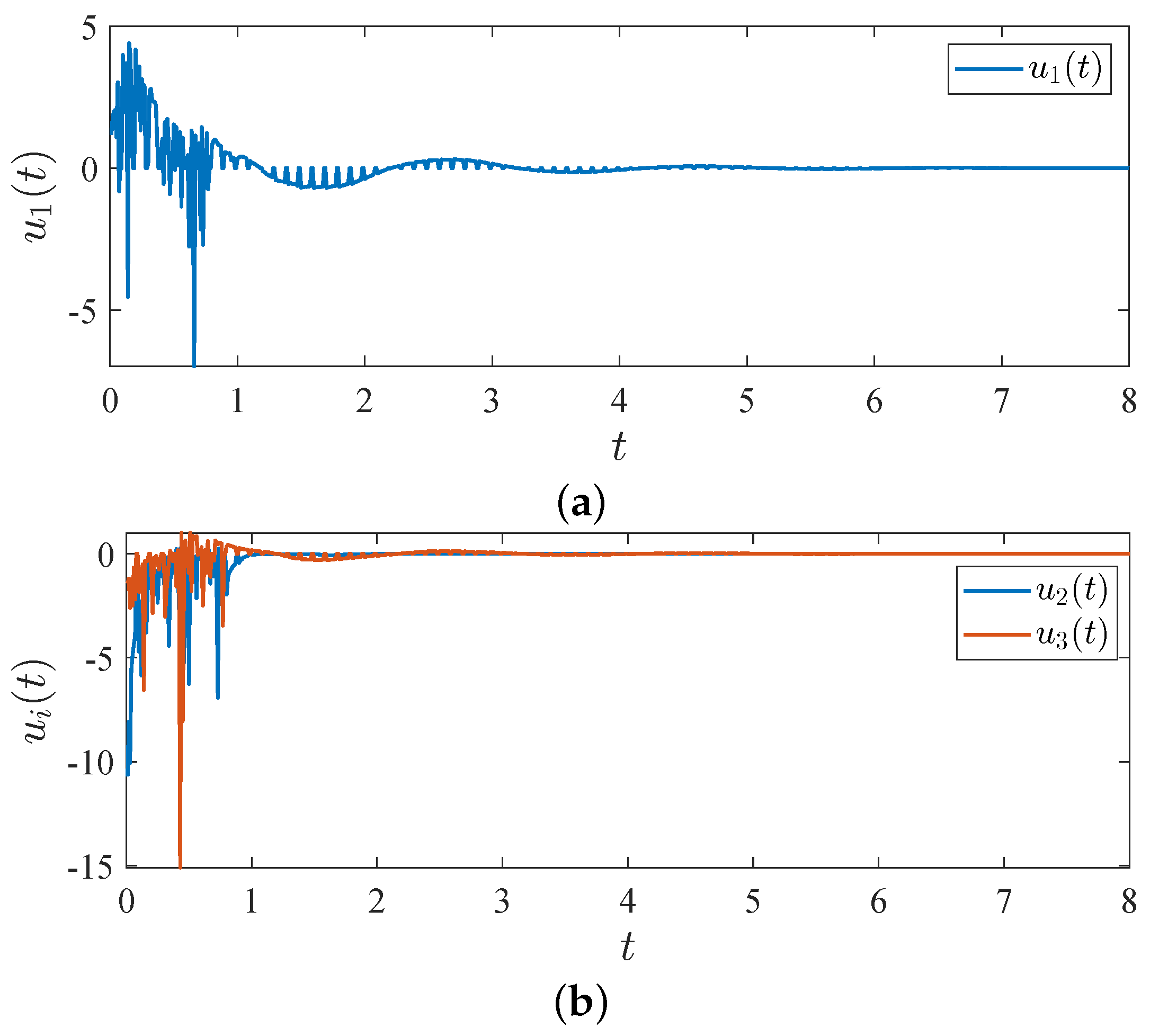
Figure 4.
Trajectories of controller (15) with a control time of , holding time of and rest time of . (a) ; (b) and .
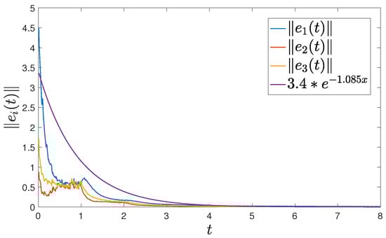
Figure 5.
The norm of error between FMNs (5) and (6) with .
To compare the performance of intermittent-hold control with that of traditional intermittent control, we compare convergence time using three different sets of initial values. The first set of initial values is and . The second set is and . The third set is and . The intermittent-hold controller becomes a traditional intermittent controller when the holding time is , letting , and .
Table 1 show that the intermittent-hold control strategy achieves a faster convergence rate than traditional intermittent control. Moreover, the intermittent-hold controller performs better than the traditional one when dealing with large time delays.

Table 1.
The error convergence time with different intermittent holding times and an error bound of .
Remark 5.
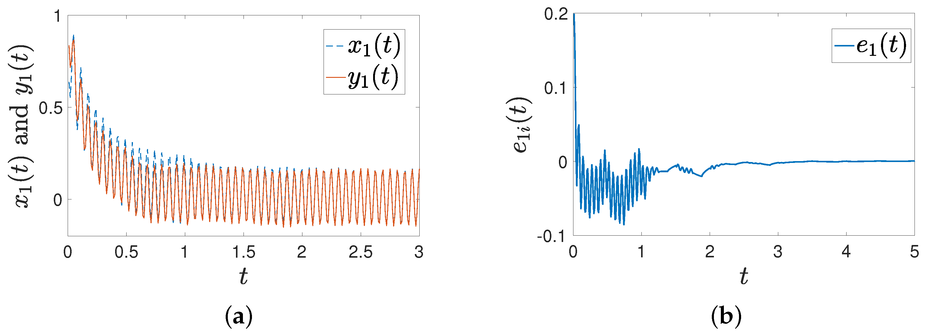
Based on the FO system parameters in Example 2 in [46], we can calculate that , , , , and , indicating that the presented results still work under the parameters reported in [46]. Figure 6 shows the synchronized states ( and ), along with the trajectories of error between two states. Under the parameters of Example 1 in [28], the theorems proposed in this paper are also valid. Moreover, the proposed results can be applied to handle larger delays, such as . Therefore, the results obtained in this paper are less conservative.
Figure 6.
Trajectories of states under the parameters reported in [46] with intermittent-hold control. (a) Trajectories of and ; (b) trajectories of error.
Example 2.
Consider a two-dimensional FMNN with a fuzzy cellular neural network with the following parameters:
where , , and and the activation functions are . Other parameters are denoted as follows:
Let and ; then, according to Lemma 2 and the above parameters, we can obtain
We can calculate that and , for , , . The control gains of controller (16) satisfy the conditions of Theorem 2 with the above system parameters. Therefore, the drive and response systems can achieve synchronization.
According to Theorem 2, we find that , , and . Figure 7 shows a control time of , a holding time of and a rest time of . To demonstrate the trajectory and effectiveness of the controller, we select three sets of states ( and ) with different initial values of , , , , and . Figure 8 shows the results obtain using the intermittent-hold controller integrated with an adaptive strategy and a delay of .
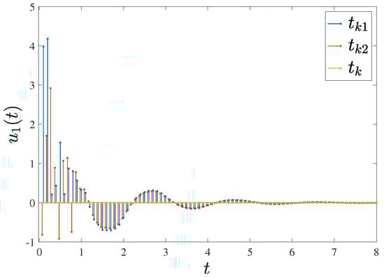
Figure 7.
The time interval with a control time of , a holding time of and a rest time of .

Figure 8.
Trajectories of controller (16) with three sets of states with different initial values and . (a) ; (b) and .
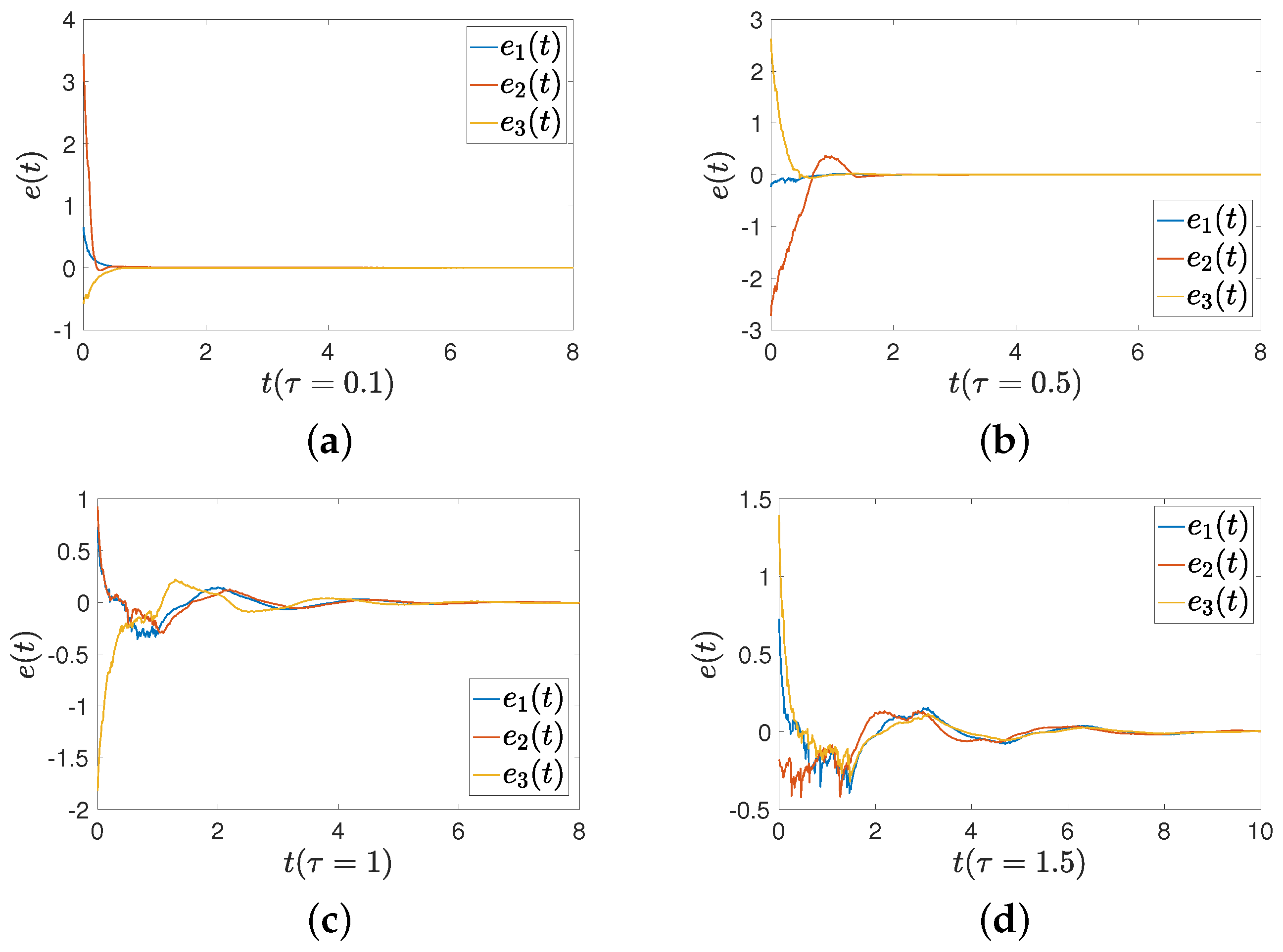
Figure 9 presents the error between drive and response systems based on three sets of states ( and ) with different initial values. is the first dimension of . Figure 9 shows that the conservation of Theorem 2 is reduced due to the application of intermittent-hold controller (16). In this simulation, we use three different initial values, with delays set to , , and . The errors between drive and response systems can converge to zero, which means that the results are applicable even in situations with larger delays.
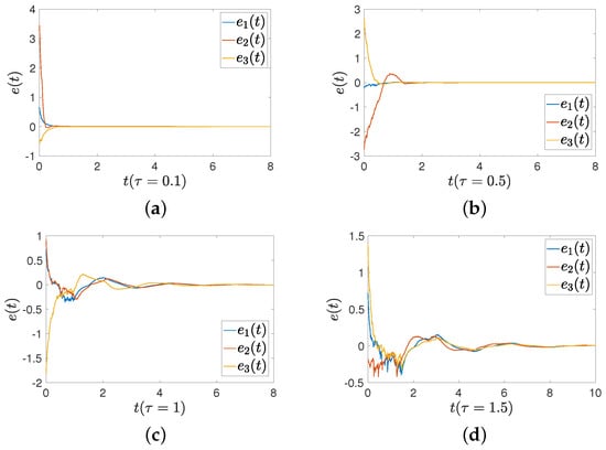
Figure 9.
The error between FMNs (5) and (6) under controller (16) with different delays. (a) Delay of ; (b) delay of ; (c) delay of ; (d) delay of .
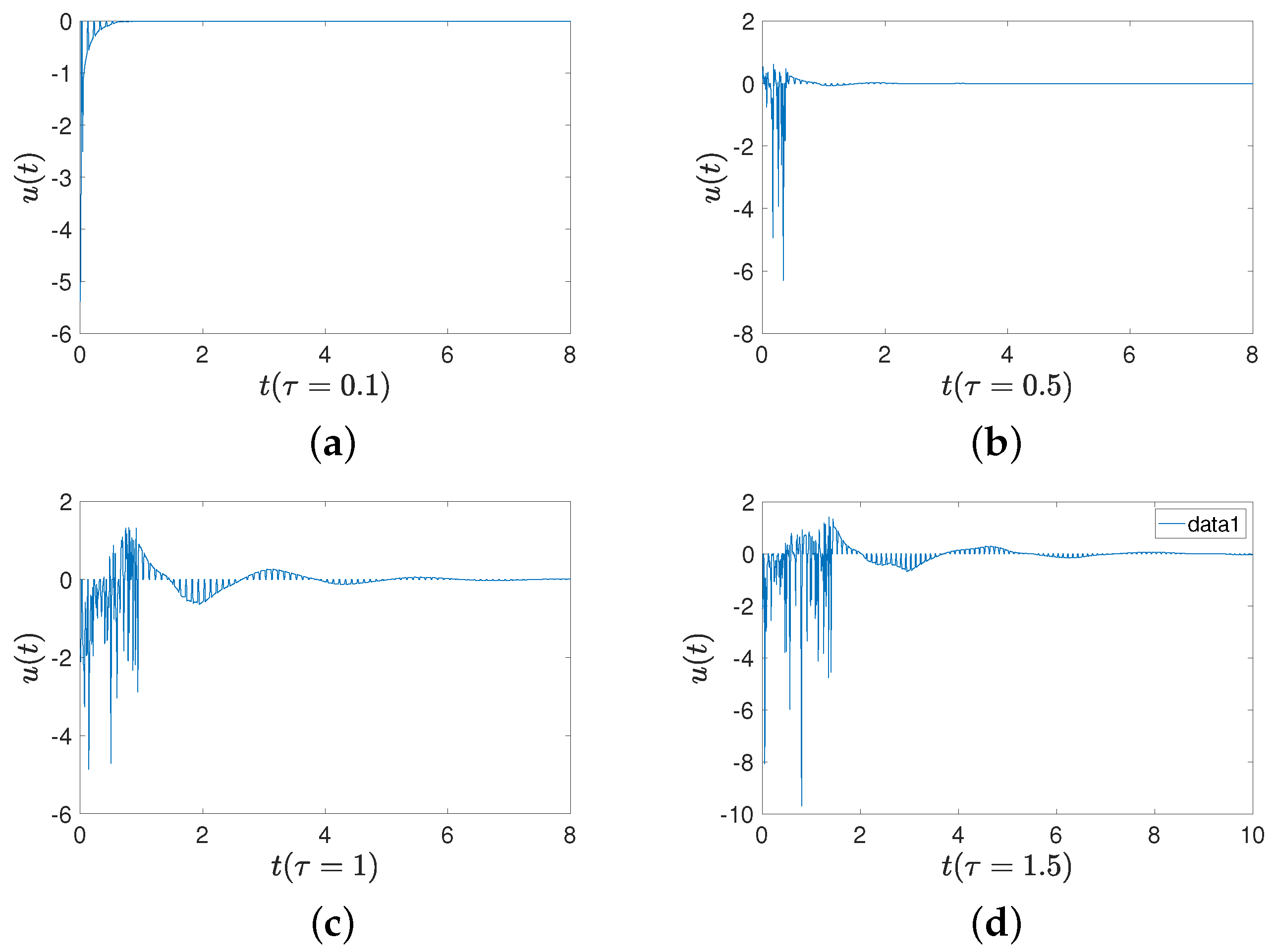
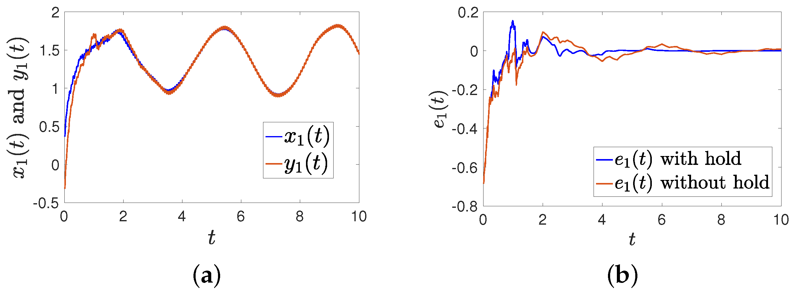
Figure 10 shows the trajectories of controller (16) with four different delays. The lager the time delays, the larger the controller adjustment range. Comparisons of convergence times for three sets of initial values are provided. The first set of initial values is and . The second set is and . The third set is and . Figure 11 shows a comparison between an intermittent-hold controller and a traditional intermittent controller. The delays are set as , , and Figure 11a shows that FMNs (5) and (6) can achieve synchronization, while Figure 11b displays the errors between two states under intermittent-hold control and intermittent control. Table 2 demonstrates that the intermittent-hold control strategy can converge faster than the traditional intermittent control.
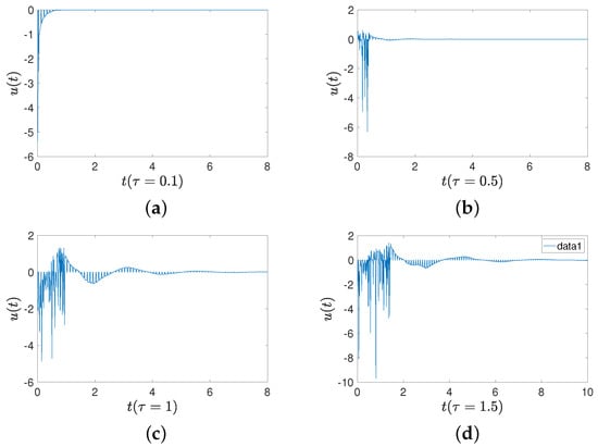
Figure 10.
Trajectories of controller (16) with different delays. (a) Delay of ; (b) delay of ; (c) delay of ; (d) delay of .
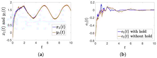
Figure 11.
Comparison of intermittent-hold control with traditional control (). (a) The trajectories of and with an intermittent hold controller; (b) the trajectories of error () with and without holding time.
Table 2.
The error converge time with different intermittent holding times and an error bound of .
Example 3.
Memristive neural networks can exhibit chaotic behaviors. Therefore, the results reported in this paper can be employed in secure communication problems.
System (1) can be degenerated as follows:
The memristive weights can be described as uncertainties, for instance, , , . The parameters are set as
and , , , , , , .
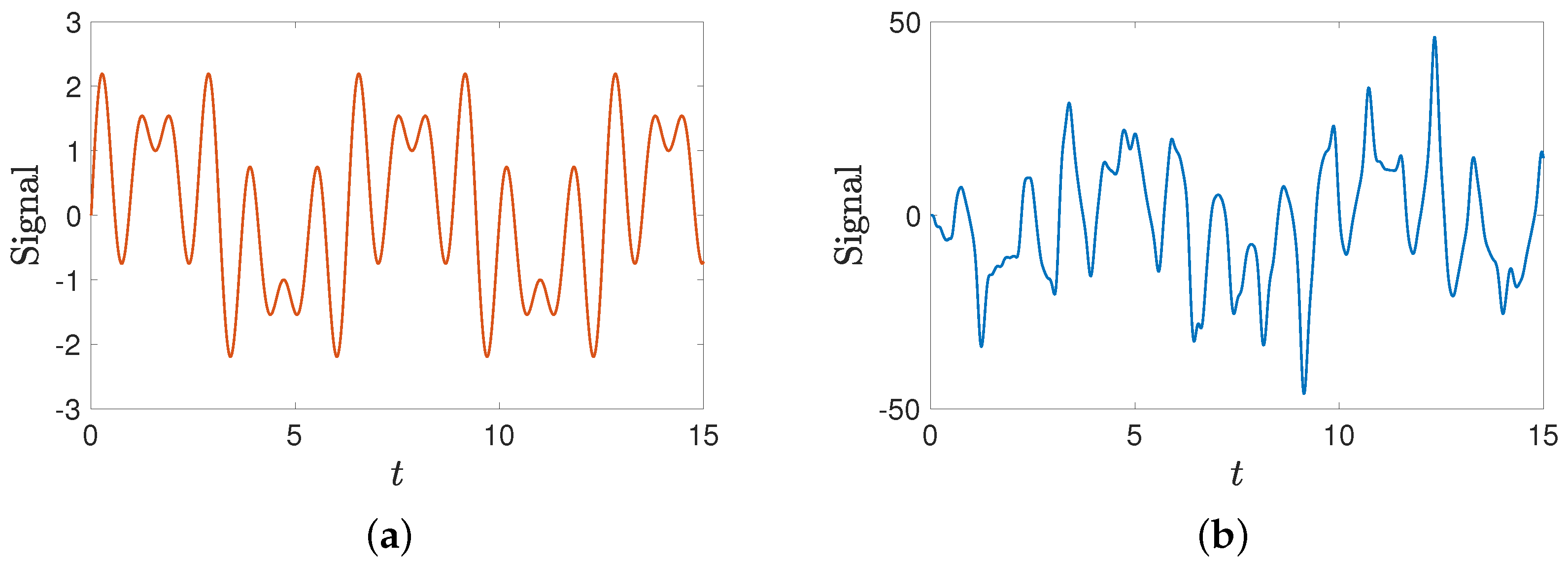
The response system has the same parameters. In the following simulation, the synchronization results are applied to the secure communication problem. First, the transmitter and receiver construct the same memristive neural networks to achieve signal synchronization. Based on Figure 12, we conclude that synchronization can be achieved by using controller (16). The transmitter combines the information signal with fractional-order MNN signals for encryption. The transmitted signal described as is shown in Figure 13a. The encryption function is , where and . The mixed signal is shown in Figure 13b.
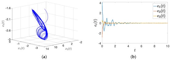
Figure 12.
States trajectory and synchronization. (a) The trajectories of ; (b) the trajectories of error with an intermittent hold controller.
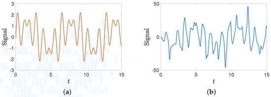
Figure 13.
The transmitted and encrypted information signals. (a) The transmitted information signal; (b) the mixed signal.
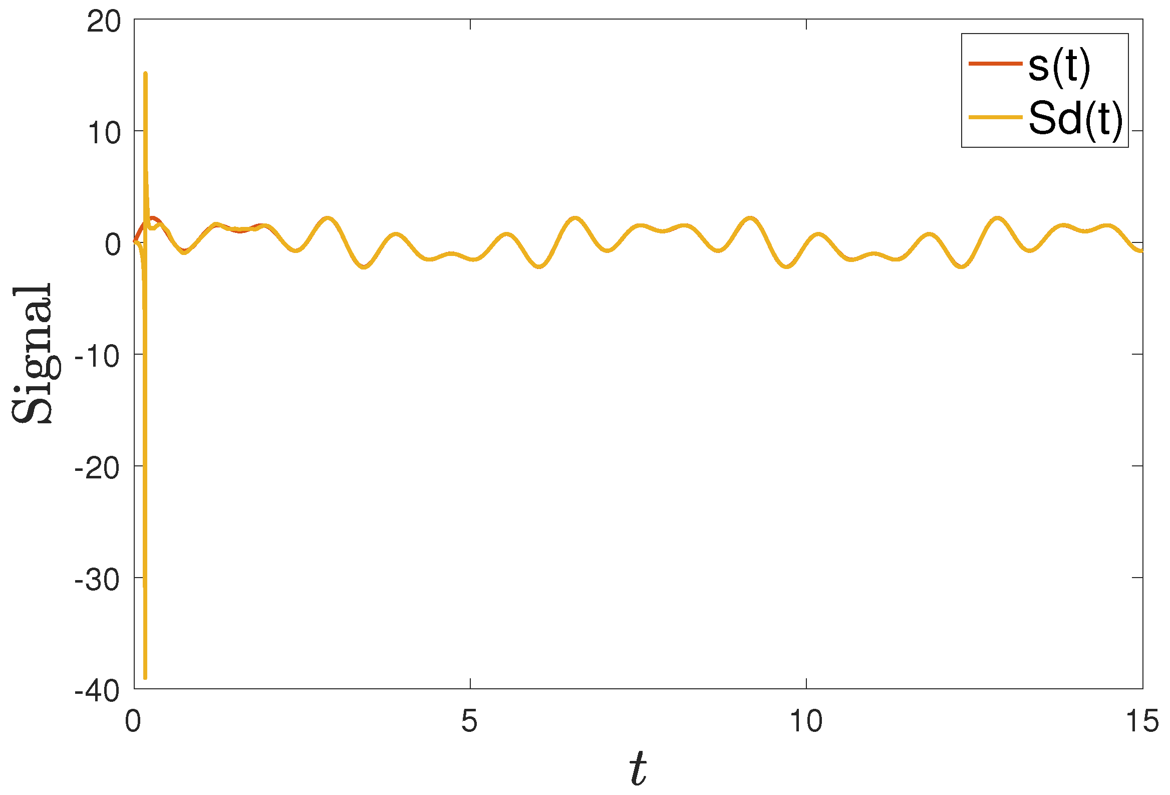
In this way, we can obtain the encryption signal (). The receiver uses the synchronized signal to recover the original signal as . Figure 14 shows that the signal can be decoded successfully.
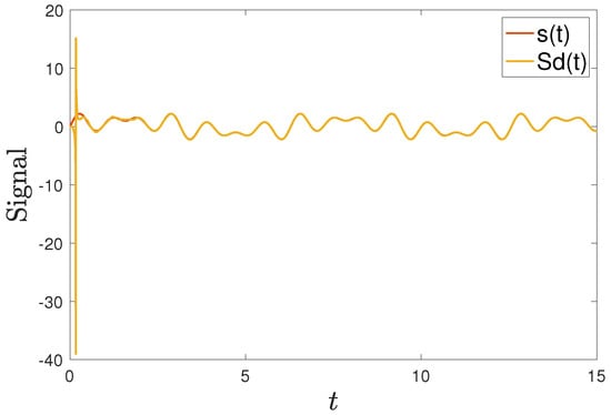
Figure 14.
The signal decrypted using the synchronization method.
Remark 6.
In the process of encryption and decryption through the use of the synchronization method, the initial errors are usually caused by the time required for the transmitter and receiver to establish synchronization. However, the two systems gradually adjust, reducing errors over time. These initial errors usually do not affect the long-term decryption effect because once the systems are synchronized, encryption and decryption can be proceed accurately, ensuring the security and reliability of information transmission.
5. Conclusions
In this paper, the exponential synchronization problems of FMFCNNs are investigated. A novel lemma is introduced to tackle the delay terms of FO systems via inequality techniques and the FO Laplace transform method. A new intermittent-hold controller is designed to address the synchronization problems. Furthermore, to handle more complicated situations, an intermittent-hold controller integrated with an adaptive control strategy is proposed. Additionally, two significant theorems are obtained on the basis of the proposed lemma and the two controllers. The simulation results confirm that the two proposed controllers can achieve exponential synchronization and effectively handle larger time delays. Compared with the traditional intermittent controllers, the proposed controllers have a faster convergence rate. Moreover, an application in secure communication is exhibited, which demonstrates the effectiveness of the results. For in future works, we will concentrate on the chaotic synchronization problems of FO systems.
Author Contributions
Conceptualization, X.Y.; Methodology, X.Y.; Writing—original draft, X.Y.; Data curation, J.S.; Software, J.S.; Validation, Y.D.; Supervision, S.Z.; Writing—review and editing, S.Z. and Y.D. All authors have read and agreed to the published version of the manuscript.
Funding
This work was financially supported by the Natural Science Foundation of Sichuan Province (Nos. 2023NSFSC1362 and 2023NSFSC0071), the Foundation of Chengdu University of Information Technology (No. KYTZ2022148), the 2023 Chengdu University of Information Technology Science and Technology Innovation Capability Enhancement Plan Innovation Team Key Project (KYTD202322) and the National Natural Science Foundation of China (No. 12101090).
Data Availability Statement
The generated datasets supporting the findings of this article are obtainable from the corresponding author upon reasonable request.
Conflicts of Interest
The authors declare no conflicts of interest.
Appendix A. Proof of Theorem 1
The proof is divided with three cases.
Case 1:
Consider the following Lyapunov function:
Then, taking the FO derivative of (A1), we have
According to Lemma 1 and Lemma 2, we can obtain
Together with the conditions of Theorem 1 (), we can obtain
where . According to Lemma 3, we have
that is,
Case 2:
Consider the following Lyapunov function:
Together with Lemma 1 and Lemma 2, taking the FO derivative of (A7), we can obtain
And we have following inequalities:
Substituting (A9) and (A10) into (A8), we can obtain
There exist and such that
Therefore, we have
where , and
According to Lemma 4 and the conditions of Theorem 1, we have
where , , , that is,
Case 3:
By using the same Lyapunov function, we have
where . Then, according to Lemma 4, we can obtain
where , that is,
Now, we can find that is bounded by an exponential decay function. For each time interval , we only need the minimum of for to be smaller than the minimum of for , that is,
For , we can find that the zero point of (7) is exponentially stable. This completes the proof.
Appendix B. Proof of Theorem 2
The proof is divided into three parts.
Case 1:
Consider the following Lyapunov function:
where
Because the controller used here is adaptive, the control gains are included in the construction of and . Then, taking the FO derivative of , according to the the proof of Theorem 1, we can obtain
Furthermore, we can find that
Taking the derivatives of and , we have
and
respectively.
According to (A23) to (A25) and the conditions of Theorem 2, we can obtain
where , , . Let ; then, we have
According to Lemma 3, we can obtain
Case 2:
Consider the following Laypunov function:
Then, we can obtain
There exist and such that
Substituting (A31) into (A30), we have
where , . According to Lemma 4, we can obtain
where , , .
Case 3:
By choosing the same Lyapunov function as (A29), we can obtain
According to Lemma 4, we can obtain
where , , . In the same way as Theorem 1, we can find that is bounded by an exponential decay function. This completes the proof.
References
- Chua, L.O. Memristor-The missing circuit element. IEEE Trans. Circuit Theory 1971, 18, 507–519. [Google Scholar] [CrossRef]
- Strukov, D.; Snider, G.; Stewart, D.; Williams, R. The missing memristor found. Nature 2008, 453, 80–83. [Google Scholar] [CrossRef] [PubMed]
- Patro, P.; Kumar, K.; Kumar, G.S. Cellular Neural Network, Fuzzy Cellular Neural Networks and its Applications. Int. J. Control Theory Appl. 2017, 10, 161–167. [Google Scholar]
- Wu, Z.; Zhang, C.; Zou, J.; Peng, C.; Wu, X. Threshold switching memristor-based voltage regulative circuit. IEEE Trans. Circuits Syst. II Express Briefs 2023, 70, 1034–1038. [Google Scholar] [CrossRef]
- Min, F.; Xue, L. Routes toward chaos in a memristor-based shinriki circuit. Chaos 2023, 33, 023122. [Google Scholar] [CrossRef]
- Bao, H.; Liu, W.; Hu, A. Coexisting multiple firing patterns in two adjacent neurons coupled by memristive electromagnetic induction. Nonlinear Dyn. 2019, 95, 43–56. [Google Scholar] [CrossRef]
- Lin, H.; Wang, C.; Hong, Q.; Sun, Y. A multi-stable memristor and its application in a neural network. IEEE Trans. Circuits Syst. II Express Briefs 2020, 67, 3472–3476. [Google Scholar] [CrossRef]
- Qin, X.; Wang, C.; Li, L.; Peng, H.; Ye, L. Finite-time lag synchronization of memristive neural networks with multi-links via adaptive control. IEEE Access 2020, 8, 55398–55410. [Google Scholar] [CrossRef]
- Qi, A.; Zhu, B.; Wang, G. Complex dynamic behaviors in hyperbolic-type memristor-based cellular neural network. Chin. Phys. B 2022, 31, 020502. [Google Scholar] [CrossRef]
- Lin, H.; Wang, C.; Sun, J.; Zhang, X.; Sun, Y.; Iu, H. Memristor-coupled asymmetric neural networks: Bionic modeling, chaotic dynamics analysis and encryption application. Chaos Solitons Fractals 2023, 166, 112905. [Google Scholar] [CrossRef]
- Chua, L.O.; Yang, L. Cellular Neural Network: Theory. IEEE Trans. Circuits Syst. 1988, 35, 1257–1272. [Google Scholar] [CrossRef]
- Wang, P.; Li, X.; Wang, N.; Li, Y.; Shi, K.; Lu, J. Almost periodic synchronization of quaternion-valued fuzzy cellular neural networks with leakage delays. Fuzzy Sets Syst. 2022, 426, 46–65. [Google Scholar] [CrossRef]
- Guo, Y.; Ge, S.; Arbi, A. Stability of traveling waves solutions for nonlinear cellular neural networks with distributed delays. J. Syst. Sci. Complex. 2022, 35, 18–31. [Google Scholar] [CrossRef]
- Kashkynbayev, A.; Issakhanov, A.; Otkel, M.; Kurths, J. Finite-time and fixed-time synchronization analysis of shunting inhibitory memristive neural networks with time-varying delays. Chaos Solitons Fractals 2022, 156, 111866. [Google Scholar] [CrossRef]
- Yang, T.; Yang, L.; Wu, C.; Chua, L.O. Fuzzy cellular neural networks: Theory. In Proceedings of the 1996 Fourth IEEE International Workshop on Cellular Neural Networks and Their Applications Proceedings (CNNA-96), Seville, Spain, 24–26 June 1996; pp. 181–186. [Google Scholar]
- Yang, T.; Yang, L. The global stability of fuzzy cellular neural network. IEEE Trans. Circuits Syst. I 1966, 43, 880–883. [Google Scholar] [CrossRef]
- Liu, D.; Wang, L.; Pan, Y.; Ma, H. Mean square exponential stability for discrete-time stochastic fuzzy neural networks with mixed time-varying delay. Neurocomputing 2016, 171, 1622–1628. [Google Scholar] [CrossRef]
- Guo, Z.; Wang, J.; Yan, Z. Attractivity Analysis of Memristor-Based Cellular Neural Networks With Time-Varying Delays. IEEE Trans. Neural Netw. Learn. Syst. 2013, 25, 704–717. [Google Scholar] [CrossRef]
- Zheng, M.; Li, L.; Peng, H.; Xiao, J.; Yang, Y.; Zhang, Y. Fixed-time synchronization of memristive fuzzy BAM cellular neural networks with time-varying delays based on feedback controllers. IEEE Access 2018, 6, 12085–12102. [Google Scholar] [CrossRef]
- Zheng, M.; Li, L.; Peng, H.; Xiao, J.; Yang, Y.; Zhang, Y.; Zhao, H. Fixed-time synchronization of memristor-based fuzzy cellular neural network with time-varying delay. J. Frankl. Inst. 2018, 355, 6780–6809. [Google Scholar] [CrossRef]
- Kaslik, E.; Sivasundaram, S. Dynamics of fractional-order neural networks. In Proceedings of the 2011 International Joint Conference on Neural Networks, San Jose, CA, USA, 31 July–5 August 2011; pp. 611–618. [Google Scholar]
- Radwan, A.; Emira, A.; AbdelAty, A.; Azar, A. Modeling and analysis of fractional order DC-DC converter. ISA Trans. 2018, 82, 184–199. [Google Scholar] [CrossRef]
- Stamova, I.; Stamov, G. Mittag-leffler synchronization of fractional neural networks with time-varying delays and reaction–diffusion terms using impulsive and linear controllers. Neural Netw. 2017, 96, 22–32. [Google Scholar] [CrossRef] [PubMed]
- Arena, P.; Caponetto, R.; Fortuna, L.; Porto, D. Bifurcation and chaos in noninteger order cellular neural networks. Int. J. Bifurc. Chaos 1998, 8, 1527–1539. [Google Scholar] [CrossRef]
- Ma, W.; Li, C.; Wu, Y.; Wu, Y. Synchronization of fractional fuzzy cellular neural networks with interactions. Chaos Interdiscip. J. Nonlinear Sci. 2017, 27, 103106. [Google Scholar] [CrossRef] [PubMed]
- Petráš, I. Fractional-order memristor-based chua’s circuit. IEEE Trans. Circuits Syst. II Express Briefs 2010, 57, 975–979. [Google Scholar]
- Syed, A.; Narayanan, G.; Saroha, S.; Priya, B.; Thakur, G. Finite-time analysis of fractional-order memristive fuzzy cellular networks with time delay and leakage term. Math. Comput. Simul. 2021, 185, 468–485. [Google Scholar] [CrossRef]
- Zheng, M.; Li, L.; Peng, H.; Xiao, J.; Yang, Y.; Zhang, Y.; Zhao, H. Finite-time stability and synchronization of memristor-based fractional-order fuzzy cellular neural networks. Commun. Nonlinear Sci. Numer. Simul. 2018, 59, 272–291. [Google Scholar] [CrossRef]
- Sun, Y.; Liu, Y. Fixed-time synchronization of delayed fractional-order memristor-based fuzzy cellular neural networks. IEEE Access 2020, 8, 165951–165962. [Google Scholar] [CrossRef]
- Saifia, D.; Chadli, M.; Labiod, S.; Cuerra, T. Robust H∞ static output-feedback control for discrete-time fuzzy systems with actuator saturation via fuzzy Lyapunov functions. Asian J. Control 2020, 22, 611–623. [Google Scholar] [CrossRef]
- Li, D.; Liu, Y.; Tong, S.; Chen, C.; Li, D. Neural networks-based adaptive control for nonlinear state constrained systems with input delay. IEEE Trans. Cybern. 2018, 49, 1249–1258. [Google Scholar] [CrossRef]
- Zhang, T.; Zhou, J.; Liao, Y. Exponentially stable periodic oscillation and Mittag–Leffler stabilization for fractional-order impulsive control neural networks with piecewise Caputo derivatives. IEEE Trans. Cybern. 2021, 52, 9670–9683. [Google Scholar] [CrossRef]
- Zhou, Y.; Zhang, H.; Zeng, Z. Synchronization of memristive neural networks with unknown parameters via event-triggered adaptive control. Neural Netw. 2021, 139, 255–264. [Google Scholar] [CrossRef] [PubMed]
- Cheng, L.; Qiu, J.; Chen, X.; Zhang, A.; Yang, C.; Chen, X. Adaptive aperiodically intermittent control for pinning synchronization of directed dynamical networks. Int. J. Robust Nonlinear Control 2019, 29, 1909–1925. [Google Scholar] [CrossRef]
- Fan, Y.; Huang, X.; Li, Y.; Xia, J.; Chen, G. Aperiodically intermittent control for quasi-synchronization of delayed memristive neural networks: An interval matrix and matrix measure combined method. IEEE Trans. Syst. Man Cybern. Syst. 2018, 49, 2254–2265. [Google Scholar] [CrossRef]
- Chen, T.; Wang, F.; Xia, C.; Chen, Z. Leader-following consensus of second-order multi-agent systems with intermittent communication via persistent-hold control. Neurocomputing 2022, 471, 183–193. [Google Scholar] [CrossRef]
- Liu, C.; Zhang, Y.; Chen, Y. Persistent-hold consensus control of First-order multi-agent systems with intermittent communication. In Proceedings of the 23rd International Symposium on Mathematical Theory of Networks and Systems, Hong Kong, China, 16–20 July 2018. [Google Scholar]
- Xiu, C.; Zhou, R.; Liu, Y. New chaotic memristive cellular neural network and its application in secure communication system. Chaos Solitons Fractals 2020, 141, 110316. [Google Scholar] [CrossRef]
- Kekha Javan, A.A.; Zare, A.; Alizadehsani, R.; Balochian, S. Robust multi-mode synchronization of chaotic fractional order Systems in the Presence of disturbance, time delay and uncertainty with application in secure communications. Big Data Cogn. Comput. 2022, 6, 51. [Google Scholar] [CrossRef]
- Gokyildirim, A.; Akgul, A.; Calgan, H.; Demirtas, M. Parametric fractional-order analysis of Arneodo chaotic system and microcontroller-based secure communication implementation. Int. J. Electron. Commun. 2024, 175, 155080. [Google Scholar] [CrossRef]
- Podlubny, I. Fractional Differential Equations; Academic Press: San Diego, CA, USA, 1999. [Google Scholar]
- Chen, J.; Zeng, Z.; Jiang, P. Global Mittag-Leffer stability and synchronization of memristor-based fractional-order neural networks. Neural Netw. 2014, 51, 1–8. [Google Scholar]
- Jian, J.; Wan, P. Lagrange α-exponential stability and α-exponential convergence for fractional-order complex-valued neural networks. Neural Netw. 2017, 91, 1–10. [Google Scholar] [CrossRef]
- Liu, C.; Liu, S.; Zhang, Y.; Chen, Y. Consensus seeking of multi-agent systems with intermittent communication: A persistent-hold control strategy. Int. J. Control 2020, 93, 2161–2167. [Google Scholar] [CrossRef]
- Wang, D.; Xiao, A. Dissipativity and contractivity for fractional-order systems. Nonlinear Dyn. 2015, 80, 287–294. [Google Scholar] [CrossRef]
- Chen, L.; Cao, J.; Wu, R.; Tenreiro Machado, J.A.; Lopes, A.M.; Yang, H. Stability and sychronization of fractional-order memristive neural networks with multiple delays. Neural Netw. 2017, 94, 76–85. [Google Scholar] [CrossRef] [PubMed]
Disclaimer/Publisher’s Note: The statements, opinions and data contained in all publications are solely those of the individual author(s) and contributor(s) and not of MDPI and/or the editor(s). MDPI and/or the editor(s) disclaim responsibility for any injury to people or property resulting from any ideas, methods, instructions or products referred to in the content. |
© 2024 by the authors. Licensee MDPI, Basel, Switzerland. This article is an open access article distributed under the terms and conditions of the Creative Commons Attribution (CC BY) license (https://creativecommons.org/licenses/by/4.0/).