Iterated Relation Systems on Riemannian Manifolds

Abstract

For fractals on Riemannian manifolds, the theory of iterated function systems often does not apply well directly, as these fractal sets are often defined by relations that are multivalued or non-contractive. To overcome this difficulty, we introduce the novel notion of iterated relation systems. We study the attractor of an iterated relation system and formulate a condition under which such an attractor can be identified with that of an associated graph-directed iterated function system. Using this method, we obtain dimension formulas for the attractor of an iterated relation system on locally Euclidean Riemannian manifolds, under the graph open set condition or the graph finite type condition. This method improves the one by Ngai and Xu, which relies on knowing the specific structure of the attractor. We also study fractals generated by iterated relation systems on Riemannian manifolds that are not locally Euclidean.

1. Introduction

Fractals in Riemannian manifolds, especially in Lie groups, Heisenberg groups, and projective spaces, have been studied extensively by many authors (see Strichartz [1], Balogh and Tyson [2], Barnsley and Vince [3], Hossain et al. [4,5], etc.). A basic theory of iterated function systems (IFSs) on Riemannian manifolds, including Hausdorff dimension, the weak separation condition (WSC), and the finite type condition (FTC), was established by Xu and the second author [6]. In [6], a method for computing the Hausdorff dimension of a certain fractal set in a flat torus is obtained; the fractal set can be identified with the attractor of some IFS on ${\mathbb{R}}^2/{\mathbb{Z}}^2$. However, this method is too cumbersome and is not easy to generalize. The purpose of this paper is to establish a new method that can be used to calculate the Hausdorff dimensions of more general fractal sets in Riemannian manifolds. Unlike fractal sets in ${\mathbb{R}}^n$, many interesting fractals in Riemannian manifolds cannot be described by an IFS. For example, the relations generating a Sierpinski gasket on a cylinder can be multivalued (see Example 4). Thangaraj et al. [7] studied fractals generated by multivalued functions in a metric space. Cui et al. [8] studied measures generated by nonautonomous iterated function systems consisting of expansive maps. Unlike mappings in these papers, relations that generate fractals considered in the present paper can be multivalued and expansive at the same time. To deal with the problem that the maps (or more precisely, relations) generating a fractal are multivalued and non-contractive, we introduce the notion of iterated relation systems (IRSs) (see Definition 1). We show that many interesting fractals can be described naturally by IRSs.

Let ${\left\{R_t\right\}}_{t=1}^N$ be an IRS on a nonempty compact subset of a topological space, and let K be the attractor of ${\left\{R_t\right\}}_{t=1}^N$ (see Definition 2). Then

$$\begin{array}{c}\hfill K=\bigcup _{t=1}^N{R}_t\left(K\right)\end{array}$$

(1)

(see Proposition 2). However, in general, a nonempty compact set K satisfying (1) need not be unique and, therefore, need not be the attractor of ${\left\{R_t\right\}}_{t=1}^N$; Example A2 illustrates this. To study the uniqueness of K, we introduce the notion of a graph-directed iterated function system (GIFS) associated with an IRS (see Definition 4), and prove the uniqueness of K under the assumption that such a GIFS exists.

Since relations need not be single-valued or contractive, it might not be possible to construct a GIFS associated with an IRS (see Examples A3 and A4). Our first goal is to study, under suitable conditions, the existence of a GIFS associated with an IRS (see Theorem 1).

In Section 5, we study IRS attractors under the assumption that an associated GIFS satisfies (GOSC). Our second goal is to describe a method for computing the Hausdorff dimension of an IRS attractor in a Riemannian manifold under the assumption that an associated GIFS G exists and G satisfies (GOSC).

It is worth pointing out that Balogh and Rohner [9] extended the Moran–Hutchinson theorem (see [10]) to the more general setting of doubling metric spaces. Wu and Yamaguchi [11] generalized the results of Balogh and Rohner.

For IFSs on ${\mathbb{R}}^n$, the finite type was first introduced by Wang and the second author [12], and was extended to the general finite type condition independently by Jin and Yau [13], and Lau and the second author [14]. The graph finite type condition (GFTC) was extended to Riemannian manifolds by Xu and the second author [6]. In Section 6, we study IRS attractors under the assumption that a GIFS associated with an IRS satisfies (GFTC). Our third goal is to obtain a method for computing the Hausdorff dimension of the attractor that improves the one in [6].

Fractals on spheres have, in fact, been studied quite extensively, especially in connection with the stereographic metric and comparison of dimensions (see [15]), construction of fractal functions on the sphere (see [16,17]), and IFSs consisting of Möbius transformations (see [18]). In Section 7, we study fractals generated by IRSs on spheres. Computing the dimension of an attractor becomes substantially harder, as the sphere is not locally Euclidean. Nevertheless, we show in Example 6 how to obtain the box dimension.

This paper is organized as follows. In Section 2, we state our main theorems. In Section 3, we give the definition of an IRS and study the properties of its attractor. Section 4 is devoted to the proof of Theorem 1. In Section 5, we prove Theorems 2–3. We also construct an IRS satisfying the conditions of Theorem 3, and compute the Hausdorff dimension of the associated attractors. In Section 6, we prove Theorems 4–5 and provide examples to illustrate Theorem 5. In Section 7, we study fractals generated by iterated relation systems on ${\mathbb{S}}^2$, which is not locally Euclidean. Finally, a conclusion is given in Section 8.

2. Statement of Main Results

This section contains the statements of our main theorems. The proofs of these theorems are presented later in the paper, as we need to first establish some basic theory.

Let $\#F$ be the cardinality of a set F. The definition of a finite family of contractions decomposed from ${\left\{R_t\right\}}_{t=1}^N$ and the definition of a good partition that appear in our first main theorem below are given in Definition 5.

Theorem 1.

Let X be a complete metric space, and let $E_0\subseteq X$ be a nonempty compact set. Let ${\left\{R_t\right\}}_{t=1}^N$ ($N\ge 1$) be an IRS on $E_0$. For any integer $k\ge 0$, let $E_{k+1}:={\bigcup }_{t=1}^N{R}_t\left(E_k\right)$. Assume that ${\left\{R_t\right\}}_{t=1}^N$ satisfies the following conditions:

(a) 

There exists an integer $k_0\ge 1$ such that for any $t\in \{1,\dots ,N\}$ and any $x\in E_{k_0-1}$,

$$\#\left\{R_t\left(x\right)\right\}<\infty .$$

(b) 

For any $t\in \{1,\dots ,N\}$, if $H_t:=\{x\in E_{k_0-1}:2\le \#\left\{R_t\left(x\right)\right\}<\infty \}\ne Ø$, we require that the following conditions are satisfied:

(i) 

$r_t:=R_t{|}_{H_t}$ can be decomposed as a finite family of contractions ${\{h_t^{l,i}:H_t^i\to h_t^{l,i}\left(H_t^i\right)\}}_{l=1,i=1}^{n_t,m_t}$, where ${\bigcup }_{i=1}^{m_t}{H}_t^i=H_t$, and ${\tilde{r}}_t:=R_t{|}_{E_{k_0-1}\setminus H_t}$ can be decomposed as a finite family of contractions ${\{h_t^{0,i}:J_t^i\to h_t^{0,i}\left(J_t^i\right)\}}_{i=1}^{q_t}$, where ${\bigcup }_{i=1}^{q_t}{J}_t^i=E_{k_0-1}\setminus H_t$.

(ii) 

There exists a good partition on $E_{k_0}$ with respect to some finite family of contractions decomposed from ${\left\{R_t\right\}}_{t=1}^N$ (not necessarily the one in $\left(i\right)$).

Then there exists a GIFS associated to ${\left\{R_t\right\}}_{t=1}^N$ on $E_{k_0}$.

We give examples (see Examples A3–A6) to investigate the conditions in Theorem 1. Under the assumption that ${\left\{R_t\right\}}_{t=1}^N$ satisfies conditions (a) and (b) (i) in Theorem 1, we give a sufficient condition for the hypothesis (b) (ii) to be satisfied (see Theorem 6).

The construction of the incidence matrices that appear in Theorems 2–3 will be given in Section 5 (see (22)).

Theorem 2.

Let M be a complete n-dimensional smooth orientable Riemannian manifold that is locally Euclidean. Let ${\left\{R_t\right\}}_{t=1}^N$ be an IRS on a nonempty compact subset of M, and K be the associated attractor. Assume that there exists a GIFS $G=(V,E)$ associated with ${\left\{R_t\right\}}_{t=1}^N$, and assume that G consists of contractive similitudes. Suppose that G satisfies (GOSC). Let ${\lambda }_{\alpha }$ be the spectral radius of the incidence matrix $A_{\alpha }$ associated with G. Then

$${dim}_{\mathrm{H}}\left(K\right)=\alpha ,$$

where α is the unique number such that ${\lambda }_{\alpha }=1$.

The definitions of a simplified GIFS and a minimal simplified GIFS are given in Definitions 6 and 7, respectively.

Theorem 3. 

Let M, ${\left\{R_t\right\}}_{t=1}^N$, K, and $G=(V,E)$ be as in Theorem 2. Let $\widehat{G}=(\widehat{V},\widehat{E})$ be a minimal simplified GIFS associated with G. Assume that $\widehat{G}$ satisfies (GOSC). Let ${\widehat{\lambda }}_{\alpha }$ be the spectral radius of the incidence matrix ${\widehat{A}}_{\alpha }$ associated with $\widehat{G}$.

(a) 

${dim}_{\mathrm{H}}\left(K\right)=\alpha$, where α is the unique real number such that ${\widehat{\lambda }}_{\alpha }=1$.

(b) 

In particular, let $\widehat{G}=(\widehat{V},\widehat{E})$ be a minimal simplified GIFS associated with G and assume that $\widehat{G}$ consists of contractive similitudes ${\left\{f_t\right\}}_{t=1}^m$. Suppose that $\#\widehat{V}=1$. If ${\left\{f_t\right\}}_{t=1}^m$ satisfies (OSC), then ${dim}_{\mathrm{H}}\left(K\right)$ is the unique number α satisfying

$$\sum _{t=1}^m{\rho }_t^{\alpha }=1,$$

where ${\rho }_t$ is the contraction ratio of $f_t$.

The construction of the weighted incidence matrices that appear in the following theorems is given in Section 6.

Theorem 4. 

Let M, ${\left\{R_t\right\}}_{t=1}^N$, K, and $G=(V,E)$ be as in Theorem 2. Assume that G satisfies (GFTC). Let ${\lambda }_{\alpha }$ be the spectral radius of the weighted incidence matrix $A_{\alpha }$ associated with G. Then

$${dim}_{\mathrm{H}}\left(K\right)=\alpha ,$$

where α is the unique real number such that ${\lambda }_{\alpha }=1$.

Theorem 5. 

Let M, ${\left\{R_t\right\}}_{t=1}^N$, K, and $G=(V,E)$ be as in Theorem 2. Let $\widehat{G}=(\widehat{V},\widehat{E})$ be a minimal simplified GIFS associated with G. Assume that $\widehat{G}$ satisfies (GFTC). Let ${\widehat{\lambda }}_{\alpha }$ be the spectral radius of the weighted incidence matrix ${\widehat{A}}_{\alpha }$ associated with $\widehat{G}$. Then

$${dim}_{\mathrm{H}}\left(K\right)=\alpha ,$$

where α is the unique real number such that ${\widehat{\lambda }}_{\alpha }=1$.

3. Iterated Relation Systems

Throughout this paper, we let $\Sigma :=\{1,\dots ,N\}$, where $N\in \mathbb{N}$. We first introduce the definition of an IRS.

Definition 1. 

Let T be a topological space and let $E_0\subseteq T$ be a nonempty compact set. Let ${\left\{R_t\right\}}_{t=1}^N$ be a family of relations defined on $E_0$. For any integer $n\ge 0$, let

$$\begin{array}{c}\hfill E_{n+1}:=\bigcup _{t=1}^N{R}_t\left(E_n\right).\end{array}$$

(2)

We call ${\left\{R_t\right\}}_{t=1}^N$ an iterated relation system (IRS) if it satisfies the following conditions:

(a) 

for any nonempty compact set $F\subseteq E_0$ and $t\in \Sigma$, $R_t\left(F\right)$ is a nonempty compact set;

(b) 

for any $t\in \Sigma$, $R_t\left(E_0\right)\subseteq E_0$.

Examples 1, 2–4, and 5–6 illustrate IRSs with various properties.

Proposition 1. 

Let T be a topological space, and let $E_0\subseteq T$ be a nonempty compact set. Let ${\left\{R_t\right\}}_{t=1}^N$ be an IRS on $E_0$. For any integer $n\ge 0$, let $E_n$ be defined as in (2). Then ${\bigcap }_{n=0}^{\infty }{E}_n$ is a nonempty compact set.

Proof. 

By Definition 1 (b), we have $E_1\subseteq E_0$. Assume that $E_{n+1}\subseteq E_n$ for some $n\ge 0$. Then

$$\begin{array}{cc}\hfill E_{n+2}& =\bigcup _{t=1}^N{R}_t\left(E_{n+1}\right)\subseteq \bigcup _{t=1}^N{R}_t\left(E_n\right)=E_{n+1}.\hfill \end{array}$$

Hence, for any $n\ge 0$, $E_{n+1}\subseteq E_n$. We know that $E_0$ is a nonempty compact set. Assume that $E_n$ is a nonempty compact set for some $n\ge 1$. By Definition 1 (a), $R_t\left(E_n\right)$ is a nonempty compact set for any $t\in \Sigma$. Hence, $E_{n+1}$ is a nonempty compact set. Therefore, ${\left\{E_n\right\}}_{n=0}^{\infty }$ is a decreasing sequence of nonempty compact subsets of T. This proves the proposition.  □

Definition 2.

Let T, $E_0$, and ${\left\{R_t\right\}}_{t=1}^N$ be as in Proposition 1. For any integer $n\ge 0$, let $E_n$ be defined as in (2). We call $K:={\bigcap }_{n=0}^{\infty }{E}_n$ the invariant set or attractor of ${\left\{R_t\right\}}_{t=1}^N$.

Next, we introduce the following condition, which we call Condition (C).

Definition 3. 

Let T, $E_0$, and ${\left\{R_t\right\}}_{t=1}^N$ be as in Proposition 1. For any integer $n\ge 0$, let $E_n$ be defined as in (2). We say that ${\left\{R_t\right\}}_{t=1}^N$ satisfies Condition (C) if it has the following property.

(C) 

For any $x\in E_0$, if there exist some $l\in \Sigma$, a subsequence $\left\{n_k\right\}$ of $\left\{n\right\}$, and $y_{n_k}\in E_{n_k}$ satisfying $x\in R_l\left(y_{n_k}\right)\subseteq R_l\left(E_{n_k}\right)$ for all $k\ge 0$, then there exists a subsequence $\left\{y_{n_{k_j}}\right\}$ of $\left\{y_{n_k}\right\}$ converging to some $y\in {\bigcap }_{n=0}^{\infty }{E}_n$ satisfying $x\in R_l\left(y\right)$.

Condition (C) ensures that the inclusion $K\subseteq {\bigcup }_{t=1}^N{R}_t\left(K\right)$ holds.

Proposition 2. 

Let T, $E_0$, and ${\left\{R_t\right\}}_{t=1}^N$ be defined as in Proposition 1. Let K be the attractor of ${\left\{R_t\right\}}_{t=1}^N$.

(a) 

${\bigcup }_{t=1}^N{R}_t\left(K\right)\subseteq K$.

(b) 

If Condition (C) holds, then $K\subseteq {\bigcup }_{t=1}^N{R}_t\left(K\right)$, and thus (1) holds.

Proof. 

(a) By the definition of K, for any $n\ge 0$, we have $K\subseteq E_n$. Hence, for any $t\in \Sigma$,

$$R_t\left(K\right)\subseteq \bigcup _{t=1}^N{R}_t\left(E_n\right)\subseteq E_n.$$

Thus, ${\bigcup }_{t=1}^N{R}_t\left(K\right)\subseteq {\bigcap }_{n=0}^{\infty }{E}_n=K.$

(b) We prove the following claims.

Claim 1. ${\bigcap }_{n=0}^{\infty }{\bigcup }_{t=1}^N{R}_t\left(E_n\right)\subseteq {\bigcup }_{t=1}^N{\bigcap }_{n=0}^{\infty }{R}_t\left(E_n\right)$. Let $x\in {\bigcap }_{n=0}^{\infty }{\bigcup }_{t=1}^N{R}_t\left(E_n\right)$. Then for any $n\ge 0$, there exists $l_n\in \Sigma$ such that $x\in R_{l_n}\left(E_n\right)$. Hence there exist some $l\in \Sigma$ and a subsequence $\left\{n_k\right\}$ of $\left\{n\right\}$ such that $x\in R_l\left(E_{n_k}\right)$ for all $k\ge 0$. Let $y_{n_k}\in E_{n_k}$ such that $x\in R_l\left(y_{n_k}\right)$. By Condition (C), there exists a subsequence $\left\{y_{n_{k_j}}\right\}$ converging to some

$$y\in \bigcap _{n=0}^{\infty }{E}_n\mathrm{satisfying}x\in R_l\left(y\right)\subseteq \bigcap _{n=0}^{\infty }{R}_l\left(E_n\right).$$

Therefore, $x\in {\bigcup }_{t=1}^N{\bigcap }_{n=0}^{\infty }{R}_t\left(E_n\right)$.

Claim 2. ${\bigcup }_{t=1}^N{\bigcap }_{n=0}^{\infty }{R}_t\left(E_n\right)\subseteq {\bigcup }_{t=1}^N{R}_t\left({\bigcap }_{n=0}^{\infty }{E}_n\right)$. Let $x\in {\bigcup }_{t=1}^N{\bigcap }_{n=0}^{\infty }{R}_t\left(E_n\right)$. Then there exists $l\in \Sigma$ such that for any $n\ge 0$, $x\in R_l\left(E_n\right)$. Let $y_n\in E_n$ such that $x\in R_l\left(y_n\right)$. By Condition (C), there exists a subsequence $\left\{y_{n_k}\right\}$ converging to some

$$y\in \bigcap _{n=0}^{\infty }{E}_n\mathrm{satisfying}x\in R_l\left(y\right)\subseteq R_l\left(\bigcap _{n=1}^{\infty }{E}_n\right).$$

Therefore, $x\in {\bigcup }_{t=1}^N{R}_t\left({\bigcap }_{n=0}^{\infty }{E}_n\right)$. By Claims 1 and 2, we have

$$K=\bigcap _{n=0}^{\infty }\bigcup _{t=1}^N{R}_t\left(E_n\right)\subseteq \bigcup _{t=1}^N\bigcap _{n=0}^{\infty }{R}_t\left(E_n\right)\subseteq \bigcup _{t=1}^N{R}_t\left(\bigcap _{n=0}^{\infty }{E}_n\right)=\bigcup _{t=1}^N{R}_t\left(K\right).$$

Using the result of (a), we have $K={\bigcup }_{t=1}^N{R}_t\left(K\right)$. This proves (b).  □

If condition (C) is not assumed, Proposition 2 (b) may fail. We provide a counterexample in Appendix A (see Example A1). Also, for a general IRS, there could be more than one nonempty compact set K satisfying (1) (see Example A2).

In the next section, we study the uniqueness of a nonempty compact set K satisfying equality (1).

4. Associated Graph-Directed Iterated Function Systems

In this section, we let X be a complete metric space, $E_0\subseteq X$ be a nonempty compact set and ${\left\{R_t\right\}}_{t=1}^N$ be an IRS on $E_0$. We introduce the notion of a graph-directed iterated function system (GIFS) associated with ${\left\{R_t\right\}}_{t=1}^N$, and prove Theorem 1.

A graph-directed iterated function system (GIFS) of contractions ${\left\{f_e\right\}}_{e\in E}$ on X is an ordered pair $G=(V,E)$, where $V=\{1,\dots ,m\}$ is the set of vertices and E is the set of all directed edges. We allow more than one edge between two vertices. A directed path in G is a finite string $\mathbf{e}=(e_1,\dots ,e_q)$ of edges in E such that the terminal vertex of each $e_i$ is the initial vertex of the edge $e_{i+1}$. For such a path, denote the length of $\mathbf{e}$ by $\left|\mathbf{e}\right|=q$. For any two vertices $i,j\in V$ and any positive integer q, let $E^{i,j}$ be the set of all directed edges from i to j, $E_q^{i,j}$ be the set of all directed paths of length q from i to j, $E_q$ be the set of all directed paths of length q, and $E^{*}$ be the set of all directed paths, i.e.,

$$\begin{array}{c}\hfill E_q:=\bigcup _{i,j=1}^m{E}_q^{i,j}\mathrm{and}{E}^{*}:=\bigcup _{q=1}^{\infty }{E}_q.\end{array}$$

Then there exists a unique collection of nonempty compact sets ${\left\{{\tilde{K}}_i\right\}}_{i\in V}$ satisfying

$$\begin{array}{c}\hfill {\tilde{K}}_i=\bigcup _{j=1}^m\bigcup _{e\in E^{i,j}}{f}_e\left({\tilde{K}}_j\right),i\in V\end{array}$$

(see, e.g., [19,20]). Let $\tilde{K}:={\bigcup }_{i=1}^m{\tilde{K}}_i$ be the invariant set or attractor of the GIFS. Recall that a GIFS $G=(V,E)$ is said to be strongly connected provided that for all $i,j\in V$, there exists a directed path from i to j.

Definition 4. 

Let X be a complete metric space and let $E_0\subseteq X$ be a nonempty compact set. Let ${\left\{R_t\right\}}_{t=1}^N$ be an IRS on $E_0$. For any integer $k\ge 0$, let $E_{k+1}$ be defined as in (2). We assume that there exists a finite integer $k_0\ge 0$ such that $E_{k_0}={\bigcup }_{j=1}^m{W}_j$, where each $W_j\subseteq E_{k_0}$ is compact. Suppose that there exists a GIFS $G=(V,E)$ of contractions ${\left\{f_e\right\}}_{e\in E}$, where $V=\{1,\dots ,m\}$, such that for any $q\ge 1$,

$$\begin{array}{c}\hfill \bigcup _{t\in {\Sigma }^q}{R}_t\left(E_{k_0}\right)=\bigcup _{i,j=1}^m\bigcup _{\mathbf{e}\in E_q^{i,j}}{f}_{\mathbf{e}}\left(W_j\right).\end{array}$$

(3)

Then G is called a graph-directed iterated function system (GIFS) associated with ${\left\{R_t\right\}}_{t=1}^N$ on $E_{k_0}$. We call

$$\begin{array}{c}\hfill \tilde{K}:=\bigcap _{q=1}^{\infty }\bigcup _{i,j=1}^m\bigcup _{\mathbf{e}\in E_q^{i,j}}{f}_{\mathbf{e}}\left(W_j\right)\end{array}$$

the attractor generated by the GIFS G associated with ${\left\{R_t\right\}}_{t=1}^N$.

We have the following proposition.

Proposition 3. 

Let X, $E_0$, and ${\left\{R_t\right\}}_{t=1}^N$ be as in Definition 4. Let K be the attractor of ${\left\{R_t\right\}}_{t=1}^N$. Assume that there exists a GIFS $G=(V,E)$ associated with ${\left\{R_t\right\}}_{t=1}^N$ and assume that G consists of contractions ${\left\{f_e\right\}}_{e\in E}$. Let $\tilde{K}$ be the attractor of G. Then $K=\tilde{K}$.

Proof. 

By Definition 4, for any $q\ge 1$, we have

$$\begin{array}{c}\hfill \bigcap _{q=1}^{\infty }\bigcup _{t\in {\Sigma }^q}{R}_t\left(E_{k_0}\right)=\bigcap _{q=1}^{\infty }\bigcup _{i,j=1}^m\bigcup _{\mathbf{e}\in E_q^{i,j}}{f}_{\mathbf{e}}\left(W_j\right).\end{array}$$

(4)

By Definition 1 and (4), we have

$$\begin{array}{c}\hfill K=\bigcap _{n=0}^{\infty }{E}_{n+1}=\bigcap _{q=1}^{\infty }{E}_{k_0+q}=\bigcap _{q=1}^{\infty }\bigcup _{t\in {\Sigma }^q}{R}_t\left(E_{k_0}\right)=\bigcap _{q=1}^{\infty }\bigcup _{i,j=1}^m\bigcup _{\mathbf{e}\in E_q^{i,j}}{f}_{\mathbf{e}}\left(W_j\right)=\tilde{K}.\end{array}$$

□

Proposition 4. 

Let X, $E_0$, ${\left\{R_t\right\}}_{t=1}^N$, and K be defined as in Definition 4. Assume that there exists a GIFS $G=(V,E)$ associated with ${\left\{R_t\right\}}_{t=1}^N$, and assume that G consists of contractions ${\left\{f_e\right\}}_{e\in E}$. Then there exists a unique nonempty compact set K satisfying (1).

Proof. 

Assume that there exists another nonempty compact set $K_1$ satisfying (1). Note that

$$\begin{array}{c}\hfill K_1=\bigcup _{t_1=1}^N\cdots \bigcup _{t_n=1}^N{R}_{t_1}\cdots R_{t_n}\left(K_1\right)\subseteq \bigcup _{t_1=1}^N\cdots \bigcup _{t_n=1}^N{R}_{t_1}\cdots R_{t_n}\left(E_0\right).\end{array}$$

Hence

$$\begin{array}{cc}\hfill & K_1\subseteq \bigcap _{n=1}^{\infty }\bigcup _{t_1=1}^N\cdots \bigcup _{t_n=1}^N{R}_{t_1}\cdots R_{t_n}\left(E_0\right)=\bigcap _{n=1}^{\infty }{E}_n=K.\hfill \end{array}$$

Next, we show that $K\subseteq K_1$. We know that

$$K_1=\bigcap _{n=1}^{\infty }\bigcup _{t_1=1}^N\cdots \bigcup _{t_n=1}^N{R}_{t_1}\cdots R_{t_n}\left(K_1\right).$$

For any $e\in E$, let ${\rho }_e$ be a contraction ratio of $f_e$. Then for any $x\in K_1$ and for any integer m, n, where $m>n>0$, we have

$$\begin{array}{cc}\hfill & |R_{t_1}\cdots R_{t_{m-k_0}}(R_{t_{m-k_0+1}}\cdots R_{t_m}x)-R_{t_1}\cdots R_{t_{n-k_0}}(R_{t_{n-k_0+1}}\cdots R_{t_n}x)|\hfill \\ \hfill =& |f_{e_{j_1}}\cdots f_{e_{j_{m-k_0}}}(R_{t_{m-k_0+1}}\cdots R_{t_m}x)-f_{e_{j_1}}\cdots f_{e_{j_{n-k_0}}}(R_{t_{n-k_0+1}}\cdots R_{t_n}x)|\hfill \\ \hfill \le & {\rho }_{e_{j_1}}\cdots {\rho }_{e_{j_n}}\left|E_{k_0}\right|.\hfill \end{array}$$

Hence, ${lim}_{n\to \infty }{R}_{t_1}\cdots R_{t_{n-k_0}}(R_{t_{n-k_0+1}}\cdots R_{t_n}x)$ exists. Thus, for any $z\in K$, there exists $x^{*}\in K_1$ satisfying

$$z=\underset{n\to \infty }{lim}{f}_{e_{j_1}}\cdots f_{e_{j_{n-k_0}}}\left(x^{*}\right)\in K_1.$$

Therefore, $K\subseteq K_1$. This proves the proposition.  □

Let $G=(V,E)$ be a GIFS of contractions ${\left\{f_e\right\}}_{e\in E}$. We say that ${\left\{U_i\right\}}_{i=1}^m$ is an invariant family under G if

$$\begin{array}{c}\hfill \bigcup _{e\in E^{i,j}}{f}_e\left(U_j\right)\subseteq U_i\mathrm{for}\mathrm{all}i,j\in \{1,\dots ,m\}.\end{array}$$

Definition 5. 

Let X, $E_0$, ${\left\{R_t\right\}}_{t=1}^N$, and $k_0$ be defined as in Definition 4.

(a) 

Assume that conditions (i) and (ii) below hold.

(i) 

For any $t\in \Sigma$ and $x\in E_{k_0-1}$, $\#\left\{R_t\left(x\right)\right\}<\infty .$

(ii) 

For any $t\in \Sigma$, there exists $F_t^i\in \mathrm{dom}\left(R_t\right)\subseteq E_{k_0-1}$ such that for each $l\in \{1,\dots ,u_t\}$ and $i\in \{1,\dots ,v_t\}$, there exists a contraction $f_t^{l,i}:F_t^i\to f_t^{l,i}\left(F_t^i\right)$, and the following holds

$$\bigcup _{t=1}^N\bigcup _{i=1}^{v_t}{R}_t\left(F_t^i\right)=\bigcup _{t=1}^N\bigcup _{l=1}^{u_t}\bigcup _{i=1}^{v_t}{f}_t^{l,i}\left(F_t^i\right).$$

Then we say that ${\left\{f_t^{l,i}\right\}}_{t=1,l=1,i=1}^{N,u_t,v_t}$ is a finite family of contractions decomposed from ${\left\{R_t\right\}}_{t=1}^N$ and that each $f_t^{l,i}$ is a branch of $R_t{|}_{F_t^i}$.

(b) 

Let ${\mathcal{W}}_{k_0}:=\{W_t^{\alpha ,\beta }:t\in \{1,\dots ,N\},\alpha \in \{1,\dots ,{\sigma }_t\},\beta \in \{1,\dots ,{\tau }_t\}\}$ be a collection of compact subsets of $E_{k_0}$ satisfying

$$\bigcup _{t=1}^N\bigcup _{\alpha =1}^{{\sigma }_t}\bigcup _{\beta =1}^{{\tau }_t}{W}_t^{\alpha ,\beta }=E_{k_0}.$$

Let $\mathcal{F}:={\{g_t^{l,\alpha ,\beta }:W_t^{\alpha ,\beta }\to g_t^{l,\alpha ,\beta }\left(W_t^{\alpha ,\beta }\right)\}}_{t=1,l=1,\alpha =1,\beta =1}^{N,u_t,{\sigma }_t,{\tau }_t}$ be a finite family of contractions decomposed from ${\left\{R_t\right\}}_{t=1}^N$ and composed of all the branches of $R_t{|}_{W_t^{\alpha ,\beta }}$. Fix $t\in \Sigma$. Assume that for any $\alpha \in \{1,\dots ,{\sigma }_t\}$ and $\beta \in \{1,\dots ,{\tau }_t\}$, $W_t^{\alpha ,\beta }$ is invariant under $g_t^{l,\alpha ,\beta }$ for all $l\in \{1,\dots ,u_t\}$. Then we call ${\mathcal{W}}_{k_0}$ a good partition of $E_{k_0}$ with respect to ${\left\{g_t^{l,\alpha ,\beta }\right\}}_{t=1,l=1,\alpha =1,\beta =1}^{N,u_t,{\sigma }_t,{\tau }_t}$.

Let ${\Pi }_t:=\{1,\dots ,n_t\}$, ${\Delta }_t:=\{1,\dots ,q_t\}$, ${\Lambda }_t:=\{1,\dots ,m_t\}$ and ${\Psi }_t^i:=\{1,\dots ,p_t^i\}$. We are now ready to prove Theorem 1, which is stated in Section 2.

Proof of Theorem 1.

To prove this theorem, we consider the following two cases.

Case 1. For any $t\in \Sigma$, $H_t=Ø$. In this case, ${\left\{R_t\right\}}_{t=1}^N$ is an IFS. Hence, there exists a GIFS associated with ${\left\{R_t\right\}}_{t=1}^N$ on $E_{k_0}$, where $k_0\ge 0$.

Case 2. For some $t\in \Sigma$, $H_t\ne Ø$. In this case, in order to prove the existence of a GIFS associated with ${\left\{R_t\right\}}_{t=1}^N$, we first prove the following five claims.

Claim 1. For any $t\in \Sigma$, $R_t\left(E_{k_0-1}\right)=\left({\bigcup }_{l=1}^{n_t}{\bigcup }_{i=1}^{m_t}\overline{h_t^{l,i}\left(H_t^i\right)}\right)\bigcup \left({\bigcup }_{i=1}^{q_t}\overline{h_t^{0,i}\left(J_t^i\right)}\right)$. By (b) (i), we have

$$R_t\left(E_{k_0-1}\right)=\bigcup _{l=1}^{n_t}\bigcup _{i=1}^{m_t}{h}_t^{l,i}\left(H_t^i\right)\bigcup \left(\bigcup _{i=1}^{q_t}{h}_t^{0,i}\left(J_t^i\right)\right)\subseteq \bigcup _{l=1}^{n_t}\bigcup _{i=1}^{m_t}\overline{h_t^{l,i}\left(H_t^i\right)}\bigcup \left(\bigcup _{i=1}^{q_t}\overline{h_t^{0,i}\left(J_t^i\right)}\right).$$

Since $R_t\left(E_{k_0-1}\right)$ is compact, we have ${\bigcup }_{l=1}^{n_t}{\bigcup }_{i=1}^{m_t}\overline{h_t^{l,i}\left(H_t^i\right)}\bigcup \left({\bigcup }_{i=1}^{q_t}\overline{h_t^{0,i}\left(J_t^i\right)}\right)\subseteq R_t\left(E_{k_0-1}\right).$ This proves Claim 1.

Claim 2. For any $t\in \Sigma$, let

$$\begin{array}{cc}\hfill & {\underline{W}}_t^{0,i}:=\overline{h_t^{0,i}\left(J_t^i\right)},\mathrm{where}i\in {\Delta }_t,\mathrm{and}\hfill \\ \hfill & {\underline{W}}_t^{l,i}:=\overline{h_t^{l,i}\left(H_t^i\right)},{\underline{W}}_t^{n_t+1,i}:=\overline{E_{k_0}\bigcap H_t^i},\mathrm{where}l\in {\Pi }_t\mathrm{and}i\in {\Lambda }_t.\hfill \end{array}$$

Then

$$\begin{array}{c}\hfill E_{k_0}=\bigcup _{t=1}^N\left(\bigcup _{i=1}^{q_t}{\underline{W}}_t^{0,i}\bigcup \left(\bigcup _{l=1}^{n_t+1}\bigcup _{i=1}^{m_t}{\underline{W}}_t^{l,i}\right)\right).\end{array}$$

(5)

By Claim 1, we have

$$\begin{array}{cc}\hfill E_{k_0}=& \bigcup _{t=1}^N{R}_t\left(E_{k_0-1}\right)=\bigcup _{t=1}^N\left(\left(\bigcup _{l=1}^{n_t}\bigcup _{i=1}^{m_t}\overline{h_t^{l,i}\left(H_t^i\right)}\right)\bigcup \left(\bigcup _{i=1}^{q_t}\overline{h_t^{0,i}\left(J_t^i\right)}\right)\right)\hfill \\ \hfill =& \bigcup _{t=1}^N\left(\bigcup _{i=1}^{q_t}{\underline{W}}_t^{0,i}\bigcup \left(\bigcup _{l=1}^{n_t}\bigcup _{i=1}^{m_t}{\underline{W}}_t^{l,i}\right)\right).\hfill \end{array}$$

Note that for any $t\in \Sigma$ and $i\in {\Lambda }_t$, we have ${\underline{W}}_t^{n_t+1,i}=\overline{E_{k_0}\bigcap H_t^i}\subseteq E_{k_0}.$ Hence, (5) holds.

Claim 3. For any $t\in \Sigma$ and $i\in {\Lambda }_t$, let $\left\{x_n\right\}$ be a convergent sequence in $H_t^i$. Then for any $l\in {\Pi }_t$, the sequence $\left\{h_t^{l,i}\left(x_n\right)\right\}$ converges. If $H_t^i$ is an open set, then we can extend $h_t^{l,i}$ from $H_t^i$ to $\overline{H_t^i}$ and let ${\tilde{h}}_t^{l,i}:\overline{H_t^i}\to {\underline{W}}_t^{l,i}$ be defined as

$$\begin{array}{c}\hfill {\tilde{h}}_t^{l,i}\left(x\right):=\left\{\begin{array}{cc}{h}_t^{l,i}\left(x\right),\hfill & x\in H_t^i,\hfill \\ \underset{n\to \infty }{lim}{h}_t^{l,i}\left(x_n\right),\hfill & x\in \overline{H_t^i}\setminus H_t^i,\hfill \end{array}\right.\end{array}$$

(6)

where for any $x\in \overline{H_t^i}\setminus H_t^i$, $x_n\to x$ ($n\to \infty$). Moreover, ${\tilde{h}}_t^{l,i}$ is a surjection. In fact, by (b) (i), $h_t^{l,i}$ is uniformly continuous on $H_t^i$. Hence, the sequence $\left\{h_t^{l,i}\left(x_n\right)\right\}$ converges, and thus we can define $h_t^{l,i}\left(x\right):={lim}_{n\to \infty }{h}_t^{l,i}\left(x_n\right)$ if $x\in \overline{H_t^i}\setminus H_t^i$. Note that for any $x\in \overline{H_t^i}\setminus H_t^i$, $h_t^{l,i}\left(x\right)$ is independent of the choice of the sequence $\left\{x_n\right\}$. Therefore, we can extend $h_t^{l,i}$ from $H_t^i$ to $\overline{H_t^i}$ and let ${\tilde{h}}_t^{l,i}$ be defined as in (6). To show that ${\tilde{h}}_t^{l,i}$ is a surjection, we let $y\in {\underline{W}}_t^{l,i}=\overline{h_t^{l,i}\left(H_t^i\right)}$. Then there exists a sequence $\left\{h_t^{l,i}\left(x_n\right)\right\}\subseteq h_t^{l,i}\left(H_t^i\right)$ such that

$$\begin{array}{c}\hfill \underset{n\to \infty }{lim}{h}_t^{l,i}\left(x_n\right)=y.\end{array}$$

(7)

We know that $\left\{x_n\right\}$ is bounded, and hence there exists a convergent subsequence $\left\{x_{n_k}\right\}$ such that

$$\begin{array}{c}\hfill \underset{n\to \infty }{lim}{x}_{n_k}=x\in \overline{H_t^i}.\end{array}$$

(8)

Note that

$$\begin{array}{c}\hfill |{\tilde{h}}_t^{l,i}\left(x\right)-y|\le |{\tilde{h}}_t^{l,i}\left(x\right)-h_t^{l,i}\left(x_{n_k}\right)|+|h_t^{l,i}\left(x_{n_k}\right)-y|.\end{array}$$

(9)

Combining (b) (i) and the definition of ${\tilde{h}}_t^{l,i}$, we have for all $\delta >0$, there exists $N_1\in \mathbb{N}$ such that for all $k>N_1$,

$$\begin{array}{c}\hfill |h_t^{l,i}\left(x_{n_k}\right)-{\tilde{h}}_t^{l,i}\left(x\right)|<{\displaystyle \frac{\epsilon }{2}}.\end{array}$$

(10)

By (7) and (8), we have ${lim}_{k\to \infty }{h}_t^{l,i}\left(x_{n_k}\right)=y$, and thus for any $\epsilon >0$, there exists $N_2\in \mathbb{N}$ such that for all $k>N_2$,

$$\begin{array}{c}\hfill |h_t^{l,i}\left(x_{n_k}\right)-y|<{\displaystyle \frac{\epsilon }{2}}.\end{array}$$

(11)

Let $N_3:=max\{N_1,N_2\}$. Then for any $k>N_3$, (10) and (11) hold. By (9),

$$|{\tilde{h}}_t^{l,i}\left(x\right)-y|<{\displaystyle \frac{\epsilon }{2}}+{\displaystyle \frac{\epsilon }{2}}=\epsilon .$$

It follows that ${\tilde{h}}_t^{l,i}\left(x\right)=y$. This proves the Claim 3.

Claim 4. For any $t\in \Sigma$ and $i\in {\Delta }_t$, let $\left\{x_n^{\prime }\right\}$ be a convergent sequence in $J_t^i$. Then the sequence $\left\{h_t^{0,i}\left(x_n^{\prime }\right)\right\}$ converges. If $J_t^i$ is an open set, then we can extend $h_t^{0,i}$ from $J_t^i$ to $\overline{J_t^i}$, and let ${\tilde{h}}_t^{0,i}:\overline{J_t^i}\to {\underline{W}}_t^{0,i}$ be defined as

$$\begin{array}{c}\hfill {\tilde{h}}_t^{0,i}\left(x\right):=\left\{\begin{array}{cc}{h}_t^{0,i}\left(x\right),\hfill & x\in J_t^i,\hfill \\ \underset{n\to \infty }{lim}{h}_t^{l,i}\left(x_n^{\prime }\right),\hfill & x\in \overline{J_t^i}\setminus J_t^i,\hfill \end{array}\right.\end{array}$$

(12)

where for any $x\in \overline{J_t^i}\setminus J_t^i$, $x_n^{\prime }\to x$ when $n\to \infty$. Moreover, ${\tilde{h}}_t^{0,i}$ is a surjection. The proof of Claim 4 is similar to that of Claim 3; we omit the details.

Claim 5. For any $t\in \Sigma$,

$$\begin{array}{c}\hfill R_t\left(E_{k_0}\right)=\bigcup _{l=1}^{n_t}\bigcup _{i=1}^{m_t}{\tilde{h}}_t^{l,i}\left(\overline{E_{k_0}\bigcap H_t^i}\right)\bigcup \left(\bigcup _{i=1}^{q_t}{\tilde{h}}_t^{0,i}\left(\overline{E_{k_0}\setminus (E_{k_0}\bigcap H_t^i)}\right)\right).\end{array}$$

(13)

In fact, by using a method similar to that for Claim 1, we have, for any $t\in \Sigma$,

$$\begin{array}{c}\hfill R_t\left(E_{k_0}\right)=\bigcup _{l=1}^{n_t}\bigcup _{i=1}^{m_t}\overline{h_t^{l,i}(E_{k_0}\bigcap H_t^i)}\bigcup \left(\bigcup _{i=1}^{q_t}\overline{h_t^{0,i}(E_{k_0}\setminus (E_{k_0}\bigcap H_t^i))}\right).\end{array}$$

(14)

As in the proof for Claim 3, for any $t\in \Sigma ,i\in {\Lambda }_t$, and $l\in {\Pi }_t$, we have

$$\begin{array}{c}\hfill \overline{h_t^{l,i}(E_{k_0}\bigcap H_t^i)}\subseteq {\tilde{h}}_t^{l,i}\left(\overline{E_{k_0}\bigcap H_t^i}\right).\end{array}$$

(15)

By Claim 3, for any $x\in (E_{k_0}\bigcap H_t^i)\subseteq H_t^i$,

$${\tilde{h}}_t^{l,i}\left(x\right)=h_t^{l,i}\left(x\right)\subseteq h_t^{l,i}(E_{k_0}\bigcap H_t^i)\subseteq \overline{h_t^{l,i}(E_{k_0}\bigcap H_t^i)}.$$

If $x\in \overline{E_{k_0}\bigcap H_t^i}\setminus (E_{k_0}\bigcap H_t^i)$, then $x\in \overline{H_t^i}\setminus H_t^i$. We know that there exists a sequence $\left\{x_n\right\}\subseteq (E_{k_0}\bigcap H_t^i)$, converging to x, such that

$$\begin{array}{c}\hfill {\tilde{h}}_t^{l,i}\left(x\right)=\underset{n\to \infty }{lim}{h}_t^{l,i}\left(x_n\right)\subseteq h_t^{l,i}(E_{k_0}\bigcap H_t^i).\end{array}$$

Hence, for any $t\in \Sigma ,i\in {\Lambda }_t$, and $l\in {\Pi }_t$,

$$\begin{array}{c}\hfill {\tilde{h}}_t^{l,i}\left(\overline{E_{k_0}\bigcap H_t^i}\right)\subseteq \overline{h_t^{l,i}(E_{k_0}\bigcap H_t^i)}.\end{array}$$

(16)

Combining (15) and (16), we have, for any $t\in \Sigma ,i\in {\Lambda }_t$, and $l\in {\Pi }_t$,

$$\begin{array}{c}\hfill {\tilde{h}}_t^{l,i}\left(\overline{E_{k_0}\bigcap H_t^i}\right)=\overline{h_t^{l,i}(E_{k_0}\bigcap H_t^i)}.\end{array}$$

(17)

By using a similar argument, we have, for any $t\in \Sigma$ and $i\in {\Delta }_t$,

$$\begin{array}{c}\hfill {\tilde{h}}_t^{0,i}\left(\overline{E_{k_0}\setminus (E_{k_0}\bigcap H_t^i)}\right)=\overline{h_t^{0,i}(E_{k_0}\setminus (E_{k_0}\bigcap H_t^i))}.\end{array}$$

(18)

Combining (14), (17), and (18) proves (13).

Next, fix $t\in \Sigma$. By (b) (ii) and Claim 2, we can rename the nonempty elements in ${\left\{{\underline{W}}_t^{l,i}\right\}}_{t=1,l=1,i=1}^{N,n_t+1,m_t}$ and ${\left\{{\underline{W}}_t^{0,i}\right\}}_{t=1,i=1}^{N,q_t}$ as $W_t^{s,i}$, where s and i satisfy the following conditions.

(1)

$W_t^{s,i}\subseteq \overline{E_{k_0}\bigcap H_t^i}$, where $s\in {\Psi }_t^i$ and $i\in {\Lambda }_t$.

(2)

$W_t^{s,i}\subseteq \overline{J_t^i}$, where $s\in \{p_t^i+1,\dots ,p_t^i+h_t^i\}$ and $i\in {\Delta }_t$.

(3)

${\left\{W_t^{s,i}\right\}}_{t=1,i=1,s=p_t^i+1}^{N,q_t,p_t^i+h_t^i}$ is invariant under $g_t^{0,s,i}:={\tilde{h}}_t^{0,i}{|}_{W_t^{s,i}}$, and ${\left\{W_t^{s,i}\right\}}_{t=1,i=1,s=1}^{N,m_t,p_t^i}$ is invariant under $g_t^{l,s,i}:={\tilde{h}}_t^{l,i}{|}_{W_t^{s,i}}$, where $l\in {\Pi }_t$.

Note that

$$\overline{E_{k_0}\bigcap H_t^i}=\bigcup _{s=1}^{p_t^i}{W}_t^{s,i}\mathrm{and}\overline{J_t^i}=\bigcup _{s=p_t^i+1}^{p_t^i+h_t^i}{\tilde{h}}_t^{0,i}\left(W_t^{s,i}\right).$$

By (13), for any $t\in \Sigma$, we have

$$\begin{array}{cc}\hfill R_t\left(E_{k_0}\right)& =\bigcup _{l=1}^{n_t}\bigcup _{i=1}^{m_t}{\tilde{h}}_t^{l,i}\left(\overline{E_{k_0}\bigcap H_t^i}\right)\bigcup \left(\bigcup _{i=1}^{q_t}{\tilde{h}}_t^{0,i}\left(\overline{E_{k_0}\setminus (E_{k_0}\bigcap H_t^i)}\right)\right)\hfill \\ \hfill & =\left(\bigcup _{l=1}^{n_t}\bigcup _{i=1}^{m_t}\bigcup _{s=1}^{p_t^i}{\tilde{h}}_t^{l,i}\left(W_t^{s,i}\right)\right)\bigcup \left(\bigcup _{i=1}^{q_t}\bigcup _{s=p_t^i+1}^{p_t^i+h_t^i}{\tilde{h}}_t^{0,i}\left(W_t^{s,i}\right)\right)\hfill \\ \hfill & =\left(\bigcup _{l=1}^{n_t}\bigcup _{i=1}^{m_t}\bigcup _{s=1}^{p_t^i}{g}_t^{l,s,i}\left(W_t^{s,i}\right)\right)\bigcup \left(\bigcup _{i=1}^{q_t}\bigcup _{s=p_t^i+1}^{p_t^i+h_t^i}{g}_t^{0,s,i}\left(W_t^{s,i}\right)\right).\hfill \end{array}$$

By the definitions of $g_t^{l,s,i}$ and $W_t^{s,i}$, for fixed t, l, s, i, and $g_u:=g_t^{l,s,i}$, $W_j:=W_t^{s,i}$, we have

$$g_u:W_j\to W_k,\mathrm{for}j,k\in \{1,\dots ,p\},$$

where $W_k:=g_t^{l,s,i}\left(W_t^{s,i}\right)$ and $u\in \{1,\dots ,L\}$. Let $V:=\{1,\dots ,p\}$ be a set of vertices, $E^{k,j}$ be the set of all edges from k to j, and $E={\bigcup }_{k,j=1}^p{E}^{k,j}$ be the set of all edges. Let

$$f_e:=g_u,e\in E^{k,j}.$$

Then for any $e\in E$, $f_e$ is contractive. Hence, $G:=(V,E)$ is a GIFS of contractions ${\left\{f_e\right\}}_{e\in E}$.

Finally, we show that G is a GIFS associated with ${\left\{R_t\right\}}_{t=1}^N$ on $E_{k_0}$. By (13) and the definition of $g_u$, we have

$$\begin{array}{c}\hfill \bigcup _{t=1}^N{R}_t\left(E_{k_0}\right)=\left(\bigcup _{u=1}^{L^{\prime }}\bigcup _{j=1}^{p^{\prime }}{g}_u\left(W_j\right)\right)\bigcup \left(\bigcup _{u=L^{\prime }+1}^L\bigcup _{j=p^{\prime }+1}^p{g}_u\left(W_j\right)\right)=\bigcup _{k,j=1}^p\bigcup _{e\in E^{k,j}}{f}_e\left(W_j\right).\end{array}$$

(19)

Now we show by induction that for $q\ge 1$,

$$\begin{array}{c}\hfill \bigcup _{t\in {\Sigma }^q}{R}_t\left(E_{k_0}\right)=\bigcup _{k,j=1}^p\bigcup _{\mathbf{e}\in E_q^{k,j}}{f}_{\mathbf{e}}\left(W_j\right).\end{array}$$

(20)

For $q=1$, (19) implies that (20) holds. Assume that (20) holds when $q=q_0$. For $q=q_0+1$,

$$\begin{array}{cc}\hfill & \bigcup _{t\in {\Sigma }^{q_0+1}}{R}_t\left(E_{k_0}\right)=\bigcup _{t_1=1}^N{R}_{t_1}\left(\bigcup _{k,j=1}^p\bigcup _{\mathbf{e}\in E_{q_0}^{k,j}}{f}_{\mathbf{e}}\left(W_j\right)\right)\hfill \\ \hfill =& \left(\bigcup _{u=1}^{L^{\prime }}\bigcup _{i=1}^{m^{\prime }}{g}_u\left(\bigcup _{j=1}^p\bigcup _{\mathbf{e}\in E_{q_0}^{k,j}}{f}_{\mathbf{e}}\left(W_j\right)\right)\right)\bigcup \left(\bigcup _{u=L^{\prime }+1}^L\bigcup _{i=m^{\prime }+1}^p{g}_u\left(\bigcup _{j=1}^p\bigcup _{\mathbf{e}\in E_{q_0}^{k,j}}{f}_{\mathbf{e}}\left(W_j\right)\right)\right)\hfill \\ \hfill =& \bigcup _{k,s=1}^p\bigcup _{\mathbf{e}\in E^{s,k}}{f}_{\mathbf{e}}\left(\bigcup _{j=1}^p\bigcup _{\mathbf{e}\in E_{q_0}^{k,j}}{f}_{\mathbf{e}}\left(W_j\right)\right)\left(\mathrm{by}\right(19\left)\right)\hfill \\ \hfill =& \bigcup _{k,j=1}^p\bigcup _{\mathbf{e}\in E_{q_0+1}^{k,j}}{f}_{\mathbf{e}}\left(W_j\right).\hfill \end{array}$$

Hence, (20) holds. By definition, G is a GIFS associated with ${\left\{R_t\right\}}_{t=1}^N$ on $E_{k_0}$, where $k_0\ge 1$. This proves Case 2. Combining Cases 1 and 2 completes the proof.  □

If condition (a) in Definition 5 is not satisfied, Theorem 1 may fail. We provide a counterexample in Appendix A (see Example A3). We show in Examples A4 and A5 that the conditions in Theorem 1 (b) (i) need not be satisfied. We also show in Example A6 that condition (b) (ii) in Theorem 1 may fail.

Theorem 6. 

Let X be a complete metric space and let $E_0\subseteq X$ be a nonempty compact set. Let ${\left\{R_t\right\}}_{t=1}^N$ be an IRS on $E_0$. For any integer $k\ge 0$, let $E_{k+1}$ be defined as in (2). Assume ${\left\{R_t\right\}}_{t=1}^N$ satisfies the following conditions.

(a) 

There exists an integer $k_0\ge 1$ such that for any $t\in \Sigma$ and any $x\in E_{k_0-1}$,

$$\#\left\{R_t\left(x\right)\right\}<\infty .$$

(b) 

For any $t\in \Sigma$, if $H_t:=\{x\in E_{k_0-1}:2\le \#\left\{R_t\left(x\right)\right\}<\infty \}\ne Ø$, we require that the following conditions are satisfied.

(i) 

$r_t:=R_t{|}_{H_t}$ can be decomposed as a finite family of contractions ${\{h_t^{l,i}:H_t^i\to h_t^{l,i}\left(H_t^i\right)\}}_{l=1,i=1}^{n_t,m_t}$, where ${\bigcup }_{i=1}^{m_t}{H}_t^i=H_t$, and ${\tilde{r}}_t:=R_t{|}_{E_{k_0-1}\setminus H_t}$ can be decomposed as a finite family of contractions ${\{h_t^{0,i}:J_t^i\to h_t^{0,i}\left(J_t^i\right)\}}_{i=1}^{q_t}$, where ${\bigcup }_{i=1}^{q_t}{J}_t^i=E_{k_0-1}\setminus H_t$.

(ii) 

There exist $\alpha ,\beta \in {\Lambda }_t$ or $\sigma ,\tau \in {\Delta }_t$ such that for any $l\in {\Pi }_t$ and any $i\in {\Lambda }_t$,

$$\overline{h_t^{l,i}\left(H_t^i\right)}\subseteq \overline{H_t^{\alpha }}\mathit{or}\overline{h_t^{l,i}\left(H_t^i\right)}\subseteq \overline{J_t^{\sigma }},$$

and for any $i\in {\Delta }_t$,

$$\overline{h_t^{0,i}\left(J_t^i\right)}\subseteq \overline{H_t^{\beta }}\mathit{or}\overline{h_t^{0,i}\left(J_t^i\right)}\subseteq \overline{J_t^{\tau }}.$$

Then there exists a GIFS associated with ${\left\{R_t\right\}}_{t=1}^N$ on $E_{k_0}$.

Proof. 

For any $t\in \Sigma$, let

$$\begin{array}{cc}\hfill & {\underline{W}}_t^{0,i}:=\overline{h_t^{0,i}\left(J_t^i\right)},\mathrm{where}i\in {\Delta }_t,\mathrm{and}\hfill \\ \hfill & {\underline{W}}_t^{l,i}:=\overline{h_t^{l,i}\left(H_t^i\right)},{\underline{W}}_t^{n_t+1,i}:=\overline{E_{k_0}\bigcap H_t^i},\mathrm{where}l\in {\Pi }_t\mathrm{and}i\in {\Lambda }_t.\hfill \end{array}$$

Fix $t\in \Sigma$. By (b) (ii), we can rename the nonempty elements in ${\left\{{\underline{W}}_t^{l,i}\right\}}_{t=1,i=1,s=1}^{N,n_t+1,m_t}$ and ${\left\{W_t^{0,i}\right\}}_{t=1,i=1}^{N,q_t}$ as $W_t^{s,i}$, where s and i satisfy the following conditions:

(a)

$W_t^{s,i}\subseteq \overline{E_{k_0}\bigcap H_t^i}$, where $s\in {\Psi }_t^i$ and $i\in {\Lambda }_t$;

(b)

$W_t^{s,i}\subseteq \overline{J_t^i}$, where $s\in \{p_t^i+1,\dots ,p_t^i+h_t^i\}$ and $i\in {\Delta }_t$.

Note that

$$\overline{E_{k_0}\bigcap H_t^i}=\bigcup _{s=1}^{p_t^i}{W}_t^{s,i}\mathrm{and}\overline{J_t^i}=\bigcup _{s=p_t^i+1}^{p_t^i+h_t^i}{W}_t^{s,i}.$$

For $t\in \Sigma$, $l\in {\Pi }_t$, $i\in {\Lambda }_t$, and $s\in {\Psi }_t^i$, let $g_t^{l,s,i}:={\tilde{h}}_t^{l,i}{|}_{W_t^{s,i}}$. For $i\in {\Delta }_t$ and $s\in \{p_t^i+1,\dots ,p_t^i+h_t^i\}$, let $g_t^{0,s,i}:={\tilde{h}}_t^{0,i}{|}_{W_t^{s,i}}$. Here, ${\tilde{h}}_t^{l,i}$ and ${\tilde{h}}_t^{0,i}$ are defined as in (6) and (12), respectively. Then for any $W_t^{s,i}$, where $t\in \Sigma$, $i\in {\Lambda }_t$, and $s\in {\Psi }_t^i$, there exists some $W_t^{s_0,j}$, where $j\in {\Lambda }_t$ and $s_0\in {\Psi }_t^j$, such that

$$g_t^{l,s,i}\left(W_t^{s,i}\right)\subseteq W_t^{s_0,j}.$$

Similarly, for any $W_t^{s,i}$, where $t\in \Sigma$, $i\in {\Delta }_t$, and $s\in \{p_t^i+1,\dots ,p_t^i+h_t^i\}$, there exists some $W_t^{s_0,j}$, where $j\in {\Delta }_t$ and $s_0\in \{p_t^i+1,\dots ,p_t^i+h_t^i\}$, such that

$$g_t^{0,s,i}\left(W_t^{s,i}\right)\subseteq W_t^{s_0,j}.$$

Hence, $\{{\left\{W_t^{s,i}\right\}}_{t=1,i=1,s=1}^{N,m_t,p_t^i},{\left\{W_t^{s,i}\right\}}_{t=1,i=1,s=p_t^i+1}^{N,q_t,p_t^i+h_t^i}\}$ is a good partition of $E_{k_0}$ with respect to $\{{\left\{g_t^{l,s,i}\right\}}_{t=1,l=1,i=1,s=1}^{N,n_t,m_t,p_t^i},{\left\{g_t^{0,s,i}\right\}}_{t=1,i=1,s=p_t^i+1}^{N,q_t,p_t^i+h_t^i}\}$. By Theorem 1, there exists a GIFS associated with ${\left\{R_t\right\}}_{t=1}^N$ on $E_{k_0}$.  □

Definition 6. 

Let X be a complete metric space, and let $G=(V,E)$ be a GIFS of contractions ${\left\{f_e\right\}}_{e\in E}$ on X, where $V:=\{1,\dots ,p\}$ and E is the set of all directed edges. Let ${\left\{W_j\right\}}_{j=1}^p$ be an invariant family under G. We call $\tilde{G}=(\tilde{V},\tilde{E})$ a simplified graph-directed iterated function system associated with G, if $\tilde{G}$ satisfies the following conditions.

(a) 

$\tilde{E}\subseteq E$ and ${\left\{{\tilde{W}}_j\right\}}_{j=1}^{\tilde{p}}\subseteq {\left\{W_j\right\}}_{j=1}^p$, where $p\ge \tilde{p}$.

(b) 

Let ${\left\{f_e\right\}}_{e\in \tilde{E}}$ be contractions associated with $\tilde{G}$, and let ${\left\{{\tilde{W}}_j\right\}}_{j=1}^{\tilde{p}}$ be an invariant family under $\tilde{G}$. Then for any $q⩾1$,

$$\begin{array}{c}\hfill \bigcup _{i,j=1}^p\bigcup _{\mathbf{e}\in E_q^{i,j}}{f}_{\mathbf{e}}\left(W_j\right)=\bigcup _{i,j=1}^{\tilde{p}}\bigcup _{\mathbf{e}\in {\tilde{E}}_q^{i,j}}{f}_{\mathbf{e}}\left({\tilde{W}}_j\right).\end{array}$$

(21)

By Definition 6, we know that the attractor of G is equal to the attractor of $\tilde{G}$. Note that the simplified GIFS is not unique.

Definition 7. 

We say that a simplified GIFS $\widehat{G}$ composed of $\left({\left\{{\widehat{W}}_j\right\}}_{j=1}^{\widehat{p}},{\left\{f_e\right\}}_{e\in \widehat{E}}\right)$ is a minimal simplified graph-directed iterated function system if among all simplified GIFSs $\tilde{G}=(\tilde{V},\tilde{E})$ composed of $\left({\left\{{\tilde{W}}_j\right\}}_{j=1}^{\tilde{p}},{\left\{f_e\right\}}_{e\in \tilde{E}}\right)$, we have $\widehat{p}\le \tilde{p}$, and among all those simplified GIFSs with $\tilde{p}=\widehat{p}$, we have $\#{\left\{f_e\right\}}_{e\in \widehat{E}}\le \#{\left\{f_e\right\}}_{e\in \tilde{E}}.$

Proposition 5. 

Assume that ${\left\{R_t\right\}}_{t=1}^N$ satisfies the conditions of Theorem 1 and $G=(V,E)$ is a GIFS associated with ${\left\{R_t\right\}}_{t=1}^N$ guaranteed by Theorem 1, where $V=\{1,\dots ,p\}$ and G consists of contractions ${\left\{f_e\right\}}_{e\in E}$. Then there exists a minimal simplified GIFS $\widehat{G}=(\widehat{V},\widehat{E})$ associated with G.

Proof. 

Let ${\left\{W_t^{s,i}\right\}}_{t=1,i=1,s=1}^{N,m_t,p_t^i}$ and ${\left\{W_t^{s,i}\right\}}_{t=1,i=1,s=p_t^i+1}^{N,q_t,p_t^i+h_t^i}$ be defined as in the proof of Theorem 1. For fixed t, s, i, we write $W_j:=W_t^{s,i}$. Then

$$\bigcup _{t=1}^N\left(\bigcup _{i=1}^{m_t}\bigcup _{s=1}^{p_t^i}{W}_t^{s,i}\bigcup \left(\bigcup _{i=1}^{q_t}\bigcup _{s=p_t^i+1}^{p_t^i+h_t^i}{W}_t^{s,i}\right)\right)=\bigcup _{j=1}^p{W}_j.$$

Fix $t\in \Sigma$. For any $W_t^{s,i}$, where $s\in {\Psi }_t^i$ and $i\in {\Lambda }_t$, if there exists $s_0\in {\Psi }_t^i$ with $s_0\ne s$ such that $W_t^{s,i}\subseteq W_t^{s_0,i}$, then we remove $W_t^{s,i}$. In particular, if $W_t^{s,i}=W_t^{s_0,i}$, then we remove one of them. If there are multiple elements in ${\left\{W_t^{s,i}\right\}}_{t=1,i=1,s=1}^{N,m_t,p_t^i}$ that are equal, then we keep one of them and remove the others. We rename the remaining ${\left\{W_t^{s,i}\right\}}_{t=1,i=1,s=1}^{N,m_t,p_t^i}$ as ${\tilde{W}}_t^{s,i}$, where $s\in \{1,\dots ,{\tilde{p}}_t^i\}$ and $i\in \{1,\dots ,{\tilde{m}}_t\}$. We use a similar method to keep the elements in the set ${\left\{W_t^{s,i}\right\}}_{t=1,i=1,s=p_t^i+1}^{N,q_t,p_t^i+h_t^i}$, and thus we rename the remaining ${\left\{W_t^{s,i}\right\}}_{t=1,i=1,s=p_t^i+1}^{N,q_t,p_t^i+h_t^i}$ as ${\tilde{W}}_t^{s,i}$, where $s\in \{{\tilde{p}}_t^i+1,\dots ,{\tilde{p}}_t^i+{\tilde{h}}_t^i\}$ and $i\in \{1,\dots ,{\tilde{q}}_t\}$. Note that

$$\bigcup _{i=1}^{m_t}\bigcup _{s=1}^{p_t^i}{W}_t^{s,i}=\bigcup _{i=1}^{{\tilde{m}}_t}\bigcup _{s=1}^{{\tilde{p}}_t^i}{\tilde{W}}_t^{s,i}\mathrm{and}\bigcup _{i=1}^{q_t}\bigcup _{s=p_t^i+1}^{p_t^i+h_t^i}{W}_t^{s,i}=\bigcup _{i=1}^{{\tilde{q}}_t}\bigcup _{s={\tilde{p}}_t+1}^{{\tilde{p}}_t^i+{\tilde{h}}_t^i}{\tilde{W}}_t^{s,i}.$$

For any $t\in \Sigma$, we note that the number of elements removed from ${\left\{W_t^{s,i}\right\}}_{t=1,i=1,s=1}^{N,m_t,p_t^i}$ and ${\left\{W_t^{s,i}\right\}}_{t=1,i=1,s=p_t^i+1}^{N,q_t,p_t^i+h_t^i}$ is equal to the number of elements removed from ${\left\{W_j\right\}}_{j=1}^p$. We rename the remaining ${\left\{W_j\right\}}_{j=1}^p$ as ${\tilde{W}}_j$, where $j\in \{1,\dots ,\tilde{p}\}$. Note that

$$E_{k_0}=\bigcup _{j=1}^p{W}_j=\bigcup _{j=1}^{\tilde{p}}{\tilde{W}}_j=\bigcup _{t=1}^N\left(\bigcup _{i=1}^{{\tilde{m}}_t}\bigcup _{s=1}^{{\tilde{p}}_t^i}{\tilde{W}}_t^{s,i}\bigcup \left(\bigcup _{i=1}^{{\tilde{q}}_t}\bigcup _{s={\tilde{p}}_t^i+1}^{{\tilde{p}}_t^i+{\tilde{h}}_t^i}{\tilde{W}}_t^{s,i}\right)\right).$$

Let $\tilde{G}=(\tilde{V},\tilde{E})$ be a GIFS of contractions ${\left\{f_e\right\}}_{e\in \tilde{E}}$, where $\tilde{V}=\{1,\dots ,\tilde{p}\}$, $\tilde{E}\subseteq E$, and ${\left\{{\tilde{W}}_j\right\}}_{j=1}^{\tilde{p}}$ is an invariant family under $\tilde{G}$. For any $e\in E\setminus \tilde{E}$, $f_e\left(W_t^{s,i}\right)\subseteq W_t^{s^{\prime },i}.$ Note that there exist ${\tilde{W}}_t^{s,i}$ and ${\tilde{W}}_t^{s^{\prime },i}$ such that $W_t^{s,i}\subseteq {\tilde{W}}_t^{s,i}$ and $W_t^{s^{\prime },i}\subseteq {\tilde{W}}_t^{s^{\prime },i}.$ Hence, $e\in \tilde{E}$. Therefore, we have $E\setminus \tilde{E}\subseteq \tilde{E}$ and

$$\begin{array}{c}\hfill \bigcup _{i,j=1}^p\bigcup _{e\in E^{i,j}}{f}_e\left(W_j\right)=\bigcup _{i,j=1}^{\tilde{p}}\bigcup _{e\in {\tilde{E}}^{i,j}}{f}_e\left({\tilde{W}}_j\right).\end{array}$$

By induction, for all $q\ge 1$, we have

$$\begin{array}{c}\hfill \bigcup _{i,j=1}^p\bigcup _{\mathbf{e}\in E_q^{i,j}}{f}_{\mathbf{e}}\left(W_j\right)=\bigcup _{i,j=1}^{\tilde{p}}\bigcup _{\mathbf{e}\in {\tilde{E}}_q^{i,j}}{f}_{\mathbf{e}}\left({\tilde{W}}_j\right).\end{array}$$

Therefore, $\tilde{G}=(\tilde{V},\tilde{E})$ is a simplified GIFS associated with G.

Among all simplified GIFSs that have been constructed by the above process, we first select the subcollection with the smallest number of vertices. Then, among members of this subcollection, we further select the subfamily with the smallest number of contractions. Members of this subfamily are minimal simplified GIFSs associated with G, denoted $\widehat{G}=(\widehat{V},\widehat{E})$.  □

5. Hausdorff Dimension of Graph Self-Similar Sets Without Overlaps

In this section, we give the definition of the graph open set condition (GOSC) and prove Theorems 2 and 3. Moreover, we give an example of an IRS that satisfies the conditions of Theorem 3 and compute the Hausdorff dimension of the corresponding attractor.

Definition 8. 

Let X be a complete metric space. Let ${\left\{f_t\right\}}_{t=1}^m$ be an IFS of contractions on X. We say that ${\left\{f_t\right\}}_{t=1}^m$ satisfies the open set condition (OSC) if there exists a nonempty bounded open set U on X such that

$$\bigcup _{t=1}^m{f}_t\left(U\right)\subseteq U\mathit{and}{f}_{t_1}\left(U\right)\bigcap f_{t_2}\left(U\right)=Ø\mathit{for}{t}_1\ne t_2.$$

Definition 9. 

Let X be a complete metric space. Let $G=(V,E)$ be a GIFS of contractions ${\left\{f_e\right\}}_{e\in E}$ on X. We say that G satisfies the graph open set condition (GOSC) if there exists a family ${\left\{U_i\right\}}_{i=1}^m$ of nonempty bounded open sets on X such that for all $i\in \{1,\dots ,m\}$,

(a) 

${\bigcup }_{e\in E^{i,j}}{f}_e\left(U_j\right)\subseteq U_i$;

(b) 

$f_e\left(U_{j_1}\right)\bigcap f_{e^{\prime }}\left(U_{j_2}\right)=Ø$, for all distinct $e\in E^{i,j_1}$ and $e^{\prime }\in E^{i,j_2}$.

Definition 10. 

Let X be a complete metric space, and let ${\left\{R_t\right\}}_{t=1}^N$ be an IRS on a nonempty compact subset of X. Assume that there exists a GIFS G associated with ${\left\{R_t\right\}}_{t=1}^N$, and assume that G consists of contractions. If G satisfies (GOSC), then we say that ${\left\{R_t\right\}}_{t=1}^N$ satisfies (GOSC) with respect to G. If G does not satisfy (GOSC), then we say that ${\left\{R_t\right\}}_{t=1}^N$ has overlaps with respect to G.

Let $G=(V,E)$ be a GIFS of contractions ${\left\{f_e\right\}}_{e\in E}$ on X. For any $e\in E^{i,j}$, let ${\rho }_e$ be the contraction ratio of $f_e$. Recall that an incidence matrix $A_{\alpha }$ associated with G is an $m\times m$ matrix defined by

$$\begin{array}{c}\hfill A_{\alpha }={\left[{\rho }_e^{\alpha }\right]}_{m\times m},\end{array}$$

(22)

where for $i,j\in V$ and $e\notin E^{i,j}$, ${\rho }_e=0$.

We can now use the results in Section 4 to prove Theorem 2.

Proof of Theorem 2.

By Proposition 3, we know that G and ${\left\{R_t\right\}}_{t=1}^N$ have the same attractor. If G satisfies (GOSC), then G satisfies (GFTC). The proof follows by using the results of Theorem 1.6 in [6]; we omit the details.  □

For a connected Riemannian n-manifold, we denote the Riemannian distance by $d_M(·,·)$. For $ϵ>0$, let

$$B(p,ϵ):=\{q\in M:d_M(p,q)<ϵ\},p\in M.$$

Definition 11. 

Let M be a Riemannian n-manifold. A measure μ on M is said to satisfy a general doubling condition if there exist constants $C\in (0,\infty )$ and $L\in (0,+\infty ]$ such that for any $p\in M$ and any $r,R$ satisfying $0<r<R<L$, one has

$$\begin{array}{c}\hfill \mu \left(B(p,R)\right)\le C{\left({\displaystyle \frac{R}{r}}\right)}^n\mu \left(B(p,r)\right).\end{array}$$

(23)

C is called a general doubling constant. If $L=\infty$, we get the standard doubling condition.

Theorem 7.

(Bishop–Gromov volume comparison theorem, see, e.g., [21,22].) Let M be a complete n-dimensional Riemannian manifold whose Ricci curvature satisfies $\mathrm{Ric}\ge (n-1)\xi$ for some $\xi \in \mathbb{R}$. Then

$$r\to {\displaystyle \frac{\mathrm{Vol}\left(B\right(p,r\left)\right)}{\mathrm{V}(\xi ,n,r)}}$$

is a non-increasing function whose limit is 1 as $r\to 0$, where $\mathrm{V}(\xi ,n,r)$ denotes the volume of a ball of radius r in the constant curvature space form ${\mathbb{S}}_{\xi }^n$.

By using Theorem 7, we have the following corollary.

Corollary 1. 

Let M be a complete n-dimensional Riemannian manifold whose Ricci curvature satisfies $\mathrm{Ric}\ge (n-1)\xi$ for some $\xi \in \mathbb{R}$. Then the Riemannian volume measure in M satisfies a general doubling condition.

Proof. 

The proof of Corollary 1 is similar to that of the Remark on p. 7 in [23] and is omitted.  □

Lemma 1. 

Let M be a complete n-dimensional Riemannian manifold whose Ricci curvature satisfies $\mathrm{Ric}\ge (n-1)\xi$ for some $\xi \in \mathbb{R}$. Let $\Omega \subseteq M$ be a bounded open set. Let $\left\{V_i\right\}$ be a collection of disjoint open subsets of Ω such that each $V_i$ contains a ball of radius $a_{1}r$ and is contained in a ball of radius $a_{2}r$. Then there exists a constant $C^{\prime }$ such that any ball B of radius $r\le \mathrm{diam}(\Omega )/\left(2(1+2a_2)\right)$ intersects at most $C^{\prime }$ of the $\overline{V_i}$.

Proof. 

We first claim that $\#\left\{V_i\right\}=:N<\infty$. Suppose $N=\infty$. Note that for any i,

$$\overline{B(p_i,a_{1}r/2)}\subseteq B(p_i,a_{1}r)\subseteq V_i.$$

Since the $V_i$ are disjoint, $\overline{{\cup }_{i=1}^{\infty }B(p_i,a_{1}r/2)}={\cup }_{i=1}^{\infty }\overline{B(p_i,a_{1}r/2)}$ is compact with ${\left\{B(p_i,a_{1}r)\right\}}_{i=1}^{\infty }$ being an open cover. By compactness, there exists a finite subcover ${\left\{B(p_{i_k},a_{1}r)\right\}}_{k=1}^L$. This is clearly a contradiction, and the claim is proved. Now let

$$\begin{array}{c}\hfill \mathrm{Vol}\left(B(p_{*},a_{1}r)\right):=\underset{1\le i<N}{min}\left\{\mathrm{Vol}\left(B(p_i,a_{1}r)\right)\right\},\end{array}$$

(24)

where $B(p_i,a_{1}r)\subseteq V_i$. Suppose $B(p,r)\bigcap {\overline{V}}_i\ne Ø$. Then $V_i$ is contained in a ball concentric with $B(p,r+2a_{2}r)$. Let q be the number of $V_i$ such that $B(p,r)\bigcap {\overline{V}}_i\ne Ø$ and denote these $V_i$’s by $V_{i_1},\dots ,V_{i_q}$. By summing volumes and using (24), we get

$$q\mathrm{Vol}\left(B(p_{*},a_{1}r)\right)\le \sum _{j=1}^q\mathrm{Vol}\left(B(p_{i_j},a_{1}r)\right)\le \sum _{j=1}^q\mathrm{Vol}\left({\overline{V}}_{i_j}\right)\le \mathrm{Vol}\left(B(p,(1+2a_2)r)\right).$$

Hence,

$$\begin{array}{c}\hfill q\le {\displaystyle \frac{\mathrm{Vol}\left(B(p,(1+2a_2)r)\right)}{\mathrm{Vol}\left(B(p,a_{1}r)\right)}}·{\displaystyle \frac{\mathrm{Vol}\left(B(p,a_{1}r)\right)}{\mathrm{Vol}\left(B(p_{*},a_{1}r)\right)}}.\end{array}$$

Let $K_{\overline{\Omega }}$ denote the sectional curvature on $\overline{\Omega }$. Then there exist constants $k_1,k_2$ such that $k_1\le K_{\overline{\Omega }}\le k_2$. It is well-known that if the sectional curvatures of M are less than or equal to k, then for every $p\in M$, we have

$$\mathrm{Vol}\left(B\right(p,r\left)\right)\ge \mathrm{V}(k,n,r)$$

for all $r\le min\{\mathrm{inj}\left(p\right),\pi /\sqrt{k}\}$, where $\mathrm{inj}\left(p\right)$ is the injectivity radius of M at p (see, e.g., Theorem III.4.2 in [24]). Hence,

$$\begin{array}{c}\hfill \mathrm{Vol}\left(B(p_{*},r)\right)\ge \mathrm{V}(k_2,n,r).\end{array}$$

(25)

Combining (25) and the Bishop–Gromov volume comparison theorem, we have

$$\begin{array}{c}\hfill {\displaystyle \frac{\mathrm{Vol}\left(B\right(p,r\left)\right)}{\mathrm{Vol}\left(B(p_{*},r)\right)}}\le {\displaystyle \frac{\mathrm{V}(\xi ,n,r)}{\mathrm{V}(k_2,n,r)}}.\end{array}$$

Using the Maclaurin series of $\mathrm{V}(\xi ,n,r)$ and $\mathrm{V}(k_2,n,r)$, we have

$$\underset{r\to 0}{lim}{\displaystyle \frac{\mathrm{V}(\xi ,n,r)}{\mathrm{V}(k_2,n,r)}}={\displaystyle \frac{1-\frac{\xi }{6(n+2)}{r}^2+O\left(r^4\right)}{1-\frac{k_2}{6(n+2)}{r}^2+O\left(r^4\right)}}=1,$$

i.e., for any $\epsilon >0$, there exists $\delta >0$ such that for $r\in (0,\delta )$,

$$|{\displaystyle \frac{\mathrm{V}(\xi ,n,r)}{\mathrm{V}(k_2,n,r)}}-1|<\epsilon .$$

Hence, there exists a constant $C_2>1$ such that for $r\in (0,\delta )$, $\mathrm{V}(\xi ,n,r)/\mathrm{V}(k_2,n,r)\le C_2$, and thus for $r\in (0,\delta /a_1)$,

$$\begin{array}{c}\hfill {\displaystyle \frac{\mathrm{Vol}\left(B(p,a_{1}r)\right)}{\mathrm{Vol}\left(B(p_{*},a_{1}r)\right)}}\le C_2.\end{array}$$

(26)

Next, we consider the following cases.

Case 1. $\xi <0$ and $k_2>0$. Note that

$${\displaystyle \frac{\mathrm{Vol}\left(B\right(p,r\left)\right)}{\mathrm{Vol}\left(B(p_{*},r)\right)}}\le {\displaystyle \frac{\mathrm{V}(\xi ,n,r)}{\mathrm{V}(k_2,n,r)}}={\displaystyle \frac{{\omega }_n{\int }_0^r{\left(\frac{sinh\left(\sqrt{-\xi }t\right)}{\sqrt{-\xi }}\right)}^{n-1}dt}{{\omega }_n{\int }_0^r{\left(\frac{sin\left(\sqrt{k_2}t\right)}{\sqrt{k_2}}\right)}^{n-1}dt}}$$

(see, e.g., p. 128 of [24]). Let

$$f\left(r\right):={\displaystyle \frac{{\int }_{\delta }^r{\left(\frac{sinh\left(\sqrt{-\xi }t\right)}{\sqrt{-\xi }}\right)}^{n-1}dt}{{\int }_{\delta }^r{\left(\frac{sin\left(\sqrt{k_2}t\right)}{\sqrt{k_2}}\right)}^{n-1}dt}}.$$

Then $g_1(t,r):={\displaystyle \frac{sinh\left(\sqrt{-\xi }t\right)}{\sqrt{-\xi }}}$ and $g_2(t,r):={\displaystyle \frac{sin\left(\sqrt{k_2}t\right)}{\sqrt{k_2}}}$ are continuous functions of t on $[\delta ,r]$. Since $g_1,g_2$ are continuous functions of r, and

$$\underset{\xi \to 0}{lim}{\displaystyle \frac{sinh\left(\sqrt{-\xi }t\right)}{\sqrt{-\xi }}}=1\ne 0\mathrm{and}\underset{k_2\to 0}{lim}{\displaystyle \frac{sin\left(\sqrt{k_2}t\right)}{\sqrt{k_2}}}=1\ne 0,$$

we see that $f\left(r\right)$ is a continuous function of r on $[\delta ,{\displaystyle \frac{a_1\mathrm{diam}(\Omega )}{2(1+2a_2)}}]$. Hence, there exists a constant $C_3$ such that $f\left(r\right)\le C_3$, and thus for $r\in [\delta /a_1,{\displaystyle \frac{\mathrm{diam}(\Omega )}{2(1+2a_2)}}]$,

$$\begin{array}{c}\hfill {\displaystyle \frac{\mathrm{V}\left(B(p,a_{1}r)\right)}{\mathrm{V}\left(B(p_{*},a_{1}r)\right)}}\le C_3.\end{array}$$

(27)

Combining (26) and (27), for $r\in (0,{\displaystyle \frac{\mathrm{diam}(\Omega )}{2(1+2a_2)}}]$, we have

$$\begin{array}{c}\hfill {\displaystyle \frac{\mathrm{V}\left(B(p,a_{1}r)\right)}{\mathrm{V}\left(B(p_{*},a_{1}r)\right)}}\le C_4,\end{array}$$

(28)

where $C_4:=max\{C_2,C_3\}$. Combining Corollary 1 and (28), we have

$$q\le C{\left({\displaystyle \frac{1+2a_2}{a_1}}\right)}^n{C}_4:=C_1^{\prime },$$

where $C_1^{\prime }$ is a constant. The following cases can be proved using similar methods:

$$\begin{array}{ccccccccccc}\hfill & \xi <0,k_2<0;\hfill & \hfill & \xi >0,k_2>0;\hfill & \hfill & & \hfill \xi <0,k_2<0;& \hfill & & \hfill & \xi =0,k_2>0;\\ \hfill & \xi =0,k_2<0;\hfill & \hfill & \xi >0,k_2=0;\hfill & \hfill & & \hfill \xi <0,k_2=0.\end{array}$$

Combining the above eight cases, we have $q\le C^{\prime }$ for some constant $C^{\prime }$.  □

We can now use the results in Section 4 and Lemma 1 to prove Theorem 3.

Proof of Theorem 3.

Combining Proposition 3 and Definition 6, we know that G and $\widehat{G}$ have the same attractor. If $\widehat{G}$ satisfies (GOSC), then $\widehat{G}$ satisfies (GFTC). By using the results of Theorem 1.6 in [6], we can prove (a). As M is locally Euclidean, the sectional curvature and the Ricci curvature of M are everywhere zero. By using the results of Lemma 1 and a similar method as in [25], we can prove (b); we omit the details.  □

In the rest of this section, we construct an example of an IRS satisfying Theorem 3 and compute the Hausdorff dimension of the associated attractor.

Example 1. 

Let ${\mathcal{C}}^2:={\mathbb{S}}^1\times {\mathbb{R}}^1=\left\{(cos\theta ,sin\theta ,z):\theta \in [-\pi ,\pi ],z\in [0,2\pi ]\right\}$ be a cylindrical surface. Let $E_0:={\mathcal{C}}^2$. For $r\in [0,\pi /2)$, let $\mathit{x}:=(\cos \theta ,sin\theta ,z)\in E_0$, $H:=\left\{\right(-1,0,z):z\in [0,2\pi \left]\right\}$, and ${\left\{R_t\right\}}_{t=1}^3$ be an IRS on $E_0$ defined as

$$\begin{array}{cc}\hfill & R_1\left(\mathit{x}\right):=\left\{\begin{array}{cc}(-\cos (\theta /2),-sin(\theta /2),z/2+\pi /2),\hfill & \mathit{x}\in E_0\setminus H,\hfill \\ \left\{\right(0,-1,z/2+\pi /2),(0,1,z/2+\pi /2\left)\right\}\hfill & \mathit{x}\in H;\hfill \end{array}\right.\hfill \\ \hfill & R_2\left(\mathit{x}\right):=\left\{\begin{array}{cc}\left(\cos \right(\theta /2),sin(\theta /2),z/2+\pi -r),\hfill & \mathit{x}\in E_0\setminus H,\hfill \\ \left\{\right(0,1,z/2+\pi -r),(0,-1,z/2+\pi -r\left)\right\}\hfill & \mathit{x}\in H;\hfill \end{array}\right.\hfill \\ \hfill & R_3\left(\mathit{x}\right):=\left\{\begin{array}{cc}\left(\cos \right(\theta /2),sin(\theta /2),z/2+r),\hfill & \mathit{x}\in E_0\setminus H,\hfill \\ \left\{\right(0,1,z/2+r),(0,-1,z/2+r\left)\right\}\hfill & \mathit{x}\in H.\hfill \end{array}\right.\hfill \end{array}$$

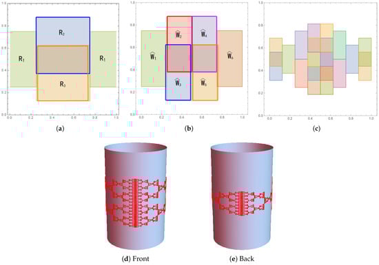
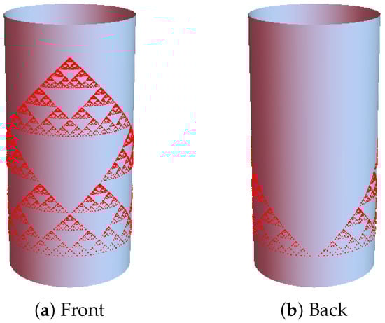
Let K be the associated attractor (see Figure 1). Then

$${dim}_{\mathrm{H}}\left(K\right)={\displaystyle \frac{log3}{log2}}=1.58496\dots$$

Figure 1. Figures for Example 1 with $r=\pi /4$. (a–c) are drawn on ${\mathbb{R}}^2$ and shrunk by $2\pi$. (a) The first iteration of $E_0$ under ${\left\{R_t\right\}}_{t=1}^3$, where $R_1\left(E_0\right)$ consists of the left and right rectangles, $R_2\left(E_0\right)$ is the top square, and $R_3\left(E_0\right)$ is the bottom square. (b) Vertices of the GIFS associated with ${\left\{R_t\right\}}_{t=1}^3$. (c) The first iteration of the vertices under the GIFS. (d,e) The attractor of ${\left\{R_t\right\}}_{t=1}^3$.

Proof of Example 1.

For any $t\in \{1,2,3\}$, by the definition of $R_t$, we have $H_t^1=H_t:=\{(-1,0,z):z\in [0,2\pi ]\}$. Let $r_t:=R_t{|}_{H_t}$ and $r_t\left(H_t\right)={\bigcup }_{l=1}^2{h}_t^{l,1}\left(H_t^1\right)$. Then for any $\mathit{x}\in H_t^1$,

$$\begin{array}{cccc}\hfill & h_1^{1,1}\left(\mathit{x}\right)=(0,1,z/2+\pi /2),\hfill & \hfill & h_1^{2,1}\left(\mathit{x}\right)=(0,-1,z/2+\pi /2),\hfill \\ \hfill & h_2^{1,1}\left(\mathit{x}\right)=(0,-1,z/2+\pi -r),\hfill & \hfill & h_2^{2,1}\left(\mathit{x}\right)=(0,1,z/2+\pi -r),\hfill \\ \hfill & h_3^{1,1}\left(\mathit{x}\right)=(0,-1,z/2+r),\hfill & \hfill & h_3^{2,1}\left(\mathit{x}\right)=(0,1,z/2+r).\hfill \end{array}$$

For any $t\in \{1,2,3\}$, let

$$\begin{array}{cc}\hfill & J_t^1:=\left\{(cos\theta ,sin\theta ,z):\theta \in (-\pi ,0],z\in [0,2\pi ]\right\}\mathrm{and}\hfill \\ \hfill & J_t^2:=\left\{(cos\theta ,sin\theta ,z):\theta \in (0,\pi ),z\in [0,2\pi ]\right\}.\hfill \end{array}$$

Then $E_0\setminus H_t={\bigcup }_{i=1}^2{J}_t^i$. Let ${\tilde{r}}_t:=R_t{|}_{E_0\setminus H_t}$ and ${\tilde{r}}_t(E_0\setminus H_t)={\bigcup }_{i=1}^2{h}_t^{0,i}\left(J_t^i\right)$. Then for any $\mathit{x}\in J_t^i$, where $i\in \{1,2\}$,

$$\begin{array}{cc}\hfill & h_1^{0,i}\left(\mathit{x}\right)=(-cos(\theta /2),-sin(\theta /2),z/2+\pi /2),\hfill \\ \hfill & h_2^{0,i}\left(\mathit{x}\right)=(cos(\theta /2),sin(\theta /2),z/2+\pi -r),\hfill \\ \hfill & h_3^{0,i}\left(\mathit{x}\right)=(cos(\theta /2),sin(\theta /2),z/2+r).\hfill \end{array}$$

Hence, for any $t\in \{1,2,3\}$, $h_t^{l,1}$ are contractions, where $l\in \{1,2\}$, and $h_t^{0,i}$ are contractions, where $i\in \{1,2\}$. Moreover, for $t=1$, we have

$$\begin{array}{c}\hfill \overline{h_t^{1,1}\left(H_t\right)}\subseteq \overline{J_t^2},\overline{h_t^{2,1}\left(H_t\right)}\subseteq \overline{J_t^1},\overline{h_t^{0,1}\left(J_t^1\right)}\subseteq \overline{J_t^2},\overline{h_t^{0,2}\left(J_t^2\right)}\subseteq \overline{J_t^1};\end{array}$$

for any $t\in \{2,3\}$, we have

$$\begin{array}{c}\hfill \overline{h_t^{1,1}\left(H_t\right)}\subseteq \overline{J_t^1},\overline{h_t^{2,1}\left(H_t\right)}\subseteq \overline{J_t^2},\overline{h_t^{0,i}\left(J_t^i\right)}\subseteq \overline{J_t^i},\mathrm{where}i\in \{1,2\}.\end{array}$$

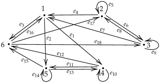
Hence, ${\left\{R_t\right\}}_{t=1}^3$ satisfies the conditions of Theorem 6. By Theorem 6 and Proposition 5, we can find a minimal simplified GIFS $\widehat{G}=(\widehat{V},\widehat{E})$ with $\widehat{V}=\{1,\dots ,6\}$ and $\widehat{E}=\{e_1,\dots ,e_{18}\}$ (see Figure 2).

Figure 2. The GIFS associated with ${\left\{R_t\right\}}_{t=1}^3$ in Example 1.

The invariant family ${\left\{{\widehat{W}}_i\right\}}_{i=1}^6$ is defined as

$$\begin{array}{cc}\hfill & {\widehat{W}}_1:=\{(cos\theta ,sin\theta ,z):\theta \in [-\pi ,-\pi /2],z\in [\pi /2,3\pi /2]\},\hfill \\ \hfill & {\widehat{W}}_2:=\{(cos\theta ,sin\theta ,z):\theta \in [-\pi /2,0],z\in [\pi -r,2\pi -r]\},\hfill \\ \hfill & {\widehat{W}}_3:=\{(cos\theta ,sin\theta ,z):\theta \in [-\pi /2,0],z\in [r,\pi +r]\},\hfill \\ \hfill & {\widehat{W}}_4:=\{(cos\theta ,sin\theta ,z):\theta \in [0,\pi /2],z\in [\pi -r,2\pi -r]\},\hfill \\ \hfill & {\widehat{W}}_5:=\{(cos\theta ,sin\theta ,z):\theta \in [0,\pi /2],z\in [r,\pi +r]\},\hfill \\ \hfill & {\widehat{W}}_6:=\{(cos\theta ,sin\theta ,z):\theta \in [\pi /2,\pi ],z\in [\pi /2,3\pi /2]\},\hfill \end{array}$$

while ${\widehat{E}}^{i,j}$, $i,j\in \{1,\dots ,6\}$, and the associated similitudes ${\left\{f_e\right\}}_{e\in \widehat{E}}$ are defined as

$$\begin{array}{ccccccc}& e_1\in {\widehat{E}}^{1,4},\hfill & \hfill e_2\in {\widehat{E}}^{1,5},& e_3\in {\widehat{E}}^{1,6},\hfill & \hfill e_4\in {\widehat{E}}^{2,1},& e_5\in {\widehat{E}}^{2,2},\hfill & \hfill e_6\in {\widehat{E}}^{2,3},\\ & e_7\in {\widehat{E}}^{3,1},\hfill & \hfill e_8\in {\widehat{E}}^{3,2},& e_9\in {\widehat{E}}^{3,3},\hfill & \hfill e_{10}\in {\widehat{E}}^{4,4},& e_{11}\in {\widehat{E}}^{4,5},\hfill & \hfill e_{12}\in {\widehat{E}}^{4,6},\\ & e_{13}\in {\widehat{E}}^{5,4},\hfill & \hfill e_{14}\in {\widehat{E}}^{5,5},& e_{15}\in {\widehat{E}}^{5,6},\hfill & \hfill e_{16}\in {\widehat{E}}^{6,1},& e_{17}\in {\widehat{E}}^{6,2},\hfill & \hfill e_{18}\in {\widehat{E}}^{6,3},\end{array}$$

and

$$\begin{array}{cc}\hfill & f_{e_1}:={\tilde{h}}_1^{0,2}{|}_{{\widehat{W}}_4},f_{e_2}:={\tilde{h}}_1^{0,2}{|}_{{\widehat{W}}_5},f_{e_3}:={\tilde{h}}_1^{0,2}{|}_{{\widehat{W}}_6},f_{e_4}:={\tilde{h}}_2^{0,1}{{|}_{{\widehat{W}}_1},f_{e_5}:={\tilde{h}}_2^{0,1}|}_{{\widehat{W}}_2},\hfill \\ & f_{e_6}:={\tilde{h}}_2^{0,1}{|}_{{\widehat{W}}_3},f_{e_7}:={\tilde{h}}_3^{0,1}{|}_{{\widehat{W}}_1},f_{e_8}:={\tilde{h}}_3^{0,1}{|}_{{\widehat{W}}_2},f_{e_9}:={\tilde{h}}_3^{0,1}{{|}_{{\widehat{W}}_3},f_{e_{10}}:={\tilde{h}}_2^{0,2}|}_{{\widehat{W}}_4},\hfill \\ \hfill & f_{e_{11}}:={\tilde{h}}_2^{0,2}{|}_{{\widehat{W}}_5},f_{e_{12}}:={\tilde{h}}_2^{0,2}{|}_{{\widehat{W}}_6},f_{e_{13}}:={\tilde{h}}_3^{0,2}{|}_{{\widehat{W}}_4},f_{e_{14}}:={\tilde{h}}_3^{0,2}{{|}_{{\widehat{W}}_5},f_{e_{15}}:={\tilde{h}}_3^{0,2}|}_{{\widehat{W}}_6},\hfill \\ \hfill & f_{e_{16}}:={\tilde{h}}_1^{0,1}{|}_{{\widehat{W}}_1},f_{e_{17}}:={\tilde{h}}_1^{0,1}{{|}_{{\widehat{W}}_2},f_{e_{18}}:={\tilde{h}}_1^{0,1}|}_{{\widehat{W}}_3},\hfill \end{array}$$

where ${\tilde{h}}_t^{l,i}$ and ${\tilde{h}}_t^{0,i}$ are defined as in (6) and (12), respectively.

Note that $\widehat{G}$ is strongly connected. Let

$$\begin{array}{cc}\hfill {\underline{W}}_1& :=\left\{\right(cos\theta ,sin\theta ,z):\theta \in (-\pi ,-\pi /2),z\in (\pi /2+r,3\pi /2-r\left)\right\},\hfill \\ \hfill {\underline{W}}_2& :=\left\{\right(cos\theta ,sin\theta ,z):\theta \in (-\pi /2,0),z\in (3\pi /2-2r,2\pi -2r\left)\right\},\hfill \\ \hfill {\underline{W}}_3& :=\left\{\right(cos\theta ,sin\theta ,z):\theta \in (-\pi /2,0),z\in (2r,2r+\pi /2\left)\right\},\hfill \\ \hfill {\underline{W}}_4& :=\left\{\right(cos\theta ,sin\theta ,z):\theta \in (0,\pi /2),z\in (3\pi /2-2r,2\pi -2r\left)\right\},\hfill \\ \hfill {\underline{W}}_5& :=\left\{\right(cos\theta ,sin\theta ,z):\theta \in (0,\pi /2),z\in (2r,2r+\pi /2\left)\right\},\hfill \\ \hfill {\underline{W}}_6& :=\left\{\right(cos\theta ,sin\theta ,z):\theta \in (\pi /2,\pi ),z\in (\pi /2+r,3\pi /2-r\left)\right\}.\hfill \end{array}$$

Let

$${\tilde{K}}_i=\bigcup _{j=1}^6\bigcup _{e\in {\widehat{E}}^{i,j}}{f}_e\left({\tilde{K}}_j\right).$$

Then for $i\in \{1,\dots ,6\}$, $U_i:={\underline{W}}_i\setminus {\tilde{K}}_i$ is an open set. For all $i\in \{1,\dots ,6\}$, ${\left\{f_e\right\}}_{e\in \widehat{E}}$ satisfies

$$\begin{array}{c}\hfill \bigcup _{e\in {\widehat{E}}^{i,j}}{f}_e\left(U_j\right)\subseteq U_i\mathrm{and}{f}_{e_1}\left(U_{j_1}\right)\bigcap f_{e_2}\left(U_{j_2}\right)=Ø,\mathrm{for}{e}_1\in {\widehat{E}}^{i,j_1}\mathrm{and}{e}_2\in {\widehat{E}}^{i,j_2}.\end{array}$$

Hence, $\widehat{G}$ satisfies (GOSC). The weighted incidence matrix associated with $\widehat{G}$ is

$$A_{\alpha }={\left({\displaystyle \frac{1}{2}}\right)}^{\alpha }\left[\begin{array}{c}\begin{array}{cccccc}0& 0& 0& 1& 1& 1\\ 1& 1& 1& 0& 0& 0\\ 1& 1& 1& 0& 0& 0\\ 0& 0& 0& 1& 1& 1\\ 0& 0& 0& 1& 1& 1\\ 1& 1& 1& 0& 0& 0\end{array}\end{array}\right].$$

The spectral radius of ${\widehat{A}}_{\alpha }$ is $3{(1/2)}^{\alpha }$. Therefore,

$${dim}_{\mathrm{H}}\left(K\right)={\displaystyle \frac{log3}{log2}}=1.58496\dots$$

□

6. Hausdorff Dimension of Graph Self-Similar Sets with Overlaps

In this section, we study IRSs with overlaps (see Definition 10). We give the definition of the graph finite type condition (GFTC) and prove Theorems 4–5. Moreover, we illustrate our method for computing the Hausdorff dimension of the associated attractors using several examples.

6.1. Graph Finite Type Condition

For detailed definitions of the notation in this section, especially the definition of a sequence of nested index sets, the reduced graph, and the neighborhood of a vertex in the reduced graph, we refer the reader to [6,14]. Here we only give a very brief summary. Let $G=(V,E)$ be a GIFS as described in Section 4. Let ${\left\{{\mathcal{M}}_k\right\}}_{k=0}^{\infty }$ be a sequence of nested index sets (see [14]), where ${\mathcal{M}}_k\subseteq E^{*}$ and $E^{*}$ is defined as in Section 4. For $i,j\in \{1,\dots ,m\}$, let

$${\mathcal{M}}_k^{i,j}:={\mathcal{M}}_k\bigcap \left(\bigcup _{q\ge 1}{E}_q^{i,j}\right)=\left\{\mathbf{e}=(e_1,\dots ,e_q)\in {\mathcal{M}}_k:\mathbf{e}\in E_q^{i,j}\mathrm{for}\mathrm{some}q\ge 1\right\}.$$

Then ${\mathcal{M}}_k={\bigcup }_{i,j=1}^m{\mathcal{M}}_k^{i,j}$. For $\mathbf{e}\in {\mathcal{M}}_k^{i,j}$, let $f_{\mathbf{e}}:=f_{e_1}\circ \cdots \circ f_{e_q}$, where each $f_{e_i}$ is a contraction on G. Define

$${\mathcal{V}}_k^{i,j}:=\left\{(f_{\mathbf{e}},i,j,k),\mathbf{e}\in {\mathcal{M}}_k^{i,j}\right\}\mathrm{for}i,j=1,\dots ,m,\mathrm{and}{\mathcal{V}}_k:=\bigcup _{i,j=1}^m{\mathcal{V}}_k^{i,j}\mathrm{for}k\ge 1.$$

For $\mathbf{e}\in {\mathcal{M}}_k^{i,j}$, we call $(f_{\mathbf{e}},i,j,k)$ a vertex and $\mathcal{V}:={\bigcup }_{k\ge 0}{\mathcal{V}}_k$ the vertex set. Define a graph $\mathcal{G}:=(\mathcal{V},\mathcal{E})$, where $\mathcal{E}$ is the set of all directed edges of $\mathcal{V}$. Let ${\mathcal{G}}_{\mathcal{R}}=({\mathcal{V}}_{\mathcal{R}},{\mathcal{E}}_{\mathcal{R}})$ be the reduced graph of $\mathcal{G}$ (see, e.g., [14] for the construction of ${\mathcal{G}}_{\mathcal{R}}$). Let $\widehat{\mathcal{G}}:=(\widehat{\mathcal{V}},\widehat{\mathcal{E}})$ be a minimal simplified GIFS associated with $\mathcal{G}$. We can use a similar method to construct a corresponding reduced GIFS ${\widehat{\mathcal{G}}}_{\mathcal{R}}:=({\widehat{\mathcal{V}}}_{\mathcal{R}},{\widehat{\mathcal{E}}}_{\mathcal{R}})$. Two vertices $\mathbf{v}\in {\mathcal{V}}_k$ and ${\mathbf{v}}^{\prime }\in {\mathcal{V}}_{k^{\prime }}$ are equivalent, denoted $\mathbf{v}\sim {\mathbf{v}}^{\prime }$, if $\#\mathcal{N}\left(\mathbf{v}\right)=\#\mathcal{N}\left({\mathbf{v}}^{\prime }\right)$, where $\mathcal{N}\left(\mathbf{v}\right)$ is a neighborhood of $\mathbf{v}$ (see, e.g., [14]), and $\tau =f_{{\mathbf{v}}^{\prime }}\circ f_{\mathbf{v}}^{-1}:M\to M$ induces a bijection $g_{\tau }:\mathcal{N}\left(\mathbf{v}\right)\to \mathcal{N}\left({\mathbf{v}}^{\prime }\right)$, which is defined as

$$\begin{array}{c}\hfill g_{\tau }(f_{\mathbf{u}},i,j,k)=(\tau \circ f_{\mathbf{u}},i^{\prime },j^{\prime },k^{\prime }),\end{array}$$

(29)

and satisfies the following conditions:

(a)

In (29), $j=j^{\prime }$.

(b)

For $\mathbf{u}\in \mathcal{N}\left(\mathbf{v}\right)$ and ${\mathbf{u}}^{\prime }\in \mathcal{N}\left({\mathbf{v}}^{\prime }\right)$ satisfying $g_{\tau }\left(\mathbf{u}\right)={\mathbf{u}}^{\prime }$, and for any integer $l\ge 1$, a directed path $\mathbf{e}\in E^{*}$ satisfies $(f_{\mathbf{u}}\circ f_{\mathbf{e}},k+l)\in {\mathcal{V}}_{k+l}$ if and only if it satisfies $(f_{{\mathbf{u}}^{\prime }}\circ f_{\mathbf{e}},k^{\prime }+l)\in {\mathcal{V}}_{k^{\prime }+l}$.

Let $\left[\mathbf{v}\right]$ denote the equivalence class of $\mathbf{v}$. We call $\left[\mathbf{v}\right]$ the neighborhood type of $\mathbf{v}$ (with respect to $\mathbf{U}$), where $\mathbf{U}:={\left\{U_i\right\}}_{i=1}^m$ is an invariant family under G.

Definition 12. 

Let X be a complete metric space. Let $G=(V,E)$ be a GIFS of contractions ${\left\{f_e\right\}}_{e\in E}$ on X, where $V=\{1,\dots ,m\}$. If there exists an invariant family of nonempty bounded open sets $\mathbf{U}={\left\{U_i\right\}}_{i=1}^m$ with respect to some sequence of nested index sets ${\left\{{\mathcal{M}}_k\right\}}_{k=0}^{\infty }$ such that $\#\mathcal{V}{/}_{\sim }:=\{{\left[\mathbf{v}\right]}_{\mathbf{U}},\mathbf{v}\in \mathcal{V}\}$ is a finite set, where ∼ is an equivalence relation on $\mathcal{V}$, then we say that $G=(V,E)$ satisfies the graph finite type condition (GFTC). We say that $\mathbf{U}$ is a finite type condition family.

Definition 13. 

Let X be a complete metric space. Let ${\left\{R_t\right\}}_{t=1}^N$ be an IRS on a nonempty compact subset of X. Assume that there exists a GIFS G associated with ${\left\{R_t\right\}}_{t=1}^N$, and assume that G consists of contractions. If G satisfies (GFTC), then we say that${\left\{R_t\right\}}_{t=1}^N$satisfies (GFTC) with respect to G.

The following theorem is a direct generalization of Theorem 2.7 in [26]; it provides a sufficient condition for a GIFS to satisfy the finite type condition. Recall that an algebraic integer $\beta >1$ is called a Pisot number if all of its algebraic conjugates are in modulus strictly less than one.

Theorem 8. 

Let M be a complete smooth n-dimensional Riemannian manifold that is locally Euclidean. Let $G=(V,E)$ be a GIFS of contractive similitudes ${\left\{f_e\right\}}_{e\in E}$ on M. Let ${\left\{W_i\right\}}_{i=1}^m$ be an invariant family of nonempty compact sets, and let $\mathbf{U}:={\left\{U_i\right\}}_{i=1}^m$ be an invariant family of nonempty bounded open sets with ${\overline{U}}_i=W_i$, $i=1,\dots ,m$. For each similitude $f_e$, $e\in E$, assume that there exists an isometry

$$g_i:U_i\to U_i^{\prime }\subseteq {\mathbb{R}}^n$$

such that for any $e^{\prime }\in E^{\prime }$, $f_{e^{\prime }}^{\prime }:=g_i\circ f_e\circ g_i^{-1}$ is contractive similitude of the form

$$f_{e^{\prime }}^{\prime }\left(x\right)={\beta }^{-n_{e^{\prime }}}{R}_{e^{\prime }}\left(x\right)+b_{e^{\prime }},$$

where $E^{\prime }$ is a set of directed edges, $\beta >1$ is a Pisot number, $n_{e^{\prime }}$ is a positive integer, $R_{e^{\prime }}$ is an orthogonal transformation, and $b_{e^{\prime }}\in {\mathbb{R}}^n$. Assume that ${\left\{R_{e^{\prime }}\right\}}_{e^{\prime }\in E^{\prime }}$ generates a finite group H and

$$H\left\{b_{e^{\prime }}\right|e^{\prime }\in E^{\prime }\}\subseteq r_1\mathbb{Z}\left[\beta \right]\times \cdots \times r_n\mathbb{Z}\left[\beta \right]$$

for some $r_1,\dots ,r_n\in \mathbb{R}$. Then G is of finite type, and $\mathbf{U}$ is a finite type condition family of G.

Proof. 

By the assumptions, we let $V^{\prime }:=\{1,\dots ,m\}$ be a set of vertices. Then $G^{\prime }:=(V^{\prime },E^{\prime })$ is a GIFS of contractive similitudes ${\left\{f_{e^{\prime }}^{\prime }\right\}}_{e^{\prime }\in E^{\prime }}$ on ${\mathbb{R}}^n$, and ${\mathbf{U}}^{\prime }:={\left\{U_i^{\prime }\right\}}_{i=1}^m$ is an invariant family of nonempty bounded open sets for $G^{\prime }$. By the results of Theorem 2.7 in [26], we have $G^{\prime }$ is of finite type and ${\mathbf{U}}^{\prime }$ is a finite type condition family for $G^{\prime }$. Let ${\mathbf{v}}^{\prime }:=(f_{{\mathbf{e}}^{\prime }}^{\prime },i,j,k)\in {\mathcal{V}}^{\prime }$ be a vertex, ${\mathbf{e}}^{\prime }\in {\tilde{\mathcal{M}}}_k^{i,j}$, $1\le i,j\le m$, $k\ge 1$, and ${\tilde{\mathcal{M}}}_k^{i,j}\subseteq {\left(E^{\prime }\right)}^{*}$ is a sequence of nested index sets. Then $\{{\left[{\mathbf{v}}^{\prime }\right]}_{{\mathbf{U}}^{\prime }},{\mathbf{v}}^{\prime }\in {\mathcal{V}}^{\prime }\}$ is a finite set. Let $\mathbf{v}:=(f_{\mathbf{e}},i,j,k)\in \mathcal{V}$, where $\mathbf{e}\in {\mathcal{M}}_k^{i,j}$, $1\le i,j\le m$, and ${\mathcal{M}}_k^{i,j}\subseteq E^{*}$ is a sequence of nested index sets. It follows from the definition of $f_{{\mathbf{e}}^{\prime }}^{\prime }$ that $\{{\left[\mathbf{v}\right]}_{\mathbf{U}},\mathbf{v}\in \mathcal{V}\}=\{{\left[{\mathbf{v}}^{\prime }\right]}_{{\mathbf{U}}^{\prime }},{\mathbf{v}}^{\prime }\in {\mathcal{V}}^{\prime }\}$ is a finite set. This proves the proposition.  □

We let ${\mathcal{T}}_1,\dots ,{\mathcal{T}}_m$ denote the collection of all distinct neighborhood types, with $\left[{\mathbf{v}}_{\mathrm{root}}^i\right]$, $i=1,\dots ,m$, being the neighborhood types of the root vertices. As in [14], for each $\alpha \ge 0$, we define a weighted incidence matrix $A_{\alpha }={\left(A_{\alpha }(i,j)\right)}_{i,j=1}^m$ as follows. Fix i ($1\le i\le m$) and a vertex $\mathbf{v}\in {\mathcal{V}}_{\mathcal{R}}$ such that $\left[\mathbf{v}\right]={\mathcal{T}}_i$, let ${\mathbf{u}}_1,\dots ,{\mathbf{u}}_m$ be the offspring of $\mathbf{v}$ in ${\mathcal{V}}_{\mathcal{R}}$, and let ${\mathbf{k}}_l$, $1\le l\le m$, be the unique edge in ${\mathcal{G}}_{\mathcal{R}}$ connecting $\mathbf{v}$ to ${\mathbf{u}}_l$. Then we define

$$\begin{array}{c}\hfill A_{\alpha }(i,j):=\sum \{{\rho }_{{\mathbf{k}}_l}^{\alpha }:\mathbf{v}\stackrel{{\mathbf{k}}_l}{⟶}{\mathbf{u}}_l,\left[{\mathbf{u}}_l\right]={\mathcal{T}}_j\}.\end{array}$$

(30)

Now we are ready to prove Theorems 4 and 5, which are stated in Section 2.

Proof f Theorem 4.

By Proposition 3, we know that G and ${\left\{R_t\right\}}_{t=1}^N$ have the same attractor. The proof follows by using the results of Theorem 1.6 in [6]; we omit the details.  □

Proof of Theorem 5.

Combining Proposition 3 and Definition 6, we know that the attractor of G is equal to that of $\widehat{G}$. The proof follows by using the results of Theorem 4.  □

6.2. Examples

In this subsection, we give three examples of IRSs with overlaps that satisfy (GFTC).

Example 2. 

Let ${\mathcal{C}}^2=\left\{(cos\theta ,sin\theta ,z):\theta \in [-\pi ,\pi ],z\in [0,2\pi ]\right\}$ be a cylindrical surface. Let $E_0:={\mathcal{C}}^2$. For $r\in [0,\pi /2)$, we let $\mathit{x}:=(cos\theta ,sin\theta ,z)$ and let ${\left\{R_t\right\}}_{t=1}^4$ be an IRS on $E_0$ defined as

$$\begin{array}{cc}\hfill & R_1\left(\mathit{x}\right):=\left\{\begin{array}{cc}(-cos(\theta /2),-sin(\theta /2),z/2+\pi /2)\hfill & \mathit{x}\in E_0\setminus \{(-1,0,z):z\in [0,2\pi ]\},\hfill \\ \left\{\right(0,-1,z/2+\pi /2),(0,1,z/2+\pi /2\left)\right\}\hfill & \mathit{x}\in \left\{\right(-1,0,z):z\in [0,2\pi \left]\right\};\hfill \end{array}\right.\hfill \\ \hfill & R_2\left(\mathit{x}\right):=\left\{\begin{array}{cc}(cos(\theta /2),sin(\theta /2),z/2+\pi -r)\hfill & \mathit{x}\in E_0\setminus \{(-1,0,z):z\in [0,2\pi ]\},\hfill \\ \left\{\right(0,1,z/2+\pi -r),(0,-1,z/2+\pi -r\left)\right\}\hfill & \mathit{x}\in \left\{\right(-1,0,z):z\in [0,2\pi \left]\right\};\hfill \end{array}\right.\hfill \\ \hfill & R_3\left(\mathit{x}\right):=\left\{\begin{array}{cc}(cos(\theta /2),sin(\theta /2),z/2+\pi /2)\hfill & \mathit{x}\in E_0\setminus \{(-1,0,z):z\in [0,2\pi ]\},\hfill \\ \left\{\right(0,1,z/2+\pi /2),(0,-1,z/2+\pi /2\left)\right\}\hfill & \mathit{x}\in \left\{\right(-1,0,z):z\in [0,2\pi \left]\right\};\hfill \end{array}\right.\hfill \\ \hfill & R_4\left(\mathit{x}\right):=\left\{\begin{array}{cc}(cos(\theta /2),sin(\theta /2),z/2+r)\hfill & \mathit{x}\in E_0\setminus \{(-1,0,z):z\in [0,2\pi ]\},\hfill \\ \left\{\right(0,1,z/2+r),(0,-1,z/2+r\left)\right\}\hfill & \mathit{x}\in \left\{\right(-1,0,z):z\in [0,2\pi \left]\right\}.\hfill \end{array}\right.\hfill \end{array}$$

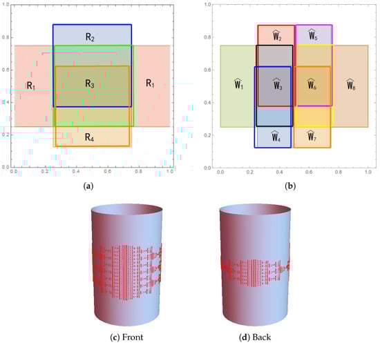
Let K be the associated attractor (see Figure 3). Then

$${dim}_{\mathrm{H}}\left(K\right)={\displaystyle \frac{log(2+\sqrt{2})}{log2}}=1.77155\dots$$

Figure 3. Figures for Example 2 with $r=\pi /4$. (a,b) are drawn on ${\mathbb{R}}^2$ and shrunk by $2\pi$. (a) The first iteration of $E_0$ under ${\left\{R_t\right\}}_{t=1}^4$, where $R_1\left(E_0\right)$ consists of the left and right rectangles, $R_2\left(E_0\right)$ is the top square, $R_3\left(E_0\right)$ is the middle square, and $R_4\left(E_0\right)$ is the bottom square. (b) Vertices of the GIFS associated with ${\left\{R_t\right\}}_{t=1}^4$. (c,d) The attractor of ${\left\{R_t\right\}}_{t=1}^4$.

Proof of Example 2.

For any $t\in \{1,\dots ,4\}$, by the definition of $R_t$, we have $H_t^1=H_t:=\{(-1,0,z):z\in [0,2\pi ]\}$. Let $r_t:=R_t{|}_{H_t}$ and $r_t\left(H_t\right)={\bigcup }_{l=1}^2{h}_t^{l,1}\left(H_t^1\right)$. Then for any $\mathit{x}\in H_t^1$,

$$\begin{array}{cccc}\hfill & h_1^{1,1}\left(\mathit{x}\right)=(0,1,z/2+\pi /2),\hfill & \hfill & h_1^{2,1}\left(\mathit{x}\right)=(0,-1,z/2+\pi /2),\hfill \\ \hfill & h_2^{1,1}\left(\mathit{x}\right)=(0,-1,z/2+\pi -r),\hfill & \hfill & h_2^{2,1}\left(\mathit{x}\right)=(0,1,z/2+\pi -r),\hfill \\ \hfill & h_3^{1,1}\left(\mathit{x}\right)=(0,-1,z/2+\pi /2),\hfill & \hfill & h_3^{2,1}\left(\mathit{x}\right)=(0,1,z/2+\pi /2),\hfill \\ \hfill & h_4^{1,1}\left(\mathit{x}\right)=(0,-1,z/2+r),\hfill & \hfill & h_4^{2,1}\left(\mathit{x}\right)=(0,1,z/2+r).\hfill \end{array}$$

For any $t\in \{1,\dots ,4\}$, by the definition of $R_t$, we have

$$\begin{array}{cc}\hfill & J_t^1:=\left\{(cos\theta ,sin\theta ,z):\theta \in (-\pi ,0],z\in [0,2\pi ]\right\}and\hfill \\ \hfill & J_t^2:=\left\{(cos\theta ,sin\theta ,z):\theta \in (0,\pi ),z\in [0,2\pi ]\right\}.\hfill \end{array}$$

Hence, $E_0\setminus H_t={\bigcup }_{i=1}^2{J}_t^i$. Let ${\tilde{r}}_t:=R_t{|}_{E_0\setminus H_t}$ and ${\tilde{r}}_t(E_0\setminus H_t)={\bigcup }_{i=1}^2{h}_t^{0,i}\left(J_t^i\right)$. Then for any $\mathit{x}\in J_t^i$, where $i\in \{1,2\}$,

$$\begin{array}{cc}\hfill & h_1^{0,i}\left(\mathit{x}\right)=(-cos(\theta /2),-sin(\theta /2),z/2+\pi /2),\hfill \\ \hfill & h_2^{0,i}\left(\mathit{x}\right)=(cos(\theta /2),sin(\theta /2),z/2+\pi -r),\hfill \\ \hfill & h_3^{0,i}\left(\mathit{x}\right)=(cos(\theta /2),sin(\theta /2),z/2+\pi /2),\hfill \\ \hfill & h_4^{0,i}\left(\mathit{x}\right)=(cos(\theta /2),sin(\theta /2),z/2+r).\hfill \end{array}$$

Hence, for any $t\in \{1,\dots ,4\}$ and $l\in \{1,2\}$, $h_t^{l,1}$ are contractions, and for any $i\in \{1,2\}$, $h_t^{0,i}$ are contractions. Moreover, for $t=1$, we have

$$\begin{array}{c}\hfill \overline{h_t^{1,1}\left(H_t\right)}\subseteq \overline{J_t^2},\overline{h_t^{2,1}\left(H_t\right)}\subseteq \overline{J_t^1},\overline{h_t^{0,1}\left(J_t^1\right)}\subseteq \overline{J_t^2},\overline{h_t^{0,2}\left(J_t^2\right)}\subseteq \overline{J_t^1};\end{array}$$

for any $t\in \{2,3,4\}$,

$$\begin{array}{c}\hfill \overline{h_t^{1,1}\left(H_t\right)}\subseteq \overline{J_t^1},\overline{h_t^{2,1}\left(H_t\right)}\subseteq \overline{J_t^2},\overline{h_t^{0,i}\left(J_t^i\right)}\subseteq \overline{J_t^i},\mathrm{where}i\in \{1,2\}.\end{array}$$

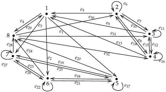
Hence, ${\left\{R_t\right\}}_{t=1}^4$ satisfies the conditions of Theorem 6. By Theorem 6 and Proposition 5, we can find a minimal simplified GIFS $\widehat{G}=(\widehat{V},\widehat{E})$ with $\widehat{V}=\{1,\dots ,8\}$ and $\widehat{E}=\{e_1,\dots ,e_{32}\}$ (see Figure 4).

Figure 4. The GIFS associated with ${\left\{R_t\right\}}_{t=1}^4$ in Example 2.

The invariant family ${\left\{{\widehat{W}}_i\right\}}_{i=1}^8$, the set of edges ${\widehat{E}}^{i,j}$ and the associated similitudes ${\left\{f_e\right\}}_{e\in \widehat{E}}$ are defined as

$$\begin{array}{cc}\hfill {\widehat{W}}_1& :=\left\{\right(cos\theta ,sin\theta ,z):\theta \in [-\pi ,-\pi /2],z\in [\pi /2,3\pi /2\left]\right\},\hfill \\ \hfill {\widehat{W}}_2& :=\left\{\right(cos\theta ,sin\theta ,z):\theta \in [-\pi /2,0],z\in [\pi -r,2\pi -r\left]\right\},\hfill \\ \hfill {\widehat{W}}_3& :=\left\{\right(cos\theta ,sin\theta ,z):\theta \in [-\pi /2,0],z\in [\pi /2,3\pi /2\left]\right\},\hfill \\ \hfill {\widehat{W}}_4& :=\left\{\right(cos\theta ,sin\theta ,z):\theta \in [-\pi /2,0],z\in [r,\pi +r\left]\right\}\hfill \\ \hfill {\widehat{W}}_5& :=\left\{\right(cos\theta ,sin\theta ,z):\theta \in [0,\pi /2],z\in [\pi -r,2\pi -r\left]\right\},\hfill \\ \hfill {\widehat{W}}_6& :=\left\{\right(cos\theta ,sin\theta ,z):\theta \in [0,\pi /2],z\in [\pi /2,3\pi /2\left]\right\},\hfill \\ \hfill {\widehat{W}}_7& :=\left\{\right(cos\theta ,sin\theta ,z):\theta \in [0,\pi /2],z\in [r,\pi +r\left]\right\},\hfill \\ \hfill {\widehat{W}}_8& :=\left\{\right(cos\theta ,sin\theta ,z):\theta \in [\pi /2,\pi ],z\in [\pi /2,3\pi /2\left]\right\},\hfill \end{array}$$

$$\begin{array}{ccccccc}& e_1\in {\widehat{E}}^{1,5},\hfill & \hfill e_2\in {\widehat{E}}^{1,6},& e_3\in {\widehat{E}}^{1,7},\hfill & \hfill e_4\in {\widehat{E}}^{1,8},& e_5\in {\widehat{E}}^{2,1},\hfill & \hfill e_6\in {\widehat{E}}^{2,2},\\ & e_7\in {\widehat{E}}^{2,3},\hfill & \hfill e_8\in {\widehat{E}}^{2,4},& e_9\in {\widehat{E}}^{3,1},\hfill & \hfill e_{10}\in {\widehat{E}}^{3,2},& e_{11}\in {\widehat{E}}^{3,3},\hfill & \hfill e_{12}\in {\widehat{E}}^{3,4},\\ & e_{13}\in {\widehat{E}}^{4,1},\hfill & \hfill e_{14}\in {\widehat{E}}^{4,2},& e_{15}\in {\widehat{E}}^{4,3},\hfill & \hfill e_{16}\in {\widehat{E}}^{4,4},& e_{17}\in {\widehat{E}}^{5,5},\hfill & \hfill e_{18}\in {\widehat{E}}^{5,6},\\ & e_{19}\in {\widehat{E}}^{5,7},\hfill & \hfill e_{20}\in {\widehat{E}}^{5,8},& e_{21}\in {\widehat{E}}^{6,5},\hfill & \hfill e_{22}\in {\widehat{E}}^{6,6},& e_{23}\in {\widehat{E}}^{6,7},\hfill & \hfill e_{24}\in {\widehat{E}}^{6,8},\\ & e_{25}\in {\widehat{E}}^{7,5},\hfill & \hfill e_{26}\in {\widehat{E}}^{7,6},& e_{27}\in {\widehat{E}}^{7,7},\hfill & \hfill e_{28}\in {\widehat{E}}^{7,8},& e_{29}\in {\widehat{E}}^{8,1},\hfill & \hfill e_{30}\in {\widehat{E}}^{8,2},\\ & e_{31}\in {\widehat{E}}^{8,3},\hfill & \hfill e_{32}\in {\widehat{E}}^{8,4},& \hfill & \hfill & \hfill \end{array}$$

and

$$\begin{array}{cccccc}& f_{e_1}:={\tilde{h}}_1^{0,2}{|}_{{\widehat{W}}_5},\hfill & \hfill f_{e_2}:={\tilde{h}}_1^{0,2}{|}_{{\widehat{W}}_6},& f_{e_3}:={\tilde{h}}_1^{0,2}{|}_{{\widehat{W}}_7},\hfill & \hfill f_{e_4}:={\tilde{h}}_1^{0,2}{|}_{{\widehat{W}}_8},& f_{e_5}:={\tilde{h}}_2^{0,1}{|}_{{\widehat{W}}_1},\hfill \\ & f_{e_6}:={\tilde{h}}_2^{0,1}{|}_{{\widehat{W}}_2},\hfill & \hfill f_{e_7}:={\tilde{h}}_2^{0,1}{|}_{{\widehat{W}}_3},& f_{e_8}:={\tilde{h}}_2^{0,1}{|}_{{\widehat{W}}_4},\hfill & \hfill f_{e_9}:={\tilde{h}}_3^{0,1}{|}_{{\widehat{W}}_1},& f_{e_{10}}:={\tilde{h}}_3^{0,1}{|}_{{\widehat{W}}_2},\hfill \\ & f_{e_{11}}:={\tilde{h}}_3^{0,1}{|}_{{\widehat{W}}_3},\hfill & \hfill f_{e_{12}}:={\tilde{h}}_3^{0,1}{|}_{{\widehat{W}}_4},& f_{e_{13}}:={\tilde{h}}_4^{0,1}{|}_{{\widehat{W}}_1},\hfill & \hfill f_{e_{14}}:={\tilde{h}}_4^{0,1}{|}_{{\widehat{W}}_2},& f_{e_{15}}:={\tilde{h}}_4^{0,1}{|}_{{\widehat{W}}_3},\hfill \\ & f_{e_{16}}:={\tilde{h}}_4^{0,1}{|}_{{\widehat{W}}_4},\hfill & \hfill f_{e_{17}}:={\tilde{h}}_2^{0,2}{|}_{{\widehat{W}}_5},& f_{e_{18}}:={\tilde{h}}_2^{0,2}{|}_{{\widehat{W}}_6},\hfill & \hfill f_{e_{19}}:={\tilde{h}}_2^{0,2}{|}_{{\widehat{W}}_7},& f_{e_{20}}:={\tilde{h}}_2^{0,2}{|}_{{\widehat{W}}_8},\hfill \\ & f_{e_{21}}:={\tilde{h}}_3^{0,2}{|}_{{\widehat{W}}_5},\hfill & \hfill f_{e_{22}}:={\tilde{h}}_3^{0,2}{|}_{{\widehat{W}}_6},& f_{e_{23}}:={\tilde{h}}_3^{0,2}{|}_{{\widehat{W}}_7},\hfill & \hfill f_{e_{24}}:={\tilde{h}}_3^{0,2}{|}_{{\widehat{W}}_8},& f_{e_{25}}:={\tilde{h}}_4^{0,2}{|}_{{\widehat{W}}_5},\hfill \\ & f_{e_{26}}:={\tilde{h}}_4^{0,2}{|}_{{\widehat{W}}_6},\hfill & \hfill f_{e_{27}}:={\tilde{h}}_4^{0,2}{|}_{{\widehat{W}}_7},& f_{e_{28}}:={\tilde{h}}_4^{0,2}{|}_{{\widehat{W}}_8},\hfill & \hfill f_{e_{29}}:={\tilde{h}}_1^{0,1}{|}_{{\widehat{W}}_1},& f_{e_{30}}:={\tilde{h}}_1^{0,1}{|}_{{\widehat{W}}_2},\hfill \\ & f_{e_{31}}:={\tilde{h}}_1^{0,1}{|}_{{\widehat{W}}_3},\hfill & \hfill f_{e_{32}}:={\tilde{h}}_1^{0,1}{|}_{{\widehat{W}}_4},& \hfill & \hfill \end{array}$$

where ${\tilde{h}}_t^{l,i}$ and ${\tilde{h}}_t^{0,i}$ are defined as in (6) and (12), respectively. Let ${\left\{U_i\right\}}_{i=1}^8$ be an invariant family of nonempty bounded open sets with ${\overline{U}}_i={\widehat{W}}_i$ for $i\in \{1,\dots ,8\}$. By Theorem 8, $\widehat{G}$ is of finite type.

For convenience, we let $f_{e_i}:=f_i$, $i\in \{1,\dots ,32\}$. Let ${\mathcal{M}}_k:={\{1,\dots ,32\}}^k$ for $k\ge 0$. Let ${\mathcal{T}}_1,\dots ,{\mathcal{T}}_8$ be the neighborhood types of the root neighborhoods $\left[U_1\right],\dots ,\left[U_8\right]$, respectively. All neighborhood types are generated after two iterations. To construct the weighted incidence matrix in the minimal simplified reduced GIFS ${\widehat{\mathcal{G}}}_{\mathcal{R}}$. We note that

$${\mathcal{V}}_1=\{(f_1,1),\dots ,(f_{32},1)\}.$$

Denote by ${\mathbf{v}}_1,\dots ,{\mathbf{v}}_{32}$ the vertices in ${\mathcal{V}}_1$ according to the above order. Then

$$\begin{array}{c}\hfill \left[{\mathbf{v}}_5\right]=\left[{\mathbf{v}}_9\right]=\left[{\mathbf{v}}_{13}\right]=\left[{\mathbf{v}}_{29}\right]={\mathcal{T}}_1\mathrm{and}\left[{\mathbf{v}}_4\right]=\left[{\mathbf{v}}_{20}\right]=\left[{\mathbf{v}}_{24}\right]=\left[{\mathbf{v}}_{28}\right]={\mathcal{T}}_2.\end{array}$$

Let

$$\begin{array}{ccc}& {\mathcal{T}}_9:=\left[{\mathbf{v}}_6\right]=\left[{\mathbf{v}}_{10}\right]=\left[{\mathbf{v}}_{14}\right]=\left[{\mathbf{v}}_{30}\right],\hfill & \hfill {\mathcal{T}}_{10}:=\left[{\mathbf{v}}_7\right]=\left[{\mathbf{v}}_{11}\right]=\left[{\mathbf{v}}_{15}\right]=\left[{\mathbf{v}}_{31}\right],\\ & {\mathcal{T}}_{11}:=\left[{\mathbf{v}}_8\right]=\left[{\mathbf{v}}_{12}\right]=\left[{\mathbf{v}}_{16}\right]=\left[{\mathbf{v}}_{32}\right],\hfill & \hfill {\mathcal{T}}_{12}:=\left[{\mathbf{v}}_1\right]=\left[{\mathbf{v}}_{17}\right]=\left[{\mathbf{v}}_{21}\right]=\left[{\mathbf{v}}_{25}\right],\\ & {\mathcal{T}}_{13}:=\left[{\mathbf{v}}_2\right]=\left[{\mathbf{v}}_{18}\right]=\left[{\mathbf{v}}_{22}\right]=\left[{\mathbf{v}}_{26}\right],\hfill & \hfill {\mathcal{T}}_{14}:=\left[{\mathbf{v}}_3\right]=\left[{\mathbf{v}}_{19}\right]=\left[{\mathbf{v}}_{23}\right]=\left[{\mathbf{v}}_{27}\right].\end{array}$$

Then

$$\begin{array}{cccc}\hfill & {\mathcal{T}}_1\to {\mathcal{T}}_2+{\mathcal{T}}_{12}+{\mathcal{T}}_{13}+{\mathcal{T}}_{14},\hfill & \hfill & {\mathcal{T}}_2\to {\mathcal{T}}_1+{\mathcal{T}}_9+{\mathcal{T}}_{10}+{\mathcal{T}}_{11},\hfill \\ \hfill & {\mathcal{T}}_3\to {\mathcal{T}}_1+{\mathcal{T}}_9+{\mathcal{T}}_{10}+{\mathcal{T}}_{11},\hfill & \hfill & {\mathcal{T}}_4\to {\mathcal{T}}_1+{\mathcal{T}}_9+{\mathcal{T}}_{10}+{\mathcal{T}}_{11},\hfill \\ \hfill & {\mathcal{T}}_5\to {\mathcal{T}}_2+{\mathcal{T}}_{12}+{\mathcal{T}}_{13}+{\mathcal{T}}_{14},\hfill & \hfill & {\mathcal{T}}_6\to {\mathcal{T}}_2+{\mathcal{T}}_{12}+{\mathcal{T}}_{13}+{\mathcal{T}}_{14},\hfill \\ \hfill & {\mathcal{T}}_7\to {\mathcal{T}}_2+{\mathcal{T}}_{12}+{\mathcal{T}}_{13}+{\mathcal{T}}_{14},\hfill & \hfill & {\mathcal{T}}_8\to {\mathcal{T}}_1+{\mathcal{T}}_9+{\mathcal{T}}_{10}+{\mathcal{T}}_{11}.\hfill \end{array}$$

Since $f_6{f}_8=f_7{f}_6$, the edge $e_6{e}_8$ is removed in ${\widehat{\mathcal{G}}}_{\mathcal{R}}$. ${\mathbf{v}}_6$ generates three offspring

$$(f_6{f}_5,2),(f_6{f}_6,2),(f_6{f}_7,2)\in {\mathcal{V}}_2,$$

where $\left[(f_6{f}_5,2)\right]={\mathcal{T}}_1$, $\left[(f_6{f}_6,2)\right]={\mathcal{T}}_9$ and $\left[(f_6{f}_7,2)\right]={\mathcal{T}}_{10}$. Hence,

$${\mathcal{T}}_9\to {\mathcal{T}}_1+{\mathcal{T}}_9+{\mathcal{T}}_{10}.$$

As $f_7{f}_8=f_8{f}_6$, the edge $e_7{e}_8$ is removed in ${\widehat{\mathcal{G}}}_{\mathcal{R}}$. ${\mathbf{v}}_7$ generates three offspring

$$(f_7{f}_5,2),(f_7{f}_6,2),(f_7{f}_7,2)\in {\mathcal{V}}_2,$$

with $\left[(f_7{f}_5,2)\right]={\mathcal{T}}_1$, $\left[(f_7{f}_6,2)\right]={\mathcal{T}}_9$ and $\left[(f_7{f}_7,2)\right]={\mathcal{T}}_{10}$. Thus

$${\mathcal{T}}_{10}\to {\mathcal{T}}_1+{\mathcal{T}}_9+{\mathcal{T}}_{10}.$$

${\mathbf{v}}_8$ generates four offspring

$$(f_8{f}_5,2),(f_8{f}_6,2),(f_8{f}_7,2),(f_8{f}_8,2)\in {\mathcal{V}}_2,$$

where $\left[(f_8{f}_5,2)\right]={\mathcal{T}}_1$, $\left[(f_8{f}_6,2)\right]={\mathcal{T}}_9$, $\left[(f_8{f}_7,2)\right]={\mathcal{T}}_{10}$ and $\left[(f_8{f}_8,2)\right]={\mathcal{T}}_{11}$. Therefore,

$${\mathcal{T}}_{11}\to {\mathcal{T}}_1+{\mathcal{T}}_9+{\mathcal{T}}_{10}+{\mathcal{T}}_{11}.$$

Using the same argument, we have

$$\begin{array}{c}\hfill {\mathcal{T}}_{12}\to {\mathcal{T}}_2+{\mathcal{T}}_{12}+{\mathcal{T}}_{13},{\mathcal{T}}_{13}\to {\mathcal{T}}_2+{\mathcal{T}}_{12}+{\mathcal{T}}_{13},{\mathcal{T}}_{14}\to {\mathcal{T}}_2+{\mathcal{T}}_{12}+{\mathcal{T}}_{13}+{\mathcal{T}}_{14}.\end{array}$$

Since no new neighborhood types are generated, we conclude that the ${\widehat{\mathcal{G}}}_{\mathcal{R}}$ is of finite type. The weighted incidence matrix is

$$\begin{array}{c}\hfill {\widehat{A}}_{\alpha }={\left({\displaystyle \frac{1}{2}}\right)}^{\alpha }\left[\begin{array}{c}\begin{array}{cccccccccccccc}0& 1& 0& 0& 0& 0& 0& 0& 0& 0& 0& 1& 1& 1\\ 1& 0& 0& 0& 0& 0& 0& 0& 1& 1& 1& 0& 0& 0\\ 1& 0& 0& 0& 0& 0& 0& 0& 1& 1& 1& 0& 0& 0\\ 1& 0& 0& 0& 0& 0& 0& 0& 1& 1& 1& 0& 0& 0\\ 0& 1& 0& 0& 0& 0& 0& 0& 0& 0& 0& 1& 1& 1\\ 0& 1& 0& 0& 0& 0& 0& 0& 0& 0& 0& 1& 1& 1\\ 0& 1& 0& 0& 0& 0& 0& 0& 0& 0& 0& 1& 1& 1\\ 1& 0& 0& 0& 0& 0& 0& 0& 1& 1& 1& 0& 0& 0\\ 1& 0& 0& 0& 0& 0& 0& 0& 1& 1& 0& 0& 0& 0\\ 1& 0& 0& 0& 0& 0& 0& 0& 1& 1& 0& 0& 0& 0\\ 1& 0& 0& 0& 0& 0& 0& 0& 1& 1& 1& 0& 0& 0\\ 0& 1& 0& 0& 0& 0& 0& 0& 0& 0& 0& 1& 1& 0\\ 0& 1& 0& 0& 0& 0& 0& 0& 0& 0& 0& 1& 1& 0\\ 0& 1& 0& 0& 0& 0& 0& 0& 0& 0& 0& 1& 1& 1\end{array}\end{array}\right].\end{array}$$

(31)

The spectral radius ${\widehat{\lambda }}_{\alpha }$ of ${\widehat{A}}_{\alpha }$ is $(2+\sqrt{2})/2^{\alpha }$, and by Theorem 5,

$${dim}_{\mathrm{H}}\left(K\right)=\alpha =1.77155\dots ,$$

where $\alpha$ is the unique solution of the equation ${\widehat{\lambda }}_{\alpha }=1.$  □

The following remark explains why the computation of Example 2 is nontrivial, even thought the cylinder is locally Euclidean.

Remark 1. 

Let $E_0$, ${\left\{R_t\right\}}_{t=1}^4$, and K be defined as in Example 2.

(1) 

There does not exist a global bi-Lipschitz map $f:K\to f\left(K\right)\subseteq [0,2\pi ]\times [0,2\pi ]\subseteq {\mathbb{R}}^2$ such that ${dim}_{\mathrm{H}}\left(K\right)={dim}_{\mathrm{H}}\left(f\left(K\right)\right)$.

(2) 

Let $F:=\overline{B^{{\mathbb{R}}^2}(0,2)}\setminus B^{{\mathbb{R}}^2}(0,1)$. One may try to construct a bi-Lipschitz map $f:K\to f\left(K\right)\subseteq F\subseteq {\mathbb{R}}^2$, where $f:{\mathcal{C}}^2\to F$. As $f\left(K\right)$ might not be a self-similar set, it is not clear how to compute the Hausdorff dimension of $f\left(K\right)$.

(3) 

If K is has a neighborhood $U\subseteq {\mathcal{C}}^2$ on which there exists a local isometry mapping U to ${\mathbb{R}}^n$, then the problem is much easier; however, this is not the case for Example 2. In fact, although K can be covered by finitely or countably many coordinate charts and then pulled into the Euclidean space by isometries, the image of K in ${\mathbb{R}}^n$ lacks a well-defined structure, and it is not clear how to find an IFS that generates it.

The following example is from Example 7.6 in [6]. Here, we use the method in the present paper to compute the Hausdorff dimension of the same fractal. The method here is more systematic.

Example 3. 

Let ${\mathbb{T}}^2:={\mathbb{S}}^1\times {\mathbb{S}}^1$ be a flat 2-torus, viewed as $[0,1]\times [0,1]$ with opposite sides identified, and ${\mathbb{T}}^2$ be endowed with the Riemannian metric induced from ${\mathbb{R}}^2$. We consider the following IFS with overlaps on ${\mathbb{R}}^2$:

$$\begin{array}{c}\hfill g_1\left(\mathit{x}\right)={\displaystyle \frac{1}{2}}\mathit{x}+\left(0,{\displaystyle \frac{1}{4}}\right),g_2\left(\mathit{x}\right)={\displaystyle \frac{1}{2}}\mathit{x}+\left({\displaystyle \frac{1}{4}},{\displaystyle \frac{1}{4}}\right),\\ \hfill g_3\left(\mathit{x}\right)={\displaystyle \frac{1}{2}}\mathit{x}+\left({\displaystyle \frac{1}{2}},{\displaystyle \frac{1}{4}}\right),g_4\left(\mathit{x}\right)={\displaystyle \frac{1}{2}}\mathit{x}+\left({\displaystyle \frac{1}{4}},{\displaystyle \frac{3}{4}}\right).\end{array}$$

Let $H:=(\left\{0\right\}\times [0,1])\bigcup \left([0,1]\times \left\{0\right\}\right)$. Iterations of ${\left\{g_t\right\}}_{t=1}^4$ induce an IRS ${\left\{R_t\right\}}_{t=1}^4$ on $E_0:={\mathbb{T}}^2={\mathbb{R}}^2/{\mathbb{Z}}^2$, defined as

$$\begin{array}{cc}\hfill & R_1\left(\mathit{x}\right):=\left\{\begin{array}{cc}{\displaystyle \frac{1}{2}}\mathit{x}+\left(0,{\displaystyle \frac{1}{4}}\right),\hfill & \mathit{x}\in E_0\setminus H,\hfill \\ \left\{{\displaystyle \frac{1}{2}}\mathit{x}+\left(0,{\displaystyle \frac{1}{4}}\right),{\displaystyle \frac{1}{2}}\mathit{x}+\left({\displaystyle \frac{1}{2}},{\displaystyle \frac{1}{4}}\right)\right\}\hfill & \mathit{x}\in \left\{0\right\}\times [0,1],\hfill \\ \left\{{\displaystyle \frac{1}{2}}\mathit{x}+\left(0,{\displaystyle \frac{1}{4}}\right),{\displaystyle \frac{1}{2}}\mathit{x}+\left(0,{\displaystyle \frac{3}{4}}\right)\right\}\hfill & \mathit{x}\in [0,1]\times \left\{0\right\};\hfill \end{array}\right.\hfill \\ \hfill & R_2\left(\mathit{x}\right):=\left\{\begin{array}{cc}{\displaystyle \frac{1}{2}}\mathit{x}+\left({\displaystyle \frac{1}{4}},{\displaystyle \frac{1}{4}}\right),\hfill & \mathit{x}\in E_0\setminus H,\hfill \\ \left\{{\displaystyle \frac{1}{2}}\mathit{x}+\left({\displaystyle \frac{1}{4}},{\displaystyle \frac{1}{4}}\right),{\displaystyle \frac{1}{2}}\mathit{x}+\left({\displaystyle \frac{3}{4}},{\displaystyle \frac{1}{4}}\right)\right\}\hfill & \mathit{x}\in \left\{0\right\}\times [0,1],\hfill \\ \left\{{\displaystyle \frac{1}{2}}\mathit{x}+\left({\displaystyle \frac{1}{4}},{\displaystyle \frac{1}{4}}\right),{\displaystyle \frac{1}{2}}\mathit{x}+\left({\displaystyle \frac{1}{4}},{\displaystyle \frac{3}{4}}\right)\right\}\hfill & \mathit{x}\in [0,1]\times \left\{0\right\};\hfill \end{array}\right.\hfill \end{array}$$

$$\begin{array}{cc}\hfill & R_3\left(\mathit{x}\right):=\left\{\begin{array}{cc}{\displaystyle \frac{1}{2}}\mathit{x}+\left({\displaystyle \frac{1}{2}},{\displaystyle \frac{1}{4}}\right),\hfill & \mathit{x}\in E_0\setminus H,\hfill \\ \left\{{\displaystyle \frac{1}{2}}\mathit{x}+\left({\displaystyle \frac{1}{2}},{\displaystyle \frac{1}{4}}\right),{\displaystyle \frac{1}{2}}\mathit{x}+\left(1,{\displaystyle \frac{1}{4}}\right)\right\}\hfill & \mathit{x}\in \left\{0\right\}\times [0,1],\hfill \\ \left\{{\displaystyle \frac{1}{2}}\mathit{x}+\left({\displaystyle \frac{1}{2}},{\displaystyle \frac{1}{4}}\right),{\displaystyle \frac{1}{2}}\mathit{x}+\left({\displaystyle \frac{1}{2}},{\displaystyle \frac{3}{4}}\right)\right\}\hfill & \mathit{x}\in [0,1]\times \left\{0\right\};\hfill \end{array}\right.\hfill \\ \hfill & R_4\left(\mathit{x}\right):=\left\{\begin{array}{cc}{\displaystyle \frac{1}{2}}\mathit{x}+\left({\displaystyle \frac{1}{4}},{\displaystyle \frac{3}{4}}\right),\hfill & \mathit{x}\in E_0\setminus H,\hfill \\ \left\{{\displaystyle \frac{1}{2}}\mathit{x}+\left({\displaystyle \frac{1}{4}},{\displaystyle \frac{3}{4}}\right),{\displaystyle \frac{1}{2}}\mathit{x}+\left({\displaystyle \frac{3}{4}},{\displaystyle \frac{3}{4}}\right)\right\}\hfill & \mathit{x}\in \left\{0\right\}\times [0,1/2],\hfill \\ \left\{{\displaystyle \frac{1}{2}}\mathit{x}+\left({\displaystyle \frac{1}{4}},-{\displaystyle \frac{1}{4}}\right),{\displaystyle \frac{1}{2}}\mathit{x}+\left({\displaystyle \frac{3}{4}},{\displaystyle \frac{1}{4}}\right)\right\}\hfill & \mathit{x}\in \left\{0\right\}\times [1/2,1],\hfill \\ \left\{{\displaystyle \frac{1}{2}}\mathit{x}+\left({\displaystyle \frac{1}{4}},{\displaystyle \frac{1}{4}}\right),{\displaystyle \frac{1}{2}}\mathit{x}+\left({\displaystyle \frac{1}{4}},{\displaystyle \frac{3}{4}}\right)\right\}\hfill & \mathit{x}\in [0,1]\times \left\{0\right\}.\hfill \end{array}\right.\hfill \end{array}$$

Let K be the associated attractor. Then

$${dim}_{\mathrm{H}}\left(K\right)={\displaystyle \frac{log(2+\sqrt{2})}{log2}}=1.77155\dots$$

Proof of Example 3.

The proof of this example is similar to that of Example 2; we only give an outline.

First, for any $t\in \{1,\dots ,4\}$, by the definition of $R_t$, we let $H_t^1=\left\{0\right\}\times [0,1/2]$, $H_t^2=\left\{0\right\}\times (1/2,1]$, and $H_t^3=[0,1]\times \left\{0\right\}$. Then $H_t={\bigcup }_{i=1}^3{H}_t^i$. Let $r_t:=R_t{|}_{H_t}$. Then $r_t\left(H_t\right)={\bigcup }_{l=1}^2{\bigcup }_{i=1}^3{h}_t^{l,i}\left(H_t^i\right)$. For any $t\in \{1,\dots ,4\}$, let

$$\begin{array}{c}\hfill J_t^1:=\left\{[0,1]\times [0,1/2]\right\}\mathrm{and}{J}_t^2:=\left\{[0,1]\times [1/2,1]\right\}.\end{array}$$

Hence, $E_0\setminus H_t={\bigcup }_{i=1}^2{J}_t^i$. Let ${\tilde{r}}_t:=R_t{|}_{E_0\setminus H_t}$. Then ${\tilde{r}}_t(E_0\setminus H_t)={\bigcup }_{i=1}^2{h}_t^{0,i}\left(J_t^i\right)$. We can show that for any $t\in \{1,\dots ,4\}$, $h_t^{l,i}$ are contractions, where $l,i\in \{1,2\}$, and that for $i\in \{1,2\}$, $h_t^{0,i}$ are contractions. Moreover, there exist $\alpha ,\beta \in \{1,2,3\}$ or $\sigma ,\tau \in \{1,2\}$ such that for any $l\in \{1,2\}$ and any $i\in \{1,2,3\}$,

$$\overline{h_t^{l,i}\left(H_t^i\right)}\subseteq \overline{H_t^{\alpha }}\mathrm{or}\overline{h_t^{l,i}\left(H_t^i\right)}\subseteq \overline{J_t^{\sigma }},$$

and for any $i\in \{1,2\}$,

$$\overline{h_t^{0,i}\left(J_t^i\right)}\subseteq \overline{H_t^{\beta }}\mathrm{or}\overline{h_t^{0,i}\left(J_t^i\right)}\subseteq \overline{J_t^{\tau }}.$$

Hence, ${\left\{R_t\right\}}_{t=1}^4$ satisfies the conditions of Theorem 6. By Theorem 6 and Proposition 5, we can obtain a minimal simplified GIFS $\widehat{G}=(\widehat{V},\widehat{E})$ where $\widehat{V}=\{1,\dots ,8\}$ and $\widehat{E}=\{e_1,\dots ,e_{32}\}$, along with the invariant family ${\bigcup }_{i=1}^8{\widehat{W}}_j$ and the associated similitudes ${\left\{f_e\right\}}_{e\in \widehat{E}}$. Let ${\left\{U_i\right\}}_{i=1}^8$ be an invariant family of nonempty bounded open sets with ${\overline{U}}_i={\widehat{W}}_i$, $i=1,\dots ,8$. It follows from Theorem 8 that the system $\widehat{G}$ is of finite type.

Next, let ${\mathcal{T}}_1,\dots ,{\mathcal{T}}_8$ be the neighborhood types of the root neighborhoods $\left[U_1\right],\dots ,\left[U_8\right]$, respectively. All neighborhood types are generated after two iterations. The weighted incidence matrix happens to be the same as that in (31). Thus, the spectral radius ${\widehat{\lambda }}_{\alpha }$ of ${\widehat{A}}_{\alpha }$ is $(2+\sqrt{2})/2^{\alpha }$, and by Theorem 5, we have

$${dim}_{\mathrm{H}}\left(K\right)=\alpha =1.77155\dots ,$$

where $\alpha$ is the unique solution of the equation ${\widehat{\lambda }}_{\alpha }=1.$  □

Example 4. 

Let ${\mathcal{C}}^2:={\mathbb{S}}^1\times {\mathbb{R}}^1=\left\{(cos\theta ,sin\theta ,z):\theta \in [-\pi ,\pi ],z\in [0,2\pi ]\right\}$ be a cylindrical surface. Let

$$\begin{array}{cc}\hfill E_0^1:=& \left\{(cos\theta ,sin\theta ,z):\theta \in [-\pi ,0],z\in [0,\sqrt{3}\theta +\sqrt{3}\pi ]\right\},\hfill \\ \hfill E_0^2:=& \left\{(cos\theta ,sin\theta ,z):\theta \in [0,\pi ],z\in [0,-\sqrt{3}\theta +\sqrt{3}\pi ]\right\},\hfill \end{array}$$

 and $E_0:=E_0^1\bigcup E_0^2$. Let $\rho :=(\sqrt{5}-1)/2$, $\mathit{x}:=(cos\theta ,sin\theta ,z)\in E_0$, and ${\left\{R_t\right\}}_{t=1}^4$ be an IRS on $E_0$, defined as

$$\begin{array}{cc}\hfill & R_1\left(\mathit{x}\right):=\left\{\begin{array}{cc}(cos(\rho \theta -{\rho }^2\pi ),sin(\rho \theta -{\rho }^2\pi ),\rho z),\hfill & \mathit{x}\in E_0\setminus \left\{(-1,0,0)\right\},\hfill \\ \{(cos\left({\rho }^3\pi \right),sin\left({\rho }^3\pi \right),0),(-1,0,0)\}\hfill & \mathit{x}=(-1,0,0);\hfill \end{array}\right.\hfill \\ \hfill & R_2\left(\mathit{x}\right):=\left\{\begin{array}{cc}(cos(\rho \theta +{\rho }^2\pi ),sin(\rho \theta +{\rho }^2\pi ),\rho z),\hfill & \mathit{x}\in E_0\setminus \left\{(-1,0,0)\right\},\hfill \\ \{(-1,0,0),(cos(-{\rho }^3\pi ),sin(-{\rho }^3\pi ),0)\}\hfill & \mathit{x}=(-1,0,0);\hfill \end{array}\right.\hfill \\ \hfill & R_3\left(\mathit{x}\right):=\left\{\begin{array}{cc}(cos\left({\rho }^2\theta \right),sin\left({\rho }^2\theta \right),\rho z+\sqrt{3}\rho \pi ),\hfill & \mathit{x}\in E_0\setminus \left\{(-1,0,0)\right\},\hfill \\ \{(cos\left({\rho }^2\pi \right),sin\left({\rho }^2\pi \right),\sqrt{3}\rho \pi ),(cos(-{\rho }^3\pi ),sin(-{\rho }^3\pi ),\sqrt{3}\rho \pi )\}\hfill & \mathit{x}=(-1,0,0).\hfill \end{array}\right.\hfill \end{array}$$

Let K be the associated attractor (see Figure 5). Then

$${dim}_{\mathrm{H}}\left(K\right)=1.68239\dots$$

Figure 5. The attractor of ${\left\{R_t\right\}}_{t=1}^3$ in Example 4.

The proof of this example is similar to that of Example 2 and is omitted.

7. IRSs on Riemannian Manifolds That Are Not Locally Euclidean

In this section, we give two examples of IRSs on ${\mathbb{S}}^2$, which is not locally Euclidean.

Definition 14. 

Let X be a complete metric space and let $E_0\subseteq X$ be a nonempty compact set. Let ${\left\{R_i\right\}}_{i=1}^N$ be an IRS on $E_0$. Let K be the associated attractor. We say that ${\left\{R_i\right\}}_{i=1}^N$ satisfies the strong separation condition (SSC) if $R_i\left(K\right)\bigcap R_j\left(K\right)=Ø$ for all $i\ne j$.

Definition 15. 

Let M be a complete n-dimensional Riemannian manifold, and let K be a non-empty bounded subset in M. Let

$$N_{\delta }\left(K\right):=\mathit{the}\mathit{smallest}\mathit{number}\mathit{of}\mathit{sets}\mathit{of}\mathit{diameter}\mathit{at}\mathit{most}\delta \mathit{needed}\mathit{to}\mathit{cover}K.$$

The upper and lower box dimensions of K are defined respectively as

$$\begin{array}{c}\hfill {\overline{dim}}_{\mathrm{B}}\left(K\right)=\underset{\delta \to 0^{+}}{\overline{lim}}{\displaystyle \frac{log{N}_{\delta }\left(K\right)}{-log\delta }}\mathit{and}{\underline{dim}}_{\mathrm{B}}\left(K\right)=\underset{\delta \to 0^{+}}{\underline{lim}}{\displaystyle \frac{log{N}_{\delta }\left(K\right)}{-log\delta }}.\end{array}$$

If the two are equal, the common value, denoted by ${dim}_{\mathrm{B}}\left(K\right)$, is called the box dimension of K.

Example 5.

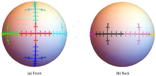
Let $E_0={\mathbb{S}}^2:=\left\{(cos\varphi cos\theta ,cos\varphi sin\theta ,sin\varphi ):\theta \in [-\pi ,\pi ],\varphi \in [-\pi /2,\pi /2]\right\}$ be a 2-sphere, where θ is the azimuthal angle and ϕ is the polar angle. For points on $E_0$, we compress their polar angles by 1/4 and their azimuthal angles by 1/7. Denote the resulting map by $R_1$. We rotate the image of $R_1$ about the z-axis by $-2\pi /7$, $-4\pi /7$, $-6\pi /7$, $2\pi /7$, $4\pi /7$, and $6\pi /7$ to obtain $R_2$, $R_3$, $R_4$, $R_5$, $R_6$, and $R_7$, respectively. We rotate the image of $R_1$ about the y-axis by $-5\pi /21$ and $5\pi /21$ to get $R_8$ and $R_9$, respectively. Then ${\left\{R_t\right\}}_{t=1}^9$ is an IRS on $E_0$ and is post critically finite (see, e.g., [27]). The attractor is shown in Figure 6.

Figure 6. The attractor of ${\left\{R_t\right\}}_{t=1}^9$ in Example 5.

The following example illustrates how to obtain the box dimension of an IRS attractor.

Example 6.

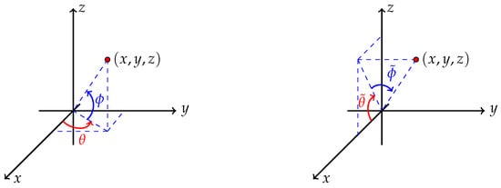
Let $E_0={\mathbb{S}}^2$ and let ${\mathbb{S}}_{+}^2:=\{(x,y,z):x\ge 0\}$. We use the following two different parameterizations for ${\mathbb{S}}^2$ and ${\mathbb{S}}_{+}^2$:

$$\begin{array}{cc}\hfill & \{(\theta ,\varphi ):=(cos\varphi cos\theta ,cos\varphi sin\theta ,sin\varphi ):\theta \in [-\pi ,\pi ],\varphi \in [-\pi /2,\pi /2]\}\mathrm{for}{\mathbb{S}}^2,\hfill \\ \hfill & \{(\tilde{\theta },\tilde{\varphi }):=(cos\tilde{\varphi }cos\tilde{\theta },sin\tilde{\varphi },cos\tilde{\varphi }sin\tilde{\theta }):\tilde{\theta }\in [-\pi /2,\pi /2],\tilde{\varphi }\in [-\pi /2,\pi /2]\}\mathrm{for}{\mathbb{S}}_{+}^2.\hfill \end{array}$$

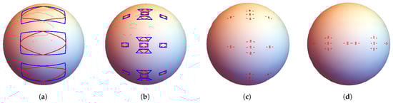
Here, we continue to call θ, $\tilde{\theta }$ azimuthal angles, and ϕ, $\tilde{\varphi }$ polar angles (see Figure 7). Let $R_1$ be a relation obtained as follows. First, compress the azimuthal angle θ by 1/6 using a relation which we denote by $f_1$. Next, we compose $f_1$ with a compression ${\tilde{f}}_1$ of the azimuthal angle $\tilde{\theta }$ by 1/6 to obtain $R_1$. We compose $R_1$ with rotations about the z-axis by $-5\pi /6$ and $5\pi /6$ to obtain $R_2$ and $R_3$, respectively. We compose $R_1$ with rotations about the y-axis by $-\pi /4$ and $\pi /4$ to get $R_4$ and $R_5$, respectively. ${\left\{R_t\right\}}_{t=1}^5$ is an IRS on $E_0$ and satisfies (SSC) (see Figure 8). The images of $E_0$ under the iterations of ${\left\{R_t\right\}}_{t=1}^5$ are closed regions enclosed by the red curves in Figure 8. Let K be the associated attractor. Then

$${dim}_{\mathrm{B}}\left(K\right)={\displaystyle \frac{log5}{log6}}\approx 0.898244.$$

Figure 7. The polar and azimuthal angles in the two parameterizations in Example 6.

Figure 8. The IRS ${\left\{R_t\right\}}_{t=1}^5$ in Example 6. Regions enclosed by the red curves are images of $E_0$ under the iterations of ${\left\{R_t\right\}}_{t=1}^5$. (a) The first iteration. $G_1^1$, $G_1^4$, and $G_1^5$ denote the middle, top, and bottom blue regions enclosed by the blue curves, respectively ($G_1^2$ and $G_1^3$ not shown). (b) The second iteration. Figures (c,d) show rough approximations to the front and back of the attractor.

Proof of Example 6.

Let $G_1^1$ be the region in the middle of Figure 8a enclosed by the blue curves, where the two curves on the left and right are, respectively,

$$\begin{array}{cc}\hfill & \left\{(-\pi /6,\varphi ):\varphi \in \left[-{tan}^{-1}\left(\sqrt{3}-{\displaystyle \frac{3}{2}}\right),{tan}^{-1}\left(\sqrt{3}-{\displaystyle \frac{3}{2}}\right)\right]\right\}\mathrm{and}\hfill \\ \hfill & \left\{(\pi /6,\varphi ):\varphi \in \left[-{tan}^{-1}\left(\sqrt{3}-{\displaystyle \frac{3}{2}}\right),{tan}^{-1}\left(\sqrt{3}-{\displaystyle \frac{3}{2}}\right)\right]\right\},\hfill \end{array}$$

and the two curves on the top and bottom are

$$\begin{array}{cc}\hfill & \left\{(-\pi /12,\tilde{\varphi }):\tilde{\varphi }\in \left[-{sin}^{-1}\left({\displaystyle \frac{1}{\sqrt{25-12\sqrt{3}}}}\right),{sin}^{-1}\left({\displaystyle \frac{1}{\sqrt{25-12\sqrt{3}}}}\right)\right]\right\}\mathrm{and}\hfill \\ \hfill & \left\{(\pi /12,\tilde{\varphi }):\tilde{\varphi }\in \left[-{sin}^{-1}\left({\displaystyle \frac{1}{\sqrt{25-12\sqrt{3}}}}\right),{sin}^{-1}\left({\displaystyle \frac{1}{\sqrt{25-12\sqrt{3}}}}\right)\right]\right\},\hfill \end{array}$$

respectively. We rotate $G_1^1$ about the z-axis by $-5\pi /6$ and $5\pi /6$ to obtain $G_1^2$ and $G_1^3$, respectively. We rotate $G_1^1$ about the y-axis by $-\pi /4$ and $\pi /4$ to get $G_1^4$ and $G_1^5$, respectively. Note that for each t, $R_t\left(E_0\right)\subseteq G_1^t$ and the boundary of $G_1^1$ intersects that of $R_t\left(E_0\right)$ at exactly four points (see Figure 8a). To compute the box dimension of K, we define a sequence $\left\{G_n\right\}$ of covers of K as follows. Let $G_1:={\bigcup }_{t=1}^5{G}_1^t$. For all $n\ge 2$, define

$$\begin{array}{c}\hfill G_n^{t_1\cdots t_n}:=R_t\left(G_{n-1}^{t_1\cdots t_{n-1}}\right),t_1,\dots ,t_n\in \{1,\dots ,5\}\mathrm{and}{G}_n:=\bigcup _{t_1,\dots ,t_n=1}^5{G}_n^{t_1\cdots t_n}.\end{array}$$

We need to compute the maximum diameter of the sets in each cover.

First, we find the maximum horizontal compression ratio. Let $A=(\theta ,\varphi )$ and $B=(-\theta ,\varphi )$ be two points in $G_1^4$, where $\theta >0$. Then $A^{\prime }:=f_1\left(A\right)=(\theta /6,\varphi )$ and $B^{\prime }:=f_1\left(B\right)=(-\theta /6,\varphi )$. Let $d_E$ and $d_M$ denote the Euclidean and Riemannian distances, respectively. Then $d_E(A,B)=2cos\varphi sin\theta$. Hence

$$\begin{array}{c}\hfill {\displaystyle \frac{d_E(A^{\prime },B^{\prime })}{d_E(A,B)}}={\displaystyle \frac{sin(\theta /6)}{sin\theta }}.\end{array}$$

Now let $\theta$ and $\varphi$ vary while fixing the Euclidean distance between $A(\theta ,\varphi )$ and $B(-\theta ,\varphi )$. Note that the larger the value of $\left|\varphi \right|$ (the absolute value of the latitude of A and B), the larger the value of $\theta$. To prove that as $\varphi \in [0,\pi /2)$ increases, the ratio $d_E(A^{\prime },B^{\prime })/d_E(A,B)$ also increases, define $f\left(x\right):=sin(x/6)/sinx$, where $x\in (0,\pi /2)$. Note that

$$\begin{array}{cc}\hfill & f^{\prime }\left(x\right)={\displaystyle \frac{(sinxcos(x/6\left)\right)/6-sin(x/6)cosx}{{sin}^{2}x}}\mathrm{and}\hfill \\ \hfill & {\displaystyle \frac{d}{dx}}(sinxcos(x/6)-6sin(x/6)cosx)={\displaystyle \frac{35}{6}}sin(x/6)sinx>0.\hfill \end{array}$$

Hence, $f\left(x\right)$ is increasing. Therefore, as the latitude increases while keeping the distance between $A(\theta ,\varphi )$ and $B(-\theta ,\varphi )$ fixed, the value of $\theta$ increases, and thus the ratio $d_E(A^{\prime },B^{\prime })/d_E(A,B)$ increases. Let

$$\begin{array}{c}\hfill h\left({\varphi }_1\right):={tan}^{-1}\left({\displaystyle \frac{2cos{\varphi }_1}{\sqrt{6}cos{\varphi }_1-2\sqrt{2}sin{\varphi }_1}}\right).\end{array}$$

A direct calculation shows that the right boundary curve of $G_1^4$ is

$$\begin{array}{cc}\hfill & \left\{\left(h\left({\varphi }_1\right),{sin}^{-1}\left({\displaystyle \frac{\sqrt{6}cos{\varphi }_1+2\sqrt{2}sin{\varphi }_1}{4}}\right)\right):{\varphi }_1\in \left[-{tan}^{-1}\left(\sqrt{3}-{\displaystyle \frac{3}{2}}\right),{tan}^{-1}\left(\sqrt{3}-{\displaystyle \frac{3}{2}}\right)\right]\right\}.\hfill \end{array}$$

We can prove that for ${\varphi }_1\in [-{tan}^{-1}(\sqrt{3}-3/2),{tan}^{-1}(\sqrt{3}-3/2)]$, $h\left({\varphi }_1\right)$ is increasing. Thus the maximum value of $\theta$ and $\varphi$ for the points in $G_1^4$ are, respectively,

$$\begin{array}{c}\hfill {tan}^{-1}\left({\displaystyle \frac{\sqrt{2}}{3-\sqrt{3}}}\right)\approx 0.839876\mathrm{and}{sin}^{-1}\left({\displaystyle \frac{3(\sqrt{3}-1)}{\sqrt{50-24\sqrt{3}}}}\right)\approx 0.857731.\end{array}$$

Hence the maximum value of $d_E(A^{\prime },B^{\prime })/d_E(A,B)$ is $c_{h,1}$, where

$$\begin{array}{c}\hfill c_{h,1}:=\sqrt{7-3\sqrt{3}}sin\left({\displaystyle \frac{1}{6}}{tan}^{-1}\left({\displaystyle \frac{\sqrt{2}}{3-\sqrt{3}}}\right)\right)\approx 0.187389.\end{array}$$

(32)

Let $({\theta }_n,{\varphi }_n):=f_1^n\left(A\right)$, where $A\in G_1^4$. Then ${lim}_{n\to \infty }{\theta }_n=0$. Thus,

$$\begin{array}{c}\hfill \underset{n\to \infty }{lim}{\displaystyle \frac{sin({\theta }_n/6)}{sin{\theta }_n}}={\displaystyle \frac{1}{6}}<c_{h,1}.\end{array}$$

(33)

If $A,B\in G_1\setminus G_1^4$, similar arguments show that the maximum horizontal compression ratio is $c_{h,1}$.

Next, we find the maximum vertical compression ratio. Let $\tilde{A}=(\tilde{\theta },\tilde{\varphi })$ and $\tilde{B}=(-\tilde{\theta },\tilde{\varphi })$ be two points in $G_1^1$, where $\tilde{\theta }>0$. When the azimuthal angle $\tilde{\theta }$ is compressed by 1/6 in the vertical direction, the images of $\tilde{A}$ and $\tilde{B}$ are $\widetilde{A^{\prime }}=(\tilde{\theta }/6,\tilde{\varphi })$ and $\widetilde{B^{\prime }}=(-\tilde{\theta }/6,\tilde{\varphi })$, respectively. Hence, $d_E(\widetilde{A^{\prime }},\widetilde{B^{\prime }})/d_E(\tilde{A},\tilde{B})=sin(\tilde{\theta }/6)/sin\tilde{\theta }$. For points $(\tilde{\theta },\tilde{\varphi })$ in $G_1^1$, as one varies $\tilde{\varphi }$ while keeping $\tilde{\theta }$ constant so that $(\tilde{\theta },\tilde{\varphi })$ remains within $G_1^1$, the maximum possible values of $\tilde{\theta }$ and $\tilde{\varphi }$ are, respectively,

$$\begin{array}{c}\hfill \pi /12\approx 0.261799\mathrm{and}{sin}^{-1}\left({\displaystyle \frac{1}{\sqrt{25-12\sqrt{3}}}}\right)\approx 0.508719.\end{array}$$

Thus the maximum value of $d_E(\widetilde{A^{\prime }},\widetilde{B^{\prime }})/d_E(\tilde{A},\tilde{B})$ is

$$\begin{array}{c}\hfill c_{v,1}:={\displaystyle \frac{2\sqrt{2}sin(\pi /72)}{\sqrt{3}-1}}\approx 0.168532<c_{h,1}.\end{array}$$

Let $({\tilde{\theta }}_n,{\tilde{\varphi }}_n):={\tilde{f}}_1^n\left(\tilde{A}\right)$, where $\tilde{A}\in G_1^1$. Then ${lim}_{n\to \infty }{\tilde{\theta }}_n=0$. Thus,

$$\begin{array}{c}\hfill \underset{n\to \infty }{lim}{\displaystyle \frac{sin({\tilde{\theta }}_n/6)}{sin{\tilde{\theta }}_n}}={\displaystyle \frac{1}{6}}<c_{v,1}.\end{array}$$

For $A,B\in G_1\setminus G_1^1$, similar arguments show that the maximum vertical compression ratio is $c_{v,1}$. Let $c_{h,n}$ and $c_{v,n}$ be the horizontal and vertical compression ratios of the $n^{th}$ iteration, respectively. Using a similar proof as that for $n=1$, we have $c_{v,n}<c_{h,n}$ for any $n\ge 2$.

Finally, fix $t\in \{1,\dots ,5\}$. For any two points $C_1:=({\theta }_1,{\varphi }_1)$ and $D_1:=({\theta }_2,{\varphi }_2)$ in $G_1^t$, where ${\theta }_1\ne {\theta }_2$ or ${\varphi }_1\ne {\varphi }_2$, let $▵C_1{D}_1{F}_1$ be a Euclidean right triangle with $F_1\in E_0$. Then $d_E(C_1,D_1)=\sqrt{d_E^2(C_1,F_1)+d_E^2(D_1,F_1)}$. Let $C_2:=R_t\left(C_1\right)$, $D_2:=R_t\left(D_1\right)$, and $F_2:=R_t\left(F_1\right)$. Then $▵C_2{D}_2{F}_2$ is also a Euclidean right triangle. Hence

$$\begin{array}{c}\hfill d_E(C_2,D_2)\le \sqrt{c_{h,1}^2{d}_E^2(C_1,F_1)+c_{v,1}^2{d}_E^2(D_1,F_1)}\le c_{h,1}{d}_E(C_1,D_1).\end{array}$$

Let $C_{n+1}$ and $D_{n+1}$ denote the $n^{th}$ iterates, under $R_t$, of the points $C_1$ and $D_1$, respectively. Then

$$\begin{array}{c}\hfill d_E(C_{n+1},D_{n+1})\le c_{h,1}\cdots c_{h,n}{d}_E(C_1,D_1).\end{array}$$

(34)

In view of (33), $\left\{c_{h,n}\right\}$ is monotone decreasing and tends to $1/6$ as n tends to infinity. Let ${\mathrm{diam}}_E\left(G_n^t\right)$ and ${\mathrm{diam}}_M\left(G_n^t\right)$ denote the diameters of $G_n^t$ in the Euclidean and Riemannian metrics, respectively. Define

$$\begin{array}{cc}\hfill & {\delta }_{E,n}:=max\{{\mathrm{diam}}_E\left(G_n^{t_1\cdots t_n}\right):t_1,\dots ,t_n\in \{1,\dots ,5\}\}\mathrm{and}\hfill \\ & {\delta }_{M,n}:=max\{{\mathrm{diam}}_M\left(G_n^{t_1\cdots t_n}\right):t_1,\dots ,t_n\in \{1,\dots ,5\}\}.\hfill \end{array}$$

By (34), there exist constants ${\kappa }_1,{\kappa }_2>0$ such that

$$\begin{array}{c}\hfill {\kappa }_1{\left({\displaystyle \frac{1}{6}}\right)}^n\le {\delta }_{E,n}\le {\kappa }_2(c_{h,1}\cdots c_{h,n}),\end{array}$$

(35)

where the first inequality can be obtained easily. Let O be the the center of $E_0$. For any $A,B\in E_0$, let $\alpha :=\angle AOB$. Then

$$\begin{array}{c}\hfill d_M(A,B)={\displaystyle \frac{\alpha }{2sin(\alpha /2)}}{d}_E(A,B).\end{array}$$

(36)

Let ${\alpha }_n:=\angle C_{n}O{D}_n$ and ${\alpha }_{n+1}:=\angle C_{n+1}O{D}_{n+1}$. Combining (35) and (36), we have

$$\begin{array}{c}\hfill {\kappa }_1{\displaystyle \frac{{\alpha }_n}{2sin({\alpha }_n/2)}}{\left({\displaystyle \frac{1}{6}}\right)}^n\le {\delta }_{M,n}={\displaystyle \frac{{\alpha }_n}{2sin({\alpha }_n/2)}}{\delta }_{E,n}\le {\kappa }_2{\displaystyle \frac{{\alpha }_n}{2sin({\alpha }_n/2)}}(c_{h,1}\cdots c_{h,n}).\end{array}$$

(37)

Note that $\alpha \to 0$ as n, the level of iteration, tends to infinity. Thus,

$$\begin{array}{c}\hfill \underset{n\to \infty }{lim}{\displaystyle \frac{{\alpha }_n}{2sin({\alpha }_n/2)}}=1.\end{array}$$

(38)

By the definition of ${\left\{R_t\right\}}_{t=1}^5$, K can be covered by a minimum of $5^n$ sets (say, the $G_n^t$’s), each with Riemannian diameter no more than ${\delta }_{M,n}$. Hence $N_{{\delta }_{M,n}}\left(K\right)=5^n$. Using the fact that the sequence $\left\{{\delta }_{M,n}\right\}$ is slowly decreasing, we have

$$\begin{array}{cc}\hfill {\overline{dim}}_{\mathrm{B}}\left(K\right)=& \underset{n\to \infty }{\overline{lim}}{\displaystyle \frac{log{5}^n}{-log{\delta }_{M,n}}}\ge \underset{n\to \infty }{lim}{\displaystyle \frac{log{5}^n}{-log{\kappa }_1-log\left(\frac{{\alpha }_n}{2sin({\alpha }_n/2)}\right)-log{(1/6)}^n}}\left(\mathrm{by}\left(37\right)\right)\hfill \\ \hfill =& {\displaystyle \frac{log5}{log6}}\approx 0.898244\left(\mathrm{by}\left(38\right)\right).\hfill \end{array}$$

Similarly, we have ${\underline{dim}}_{\mathrm{B}}\left(K\right)\ge log5/log6$. On the other hand, for any $ϵ>0$, we let

$${\delta }_n:={\kappa }_2{\displaystyle \frac{{\alpha }_n}{2sin({\alpha }_n/2)}}{\left({\displaystyle \frac{1}{6}}+ϵ\right)}^n.$$

Then, in view of (34) and (37), for all n sufficiently large,

$${\delta }_n\ge {\kappa }_2{\displaystyle \frac{{\alpha }_n}{2sin({\alpha }_n/2)}}(c_{h,1}\cdots c_{h,n})\ge {\delta }_{M,n}$$

and hence $N_{{\delta }_n}\left(K\right)\le 5^n$. Thus,

$$\begin{array}{cc}\hfill {\overline{dim}}_{\mathrm{B}}\left(K\right)=& \underset{n\to \infty }{\overline{lim}}{\displaystyle \frac{log{N}_{{\delta }_n}\left(K\right)}{-log{\delta }_n}}\le \underset{n\to \infty }{lim}{\displaystyle \frac{log{5}^n}{-log{\kappa }_2-log\left(\frac{{\alpha }_n}{2sin({\alpha }_n/2)}\right)-log{(1/6+ϵ)}^n}}\hfill \\ \hfill =& {\displaystyle \frac{log5}{-log(1/6+ϵ)}}.\hfill \end{array}$$

Letting $ϵ\to 0$ yields ${\overline{dim}}_{\mathrm{B}}\left(K\right)\le log5/log6$. Similarly, we have ${\underline{dim}}_{\mathrm{B}}\left(K\right)\le log5/log6$. This completes the proof.  □

8. Conclusions

Fractals on Riemannian manifolds generated by non-contractive or multivalued relations cannot be described by iterated function systems. We introduce the notion of an iterated relation system to describe these fractals. To compute the Hausdorff dimension of an IRS attractor, we introduce the notion of a graph-directed iterated function system associated with an IRS and prove that the IRS attractor can be identified with the attractor of the associated GIFS. In addition, we formulate conditions under which a GIFS associated with an IRS exists. This allows us to obtain a formula for the Hausdorff dimension of an IRS attractor on a locally Euclidean Riemannian manifold, under either the graph open set condition or the graph finite type condition. Finally, we illustrate how to obtain the box dimension of an IRS attractor on ${\mathbb{S}}^2$.

References

- Strichartz, R.S. Self-similarity on nilpotent Lie groups. Contemp. Math. 1992, 140, 123–157. [Google Scholar]
- Balogh, Z.M.; Tyson, J.T. Hausdorff dimensions of self-similar and self-affine fractals in the Heisenberg group. Proc. Lond. Math. Soc. 2005, 91, 153–183. [Google Scholar] [CrossRef]
- Barnsley, M.F.; Vince, A. Real projective iterated function systems. J. Geom. Anal. 2012, 22, 1137–1172. [Google Scholar] [CrossRef]
- Hossain, A.; Akhtar, M.N.; Navascués, M.A. Fractal dimension of fractal functions on the real projective plane. Fractal Fract. 2023, 7, 510. [Google Scholar] [CrossRef]
- Hossain, A.; Akhtar, M.N.; Navascués, M.A. Fractal interpolation on the real projective plane. Numer. Algorithms 2024, 96, 557–582. [Google Scholar] [CrossRef]
- Ngai, S.-M.; Xu, Y.Y. Separation conditions for iterated function systems with overlaps on Riemannian manifolds. J. Geom. Anal. 2023, 33, 262. [Google Scholar] [CrossRef]
- Thangaraj, C.; Easwaramoorthy, D.; Selmi, B.; Chamola, B.P. Generation of fractals via iterated function system of Kannan contractions in controlled metric space. Math. Comput. Simul. 2024, 222, 188–198. [Google Scholar] [CrossRef]
- Cui, M.; Selmi, B.; Li, Z. Expansive measures of nonautonomous iterated function systems. Qual. Theory Dyn. Syst. 2025, 24, 60. [Google Scholar] [CrossRef]
- Balogh, Z.M.; Rohner, H. Self-similar sets in doubling spaces. Ill. J. Math. 2007, 51, 1275–1297. [Google Scholar] [CrossRef]
- Hutchinson, J.E. Fractals and self-similarity. Indiana Univ. Math. J. 1981, 30, 713–747. [Google Scholar] [CrossRef]
- Wu, D.; Yamaguchi, T. Hausdorff dimension of asymptotic self-similar sets. J. Geom. Anal. 2017, 4, 339–368. [Google Scholar] [CrossRef]
- Ngai, S.-M.; Wang, Y. Hausdorff dimension of self-similar sets with overlaps. J. Lond. Math. Soc. 2001, 2, 655–672. [Google Scholar] [CrossRef]
- Jin, N.; Yau, S.S.T. General finite type IFS and M-matrix. Commun. Anal. Geom. 2005, 13, 821–843. [Google Scholar]
- Lau, K.-S.; Ngai, S.-M. A generalized finite type condition for iterated function systems. Adv. Math. 2007, 208, 647–671. [Google Scholar] [CrossRef]
- Akhtar, M.N.; Hossain, A. Stereographic metric and dimensions of fractals on the sphere. Results Math. 2022, 77, 213. [Google Scholar] [CrossRef]
- Akhtar, M.N.; Prasad, M.G.P.; Navascués, M.A. More general fractal functions on the sphere. Mediterr. J. Math. 2019, 16, 134. [Google Scholar] [CrossRef]
- Navascués, M.A. Fractal functions on the sphere. J. Comput. Anal. Appl. 2007, 9, 257–270. [Google Scholar]
- Vince, A. Möbius iterated function systems. Trans. Amer. Math. Soc. 2013, 365, 491–509. [Google Scholar] [CrossRef]
- Mauldin, R.D.; Williams, S.C. Hausdorff dimension in graph directed constructions. Trans. Amer. Math. Soc. 1988, 309, 811–829. [Google Scholar] [CrossRef]
- Edgar, G.A. Measure, Topology, and Fractal Geometry; Springer: New York, NY, USA, 2008. [Google Scholar]
- Petersen, P. Riemannian Geometry; Graduate Texts in Mathematics; Springer: Cham, Switzerland, 2006; Volume 171. [Google Scholar]
- Jost, J. Riemannian Geometry and Geometric Analysis; Universitext; Springer: Cham, Switzerland, 2017. [Google Scholar]
- Hebey, E. Sobolev Spaces on Riemannian Manifolds; Springer: Berlin/Heidelberg, Germany, 1996. [Google Scholar]
- Chavel, I. Riemannian Geometry: A Modern Introduction; Cambridge University Press: Cambridge, UK, 2006. [Google Scholar]
- Falconer, K.J. Fractal Geometry: Mathematical Foundations and Applications, 2nd ed.; John Wiley: Hoboken, NJ, USA, 2014. [Google Scholar]
- Das, M.; Ngai, S.-M. Graph-directed iterated function systems with overlaps. Indiana Univ. Math. J. 2004, 53, 109–134. [Google Scholar] [CrossRef]
- Kigami, J. Analysis on Fractals; Cambridge University Press: Cambridge, UK, 2001. [Google Scholar]
Disclaimer/Publisher’s Note: The statements, opinions and data contained in all publications are solely those of the individual author(s) and contributor(s) and not of MDPI and/or the editor(s). MDPI and/or the editor(s) disclaim responsibility for any injury to people or property resulting from any ideas, methods, instructions or products referred to in the content. |
© 2025 by the authors. Licensee MDPI, Basel, Switzerland. This article is an open access article distributed under the terms and conditions of the Creative Commons Attribution (CC BY) license (https://creativecommons.org/licenses/by/4.0/).