Hybrid Dynamic Event-Triggered Interval Observer Design for Nonlinear Cyber–Physical Systems with Disturbance

Abstract

This paper investigates the state estimation problem for nonlinear cyber–physical systems (CPSs). To conserve system resources, we propose a novel hybrid dynamic event-triggered mechanism (ETM) that prevents the occurrence of Zeno behavior. This work is based on designing an interval observer under the hybrid dynamic ETM to solve the state reconstruction problem of Lipschitz nonlinear CPSs subject to disturbances. That is, the designed triggering mechanism is integrated into the design of the Interval Observer (IO), resulting in a hybrid dynamic event-triggered interval observer (HDETIO), and the system stability and robustness are proved using a Lyapunov function, demonstrating that the observer can effectively provide interval estimation for CPSs with nonlinearity and disturbances. Compared to existing work, the primary contribution of this work is its ability to pre-specify the minimum inter-event time (MIET) and apply it to interval state estimation, enhancing its practicality for real-world physical systems. Finally, the correctness and effectiveness of the designed hybrid dynamic ETM and IO framework are validated with an example.

1. Introduction

With the rapid advancements in computer technology, network communication, and control theory, CPSs have enabled a profound integration of physical entities with computation, communication, and control functions [1]. These systems have found wide applications in fields such as smart grids [2], aerospace engineering [3], and robotic systems [4]. Concurrently, the ongoing progression of Industry 4.0 has greatly enhanced the flexibility and intelligence of CPSs. However, in practical engineering applications, CPSs often face limitations in accessing complete state parameters due to the limitations of measurement techniques and resource constraints. This brings challenges to the implementation of some CPSs functions, such as observer-based state feedback control and distributed coordinated control. Therefore, solving the state estimation problem in CPSs is significant and has drawn a great deal of attention from researchers.

In research related to the state estimation problem of CPSs, the predominant methods include observer techniques and filtering approaches. For instance, ref. [5] explored the development of a hybrid state estimation mechanism that integrates discrete and continuous observation techniques and demonstrates its application in the field of electric vehicle technology. Ref. [6] studied the stochastic stability of state estimation based on Kalman filtering within lossy network environments. Ref. [7] primarily focused on attack detection and security state estimation of CPSs under finite-time attacks. Due to the presence of various unknown signals in the system, which can generally be classified as random signals or interval signals, existing observers can be categorized into point estimators and IOs. The IOs, first proposed by J.L. Gouzé et al. [8], have been provided with a structural framework. Subsequently, researchers introduced coordinate transformation methods into switching systems and constructed a series of interval observers for switching systems [9,10], relaxing the limitations of interval observer design conditions. Furthermore, for CPSs, IOs not only solve the state estimation problem, but also provide an interval range of states, making them more applicable to real-world engineering scenarios. With the continuous innovation and development of IO design techniques, scholars have proposed numerous set-membership estimation methods to design such observers. For example, polytopes [11], ellipsoids [12], and zonotopes [13] can all be used to enclose the actual state of the system at each moment. Additionally, IOs exhibit good robustness against certain nonlinearities [14] and unknown disturbances [15]. Ref. [16] investigated the stealthiness of attack strategies against ${\chi }^2$ detectors for CPSs under covert deceptive attacks and achieved interval estimation of the state through H_∞ technology and reachable set analysis. Consequently, IOs are of significant practical importance in the study of CPSs reconstruction problems.

On the other hand, in CPSs, efficiently utilizing computational and communication resources is a critical issue. Consequently, the ETM has gradually garnered significant research attention. The core concept of the ETM is that it does not trigger control actions at fixed time intervals; instead, it relies on changes in system states or specific events to trigger actions. This mechanism can reduce redundant data transmission caused by periodic sampling, particularly when system states do not change significantly, thereby markedly decreasing energy consumption and network burden. A periodic ETM was previously proposed in [17], which also studied static state feedback and dynamic output-based controllers based on the periodic ETM. To further conserve energy while ensuring system performance, an additional variable was introduced in [18], resulting in the dynamic ETM. Consequently, the dynamic ETM has begun to attract preliminary research interest, as stated in [19,20,21,22]. Among these studies, ref. [19] applied the dynamic ETM to a singular system affected by random network attacks and designed an H_∞ controller to enhance the robustness of the singular system. Meanwhile, ref. [20] integrated model-based CPSs with the dynamic ETM to investigate the L₂ gain performance of CPSs in the presence of DoS attacks, while also considering the implications of quantization. Additionally, ref. [23] introduced adaptive event-triggered control into nonlinear uncertain systems; an adaptive controller based on backstepping was designed to deal with the parametric uncertainties. At the same time, adaptive event triggering control [24] was applied to commercial mobile robots subject to input delay and limited communications. It provides a broader perspective on the applicability and scalability of the method.

Furthermore, the integration of ETM into CPSs introduces a critical challenge: excluding Zeno behavior, which refers to the phenomenon of infinite actuator triggering within a limited time. Reference [25] explored the consistency control of multi-agent systems utilizing distributed ETM, addressing the exclusion of Zeno behavior by ensuring that the interval between any successive trigger events exceeds a constant positive value. In [26], Zeno behavior was excluded through a proof by contradiction. However, due to the inherent minimum reaction time of practical hardware and the theoretical MIET potentially being a very small positive number, Zeno behavior can still occur. Therefore, an effective method to eliminate the limitations of Zeno behavior is to improve the trigger conditions by pre-designing a MIET that ensures a strictly positive MIET and to meet the demands of practical applications. Consequently, a new hybrid dynamic ETM was proposed in [27]. Reference [28] extended this hybrid dynamic ETM to multi-agent systems, successfully achieving consensus control. However, the issue of interval estimation in CPSs based on hybrid dynamic ETM has not been studied yet.

Therefore, this paper proposes a novel HDETIO design method for state reconstruction and resource optimization in nonlinear CPSs with disturbance. It addresses the state estimation problem of CPSs under a hybrid dynamic ETM. By reducing the number of executions of the trigger while ensuring the estimation accuracy, it achieves the effect of optimizing resources. At the same time, it also avoids the infinite triggering fault of the trigger caused by the insufficiency of actual engineering hardware. The primary approach is to reduce the observer’s reliance on the original systems’ output through the hybrid dynamic ETM, thereby designing an IO using the positive system method and analyzing its stability. The contributions of this paper mainly lie in two aspects: Firstly, the introduction of a novel hybrid dynamic ETM that prevents Zeno behavior and allows for the pre-specification of the MIET during the design process. Secondly, a novel HDETIO is constructed, which not only achieves interval estimation of CPSs, but also conserves system resources. The structure of this paper is organized as follows: Section 2 elaborates on fundamental concepts. Section 3 presents the main conclusions, with a primary focus on the design of HDETIO and the stability analysis of CPSs. Section 4 demonstrates their effectiveness through numerical simulations. Finally, the Conclusions are summarized.

Notation:For a matrix $\mathcal{H}\in R^{m\times n}$, ${\mathcal{H}}^T$ is utilized to represent the transpose of matrix $\mathcal{H}$, and we define $\mathcal{H}\succ 0(\prec 0)$ to indicate that $\mathcal{H}$ is a positive definite (negative definite) matrix, respectively. We also define ${\mathcal{H}}^{+}=max(\mathcal{H},0)$ and ${\mathcal{H}}^{-}={\mathcal{H}}^{+}-\mathcal{H}$. The symbol $\Vert ·\Vert$ denotes the Euclidean norm. For a square matrix $\mathrm{{\rm Y}}$, the expression ${\lambda }_{\mathrm{{\rm Y}}max}$ (${\lambda }_{\mathrm{{\rm Y}}min}$) represents the maximum (minimum) eigenvalue of $\mathrm{{\rm Y}}$. In symmetric block matrices, symmetric terms can be represented by *. $I_n$ is the n dimensional identity matrix.

2. Preliminaries

To begin with, we consider a nonlinear continuous system as follows,

$$\left\{\begin{array}{c}\begin{array}{c}\dot{x}\left(t\right)=Ax\left(t\right)+Bu\left(t\right)+F\left(x\left(t\right)\right)+Dd\left(t\right),\hfill \\ y\left(t\right)=Cx\left(t\right),\hfill \end{array}\end{array}\right.$$

(1)

where $x\left(t\right)\in R^{n_x}$ and $u\left(t\right)\in R^{n_u}$ are the state and control input. $F\left(x\left(t\right)\right)\in R^{n_x}$ is the nonlinear term. $y\left(t\right)\in R^{n_y}$ and $d\left(t\right)\in R^{n_d}$ represent the output and unknown process noise.

In an effort to optimize and significantly boost the performance of our resources, we have implemented an innovative ETM. This mechanism is designed to activate certain processes or operations only after specific conditions are met and a set triggering interval time ${\tau }_{ETI}^{min}$ has elapsed. This strategy aims to cut down on pointless calculations and communications, thereby conserving energy and improving the overall efficiency of the system. The hybrid dynamic ETM is presented as follows:

$$\left\{\begin{array}{c}\begin{array}{c}{t}_{k+1}=inf\{t\ge t_k+{\tau }_{\mathit{ETI}}^{min}|\Phi (y\left(t\right),e_y\left(t\right))\ge \eta \left(t\right)\},\hfill \\ \dot{\eta }\left(t\right)=-\lambda \eta \left(t\right)-\Phi (y\left(t\right),e_y\left(t\right)),\hfill \end{array}\end{array}\right.$$

(2)

where $\lambda >0$, $\eta \left(0\right)>0$, $\Phi (y\left(t\right),e_y\left(t\right))=\alpha \left[e_y^T\left(t\right)\overline{P}{e}_y\left(t\right)-\beta y^T\left(t\right)Qy\left(t\right)\right]$, $e_y\left(t\right)=y\left(t\right)-y\left(t_k\right)$, and ${\tau }_{\mathit{ETI}}^{min}$ is the pre-specified minimum triggering interval and $y\left(t_k\right)$ is the output transmitted after triggering. The initial condition is $t_0=0$ and $\eta \left(t\right)$ is a bounded non-negative function.

Figure 1 illustrates the interval observer design framework based on the hybrid dynamic ETM. Within this system, the hybrid dynamic ETM mitigates the burden on communication and computational resources by reducing unnecessary data updates. The design of the interval observer takes into account the disturbances and event-driven impacts of CPSs, ensuring the stability and robustness of the system. The objective of this paper is to conduct research on the state estimation problem of CPSs within the hybrid dynamic ETM environment by designing an effective interval observer, thereby conserving the resources of the networked system.

Remark 1.

The hybrid dynamic ETM reverts to a static ETM under the condition where the minimum event-triggered interval ${\tau }_{\mathit{ETI}}^{min}$ is zero and the dynamic threshold function $\eta \left(t\right)$ is zero. In this scenario, the simplified form of ETM as shown below,

$$\begin{array}{c}{t}_{k+1}=inf\{t\ge t_k|\Phi (y\left(t\right),e_y\left(t\right))\ge 0\}.\hfill \end{array}$$

(3)

This represents a transition from a dynamic to a static triggering logic, highlighting the flexibility of the hybrid dynamic ETM framework to adapt to different system requirements. Furthermore, it is crucial to acknowledge that the hybrid dynamic ETM degrades to a dynamic ETM if, and only if, ${\tau }_{\mathit{ETI}}^{min}=0$. The following equations determine the dynamic ETM:

$$\left\{\begin{array}{c}\begin{array}{c}{t}_{k+1}=inf\{t\ge t_k|\Phi (y\left(t\right),e_y\left(t\right))\ge \eta \left(t\right)\},\hfill \\ \dot{\eta }\left(t\right)=-\lambda \eta \left(t\right)-\Phi (y\left(t\right),e_y\left(t\right)).\hfill \end{array}\end{array}\right.$$

(4)

These equations are the dynamic adjusted of the triggering condition according to the system state and the threshold function $\eta \left(t\right)$, which is influenced by the system performance and the chosen design parameter β. This degradation to DETM emphasizes the seamless transition of the hybrid dynamic ETM in response to specific operational constraints, providing a robust framework for event-triggered control systems.

Remark 2.

The configuration of the ETM is depicted in Figure 1. Within this proposed framework, the parameter ${\mathit{\tau }}_{\mathit{ETI}}^{min}>0$ is defined to ensure a minimum positive interval between triggers, thereby averting the occurrence of Zeno behavior. This is accomplished by incorporating a timer (refer to Figure 1) that measures the duration since the last triggering event. Additionally, as illustrated in Figure 1 and Equation (3), the triggering condition is determined using only local variables.

Remark 3.

Figure 2 shows the event-triggered interval for a case. If the depicted behavior is the result of either a static or dynamic ETM, the minimum triggering interval is determined after the mechanism has been activated. Conversely, if the behavior is derived from a hybrid dynamic ETM, the minimum interval is known prior to the triggering event and is established during the system design phase; all of the trigger interval times are above the red dashed line shown in Figure 2. This prior knowledge of the minimum interval allows for a more informed selection and design tailored to specific requirements.

Remark 4.

In the design of interval observers for linear continuous systems, it is essential to first ascertain that the system’s initial state and disturbances are bounded, as outlined in Assumption 1. This condition is typically satisfied in practical applications, and its constraint is considered negligible, which is the same as that in [9,14].

Lemma 1

([29]). Supposing that the function $\mathfrak{I}\left(x\right)$ exhibits global Lipschitz continuity and differentiability, it is then possible to identify two non-decreasing Lipschitz functions $g\left(x\right)$ and $\phi \left(x\right)$ that satisfy

$$\mathfrak{I}\left(x\right)=g\left(x\right)-\phi \left(x\right).$$

(5)

Lemma 2

([29]). Let the function $\mathfrak{I}\left(x\right)$ be defined in Lemma 1, it is possible to find a globally Lipschitz continuous function $\overline{\mathfrak{I}}(x_a,x_b)$ such that

$$\left\{\begin{array}{c}\begin{array}{c}{\displaystyle \overline{\mathfrak{I}}(x,x)=\mathfrak{I}\left(x\right),}\hfill \\ {\displaystyle \frac{\partial \overline{\mathfrak{I}}}{x_a}\ge 0,}\hfill \\ {\displaystyle \frac{\partial \overline{\mathfrak{I}}}{x_b}\le 0.}\hfill \end{array}\end{array}\right.$$

(6)

The preceding lemmas assist in establishing the bounds for $\mathfrak{I}(x,x)$:

$$\overline{\mathfrak{I}}(x^{-},x^{+})\le \mathfrak{I}(x,x)\le \overline{\mathfrak{I}}(x^{+},x^{-}).$$

(7)

Lemma 3

([29]). For $\mathfrak{I}\left(x\right)$, along with $\overline{\mathfrak{I}}(x^{+},x^{-})$ and $\overline{\mathfrak{I}}(x^{-},x^{+})$, as outlined in Lemma 2, there exist the constants ${\rho }_i(i=1,2,3,4)$, such that

$$\left\{\begin{array}{c}\begin{array}{c}\overline{\mathfrak{I}}(x^{+},x^{-})-\mathfrak{I}\left(x\right)\le {\rho }_1(x^{+}-x)+{\rho }_2(x-x^{-}),\hfill \\ \mathfrak{I}\left(x\right)-\mathfrak{I}(x^{-},x^{+})\le {\rho }_3(x^{+}-x)+{\rho }_4(x-x^{-}).\hfill \end{array}\end{array}\right.$$

(8)

Lemma 4

([30]). For a constant matrix $A\in R^{m\times n}$ and a vector $\varsigma \in R^n\in [{\varsigma }^{-},{\varsigma }^{+}]$, then

$$A^{+}{\varsigma }^{-}-A^{-}{\varsigma }^{+}\le A\varsigma \le A^{+}{\varsigma }^{+}-A^{-}{\varsigma }^{-}.$$

(9)

Lemma 5

([31]). If Equation (2) holds, then the event-triggered variable $\eta \left(t\right)>0$ at any time t.

Assumption 1.

The initial state $x\left(0\right)$ and the disturbances $d\left(t\right)$ of the system are bound.

Assumption 2.

If the function $F\left(x\right(t\left)\right)$ satisfies the Lipschitz condition and $F\left(0\right)=0$, there exists $\iota \in {\mathrm{N}}^{+}$, such that any $x_1,x_2\in {\mathbb{R}}^n$, and the following inequality holds

$$\parallel F\left(x_1\right)-F\left(x_2\right)\parallel \le \iota \parallel x_1-x_2\parallel .$$

(10)

3. Main Results

3.1. Design of the HDETIO Frame

Firstly, we design the following HDETIO frame:

$$\left\{\begin{array}{c}\begin{array}{cc}\hfill {\dot{\widehat{x}}}^{+}\left(t\right)=& A{\widehat{x}}^{+}\left(t\right)+Bu\left(t\right)+\overline{F}(x^{+}\left(t\right),x^{-}\left(t\right))+D^{+}{d}^{+}\left(t\right)-D^{-}{d}^{-}\left(t\right)\hfill \\ \hfill & +L(y\left(t_k\right)-C{\widehat{x}}^{+}\left(t\right))+L^{+}{e}_y^{+}\left(t\right)-L^{-}{e}_y^{-}\left(t\right),\hfill \\ \hfill {\dot{\widehat{x}}}^{-}\left(t\right)=& A{\widehat{x}}^{-}\left(t\right)+Bu\left(t\right)+\overline{F}(x^{-}\left(t\right),x^{+}\left(t\right))+D^{+}{d}^{-}\left(t\right)-D^{-}{d}^{+}\left(t\right)\hfill \\ \hfill & +L(y\left(t_k\right)-C{\widehat{x}}^{-}\left(t\right))+L^{+}{e}_y^{-}\left(t\right)-L^{-}{e}_y^{+}\left(t\right),\hfill \end{array}\end{array}\right.$$

(11)

where ${\widehat{x}}^{+}\left(t\right)$ and ${\widehat{x}}^{-}\left(t\right)$ are the estimation of $x\left(t\right)$ and L is the gain matrix of the system to be designed.

Theorem 1.

Suppose that $A-LC$ is a Metzler matrix and Assumption 1 holds, then

$${\widehat{x}}^{-}\left(t\right)\le x\left(t\right)\le {\widehat{x}}^{+}\left(t\right).$$

(12)

Proof. 

In the light of (9) and Assumption 1, we can draw the following conclusion:

$$\left\{\begin{array}{c}\begin{array}{cc}\hfill {\Sigma }_1=& \overline{F}(x^{+}\left(t\right),x^{-}\left(t\right))-F\left(x\left(t\right)\right)+D^{+}{d}^{+}\left(t\right)-D^{-}{d}^{-}\left(t\right)-Dd\left(t\right)\hfill \\ & -L{e}_y\left(t\right)+L^{+}{e}_y^{+}\left(t\right)-L^{-}{e}_y^{-}\left(t\right)\ge 0,\hfill \\ \hfill {\Sigma }_2=& F\left(x\left(t\right)\right)-\overline{F}(x^{-}\left(t\right),x^{+}\left(t\right))+Dd\left(t\right)-D^{+}{d}^{-}\left(t\right)+D^{-}{d}^{+}\left(t\right)\hfill \\ & -L^{+}{e}_y^{-}\left(t\right)+L^{-}{e}_y^{+}\left(t\right)+L{e}_y\left(t\right)\ge 0.\hfill \end{array}\end{array}\right.$$

(13)

In view of the ETM (2), we can define the error system as follows:

$$\left\{\begin{array}{c}\begin{array}{c}\hfill {e_x}^{+}\left(t\right)={\widehat{x}}^{+}\left(t\right)-x\left(t\right),\\ \hfill {e_x}^{-}\left(t\right)=x\left(t\right)-{\widehat{x}}^{-}\left(t\right).\end{array}\end{array}\right.$$

(14)

Subsequently, the error systems are transformed into the equations as below:

$$\left\{\begin{array}{c}\begin{array}{cc}\hfill {\dot{e}}_x^{+}\left(t\right)& =(A-LC)e_x^{+}\left(t\right)+{\Sigma }_1,\hfill \\ \hfill {\dot{e}}_x^{-}\left(t\right)& =(A-LC)e_x^{-}\left(t\right)+{\Sigma }_2.\hfill \end{array}\end{array}\right.$$

(15)

Based on (15), if $A-LC$ is a Metzler matrix, and under the fact that ${\widehat{x}}^{-}\left(0\right)\le x\left(0\right)\le {\widehat{x}}^{+}\left(0\right)$, $e^{+}\left(0\right)\ge 0$ and $e^{-}\left(0\right)\ge 0$, we conclude that ${\dot{e}}_x^{-}\left(t\right)$ and ${\dot{e}}_x^{-}\left(t\right)$ are non-negative. Therefore, one can obtain

$${\widehat{x}}^{-}\left(t\right)\le x\left(t\right)\le {\widehat{x}}^{+}\left(t\right),t\ge 0.$$

□

3.2. Stability Analysis of HDETIO

Defining $\xi \left(t\right)={\left[\begin{array}{c}({e_x}^{+}\left(t\right){)}^T{\left({e_x}^{-}\left(t\right)\right)}^T\end{array}\right]}^T$, then (15) can be written as

$$\dot{\xi }\left(t\right)=\tilde{A}\xi \left(t\right)+\tilde{F}\left(x\left(t\right)\right)+\tilde{D}d\left(t\right)+\tilde{L}{e}_y\left(t\right)+\tilde{E}g\left(t\right),$$

(16)

where

$$\tilde{A}=\left[\begin{array}{cc}A-LC& 0\\ 0& A-LC\end{array}\right],\tilde{F}\left(x\left(t\right)\right)=\left[\begin{array}{c}\overline{F}(x^{+}\left(t\right),x^{-}\left(t\right))-F\left(x\left(t\right)\right)\\ F\left(x\left(t\right)\right)-\overline{F}(x^{-}\left(t\right),x^{+}\left(t\right))\end{array}\right],$$

$$\tilde{D}=\left[\begin{array}{c}-D\\ D\end{array}\right],\tilde{L}=\left[\begin{array}{c}-L\\ L\end{array}\right],\begin{array}{c}\hfill \tilde{E}=\left[\begin{array}{cccc}{L}^{+}& -L^{-}& D^{+}& -D^{-}\\ L^{-}& -L^{+}& D^{-}& -D^{+}\end{array}\right]\end{array},g\left(t\right)=\left[\begin{array}{c}{e}_y^{+}\left(t\right)\\ e_y^{-}\left(t\right)\\ d^{+}\left(t\right)\\ d^{-}\left(t\right)\end{array}\right].$$

Theorem 2.

Under the conditions of Theorem 1 and Assumption 2, by employing the HDETM (2), if there exists $\Phi >0$, $\beta >0$, $v_i>0(i=1,\dots ,8)$, γ and $\lambda >0$, such that the following matrix inequality holds:

$$\begin{array}{c}\hfill \left[\begin{array}{ccc}{\Lambda }_1& 0& 0\\ *& {\Lambda }_2& 0\\ *& *& {\Lambda }_3\end{array}\right]\prec 0,\end{array}$$

(17)

where

$$\begin{array}{cc}\hfill {\Lambda }_1=& {\tilde{A}}^{T}P+P\tilde{A}+({\displaystyle \frac{1}{v_1}}+{\displaystyle \frac{1}{v_2}}+{\displaystyle \frac{1}{v_3}}+{\displaystyle \frac{1}{v_4}})P^2+\lambda P+v_1{\varrho }^T\varrho ,\hfill \\ \hfill {\Lambda }_2=& v_3{\tilde{L}}^T\tilde{L}-\alpha {\tilde{L}}^{T}P\tilde{L}+\lambda \varphi \left(0\right){\tilde{L}}^{T}P\tilde{L},\hfill \\ \hfill {\Lambda }_3=& \alpha \beta C^{T}QC+v_5\varphi \left(0\right)A^T{C}^{T}CA+v_7{\lambda }_{C^T{C}_{max}}{k}^{2}I-\gamma I.\hfill \end{array}$$

Then, (11) is the HDETIO of system (1). Furthermore, the minimum $t_{ETI}^{min}<{\tau }_M$ ensures the absence of Zeno behavior.

Proof. 

Let us introduce an auxiliary function $\varphi \left(t\right)$ with the following dynamics:

$$\dot{\varphi }\left(t\right)=-s\left(t\right)\left[c_2{\varphi }^2\left(t\right)+c_1\varphi \left(t\right)+c_0\right],$$

(18)

where $s\left(t\right)$ is defined as

$$\begin{array}{c}\hfill s\left(t\right)=\left\{\begin{array}{cc}1,\hfill & for{t}_k\le t\le t_k+t_{ETI}^{min}\hfill \\ 0,\hfill & fort>t_k+t_{ETI}^{min}\hfill \end{array}\right.\end{array}$$

(19)

and $c_2$, $c_1$, and $c_0$ are positive constants, and the initial condition $\varphi \left(0\right)>0$. In order to ensure $\varphi \left(t\right)>0$ for $t\ge 0$, it is necessary to appropriately select $t_{ETI}^{min}$. Simultaneously, from $\varphi \left(t\right)>0$, it can be inferred that $\dot{\varphi }\left(t\right)\le 0$, which means $\varphi \left(t\right)\le \varphi \left(0\right)$.

From Equation (18), we have $d\left(t\right)=d\varphi \left(t\right)/(c_2{\varphi }^2\left(t\right)+c_1\varphi \left(t\right)+c_0)$ for $0\le t\le {\tau }_M$. The value of ${\tau }_M$, which corresponds to $\varphi \left({\tau }_M\right)=0$, can be determined by integrating

$$\begin{array}{cc}\hfill {\tau }_M& ={\int }_{\varphi \left(0\right)}^0{\displaystyle \frac{d\varphi \left(\tau \right)}{\left(c_2{\varphi }^2\left(\tau \right)+c_1\varphi \left(\tau \right)+c_0\right)}}.\hfill \end{array}$$

(20)

Employing established techniques of mathematical integration, we arrive at the following expression for ${\tau }_M$:

$$\begin{array}{c}\hfill {\tau }_M=\left\{\begin{array}{cc}{\displaystyle \frac{2}{\theta }}arctan\left({\displaystyle \frac{2c_2\varphi \left(0\right)\theta }{{\theta }^2+c_1^2+2c_1{c}_2\varphi \left(0\right)}}\right),\hfill & c_1^2<4c_0{c}_2,\hfill \\ {\displaystyle \frac{1}{\theta }}ln\left({\displaystyle \frac{2c_1{c}_2\varphi \left(0\right)+4c_0{c}_2+2c_2\varphi \left(0\right)\theta }{2c_1{c}_2\varphi \left(0\right)+4c_0{c}_2-2c_2\varphi \left(0\right)\theta }}\right),\hfill & c_1^2>4c_0{c}_2,\hfill \\ {\displaystyle \frac{4c_2\varphi \left(0\right)}{c_1^2+2c_1{c}_2\varphi \left(0\right)}},\hfill & c_1^2=4c_0{c}_2.\hfill \end{array}\right.\end{array}$$

(21)

By setting $0<t_{ETI}^{min}<{\tau }_M$, we ensure $\varphi \left(t\right)>0$ for all $t\ge 0$, which is a critical requirement for our subsequent analysis. In addition, the Lyapunov function is constructed as

$$V\left(t\right)=V_1\left(t\right)+V_2\left(t\right),$$

(22)

where $V_1\left(t\right)={\xi }^T\left(t\right)P\xi t+\eta \left(t\right)$ and $V_2\left(t\right)=\varphi \left(t\right)e_y^T\left(t\right)\overline{P}{e}_y\left(t\right)$. Then, calculating the $V_1\left(t\right)$ derivative, we have

$$\begin{array}{cc}\hfill \dot{V_1}\left(t\right)=& {[\tilde{A}\xi \left(t\right)+\tilde{F}\left(x\left(t\right)\right)+\tilde{D}d\left(t\right)+\tilde{L}{e}_y\left(t\right)+\tilde{E}g\left(t\right)]}^{T}P\xi \left(t\right)\hfill \\ \hfill & +{\xi }^T\left(t\right)P[\tilde{A}\xi \left(t\right)+\tilde{F}\left(x\left(t\right)\right)+\tilde{D}d\left(t\right)+\tilde{L}{e}_y\left(t\right)+\tilde{E}g\left(t\right)]\hfill \\ \hfill & -\lambda \eta \left(t\right)-\alpha e_y^T\left(t\right){\tilde{L}}^{T}P\tilde{L}{e}_y\left(t\right)+\alpha \beta y^T\left(t\right)Qy\left(t\right)\hfill \\ \hfill =& {\xi }^T\left(t\right)[{\tilde{A}}^{T}P+\tilde{A}P]\xi \left(t\right)+2{\tilde{F}}^T\left(x\left(t\right)\right)P\xi \left(t\right)+2{\left[\tilde{D}d\left(t\right)\right]}^{T}P\xi \left(t\right)\hfill \\ \hfill & +2{\left[\tilde{L}{e}_y\left(t\right)\right]}^{T}P\xi \left(t\right)+2{\left[\tilde{E}g\left(t\right)\right]}^{T}P\xi \left(t\right)-\lambda \eta \left(t\right)\hfill \\ \hfill & -\alpha e_y^T\left(t\right){\tilde{L}}^{T}P\tilde{L}{e}_y\left(t\right)+\alpha \beta y^T\left(t\right)Qy\left(t\right).\hfill \end{array}$$

(23)

According to the basic inequality, then

$$\left\{\begin{array}{c}\begin{array}{c}2{\tilde{F}}^T\left(x\left(t\right)\right)P\xi \left(t\right)\le v_1{\tilde{F}}^T\left(x\left(t\right)\right)\tilde{F}\left(x\left(t\right)\right)+{\displaystyle \frac{1}{v_1}}{\xi }^T\left(t\right)P^2\xi \left(t\right),\hfill \\ 2{\left[\tilde{D}d\left(t\right)\right]}^{T}P\xi \left(t\right)\le v_2{\left[\tilde{D}d\left(t\right)\right]}^T\tilde{D}d\left(t\right)+{\displaystyle \frac{1}{v_2}}{\xi }^T\left(t\right)P^2\xi \left(t\right),\hfill \\ 2{\left[\tilde{L}{e}_y\left(t\right)\right]}^{T}P\xi \left(t\right)\le v_3{\left[\tilde{L}{e}_y\left(t\right)\right]}^T\tilde{L}{e}_y\left(t\right)+{\displaystyle \frac{1}{v_3}}{\xi }^T\left(t\right)P^2\xi \left(t\right),\hfill \\ 2{\left[\tilde{E}g\left(t\right)\right]}^{T}P\xi \left(t\right)\le v_4{\left[\tilde{E}g\left(t\right)\right]}^T\tilde{E}g\left(t\right)+{\displaystyle \frac{1}{v_4}}{\xi }^T\left(t\right)P^2\xi \left(t\right).\hfill \end{array}\end{array}\right.$$

(24)

And based on Lemma 3 and (16), the nonlinear term satisfies

$$\left\{\begin{array}{c}\begin{array}{c}\tilde{F}\left(x\left(t\right)\right)\le \varrho \xi \left(t\right),\hfill \\ {\tilde{F}}^T\left(x\left(t\right)\right)\tilde{F}\left(x\left(t\right)\right)\le {\xi }^T\left(t\right){\varrho }^T\varrho \xi \left(t\right),\hfill \end{array}\end{array}\right.$$

(25)

where

$$\varrho =\left[\begin{array}{cc}{\varrho }_1& {\varrho }_2\\ {\varrho }_3& {\varrho }_4\end{array}\right].$$

The following conclusion can be drawn from the above inequality:

$$\begin{array}{cc}\hfill \dot{V_1}\left(t\right)\le & {\xi }^T\left(t\right)[{\tilde{A}}^{T}P+P\tilde{A}+({\displaystyle \frac{1}{v_1}}+{\displaystyle \frac{1}{v_2}}+{\displaystyle \frac{1}{v_3}}+{\displaystyle \frac{1}{v_4}})P^2+v_1{\varrho }^T\varrho ]\xi \left(t\right)\hfill \\ \hfill & +v_2{\left[\tilde{D}d\left(t\right)\right]}^T\left[\tilde{D}d\left(t\right)\right]+v_3{\left[\tilde{L}{e}_y\left(t\right)\right]}^T\left[\tilde{L}{e}_y\left(t\right)\right]+v_4{\left[\tilde{E}g\left(t\right)\right]}^T\left[\tilde{E}g\left(t\right)\right]\hfill \\ \hfill & -\lambda \eta \left(t\right)-\alpha e_y^T\left(t\right){\tilde{L}}^{T}P\tilde{L}{e}_y\left(t\right)+\alpha \beta x^T\left(t\right)C^{T}QCx\left(t\right).\hfill \end{array}$$

(26)

Meanwhile, one has

$$\begin{array}{cc}\hfill \dot{e_y}\left(t\right)& =\dot{y}\left(t\right)\hfill \\ \hfill & =CAx\left(t\right)+CBu\left(t\right)+CF\left(x\right(t\left)\right)+CDd\left(t\right).\hfill \end{array}$$

(27)

Then, calculating the derivative of $V_2\left(t\right)$ yields

$$\begin{array}{cc}\hfill \dot{V_2}\left(t\right)=& -s\left(t\right)[c_2{\varphi }^2\left(t\right)+c_1\varphi \left(t\right)+c_0]e_y^T\left(t\right){\tilde{L}}^{T}P\tilde{L}{e}_y\left(t\right)\hfill \\ \hfill & +\varphi \left(t\right){[CAx\left(t\right)+CBux\left(t\right)+CF\left(x\left(t\right)\right)+CDd\left(t\right)]}^T{\tilde{L}}^{T}P\tilde{L}{e}_y\left(t\right)\hfill \\ \hfill & +\varphi \left(t\right)e_y^T\left(t\right){\tilde{L}}^{T}P\tilde{L}[CAx\left(t\right)+CBux\left(t\right)+CF\left(x\left(t\right)\right)+CDd\left(t\right)]\hfill \\ \hfill =& -s\left(t\right)[c_2{\varphi }^2\left(t\right)+c_1\varphi \left(t\right)+c_0]e_y^T\left(t\right){\tilde{L}}^{T}P\tilde{L}{e}_y\left(t\right)+2\varphi \left(t\right){\left[CAx\left(t\right)\right]}^T{\tilde{L}}^{T}P\tilde{L}{e}_y\left(t\right)\hfill \\ \hfill & +2\varphi \left(t\right){\left[CBu\left(t\right)\right]}^T{\tilde{L}}^{T}P\tilde{L}{e}_y\left(t\right)-2\varphi \left(t\right){\left[CF\left(x\left(t\right)\right)\right]}^T{\tilde{L}}^{T}P\tilde{L}{e}_y\left(t\right)\hfill \\ \hfill & +2\varphi \left(t\right){\left[CDd\left(t\right)\right]}^T{\tilde{L}}^{T}P\tilde{L}{e}_y\left(t\right).\hfill \end{array}$$

(28)

Similar to (23), the following inequalities can be obtained

$$\left\{\begin{array}{c}\begin{array}{c}2{\left[CAx\left(t\right)\right]}^T{\tilde{L}}^{T}P\tilde{L}{e}_y\left(t\right)\le v_5{\left[CAx\left(t\right)\right]}^T\left[CAx\left(t\right)\right]+{\displaystyle \frac{1}{v_5}}{e_y}^T\left(t\right){\left({\tilde{L}}^{T}P\tilde{L}\right)}^2{e}_y\left(t\right),\hfill \\ 2{\left[CBx\left(t\right)\right]}^T{\tilde{L}}^{T}P\tilde{L}{e}_y\left(t\right)\le v_6{\left[CBu\left(t\right)\right]}^T\left[CBu\left(t\right)\right]+{\displaystyle \frac{1}{v_6}}{e_y}^T\left(t\right){\left({\tilde{L}}^{T}P\tilde{L}\right)}^2{e}_y\left(t\right),\hfill \\ 2{\left[CF\left(x\left(t\right)\right)\right]}^T{\tilde{L}}^{T}P\tilde{L}{e}_y\left(t\right)\le v_7{\left[CF\left(x\left(t\right)\right)\right]}^T\left[CF\left(x\left(t\right)\right)\right]+{\displaystyle \frac{1}{v_7}}{e_y}^T\left(t\right){\left({\tilde{L}}^{T}P\tilde{L}\right)}^2{e}_y\left(t\right),\hfill \\ 2{\left[CDd\left(t\right)\right]}^T{\tilde{L}}^{T}P\tilde{L}{e}_y\left(t\right)\le v_8{\left[CDd\left(t\right)\right]}^T\left[CDd\left(t\right)\right]+{\displaystyle \frac{1}{v_8}}{e_y}^T\left(t\right){\left({\tilde{L}}^{T}P\tilde{L}\right)}^2{e}_y\left(t\right).\hfill \end{array}\end{array}\right.$$

(29)

According to Assumption (2), the following inequality is true:

$$\begin{array}{c}\hfill F^T\left(x\left(t\right)\right)C^{T}CF\left(x\left(t\right)\right)\le {\lambda }_{C^T{C}_{max}}{F}^T\left(x\left(t\right)\right)F\left(x\left(t\right)\right)\le {\lambda }_{C^T{C}_{max}}{k}^2{\left|\right|x\left|\right|}^2\end{array}$$

(30)

where ${\lambda }_{C^T{C}_{max}}$ represents the largest eigenvalue of the matrix $C^{T}C$ and k stands for the Lipschitz coefficient.

Therefore,

$$\begin{array}{cc}\hfill \dot{V_2}\left(t\right)\le & {e_y}^T\left(t\right)[-s\left(t\right)(c_2{\varphi }^2\left(t\right)+c_1\varphi \left(t\right)+c_0){\tilde{L}}^{T}P\tilde{L}+\varphi \left(t\right)({\displaystyle \frac{1}{v_5}}+{\displaystyle \frac{1}{v_6}}+{\displaystyle \frac{1}{v_7}}+{\displaystyle \frac{1}{v_8}})\hfill \\ \hfill & \times {\left({\tilde{L}}^{T}P\tilde{L}\right)}^2]e_y\left(t\right)+v_5\varphi \left(t\right){\left[CAx\left(t\right)\right]}^T\left[CAx\left(t\right)\right]+v_6\varphi \left(t\right){\left[CBu\left(t\right)\right]}^T\left[CBu\left(t\right)\right]\hfill \\ \hfill & +v_8\varphi \left(t\right){\left[CDd\left(t\right)\right]}^T[CDd\left(t\right)+v_7\varphi \left(t\right){\lambda }_{C^T{C}_{max}}{F}^T\left(x\left(t\right)\right)F\left(x\left(t\right)\right).\hfill \end{array}$$

(31)

In view of $\dot{V_1}\left(t\right)$ and $\dot{V_2}\left(t\right)$, we can obtain

$$\begin{array}{cc}\hfill \dot{V}\left(t\right)& =\dot{V_1}\left(t\right)+\dot{V_2}\left(t\right)\hfill \\ \hfill & \le {\xi }^T\left(t\right)[{\tilde{A}}^{T}P+P\tilde{A}+({\displaystyle \frac{1}{v_1}}+{\displaystyle \frac{1}{v_2}}+{\displaystyle \frac{1}{v_3}}+{\displaystyle \frac{1}{v_4}})P^2+v_1{\varrho }^T\varrho ]\xi \left(t\right)\hfill \\ \hfill & +{e_y}^T\left(t\right)[-s\left(t\right)\left[c_2{\varphi }^2\left(t\right)+c_1\varphi \left(t\right)+c_0\right]{\tilde{L}}^{T}P\tilde{L}+\varphi \left(0\right)({\displaystyle \frac{1}{v_5}}+{\displaystyle \frac{1}{v_6}}+{\displaystyle \frac{1}{v_7}}+{\displaystyle \frac{1}{v_8}})\hfill \\ \hfill & \times {\left({\tilde{L}}^{T}P\tilde{L}\right)}^2+v_3{\tilde{L}}^T\tilde{L}-\alpha {\tilde{L}}^{T}P\tilde{L}]e_y\left(t\right)\hfill \\ \hfill & +x^T\left(t\right)[\alpha \beta C^{T}QC+v_5\varphi \left(0\right)A^T{C}^{T}CA+v_7\varphi \left(0\right){\lambda }_{C^T{C}_{max}}{k}^{2}I]x\left(t\right)\hfill \\ \hfill & +(v_2+v_8\varphi \left(0\right)){\left[CDd\left(t\right)\right]}^T\left[CDd\left(t\right)\right]+v_4{\left[\tilde{E}g\left(t\right)\right]}^T\left[\tilde{E}g\left(t\right)\right]\hfill \\ \hfill & +v_6\varphi \left(0\right){\left[CBu\left(t\right)\right]}^T\left[CBu\left(t\right)\right]-\lambda \eta \left(t\right).\hfill \end{array}$$

(32)

Let $\phi \left(t\right)={\left[\begin{array}{ccc}{\xi }^T\left(t\right)& {e_y}^T\left(t\right)& x^T\left(t\right)\end{array}\right]}^T$, together with (18). Then,

$$\begin{array}{cc}\hfill \dot{V}\left(t\right)+\lambda V\left(t\right)& -\gamma x^T\left(t\right)x\left(t\right)\hfill \\ & \le {\xi }^T\left(t\right)[{\tilde{A}}^{T}P+P\tilde{A}+({\displaystyle \frac{1}{v_1}}+{\displaystyle \frac{1}{v_2}}+{\displaystyle \frac{1}{v_3}}+{\displaystyle \frac{1}{v_4}})P^2+\lambda P+v_1{\varrho }^T\varrho ]\xi \left(t\right)\hfill \\ \hfill & +{e_y}^T\left(t\right)[-s\left(t\right)\left[c_2{\varphi }^2\left(t\right)+c_1\varphi \left(t\right)+c_0\right]{\tilde{L}}^{T}P\tilde{L}+\varphi \left(0\right)({\displaystyle \frac{1}{v_5}}+{\displaystyle \frac{1}{v_6}}+{\displaystyle \frac{1}{v_7}}+{\displaystyle \frac{1}{v_8}})\hfill \\ \hfill & \times {\left({\tilde{L}}^{T}P\tilde{L}\right)}^2+v_3{\tilde{L}}^T\tilde{L}-\alpha {\tilde{L}}^{T}P\tilde{L}+\lambda \varphi \left(t\right){\tilde{L}}^{T}P\tilde{L}]e_y\left(t\right)\hfill \\ \hfill & +x^T\left(t\right)[\alpha \beta C^{T}QC+v_5\varphi \left(0\right)A^T{C}^{T}CA+v_7\varphi \left(0\right){\lambda }_{C^T{C}_{max}}{k}^{2}I-\gamma I]x\left(t\right)\hfill \\ \hfill & +{\mathfrak{J}}^T\left(t\right)\Omega \mathfrak{J}\left(t\right)\hfill \\ \hfill & \le {\phi }^T\left(t\right)\Lambda \phi \left(t\right)+{\mathfrak{J}}^T\left(t\right)\Omega \mathfrak{J}\left(t\right),\hfill \end{array}$$

(33)

where

$$\begin{array}{c}\hfill \Lambda =\left[\begin{array}{ccc}{\Lambda }_1& 0& 0\\ *& {\Lambda }_4& 0\\ *& *& {\Lambda }_3\end{array}\right],\Omega =\left[\begin{array}{ccc}{v}_2{D}^{T}D+v_8\varphi \left(0\right)D^T{C}^{T}CD& 0& 0\\ *& v_4{\tilde{E}}^T\tilde{E}& 0\\ *& *& v_6\varphi \left(0\right)B^T{C}^{T}CB\end{array}\right],\end{array}$$

$$\begin{array}{cc}\hfill {\Lambda }_1=& {\tilde{A}}^{T}P+P\tilde{A}+({\displaystyle \frac{1}{v_1}}+{\displaystyle \frac{1}{v_2}}+{\displaystyle \frac{1}{v_3}}+{\displaystyle \frac{1}{v_4}})P^2+\lambda P+v_1{\varrho }^T\varrho ,\hfill \\ \hfill {\Lambda }_4=& -s\left(t\right)\left[c_2{\varphi }^2\left(t\right)+c_1\varphi \left(t\right)+c_0\right]{\tilde{L}}^{T}P\tilde{L}+\varphi \left(0\right)({\displaystyle \frac{1}{v_5}}+{\displaystyle \frac{1}{v_6}}+{\displaystyle \frac{1}{v_7}}+{\displaystyle \frac{1}{v_8}})\hfill \\ \hfill & \times {\left({\tilde{L}}^{T}P\tilde{L}\right)}^2+v_3{\tilde{L}}^T\tilde{L}-\alpha {\tilde{L}}^{T}P\tilde{L}+\lambda \varphi \left(t\right){\tilde{L}}^{T}P\tilde{L},\hfill \\ \hfill {\Lambda }_3=& \alpha \beta C^{T}QC+v_5\varphi \left(0\right)A^T{C}^{T}CA+v_7{\lambda }_{C^T{C}_{max}}{k}^{2}I-\gamma I,\hfill \\ \hfill \mathfrak{J}\left(t\right)=& {\left[\begin{array}{ccc}d\left(t\right)& g^T\left(t\right)& u^T\left(t\right)\end{array}\right]}^T.\hfill \end{array}$$

Then, we have the following two cases.

Case 1:

When $t>t_k+t_{ETI}^{min}$, $s\left(t\right)=0$, which implies $\dot{\varphi }\left(t\right)=0$.

Define ${\Lambda }_2=\varphi \left(0\right)({\displaystyle \frac{1}{v_5}}+{\displaystyle \frac{1}{v_6}}+{\displaystyle \frac{1}{v_7}}+{\displaystyle \frac{1}{v_8}}){\left({\tilde{L}}^{T}P\tilde{L}\right)}^2+v_3{\tilde{L}}^T\tilde{L}-\alpha {\tilde{L}}^{T}P\tilde{L}+\lambda \varphi \left(t\right){\tilde{L}}^{T}P\tilde{L}$, then ${\Lambda }_4\le {\Lambda }_2$,

$$\begin{array}{cc}\hfill \dot{V}\left(t\right)+\lambda V\left(t\right)-\gamma x^T\left(t\right)x\left(t\right)& \le {\phi }^T\left(t\right)\left[\begin{array}{ccc}{\Lambda }_1& 0& 0\\ *& {\Lambda }_4& 0\\ *& *& {\Lambda }_3\end{array}\right]\phi \left(t\right)+{\mathfrak{J}}^T\left(t\right)\Omega \mathfrak{J}\left(t\right).\hfill \end{array}$$

(34)

$$\begin{array}{cc}\hfill \dot{V}\left(t\right)& \le -\lambda V\left(t\right)+\gamma x^T\left(t\right)x\left(t\right)+{\mathfrak{J}}^T\left(t\right)\Omega \mathfrak{J}\left(t\right).\hfill \end{array}$$

(35)

Case 2: When $t_k\le t\le t_k+t_{ETI}^{min}$, $s\left(t\right)=1$, which implies $\dot{\varphi }\left(t\right)\ne 0$.

$$\begin{array}{cc}\hfill \dot{V}\left(t\right)+\lambda V\left(t\right)-\gamma x^T\left(t\right)x\left(t\right)& \le {\phi }^T\left(t\right)\left[\begin{array}{ccc}{\Lambda }_1& 0& 0\\ *& {\Lambda }_2& 0\\ *& *& {\Lambda }_3\end{array}\right]\phi \left(t\right)+{\mathfrak{J}}^T\left(t\right)\Omega \mathfrak{J}\left(t\right).\hfill \end{array}$$

(36)

$$\begin{array}{cc}\hfill \dot{V}\left(t\right)& \le -\lambda V\left(t\right)+\gamma x^T\left(t\right)x\left(t\right)+{\mathfrak{J}}^T\left(t\right)\Omega \mathfrak{J}\left(t\right).\hfill \end{array}$$

(37)

□

Remark 5.

When considering the auxiliary function $\varphi \left(t\right)$, both the parameter $c_i$ and the initial condition $\varphi \left(0\right)$ must be chosen in advance. As indicated by (18), selecting a large $c_2$ results in a rapid decay in $\varphi \left(t\right)$ when $t\le {\tau }_{\mathit{ETI}}^{min}$. By combining this with the results of (20) and (21), it follows that ${\tau }_M$ will be smaller under these conditions and vice versa. Thus, a balance between θ and ${\tau }_M$ (or ${\tau }_{\mathit{ETI}}^{min}$) should be considered. Additionally, as highlighted by (20), increasing $\varphi \left(0\right)$ helps to increase ${\tau }_M$. However, according to (18), larger initial values of $\varphi \left(0\right)$ lead to a quicker decay in $\varphi \left(t\right)$ in the beginning. Therefore, although selecting a larger $\varphi \left(0\right)$ can contribute to a greater ${\tau }_M$, the effect is often subtle and should be carefully accounted for when choosing $\varphi \left(0\right)$.

Remark 6.

According to (20), the parameter ${\tau }_{\mathit{ETI}}^{min}$ can be chosen such that ${\tau }_{\mathit{ETI}}^{min}\le {\tau }_M$, serving as the lower bound for the MIET. Additionally, it is important to emphasize that ${\tau }_{\mathit{ETI}}^{min}$ is independent of disturbances. Consequently, even in the presence of disturbances, the MIET and Zeno-freeness are still assured, which contrasts with several other existing ETM schemes found in the literature, such as [27,28,32].

Remark 7.

The design of the HDETIO in this paper employs the positive systems approach. The specific verification steps can be divided into two parts: First, a HDETIO framework is designed, and, by taking differences, it is verified that the error system is positive, which means that the upper and lower bounds of the designed HDETIO strictly enclose the original system state. Second, a Lyapunov function is constructed, and the stability and robustness of the designed HDETIO are analyzed through differentiation. Thereby, the design of the HDETIO is completed.

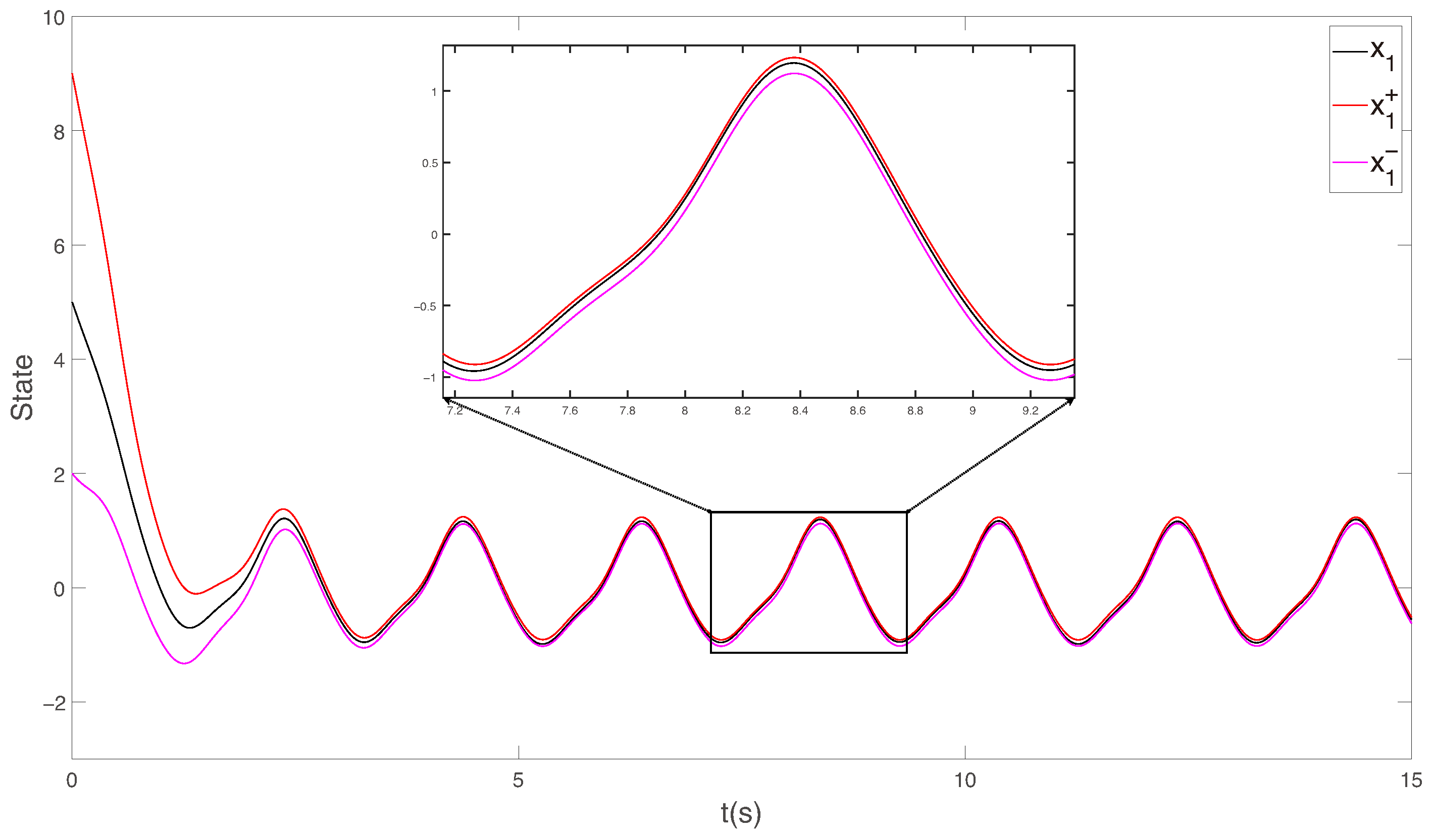
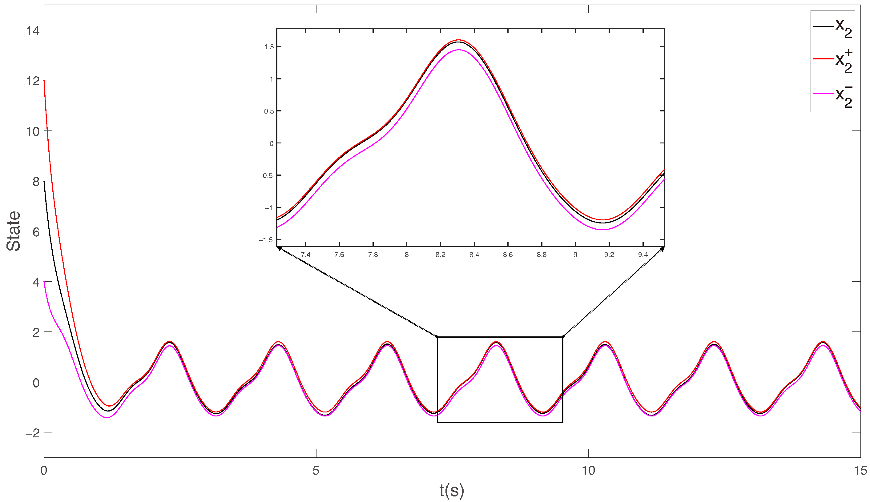
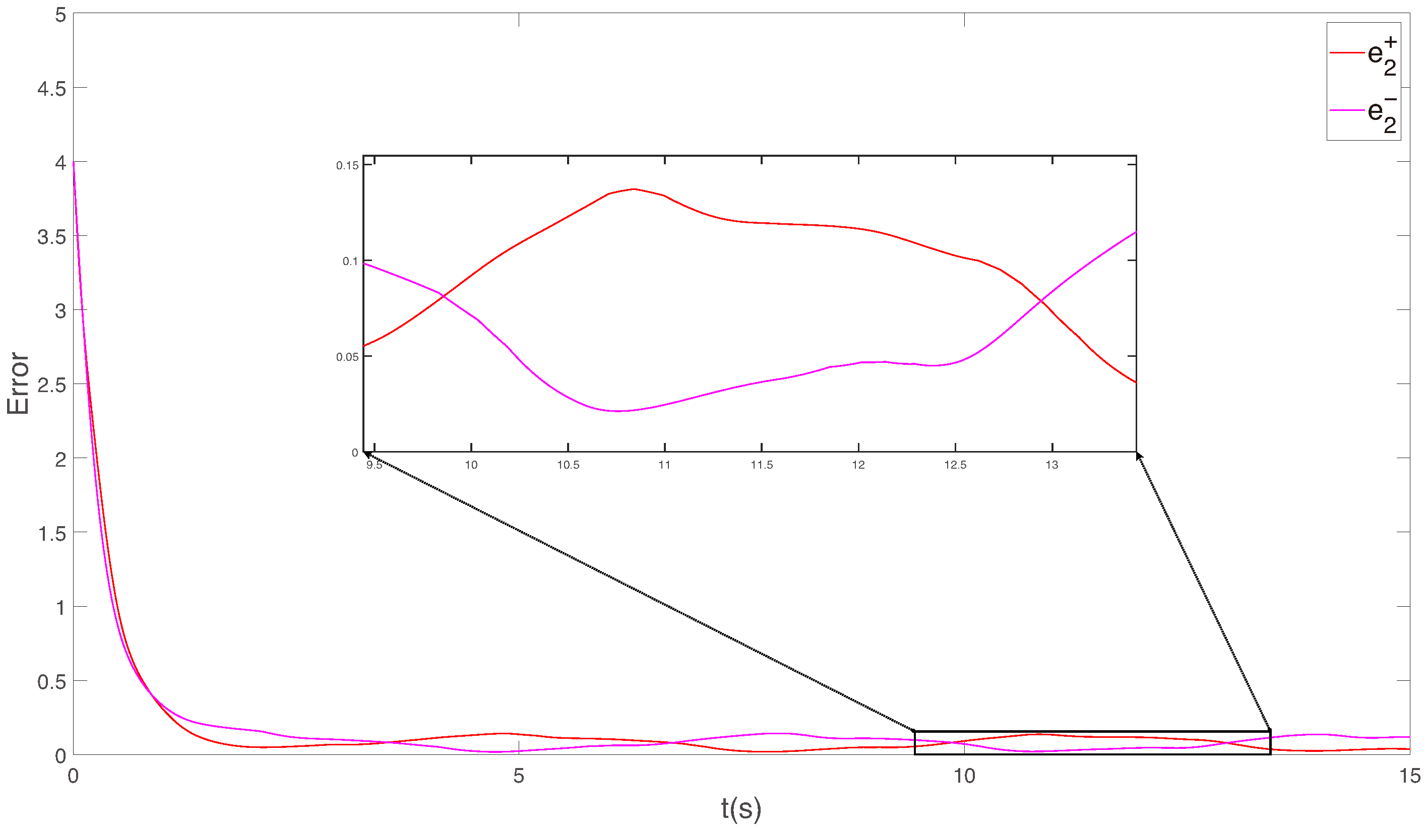
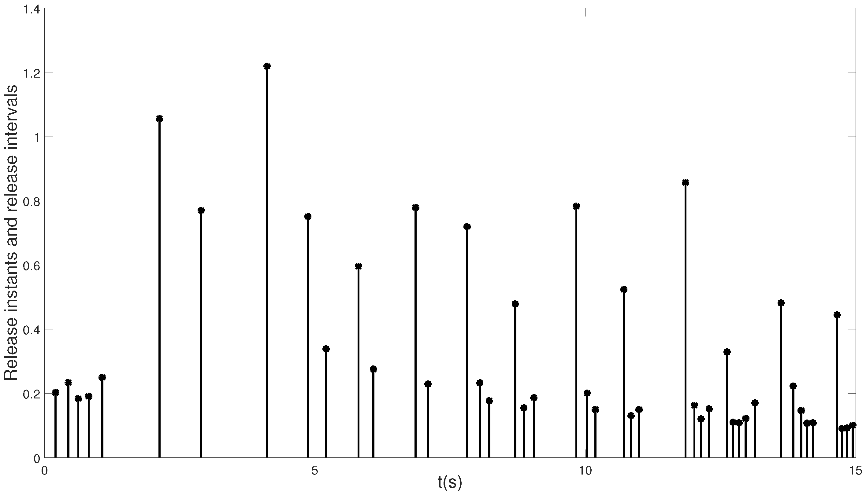
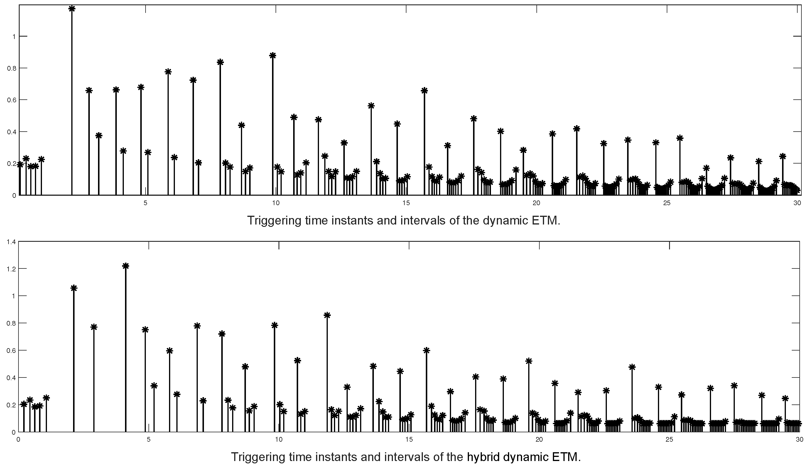
4. Numerical Simulation

Consider a nonlinear cyber–physical system with the following parameters:

$$A=\left[\begin{array}{cc}-3& 1\\ 0& -4\end{array}\right],B=\left[\begin{array}{c}1\\ 2\end{array}\right],$$

$$C=\left[\begin{array}{cc}0.3& 0\end{array}\right],D=\left[\begin{array}{c}0.01\\ 1\end{array}\right].$$

Let the nonlinear function $F\left(x\left(t\right)\right)=\left[\begin{array}{c}0.5sin{x}_1\left(t\right)\\ 0.5sin{x}_2\left(t\right)\end{array}\right]$ and the disturbance $d\left(t\right)=0.5sin\left(t\right)$. According to Lemma 3, we obtain the matrix $\varrho$ in Equation (25) as

$$\varrho =\left[\begin{array}{cccc}2& 0& 1& 0\\ 0& 2& 0& 1\\ 2& 0& 1& 0\\ 0& 2& 0& 1\end{array}\right],$$

with $d^{+}\left(t\right)=0.5$ and $d^{-}\left(t\right)=-0.5$.

Before simulation, initial values of the system need to be assigned, $x_1\left(0\right)=5$, $x_2\left(0\right)=8$. And the initial values of the designed interval observer satisfy $x_1^{+}\left(0\right)=9$, $x_1^{-}\left(0\right)=2$, $x_2^{+}\left(0\right)=12$ and $x_2^{+}\left(0\right)=4$. Additionally, the input is given by $u\left(t\right)=sin\left(2\pi t\right)+3cos\left(\pi t\right)+0.5sin\left(3\pi t\right)$. Other parameters are provided as follows: $\eta \left(0\right)=0.1$, $\alpha =0.5$, $\beta =0.01$, $c_0=20$, $c_1=0.5$, $c_2=20$, $\varphi \left(0\right)=20$, $\gamma =0.8$, $\lambda =0.01$, $k=1$, and $v_i=0.5$.

By solving problem (21), the minimum triggering interval ${\tau }_M=0.0754$, so we take $t_{ETI}^{min}=0.0604$. According to Theorem 2, the gain matrix and the event-triggered weighting matrix are obtained as

$$L=\left[\begin{array}{c}-0.1\\ -0.2\end{array}\right],P=\left[\begin{array}{cc}16.1082& 1.8671\\ 1.8671& 14.7024\end{array}\right],\overline{P}=0.8239,Q=143.6600.$$

Figure 3 and Figure 4 display the interval estimation of the state trajectories $x_1\left(t\right)$ and $x_2\left(t\right)$, respectively. Figure 5 and Figure 6 illustrate the accuracy of the state estimation, which demonstrates the effectiveness and correctness of the designed IO. Additionally, Figure 7 represents the event-triggered intervals and the triggering instants, indicating that all event-triggered intervals are greater than the pre-designed $t_{ETI}^{min}$, thus saving system resources. And

Table 1. Trigger times for different $t_{ETI}^{min}$.

$t_{ETI}^{min}$	0.0504	0.0604	0.1346
Number of triggers (30 s)	193	183	143
The utilization rate of system resources	0.643%	0.610%	0.477%

presents the number of triggering events for different values of $t_{ETI}^{min}$. It can be observed that, while ensuring the estimation performance, as the pre-designed $t_{ETI}^{min}$ increases, the number of triggering events gradually decreases, which also implies a reduction in the consumption of system resources.

Additionally, we have conducted a comparison between the hybrid dynamic ETM designed in this paper and the dynamic ETM in [33], as illustrated in Figure 8. It is evident that the hybrid dynamic ETM has a distinct MIET, which prevents the system’s operational failures caused by the excessively short triggering intervals resulting from the dynamic ETM shown in Figure 8, which may not be achievable with the required precision in practical hardware applications. Moreover,

Table 2. Trigger times for different event triggering mechanisms.

Different ETM	Hybrid Dynamic ETM of This Paper	Dynamic ETM of [33]
Number of triggers	183	223

presents the number of triggers for both event-triggering mechanisms. The hybrid dynamic ETM designed in this paper results in fewer triggers, leading to a lower utilization rate of system resources, thus achieving resource conservation.

5. Conclusions

This paper investigates the state estimation problem of CPSs under a hybrid dynamic ETM. The hybrid dynamic ETM studied allows for controlling the number of updates and information transmissions through a pre-designed MIET control, thereby conserving system resources. It also avoids the infinite triggering failure of the trigger in practical engineering due to hardware limitations, providing broad possibilities for practical applications. Furthermore, for nonlinear CPSs subject to disturbances, we addressed the nonlinear conditions through the Lipschitz condition and designed a novel HDETIO using a positive system approach. The stability and robustness of the designed interval observer were analyzed through Lyapunov stability analysis, solving the state interval estimation problem of CPSs. Future research will concentrate on enhancing the estimation accuracy and relaxing the limitations of this approach, as well as applying the designed HDETIO to CPSs subjected to attacks or various types of disturbances.

References

1. Pasqualetti, F.; Dörfler, F.; Bullo, F. Attack detection and identification in cyber-physical systems. IEEE Trans. Autom. Control 2013, 58, 2715–2729. [Google Scholar] [CrossRef]
2. Yu, X.; Xue, Y. Smart grids: A cyber-physical systems perspective. Proc. IEEE 2016, 104, 1058–1070. [Google Scholar] [CrossRef]
3. Sampigethaya, K.; Poovendran, R. Aviation cyber–physical systems: Foundations for future aircraft and air transport. Proc. IEEE 2013, 101, 1834–1855. [Google Scholar] [CrossRef]
4. Cai, S.; Lau, V.K.N. A stability analysis framework for multiantenna multisensor cyber-physical systems with rank-deficient measurement matrices. IEEE Trans. Control Netw. Syst. 2020, 7, 30–41. [Google Scholar] [CrossRef]
5. Lv, C.; Liu, Y.; Hu, X.; Guo, H.; Cao, D.; Wang, F.Y. Simultaneous observation of hybrid states for cyber-physical systems: A case study of electric vehicle powertrain. IEEE T. Cybern. 2018, 48, 2357–2367. [Google Scholar] [CrossRef]
6. Hu, L.; Wang, Z.; Han, Q.L.; Liu, X. State estimation under false data injection attacks: Security analysis and system protection. Automatica. 2018, 87, 176–183. [Google Scholar] [CrossRef]
7. Ao, W.; Song, Y.; Wen, C.; Lai, J. Finite time attack detection and supervised secure state estimation for CPSs with malicious adversaries. Inf. Sci. 2018, 451–452, 67–82. [Google Scholar] [CrossRef]
8. Gouzé, J.; Rapaport, A.; Hadj-Sadok, M. Interval observers for uncertain biological systems. Ecol. Model. 2000, 133, 45–56. [Google Scholar] [CrossRef]
9. Ethabet, H.; Rabehi, D.; Efimov, D.; Raïssi, T. Interval estimation for continuous-time switched linear systems. Automatica 2018, 90, 230–238. [Google Scholar] [CrossRef]
10. Marouani, G.; Dinh, T.N.; Raïssi, T.; Wang, X.; Messaoud, H. Unknown input interval observers for discrete-time linear switched systems. Eur. J. Control 2021, 59, 165–174. [Google Scholar] [CrossRef]
11. Ogura, T.; Hosoe, Y.; Hagiwara, T. Robust H2 analysis of discrete-time linear systems characterized by random polytopes and time-varying parameters. IFAC-Pap. OnLine 2023, 56, 10402–10407. [Google Scholar] [CrossRef]
12. Zhang, W.; Wang, Z.; Raïssi, T.; Shen, Y. Ellipsoid-based interval estimation for Lipschitz nonlinear systems. IEEE Trans. Autom. Control 2022, 67, 6802–6809. [Google Scholar] [CrossRef]
13. Zhu, F.; Tang, Y.; Wang, Z. Interval-observer-based fault detection and isolation design for T-S fuzzy system based on zonotope analysis. IEEE Trans. Fuzzy Syst. 2022, 30, 945–955. [Google Scholar] [CrossRef]
14. Raissi, T.; Efimov, D.; Zolghadri, A. Interval state estimation for a class of nonlinear systems. IEEE Trans. Autom. Control 2012, 57, 260–265. [Google Scholar] [CrossRef]
15. Huang, J.; Che, H.; Raïssi, T.; Wang, Z. Functional interval observer for discrete-time switched descriptor systems. IEEE Trans. Autom. Control 2022, 67, 2497–2504. [Google Scholar] [CrossRef]
16. Fan, J.; Huang, J.; Zhao, X. Improved interval estimation method for cyber-physical systems under stealthy deception attacks. IEEE Trans. Signal Inf. Proc. Netw. 2022, 8, 1–11. [Google Scholar] [CrossRef]
17. Heemels, W.P.M.H.; Donkers, M.C.F.; Teel, A.R. Periodic event-triggered control for linear systems. IEEE Trans. Autom. Control 2013, 58, 847–861. [Google Scholar] [CrossRef]
18. Shi, D.; Chen, T.; Shi, L. Event-triggered maximum likely-hood state estimation. Automatica 2014, 50, 247–254. [Google Scholar] [CrossRef]
19. Zhang, Q.; Yan, H.; Zhang, H.; Chen, S.; Wang, M. H∞ control of singular system based on stochastic cyber-attacks and dynamic event-triggered mechanism. IEEE Trans. Syst. Man Cybern. Syst. 2021, 51, 7510–7516. [Google Scholar] [CrossRef]
20. Wu, C.; Zhao, X.; Wang, B.; Xing, W.; Liu, L.; Wang, X. Model-based dynamic event-triggered control for cyber-physical systems subject to dynamic quantization and DoS attacks. IEEE Trans. Netw. Sci. Eng. 2022, 9, 2406–2417. [Google Scholar] [CrossRef]
21. Ding, L.; Han, Q.L.; Ge, X.; Zhang, X.M. An overview of recent advances in event-triggered consensus of multiagent systems. IEEE Trans. Cybern. 2018, 48, 1110–1123. [Google Scholar] [CrossRef]
22. Huong, D.C.; Huynh, V.T.; Trinh, H. Dynamic event-triggered state observers for a class of nonlinear systems with time delays and disturbances. IEEE Trans. Circuits Syst. II-Express Briefs. 2020, 67, 3457–3461. [Google Scholar] [CrossRef]
23. Issa, S.A.; Kar, I. Event-triggered adaptive backstepping control of nonlinear uncertain systems with input delay. IFAC-Pap. OnLine 2022, 55, 667–672. [Google Scholar] [CrossRef]
24. Issa, S.A.; Kar, I.N. Design and implementation of event-triggered adaptive controller for commercial mobile robots subject to input delays and limited communications. Control Eng. Pract. 2021, 114, 104865. [Google Scholar] [CrossRef]
25. Cheng, B.; Li, Z. Fully distributed event-triggered protocols for linear multiagent networks. IEEE Trans. Autom. Control 2019, 64, 1655–1662. [Google Scholar] [CrossRef]
26. Cheng, B.; Lv, Y.; Li, Z. Distributed adaptive event-triggered consensus with discrete control updating. In Proceedings of the 2020 59th IEEE Conference on Decision and Control (CDC), Jeju, Republic of Korea, 14–18 December 2020; pp. 2793–2798. [Google Scholar] [CrossRef]
27. Zhao, G.; Hua, C.; Guan, X. A hybrid event-triggered approach to consensus of multiagent systems with disturbances. IEEE Trans. Control Netw. Syst. 2020, 7, 1259–1271. [Google Scholar] [CrossRef]
28. Zhao, G.; Wang, Y.; Fu, X. Hybrid event-triggered consensus tracking of multi-agent systems with discrete control update. IEEE Trans. Circuits Syst. II-Express Briefs. 2022, 69, 2206–2210. [Google Scholar] [CrossRef]
29. Zhang, H.; Huang, J.; He, S. Fractional-order interval observer for multiagent nonlinear systems. Fractal Fract. 2022, 6, 355. [Google Scholar] [CrossRef]
30. Efimov, D.; Raissi, T.; Zolghadri, A. Control of nonlinear and LPV systems: Interval observer-based framework. IEEE Trans. Autom. Control 2013, 58, 773–778. [Google Scholar] [CrossRef]
31. Girard, A. Dynamic triggering mechanisms for event-triggered control. IEEE Trans. Autom. Control 2014, 60, 1992–1997. [Google Scholar] [CrossRef]
32. Hou, Q.; Dong, J. Robust adaptive event-triggered fault-tolerant consensus control of multiagent systems with a positive minimum interevent time. IEEE Trans. Syst. Man Cybern. Syst. 2023, 53, 4003–4014. [Google Scholar] [CrossRef]
33. Wang, X.; Park, J.H. State-based dynamic event-triggered observer for one-sided Lipschitz nonlinear systems with disturbances. IEEE Trans. Circuits Syst. II-Express Briefs. 2022, 69, 2326–2330. [Google Scholar] [CrossRef]
Figure 1. The IO structure with HDETM.
Fractalfract 09 00086 g001
Figure 2. Triggering time instants and intervals.
Fractalfract 09 00086 g002
Figure 3. The state x 1 and its interval estimation.
Fractalfract 09 00086 g003
Figure 4. The state x 2 and its interval estimation.
Fractalfract 09 00086 g004
Figure 5. The estimation error of x 1 .
Fractalfract 09 00086 g005
Figure 6. The estimation error of x 2 .
Fractalfract 09 00086 g006
Figure 7. Triggering instants and triggering intervals.
Fractalfract 09 00086 g007
Figure 8. Triggering instants and triggering intervals of hybrid dynamic ETM and dynamic ETM [33] under 30 s.
Fractalfract 09 00086 g008