Article

An Improved Numerical Scheme for 2D Nonlinear Time-Dependent Partial Integro-Differential Equations with Multi-Term Fractional Integral Items

1
School of Mathematics and Statistics, Guizhou University, Guiyang 550025, China
2
School of Mathematics and Physics, Anhui Jianzhu University, Hefei 230601, China
*
Author to whom correspondence should be addressed.
Fractal Fract. 2025, 9(3), 167; https://doi.org/10.3390/fractalfract9030167
Submission received: 24 January 2025 / Revised: 1 March 2025 / Accepted: 3 March 2025 / Published: 11 March 2025

Abstract

:
This paper is dedicated to investigating a highly accurate numerical solution for a class of 2D nonlinear time-dependent partial integro-differential equations with multi-term fractional integral items. These integrals are weakly singular with respect to time, which are handled using the product integration rule on graded meshes to compensate for the influence generated by the initial weak singular nature of the exact solution. The temporal derivative is approximated by a generalized Crank–Nicolson difference scheme, while the nonlinear term is approximated by a linearized method. Furthermore, the stability and convergence of the derived time semi-discretization scheme are strictly proved by revising the finite discrete parameters. Meanwhile, the differential matrices of the spatial high-order derivatives based on barycentric rational interpolation are utilized to obtain the fully discrete scheme. Finally, the effectiveness and reliability of the proposed method are validated by means of several numerical experiments.

1. Introduction

Fractional evolution equations can characterize the physical and engineering phenomena by simulating memory effects and non-locality [1,2,3,4,5]. The nonlinear form of equations of this type provides a more accurate description of certain reality phenomena in comparison with the linear form [6,7,8,9]. Many scholars have attempted to seek numerical solutions since analytical solutions of these equations are mostly challenging to obtain [10,11,12,13]. In this paper, 2D nonlinear time-dependent Volterra partial integro-differential equations with multi-term weakly singular kernels are considered as follows:
t u ( x , y , t ) μ t Δ u ( x , y , t ) = I ( α 1 ) u x x ( x , y , t ) + I ( α 2 ) u y y ( x , y , t ) + G ( u ) + f ( x , y , t ) , ( x , y ) Ω , t ( 0 , T ] ,
with the initial condition
u ( x , y , 0 ) = u 0 ( x , y ) , ( x , y ) Ω ¯ = Ω Ω ,
and the Dirichlet boundary condition
u ( x , y , t ) = u b ( x , y , t ) , ( x , y ) Ω , t [ 0 , T ] ,
where μ > 0 , Δ represents the 2D Laplacian operator, the third-order spatiotemporal mixed partial derivative introduces the viscosity effect, and I ( α ) is the α -order Riemann–Liouville fractional integral operator defined as follows:
I ( α ) g ( · , t ) = 1 Γ ( α ) 0 t ( t s ) α 1 g ( · , s ) d s , 0 < α < 1 ,
which is weakly singular concerning time, and Γ ( · ) is the Gamma function. If the integral items in Equation (1) are removed, then Equation (1) becomes a classical Sobolev-type equation, which has been the subject of study by many researchers [14,15]. Ω R 2 is an open and bounded rectangular region with the corresponding boundary Ω , the nonhomogeneous terms f ( x , y , t ) , u 0 ( x , y ) , and u b ( x , y , t ) are all known functions, and the nonlinear term G ( u ) C 2 ( R ) is Lipschitz continuous with the Lipschitz constant L > 0 , that is,
| G ( u ) G ( u ˜ ) | L | u u ˜ | .
Particularly, Equation (1) is linear when G ( u ) : = u or 0. The linear situation of Equation (1) arises from many models for heat flow in a rectangular, orthotropic material with memory, which has been investigated by some researchers [16,17,18]. Recently, significant research has been carried out regarding problems analogous to (1). In [19], Chen et al. proposed a BDF2 compact difference scheme to solve a class of α -order Riemann–Liouville fractional integral equations and achieved the temporal convergence rate with 1 + α . In [20], Qiao et al. investigated a class of integro-differential equations with multi-term weakly singular kernels using the BDF2 ADI orthogonal spline collocation scheme, resulting in a convergence rate with min { 1 + α 1 , 1 + α 2 } . Due to the insufficient smoothness of solution close to initial point, these methods do not succeed in attaining the expected second-order convergence, though their convergence orders are generally higher than first-order. The use of graded meshes with smaller time steps near t = 0 can handle the initial weak singularity of the solution [21]. Several other studies related to graded meshes are outlined in [22,23,24,25]. The product integration rule based on the piecewise linear interpolation is a second-order quadrature formula, which is commonly used to approximate integrals [26]. Since piecewise linear interpolation imposes no special requirements on the nodes, the graded meshes can be applied to the product integration rule. In [27], a BDF2 ADI OSC scheme on graded meshes was proposed to solve the 3D nonlinear fractional evolution equation, whose integral term is approximated by the product integration rule. Wu et al. in [28] constructed a second-order CN difference method on graded meshes to solve the fourth-order evolution equation with multi-term integrals. Their theoretical analyses referred to Lemma 4.2.3 in [19]; it is shown that the product integration rule achieves second-order convergence for suitable grading exponents. In this paper, we focus on resolving a general 2D nonlinear case of Equation (1) and handle the weak singularities of the solution at the initial moment based on the graded meshes. The smoothness assumptions of the solution follow the reference [29], that is,
| u ( · , t ) | c t α + 1 , | u t ( · , t ) | c t α , t [ 0 , T ] , | u t t ( · , t ) | c t α 1 , t ( 0 , T ] ,
where α = max { α 1 , α 2 } , c refers to a generic positive constant, which is not necessarily uniform in distinct circumstances in this paper. Additionally, we perform a dimensional analysis on Equation (1). Suppose the dimensions of u, the time variable t, and the spatial variables x and y are represented by [ U ] , [ T ] , and [ L ] , respectively, then
u t [ U ] [ T ] , Δ u t [ U ] [ T ] · [ L ] 2 , I ( α 1 ) u x x [ U ] · [ T ] α 1 [ L ] 2 , I ( α 2 ) u y y [ U ] · [ T ] α 2 [ L ] 2 .
To ensure dimensional homogeneity, we assign the dimensions of the coefficients of the second, third, and fourth terms in Equation (1) as [ L ] 2 , [ L ] 2 [ T ] 1 + α 1 , and [ L ] 2 [ T ] 1 + α 2 , respectively.
The non-negativity theorem presented by Lopez-Marcos in [29] is a forceful tool to testify to the stability and convergence of numerical approaches for fractional evolution equations; some specific applications can be found in [30,31,32]. In [33], Tang approximated the 1 / 2 -order Riemann–Liouville fractional integral operator by the product integration rule and stated that the former n 1 terms of the product integration rule satisfy the non-negativity theorem, while the n-th term does not. Furthermore, Chen et al. extended this result and proved that the first n 1 terms of the product integration rule consistently satisfy the non-negativity theorem for any α and graded meshes in [34]. However, numerical results demonstrate that it is a common phenomenon for the failure of the n-th term of the product integration method to satisfy the non-negativity theorem, which makes the proof complicated or unrigorous. In this paper, the stable and convergent properties of the numerical method are proved by modifying the n-th term and employing the discrete Gronwall lemma without affecting the whole algorithm.
The principal objective of this paper is to formulate a highly accurate numerical approach for solving Equation (1). The whole structure is outlined as follows. In Section 2, some preparations are made. In Section 3, a time semi-discretization scheme results via a generalized Crank–Nicolson difference scheme, a product integration rule, and a linearized method. Sequentially, stability and convergence of the temporal semi-discrete scheme are discussed through the energy method. In Section 4, barycentric rational interpolation is employed to deduce the fully discrete scheme. In Section 5, some numerical results are displayed to support the theoretical consequences. This paper ends with a brief conclusion in Section 6.

2. Preparations

2.1. Product Integration Rule

In this part, some preparations are made for approximating the integral and differential terms involving the time variable in Equation (1).
With the aim of discretizing the fractional integral terms related to time in Equation (1), we first devote ourselves to estimating the following Riemann–Liouville fractional integral:
I ( α ) g ( t ) = 1 Γ ( α ) 0 t ( t s ) α 1 g ( s ) d s , t ( 0 , T ] ,
with 0 < α < 1 . For N N + , we partition [ 0 , T ] into N subintervals with the graded mesh
t n = T n N r , n = 0 , 1 , , N ,
where r is referred to as a grading exponent, we always set r 1 in this paper. The temporal step size is
τ n = t n t n 1 = τ 1 [ n r ( n 1 ) r ] , n = 1 , 2 , , N ,
obviously, τ 1 = T / N r . It’s clear that
τ 1 = min 1 n N { τ n } , τ : = τ N = max 1 n N { τ n } .
By taking the quotient of τ n and τ n 1 , one can readily confirm that
τ n 1 τ n ( 2 r 1 ) τ n 1 .
Let g n = g ( t n ) for any mesh nodes t n , then the piecewise linear interpolation of g ( t ) on the graded mesh in (6) can be defined by
P g ( t ) = t t n 1 τ n g n + t n t τ n g n 1 , t [ t n 1 , t n ] ,
for n = 1 , 2 , , N . Based on (9), the approximation of I ( α ) g ( t n ) is
Q n ( α ) ( g ) = 1 Γ ( α ) 0 t n ( t n s ) α 1 P g ( s ) d s = τ 1 α Γ ( α + 2 ) p = 0 n b n , p ( α ) g p ,
where
b n , p ( α ) = ( n r 1 ) α + 1 n r α ( n r α 1 ) , p = 0 , φ n , p ( r , α ) φ n , p + 1 ( r , α ) , p = 1 , 2 , , n 1 , n r ( n 1 ) r ] α , p = n ,
with φ n , p ( r , α ) = [ n r ( p 1 ) r ] α + 1 ( n r p r ) α + 1 p r ( p 1 ) r . The numerical quadrature rule (10) is called product integration rule in [26], there I ( α ) g ( t n ) Q n ( α ) ( g ) . Correspondingly, the error is defined as follows:
E ( α ) ( g ) ( t n ) = I ( α ) g ( t n ) Q n ( α ) ( g ) = I ( α ) ( g ( t n ) P g ( t n ) ) .
Before estimating | E ( α ) ( g ) ( t n ) | , we first give an estimation of the interpolation error | g ( t ) P g ( t ) | .
Lemma 1.
Assume that g ( t ) C 1 [ 0 , T ] C 2 ( 0 , T ] , | g ( t ) | c t α for t [ 0 , T ] and | g ( t ) | c t α 1 for t ( 0 , T ] , where 0 < α < 1 . If P g ( t ) is defined in (9) and r 2 α + 1 , then
| g ( t ) P g ( t ) | c N 2 c τ 2 .
Proof. 
For t 0 t t 1 , we give the following equivalent representation as
g ( t ) P g ( t ) = t t 0 τ 1 ( g ( t ) g 1 ) + t 1 t τ 1 ( g ( t ) g 0 ) .
Then, according to the Lagrange mean value theorem, there exist ξ 0 ( t 0 , t ) and ξ 1 ( t , t 1 ) such that
| g ( t ) P g ( t ) | = | t t 0 τ 1 g ( ξ 1 ) ( t t 1 ) + t 1 t τ 1 g ( ξ 0 ) ( t t 0 ) | | ( t t 0 ) ( t t 1 ) τ 1 | · | g ( ξ 1 ) + g ( ξ 0 ) | 1 2 τ 1 max t 0 t t 1 | g ( t ) | .
Since | g ( t ) | c t α and r 2 α + 1 , then
| g ( t ) P g ( t ) | c τ 1 α + 1 = c T N r α + 1 c T α + 1 N 2 c τ 2 .
Next, for t n 1 t t n with 2 n N , similarly, we also give an equivalent expression as
g ( t ) P g ( t ) = t t n 1 τ n ( g ( t ) g n ) + t n t τ n ( g ( t ) g n 1 ) .
Further, using the Lagrange remainder term of the Taylor series and | g ( t ) | c t α 1 , there is
| g ( t ) P g ( t ) | = | ( t t n 1 ) ( t t n ) 2 τ n | · | g ( ξ n ) ( t n t ) + g ( ξ n 1 ) ( t t n 1 ) | 1 8 τ n 2 max t n 1 t t n | g ( t ) | c τ n 2 t n 1 α 1 ,
where ξ n 1 ( t n 1 , t ) , ξ n ( t , t n ) . Based on the graded mesh in (6) and the time step in (7), there are
τ n = T · n r ( n 1 ) r N r = r N · T η N r 1 r N · T n N r ( 1 1 r ) = r N T 1 r t n 1 1 r , t n 1 1 = t n 1 t n t n 1 = t n 1 n n 1 r 2 r t n 1 , n = 2 , 3 , , N ,
where η ( n 1 , n ) . We now return (13) and derive that
| g ( t ) P g ( t ) | c r N T 1 r t n 1 1 r 2 ( 2 r t n 1 ) ( 1 α ) = c 2 r ( 1 α ) r 2 N 2 T 2 r t n 2 ( 1 1 r ) + α 1 .
For r 2 α + 1 , noting that the exponent 2 ( 1 1 r ) + α 1 0 , thus
| g ( t ) P g ( t ) | c N 2 c τ 2 .
The proof is complete. □
On the basis of Lemma 1, the following error estimation is straightforward.
Lemma 2.
On the assumption of g ( t ) in Lemma 1, I ( α ) g ( t n ) and Q n ( α ) ( g ) is defined in (5) and (10), respectively. If r 2 α + 1 , then an error estimation of the product integration rule is
| I ( α ) g ( t n ) Q n ( α ) ( g ) | c τ 2 .
Proof. 
A direct result is derived from Lemma 1 that
| I ( α ) g ( t n ) Q n ( α ) ( g ) | = | I ( α ) ( g ( t n ) P g ( t n ) ) | | c τ 2 1 Γ ( α ) 0 t n ( t n s ) α 1 d s | c τ 2 .
In order to achieve the discretization of the differential term involving time in Equation (1), a generalized Crank–Nicolson (GCN) difference scheme is considered. According to the Taylor expansion with integral remainder, the GCN difference scheme is as follows:
Lemma 3
[35]. Let v C 3 [ t n 1 , t n ] for n = 1 , , N , then
v ( t n ) + v ( t n 1 ) 2 v ( t n ) v ( t n 1 ) τ n = τ n 2 16 0 1 v ( 3 ) t n 1 2 + s τ n 2 + v ( 3 ) t n 1 2 s τ n 2 ( 1 s 2 ) d s ,
where τ n is defined in Equation (7), and t n 1 2 = t n 1 + 1 2 τ n .

2.2. Barycentric Form of Floater–Hormann Rational Interpolation

There, we make preparations for accomplishing the discretizations of spatial derivatives in Equation (1); a high-order linear barycentric rational interpolation (BRI) based on Floater–Hormann interpolation is considered. Also, the related differential matrices will be derived.
Let { x j } j = 0 M be given distinct points on interval [ a , b ] . From [36], the barycentric form of Floater–Hormann interpolants of v ( x ) regarding x j is
R v ( x ) = j = 0 M L j ( x ) v j , L j ( x ) = β j x x j / j = 0 M β j x x j , β j = i J j ( 1 ) i k = i , k j i + d 1 x j x k ,
where v j = v ( x j ) , R v ( x ) is also often referred to as BRI with satisfying interpolation conditions. R v ( x j ) = v ( x j ) , L j ( x ) are BRI basis functions, β j are BRI weights, d is a BRI parameter with 0 d M , the index J j = { i { 0 , 1 , , M } : j d i j } . It was known in [36] that for v C d + 2 [ a , b ] , there is
v R v c h d + 1 ,
where h is the maximum mesh size.
Since R v ( x ) is a linear combination of L j ( x ) , the derivatives of R v ( x ) can be transformed into a linear combination of the derivatives of L j ( x ) . Therefore, the m-order derivatives of R v ( x ) can be calculated by
R v ( m ) ( x ) = j = 0 M L j ( m ) ( x ) v j ,
where m N . Then, the function values of R v ( m ) ( x ) at the point { x i } i = 0 M are
R v ( m ) ( x i ) = j = 0 M L j ( m ) ( x i ) v j = j = 0 M D i , j ( m ) v j ,
where D i , j ( m ) = L j ( m ) ( x i ) . From [37], the computation formulas of D i , j ( m ) is provided by
D i , j ( 1 ) = L j ( x i ) = β j / β i x i x j , i j , i j D i , j ( 1 ) , i = j ,
D i , j ( m ) = L j ( m ) ( x i ) = m D i , i ( m 1 ) D i , j ( 1 ) D i , j ( m 1 ) x i x j , i j , i j D i , j ( m ) , i = j .
The coming lemma provides an error estimation of the second-order derivative of BRI.
Lemma 4
[38]. Let 1 d M ; if v ( x ) C d + 3 [ a , b ] and R v ( x ) is the BRI defined in (15). Then for large enough M, there is
v R v c h d 1 .
The BRI is a class of node-type interpolation, so it can be naturally extended to 2D interpolation on a rectangular domain by utilizing tensor product nodes. Let { ( x j 1 , y j 2 ) | j 1 = 0 , 1 , , M 1 , j 2 = 0 , 1 , , M 2 } be distinct grid points on Ω , u j 1 , j 2 = u ( x j 1 , y j 2 ) . From [36,39], the 2D-BRI of u ( x , y ) associated with ( x j 1 , y j 2 ) is defined by
R u ( x , y ) = j 1 = 0 M 1 j 2 = 0 M 2 L j 1 ( x ) L j 2 ( y ) u j 1 , j 2 ,
which satisfies the interpolation conditions R u ( x j 1 , y j 2 ) = u j 1 , j 2 , L j 1 ( x ) and L j 2 ( y ) are the BRI basis functions along x and y directions, respectively.
It is analogous to the deduction of derivative function (17). For m 1 , m 2 N , since R u ( x , y ) is linear with respect to u j 1 j 2 , the ( m 1 + m 2 ) -order partial derivatives of u ( x , y ) can be estimated as follows:
R u ( m 1 , m 2 ) ( x , y ) : = m 1 + m 2 R u ( x , y ) x m 1 y m 2 = j 1 = 0 M 1 j 2 = 0 M 2 L j 1 ( m 1 ) ( x ) L j 2 ( m 2 ) ( y ) u j 1 , j 2 .
Then, the values of R u ( m 1 , m 2 ) ( x , y ) at { ( x i 1 , y i 2 ) | i 1 = 0 , 1 , , M 1 ; i 2 = 0 , 1 , , M 2 } are
R u ( m 1 , m 2 ) ( x i 1 , y i 2 ) : = m 1 + m 2 R u ( x i 1 , y i 2 ) x m 1 y m 2 = j 1 = 0 M 1 j 2 = 0 M 2 L j 1 ( m 1 ) ( x i 1 ) L j 2 ( m 2 ) ( y i 2 ) u j 1 , j 2 = j 1 = 0 M 1 j 2 = 0 M 2 C i 1 , j 1 ( m 1 ) D i 2 , j 2 ( m 2 ) u j 1 , j 2 ,
where C i 1 , j 1 ( m 1 ) = L j 1 ( m 1 ) ( x i 1 ) and D i 2 , j 2 ( m 2 ) = L j 2 ( m 2 ) ( y i 2 ) are the elements of m 1 - and m 2 -order BRI differential matrix, respectively.

2.3. Some Notations

At the conclusion of this section, we put forward the definitions of some function spaces, together with their respective inner products and norms.
The function space L 2 ( Ω ) is denoted by
L 2 ( Ω ) = u : Ω R , Ω u 2 d x d y < ,
where u is a measurable function and d x d y is the Lebesgue measure. The inner product and corresponding norm in the function space L 2 ( Ω ) are respectively denoted by
u , v = Ω u v d x d y , u = u , u ,
where u , v L 2 ( Ω ) . Then L 2 ( Ω ) is a Hilbert space in the sence of the above inner product.
Next, we provide the definition of H 1 ( Ω ) space as follows:
H 1 ( Ω ) = u L 2 ( Ω ) , u x , u y L 2 ( Ω ) .
For any u H 1 ( Ω ) , a new norm is defined as follows:
u A = u 2 + μ u 2 .
Obviously, there are
u 2 u A 2 , u 2 1 μ u A 2 .

3. Temporal Discretization

Two main aims are considered in this section. Firstly, the discretization relating to the time variable of (1) is performed in order to construct the temporal semi-discrete scheme. Subsequently, the stability and convergence of the provided approach are discussed.

3.1. Temporal Semi-Discrete Scheme

Based on the foregoing preparations, we now use the Formulas (10) and (14) to obtain the temporal semi-discrete scheme of Equation (1). For briefness, let us introduce some notations:
u n = u ( x , y , t n ) , f n = f ( x , y , t n ) , n = 0 , 1 , , N , D u n = u n u n 1 τ n , f n 1 2 = f n + f n 1 2 , n = 1 , , N .
Now, Equation (1) at the time levels t n and t n 1 are considered leads to
t u n μ t Δ u n = I ( α 1 ) u x x n + I ( α 2 ) u y y n + G ( u n ) + f n , t u n 1 μ t Δ u n 1 = I ( α 1 ) u x x n 1 + I ( α 2 ) u y y n 1 + G ( u n 1 ) + f n 1 .
Then, it yields that
1 2 t u n + u n 1 μ 2 t Δ u n + Δ u n 1 = 1 2 I ( α 1 ) u x x n + I ( α 1 ) u x x n 1 + 1 2 I ( α 2 ) u y y n + I ( α 2 ) u y y n 1 + 1 2 G ( u n ) + G ( u n 1 ) + f n 1 2 .
According to the Taylor expansion with the Lagrange remainder, it holds that
G ( u n ) = G ( u 0 ) + R G 1 , n = 1 , 2 G ( u n 1 ) G ( u n 2 ) + R G n , n 2 .
For n = 1 , there is
R G 1 = | G ( u 1 ) G ( u 0 ) | = | G ( ξ ) ( u 1 u 0 ) | | G ( ξ ) | | u ( ζ ) | τ 1 ,
in which ξ ( u 0 , u 1 ) , ζ ( t 0 , t 1 ) . Similar to the derivation of Equation (12), if r 2 1 + α , R G 1 = O ( τ 2 ) . In addition, for n 2 , R G n = O ( τ 2 ) .
It follows from the formulas (10), (14), and (22) that Equation (21) becomes
D u n μ D Δ u n = τ 1 α 1 Γ ( α 1 + 2 ) p = 0 n ω n , p ( α 1 ) u x x p + τ 1 α 2 Γ ( α 2 + 2 ) p = 0 n ω n , p ( α 2 ) u y y p + G 1 ( u n ) + f n 1 2 + R t n 1 2 ,
where ω n , p ( α i ) = 1 2 b n , p ( α i ) + b n 1 , p ( α i ) for p = 0 , 1 , , n 1 , ω n , n ( α i ) = 1 2 b n , n ( α i ) , i = 1 , 2 , and
G 1 ( u n ) = G ( u 0 ) , n = 1 , 3 2 G ( u n 1 ) 1 2 G ( u n 2 ) , n 2 .
The truncation error term R t n 1 2 is as follows:
R t n 1 2 = R 1 n 1 2 + R G n 1 2 + R 2 n 1 2 , R 1 n 1 2 = 1 2 t ( u n + u n 1 ) D u n + μ 2 t ( Δ u n + Δ u n 1 ) μ D Δ u n , R G n 1 2 = G 1 ( u n ) 1 2 G ( u n ) + G ( u n 1 ) , R 2 n 1 2 = 1 2 E ( α 1 ) ( u x x ) ( t n ) + E ( α 1 ) ( u x x ) ( t n 1 ) + 1 2 E ( α 2 ) ( u y y ) ( t n ) + E ( α 2 ) ( u y y ) ( t n 1 ) .
From Lemmas 2, 3, and Equation (22), it deduces that
| R t n 1 2 | c τ 2 .
We discard R t n 1 2 and substitute u n by U n in Equation (23). Then, the time semi-discretization scheme of Equation (1) can be established as follows:
D U n μ D Δ U n = τ 1 α 1 Γ ( α 1 + 2 ) p = 0 n ω n , p ( α 1 ) U x x p + τ 1 α 2 Γ ( α 2 + 2 ) p = 0 n ω n , p ( α 2 ) U y y p + G 1 ( U n ) + f n 1 2 ,
where U n = U ( x , y , t n ) . Further, the initial condition is U 0 ( x , y ) = u 0 ( x , y ) and the boundary conditions at t n are U n ( x , y ) = u b ( x , y , t n ) for ( x , y ) Ω .

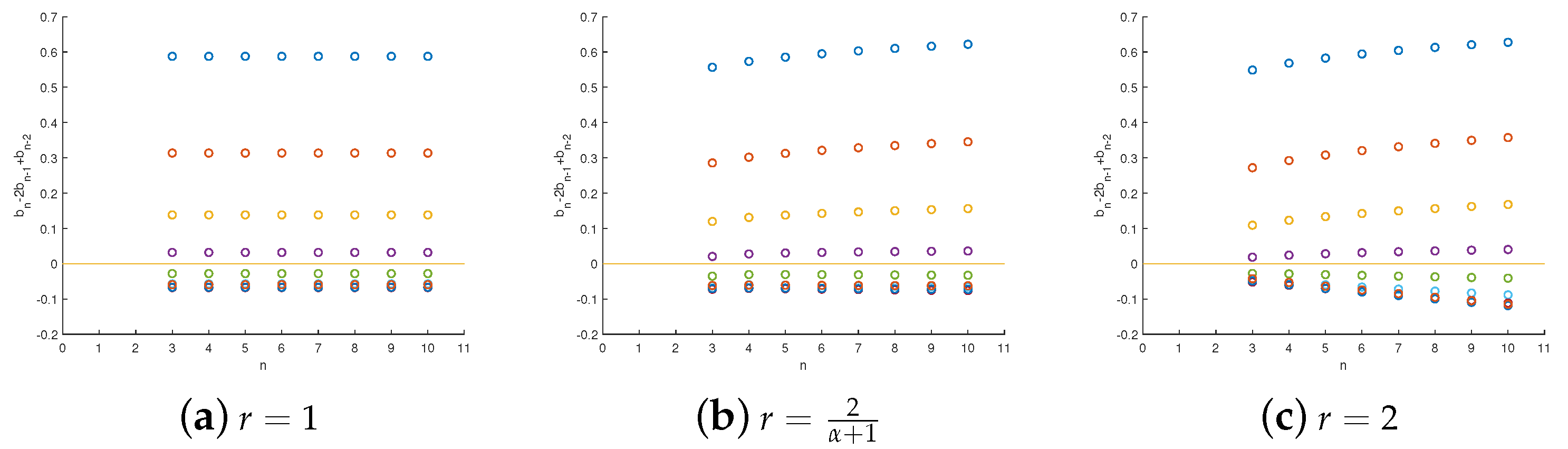
3.2. Stability and Convergence Analysis

Based on the energy method, the stability and convergence of the temporal discrete scheme (26) are discussed in this part. Some definitions, notations, and lemmas are first introduced.
Lemma 5
[29]. Assume that the real number set { a n } n = 0 satisfies
a n 0 , a n a n 1 0 , a n + 1 2 a n + a n 1 0 .
Then for each real vector ( V 1 , , V m ) with m N + , there is
n = 1 m p = 1 n a n p V p V n 0 .
Lemma 6
[33,34]. The denoted sequence b n , p ( α ) p = 1 n 1 in (11) satisfies the following properties:
b n , p ( α ) 0 , b n , p ( α ) b n , p 1 ( α ) 0 , b n , p + 1 ( α ) 2 b n , p ( α ) + b n , p 1 ( α ) 0 .
Proof. 
For simplify, we take the following marks:
I n , p ( α , m ) = 1 Γ ( α ) t p t n ( t n s ) α 1 ( s t p ) m d s = ( t n t p ) α + m m ! Γ ( α + m + 1 ) , m = 0 , 1 .
Thereby,
I n , p 1 ( α , 1 ) I n , p ( α , 1 ) τ p = 1 Γ ( α ) t p t n ( t n s ) α 1 d s + 1 Γ ( α ) τ p t p 1 t p ( t n s ) α 1 ( s t p 1 ) d s .
According to [34], the sequence b n , p ( α ) p = 1 n can also be expressed as
τ 1 α Γ ( α + 2 ) b n , 0 ( α ) = I n , 0 ( α , 0 ) I n , 0 ( α , 1 ) I n , 1 ( α , 1 ) τ 1 , τ 1 α Γ ( α + 2 ) b n , p ( α ) = I n , p 1 ( α , 1 ) I n , p ( α , 1 ) τ p I n , p ( α , 1 ) I n , p + 1 ( α , 1 ) τ p + 1 , p = 1 , 2 , , n 1 , τ 1 α Γ ( α + 2 ) b n , n ( α ) = I n , n 1 ( α , 1 ) τ n .
Then for p = 1 , 2 , , n 1 , there is also
τ 1 α Γ ( α + 2 ) b n , p ( α ) = 1 Γ ( α ) τ p τ p + 1 ( t n t p s ) α 1 1 | s | τ p Z [ τ p , 0 ] + τ p + 1 Z [ 0 , τ p + 1 ] d s ,
where
Z [ c , d ] = 1 , s [ c , d ] , 0 , s [ c , d ] .
It is natural to conclude that b n , p ( α ) 0 for p = 0 , 1 , , n 1 .
Furthermore, the second item of this lemma follows from
d d t p ( t n t p s ) α 1 = ( α 1 ) ( t n t p s ) α 2 > 0 ,
and the third item follows from
d 2 d t p 2 ( t n t p s ) α 1 = ( α 1 ) ( α 2 ) ( t n t p s ) α 3 > 0 ,
for p = 0 , 1 , , n 1 and s [ τ p , τ p + 1 ] . □
It is worth noting that b n , n ( α ) does not always satisfy b n , n ( α ) 2 b n , n 1 ( α ) + b n , n 2 ( α ) 0 or b n , n ( α ) b n , n 1 ( α ) 0 . There exists an example in [33] where b n , n ( α ) 2 b n , n 1 ( α ) + b n , n 2 ( α ) < 0 for α = 0.5 and r = 1 , and this is not an exceptional case. In Figure 1 and Figure 2, let N = 10 ; there are always some points such that b n , n ( α ) 2 b n , n 1 ( α ) + b n , n 2 ( α ) < 0 and b n , n ( α ) b n , n 1 ( α ) < 0 for different α and r. To guarantee the efficiency of Lemma 5, we define
γ n , p ( α ) = 1 2 b 1 , 1 ( α ) + b 2 , 1 ( α ) , n = 2 , p = 2 , 1 2 b 2 , 1 ( α ) + b 3 , 1 ( α ) , n = 3 , p = 2 , b 2 , 1 ( α ) + b 3 , 1 ( α ) + b 2 , 2 ( α ) + b 3 , 2 ( α ) , n = 3 , p = 3 , b n 1 , n 2 ( α ) , n > 3 , p = n 1 , 2 b n 1 , n 2 ( α ) + b n , n 1 ( α ) + b n , n ( α ) , n > 3 , p = n , 0 , others ,
and for any n, p,
ω ¯ n , p ( α ) = ω n , p ( α ) + γ n , p ( α ) .
Clearly, the sequence ω ¯ n , p ( α ) p = 1 n satisfies all the inequalities in (27). Meanwhile,
1 2 Q n ( α ) ( g ) + Q n 1 ( α ) ( g ) = τ 1 α Γ ( α + 2 ) p = 0 n ω n , p ( α ) g p = τ 1 α Γ ( α + 2 ) p = 0 n ω ¯ n , p ( α ) γ n , p ( α ) g p .
Lemma 7
[40]. If the real sequences { z n } n = 0 and { c n } n = 0 are both nonnegative, also
z n b n + m = 0 n 1 c m z m , n 0 ,
where { b n } n = 0 is nonnegative and nondecreasing real sequence. Then the following inequality holds
z n b n exp m = 0 n 1 c m .
Next, two main results of the temporal discrete scheme (26) are given using the energy method. Let u n ( x , y ) represent the exact soluThe symbols of tion of Equation (1) at t = t n and U n ( x , y ) is the solution of Equation (26). We set u n : = u n ( x , y ) and U n : = U n ( x , y ) for weakening disturbance.
Theorem 1.
Assume that U n , U ¯ n H 1 ( Ω ) are the analytical and perturbative solutions of Equation (26), respectively. Then for 0 n N ,
ϵ n C ( T ) ϵ 0 ,
where ϵ n = U n U ¯ n .
Proof. 
According to Equation (26), we can obtain the error equation
D ϵ n μ D Δ ϵ n = τ 1 α 1 Γ ( α 1 + 2 ) p = 0 n ω n , p ( α 1 ) ϵ x x p + τ 1 α 2 Γ ( α 2 + 2 ) p = 0 n ω n , p ( α 2 ) ϵ y y p + G 1 ( U n ) G 1 ( U ¯ n ) .
By taking the inner product of Equation (31) with τ ϵ n and summing n from 1 to m, it yields
τ n = 1 m D ϵ n , ϵ n μ τ n = 1 m D Δ ϵ n , ϵ n = τ 1 α 1 τ Γ ( α 1 + 2 ) n = 1 m p = 0 n ω n , p ( α 1 ) ϵ x x p , ϵ n + τ 1 α 2 τ Γ ( α 2 + 2 ) n = 1 m p = 0 n ω n , p ( α 2 ) ϵ y y p , ϵ n + τ n = 1 m G 1 ( U n ) G 1 ( U ¯ n ) , ϵ n .
Now, each term in Equation (32) can be estimated. For the first term of left hand, we have
τ n = 1 m D ϵ n , ϵ n = τ n = 1 m ϵ n ϵ n 1 τ n , ϵ n + ϵ n 1 2 + τ n = 1 m ϵ n ϵ n 1 τ n , ϵ n ϵ n 1 2 = τ n = 1 m 1 2 τ n ϵ n 2 ϵ n 1 2 + ϵ n ϵ n 1 2 1 2 ( ϵ m 2 ϵ 0 2 ) .
For the second term of left hand, using the Green formula and ϵ n | Ω = 0 , then
μ τ n = 1 m D Δ ϵ n , ϵ n = μ τ n = 1 m D ϵ n , ϵ n = μ τ n = 1 m ϵ n ϵ n 1 τ n , ϵ n + ϵ n 1 2 + μ τ n = 1 m ϵ n ϵ n 1 τ n , ϵ n ϵ n 1 2 = μ τ n = 1 m 1 2 τ n ϵ n 2 ϵ n 1 2 + ϵ n ϵ n 1 2 μ 2 ϵ m 2 ϵ 0 2 .
The integration by parts and Equation (30) are applied to the first term of the right-hand side in Equation (32), then
n = 1 m p = 0 n ω n , p ( α 1 ) ϵ x x p , ϵ n = n = 1 m p = 1 n ω n , p ( α 1 ) ϵ x x p , ϵ n + n = 1 m ω n , 0 ( α 1 ) ϵ x x 0 , ϵ n = n = 1 m p = 1 n ω n , p ( α 1 ) ϵ x p , ϵ x n n = 1 m ω n , 0 ( α 1 ) ϵ x 0 , ϵ x n = n = 1 m p = 1 n ω ¯ n , p ( α 1 ) ϵ x p , ϵ x n n = 1 m ω n , 0 ( α 1 ) ϵ x 0 , ϵ x n + n = 1 m p = 1 n γ n , p ( α ) ϵ x p , ϵ x n .
Based on Lemma 5, the first term of the right-hand side in Equation (35) is non-positive. It follows from the Cauchy–Schwarz inequality and Equation (20) that
ϵ x 0 , ϵ x n ϵ x 0 ϵ x n ϵ 0 ϵ n 1 μ ϵ 0 A ϵ n A , ϵ x p , ϵ x n ϵ x p ϵ x n ϵ p ϵ n 1 μ ϵ p A ϵ n A .
From the above analyses, we can conclude that
n = 1 m p = 0 n ω n , p ( α 1 ) ϵ x x p , ϵ n 1 μ n = 1 m ω n , 0 ( α 1 ) ϵ 0 A + p = n 1 n γ n , p ( α 1 ) ϵ p A ϵ n A .
Similarly,
n = 1 m p = 0 n ω n , p ( α 2 ) ϵ y y p , ϵ n 1 μ n = 1 m ω n , 0 ( α 2 ) ϵ 0 A + p = n 1 n γ n , p ( α 2 ) ϵ p A ϵ n A .
From the assumption in Equation (4) about G ( u ) and the inequality in Equation (20), for n 2 ,
G 1 ( U n ) G 1 ( U ¯ n ) , ϵ n = 3 2 G ( U n 1 ) G ( U ¯ n 1 ) , ϵ n 1 2 G ( U n 2 ) G ( U ¯ n 2 ) , ϵ n 3 L 2 ϵ n 1 , ϵ n + L 2 ϵ n 2 , ϵ n L 2 ϵ n 3 ϵ n 1 + ϵ n 2 L 2 ϵ n A 3 ϵ n 1 A + ϵ n 2 A ,
where L is the Lipschitz constant. In addition, for n = 1 ,
G 1 ( U 1 ) G 1 ( U ¯ 1 ) , ϵ 1 = G ( U 0 ) G ( U ¯ 0 ) , ϵ 1 L ϵ 0 , ϵ 1 L ϵ 0 A ϵ 1 A .
Substituting Equations (33), (34), and (36)–(38) into Equation (32), we obtain
1 2 ϵ m 2 1 2 ϵ 0 2 + μ 2 ϵ m 2 μ 2 ϵ 0 2 τ 1 α 1 τ μ Γ ( α 1 + 2 ) n = 1 m ω n ( α 1 ) ϵ 0 A + p = n 1 n γ n , p ( α 1 ) ϵ p A ϵ n A + τ 1 α 2 τ μ Γ ( α 2 + 2 ) n = 1 m ω n ( α 2 ) ϵ 0 A + p = n 1 n γ n , p ( α 2 ) ϵ p A ϵ n A + τ L 2 n = 2 m 3 ϵ n 1 A + ϵ n 2 A ϵ n A + τ L ϵ 0 A ϵ 1 A .
It follows
ϵ m A 2 ϵ 0 A 2 + 2 τ 1 α 1 τ μ Γ ( α 1 + 2 ) n = 1 m ω n ( α 1 ) ϵ 0 A + p = n 1 n γ n , p ( α 1 ) ϵ p A ϵ n A + 2 τ 1 α 2 τ μ Γ ( α 2 + 2 ) n = 1 m ω n ( α 2 ) ϵ 0 A + p = n 1 n γ n , p ( α 2 ) ϵ p A ϵ n A + τ L n = 2 m 3 ϵ n 1 A + ϵ n 2 A ϵ n A + 2 τ L ϵ 0 A ϵ 1 A .
With J chosen so that ϵ J A = max { ϵ n A , n = 0 , 1 , , m } , then
ϵ J A 2 ϵ 0 A ϵ J A + 2 τ 1 α 1 τ μ Γ ( α 1 + 2 ) n = 1 m ω n ( α 1 ) ϵ 0 A + p = n 1 n γ n , p ( α 1 ) ϵ p A ϵ J A + 2 τ 1 α 2 τ μ Γ ( α 2 + 2 ) n = 1 m ω n ( α 2 ) ϵ 0 A + p = n 1 n γ n , p ( α 2 ) ϵ p A ϵ J A + τ L n = 2 m 3 ϵ n 1 A + ϵ n 2 A ϵ J A + 2 τ L ϵ 0 A ϵ J A ,
which is equivalent to
c 1 ϵ m A c 1 ϵ J A ϵ 0 A + 2 τ 1 α 1 τ μ Γ ( α 1 + 2 ) n = 1 m ω n ( α 1 ) ϵ 0 A + n = 1 m 1 γ n + 1 , n ( α 1 ) + γ n , n ( α 1 ) ϵ p A + 2 τ 1 α 2 τ μ Γ ( α 2 + 2 ) n = 1 m ω n ( α 2 ) ϵ 0 A + n = 1 m 1 γ n + 1 , n ( α 2 ) + γ n , n ( α 2 ) ϵ p A + 4 τ L n = 0 m 1 ϵ n A ,
where c 1 = 1 2 τ μ τ 1 α 1 Γ ( α 1 + 2 ) γ m , m ( α 1 ) + τ 1 α 2 Γ ( α 2 + 2 ) γ m , m ( α 2 ) . Choosing N so that c 1 1 2 , then
ϵ m A 2 ϵ 0 A + 4 τ 1 α 1 τ μ Γ ( α 1 + 2 ) n = 1 m ω n ( α 1 ) ϵ 0 A + 4 τ 1 α 2 τ μ Γ ( α 2 + 2 ) n = 1 m ω n ( α 2 ) ϵ 0 A + 4 τ 1 α 1 τ μ Γ ( α 1 + 2 ) n = 1 m 1 ( γ n + 1 , n ( α 1 ) + γ n , n ( α 1 ) ) ϵ n A + 4 τ 1 α 2 τ μ Γ ( α 2 + 2 ) n = 1 m 1 ( γ n + 1 , n ( α 2 ) + γ n , n ( α 2 ) ) ϵ n A + 8 τ L n = 0 m 1 ϵ n A .
Next, we will discuss the coefficients in Equation (40). Following Equation (11), ω n ( α ) c n r α ,
τ 1 α n = 1 m ω n ( α ) c T α n = 1 m n N r α c T α n = 1 N n N r α c T α 0 1 x r α d x c ( T ) .
As indicated by Equation (28) and the inequality (8),
τ 1 α b n , n ( α ) = Γ ( α + 2 ) I n , n 1 ( α , 1 ) τ n = τ n α , τ 1 α b n , n 1 ( α ) Γ ( α + 2 ) I n , n 2 ( α , 1 ) τ n 1 = ( t n t n 2 ) α + 1 τ n 1 = ( τ n + τ n 1 ) α + 1 τ n 1 2 r ( α + 1 ) τ n 1 α , τ 1 α b n , n 2 ( α ) Γ ( α + 2 ) I n , n 3 ( α , 1 ) τ n 2 = ( τ n + τ n 1 + τ n 2 ) α + 1 τ n 2 c τ n 2 α .
This suggests that γ n , p ( α ) c τ n α / τ 1 α c n r α ,
τ 1 α n = 1 m γ n + 1 , n ( α ) + γ n , n ( α ) c ( T ) .
Using Equations (41) and (42), τ m r T and Lemma 7,
ϵ m A c 2 ( T ) exp c 3 ( T ) ϵ 0 A c ( T ) ϵ 0 A ,
where
c 2 ( T ) = 2 + 4 τ μ τ 1 α 1 Γ ( α 1 + 2 ) n = 1 m ω n ( α 1 ) + τ 1 α 2 Γ ( α 2 + 2 ) n = 1 m ω n ( α 2 ) , c 3 ( T ) = 4 τ μ τ 1 α 1 Γ ( α 1 + 2 ) n = 1 m 1 γ n + 1 , n ( α 1 ) + γ n , n ( α 1 ) + τ 1 α 2 Γ ( α 2 + 2 ) n = 1 m 1 γ n + 1 , n ( α 2 ) + γ n , n ( α 2 ) + 8 τ L m .
This completes the proof. □
Theorem 1 indicates that the time semi-discretization approach (26) is unconditionally stable. Further, its convergence property is discussed as follows:
Theorem 2.
Assume that u n , U n H 1 ( Ω ) represent the solutions obtained from Equations (23) and (26), respectively. If r 2 1 + α , then U n converges to u n with order O ( τ 2 ) .
Proof. 
Let ε n = u n U n for 0 n N , and ε 0 = 0 , ε n | Ω = 0 . Subtracting Equation (26) from (23), then
D ε n μ D Δ ε n = τ 1 α 1 Γ ( α 1 + 2 ) p = 0 n ω n , p ( α 1 ) ε x x p + τ 1 α 2 Γ ( α 2 + 2 ) p = 0 n ω n , p ( α 2 ) ε y y p + G 1 ( u n ) G 1 ( U n ) + R t n 1 2 .
The processes are analogous to the proof of Theorem 1 Equations (31)–(40); we also utilize the energy method and deduce that
ε m A 4 τ 1 α 1 τ μ Γ ( α 1 + 2 ) n = 1 m 1 γ n + 1 , n ( α 1 ) + γ n , n ( α 1 ) ε n A + 4 τ 1 α 2 τ μ Γ ( α 2 + 2 ) n = 1 m 1 γ n + 1 , n ( α 2 ) + γ n , n ( α 2 ) ε n A + 8 τ L n = 0 m 1 ε n A + 4 τ n = 1 m R t n 1 2 A ,
where m = 1 , 2 , , N . Further, we use Lemma 7 and derive that
ε m A c ( T ) 4 τ n = 1 m R t n 1 2 A ,
where c ( T ) is a constant dependent on T. According to (25), R t n 1 2 A c τ 2 . Therefore,
ε n A c τ 2 .
The proof is completed. □

4. Spatial Discretization

To perform the discretization of 2D spatial variables in Equation (23), which is first rewritten as
D u n ( x , y ) μ D u x x n ( x , y ) + u y y n ( x , y ) = τ 1 α 1 Γ ( α 1 + 2 ) p = 0 n ω n , p ( α 1 ) u x x p ( x , y ) + τ 1 α 2 Γ ( α 2 + 2 ) p = 0 n ω n , p ( α 2 ) u y y p ( x , y ) + G 1 ( u n ( x , y ) ) + f n 1 2 ( x , y ) + R t n 1 2 ( x , y ) .
We consider ( x , y ) Ω = ( 0 , 1 ) 2 in Equation (43) and introduce 2D mesh grids set on Ω with
Ω M 1 M 2 : = ( x j 1 , y j 2 ) | j 1 = 0 , 1 , , M 1 , j 2 = 0 , 1 , , M 2 ,
where M 1 , M 2 N + . Then, u n ( x , y ) can be represented via the BRI (18) relating to ( x j 1 , y j 2 ) , that is,
R u n ( x , y ) = j 1 = 0 M 1 j 2 = 0 M 2 L j 1 ( x ) L j 2 ( y ) u j 1 , j 2 n ,
where u j 1 , j 2 n = u n ( x j 1 , y j 2 ) . Correspondingly, from (19), u x x n ( x , y ) and u y y n ( x , y ) can be approximated as
R u n ( m 1 , m 2 ) ( x , y ) = j 1 = 0 M 1 j 2 = 0 M 2 L j 1 ( m 1 ) ( x ) L j 2 ( m 2 ) ( y ) u j 1 , j 2 n .
Substituting Equations (44) and (45) into (43), then
D R u n ( x , y ) μ D R u n ( 2 , 0 ) ( x , y ) + R u n ( 0 , 2 ) ( x , y ) = τ 1 α 1 Γ ( α 1 + 2 ) p = 0 n ω n , p ( α 1 ) R u p ( 2 , 0 ) ( x , y ) + τ 1 α 2 Γ ( α 2 + 2 ) p = 0 n ω n , p ( α 2 ) R u p ( 0 , 2 ) ( x , y ) + G 1 ( R u n ( x , y ) ) + f n 1 2 ( x , y ) + R t n 1 2 ( x , y ) + R x y n 1 2 ( x , y ) ,
where
R x y n 1 2 ( x , y ) = R 3 n 1 2 ( x , y ) + R 4 n 1 2 ( x , y ) + R 5 n 1 2 ( x , y ) , R 3 n 1 2 ( x , y ) = D u n ( x , y ) R u n ( x , y ) + μ D u x x n ( x , y ) R u n ( 2 , 0 ) ( x , y ) + u y y n ( x , y ) R u n ( 0 , 2 ) ( x , y ) , R 4 n 1 2 ( x , y ) = τ 1 α 1 Γ ( α 1 + 2 ) p = 0 n ω n , p ( α 1 ) u x x p ( x , y ) R u p ( 2 , 0 ) ( x , y ) + τ 1 α 2 Γ ( α 2 + 2 ) p = 1 n ω n , p ( α 2 ) u y y p ( x , y ) R u p ( 0 , 2 ) ( x , y ) , R 5 n 1 2 ( x , y ) = G 1 ( u n ( x , y ) ) G 1 ( R u n ( x , y ) ) .
From Equation (25) and Lemma 4, then
| R n 1 2 ( x , y ) | : = | R t n 1 2 ( x , y ) + R x y n 1 2 ( x , y ) | c τ 2 + h 1 d 1 1 + h 2 d 2 1 .
We omit the remainder term R n 1 2 ( x , y ) and utilize U n ( x , y ) instead of u n ( x , y ) ; then the fully discrete scheme consists of finding R U n ( x , y ) , with satisfying
D R U n ( x , y ) μ D R U n ( 2 , 0 ) ( x , y ) + R U n ( 0 , 2 ) ( x , y ) = τ 1 α 1 Γ ( α 1 + 2 ) p = 0 n ω n , p ( α 1 ) R U p ( 2 , 0 ) ( x , y ) + τ 1 α 2 Γ ( α 2 + 2 ) p = 0 n ω n , p ( α 2 ) R U p ( 0 , 2 ) ( x , y ) + G 1 ( R U n ( x , y ) ) + f n 1 2 ( x , y ) .
Let Equation (48) be exact at the grid points ( x i 1 , y i 2 ) Ω M 1 M 2 . There is R U n ( x i 1 , y i 2 ) = U i 1 , i 2 n from the interpolation condition. Then the fully discrete scheme of Equation (1) can be obtained as
D U i 1 , i 2 n μ D R U i 1 , i 2 n ( 2 , 0 ) + R U i 1 , i 2 n ( 0 , 2 ) = τ 1 α 1 Γ ( α 1 + 2 ) p = 0 n ω n , p ( α 1 ) R U i 1 , i 2 p ( 2 , 0 ) + τ 1 α 2 Γ ( α 2 + 2 ) p = 0 n ω n , p ( α 2 ) R U i 1 , i 2 p ( 0 , 2 ) + G 1 ( U i 1 , i 2 n ) + f i 1 , i 2 n 1 2 ,
where R U i 1 , i 2 p ( m 1 , m 2 ) = R U p ( m 1 , m 2 ) ( x i 1 , y i 2 ) , G 1 ( U i 1 , i 2 n ) = G 1 ( R U n ( x i 1 , y i 2 ) ) , f i 1 , i 2 n 1 2 = f n 1 2 ( x i 1 , y i 2 ) . The discrete system (49) is together with the following discrete boundary and initial values
U i 1 , i 2 n = u b ( x i 1 , y i 2 , t n ) , ( x i 1 , y i 2 ) Ω , 0 n N , U i 1 , i 2 0 = u 0 ( x i 1 , y i 2 ) , 0 i 1 M 1 , 0 i 2 M 2 ,
which yields the approximation solution U i 1 , i 2 n at t = t n , and U i 1 , i 2 n u i 1 , i 2 n .
For the sake of simplicity, let ( x j 1 , y j 2 ) Ω M 1 M 2 and
S M 1 M 2 = { v | v = ( v 0 , 0 , v 0 , 1 , , v 0 , M 2 , v 1 , 0 , v 1 , 1 , , v 1 , M 2 , , v M 1 , 0 , v M 1 , 1 , , v M 1 , M 2 ) T }
be the vector space of grid function values with v j 1 j 2 = v ( x j 1 , y j 2 ) . Let R U n ( m 1 , m 2 ) , U n , f n 1 2 S M 1 M 2 , then
R U n ( m 1 , m 2 ) = C x ( m 1 ) D y ( m 2 ) U n = D ( m 1 , m 2 ) U n ,
where D ( m 1 , m 2 ) = C x ( m 1 ) D y ( m 2 ) , which are called 2D BRI differential matrices, with C x ( m 1 ) = C i 1 , j 1 ( m 1 ) i 1 , j 1 = 0 M 1 , D y ( m 2 ) = D i 2 , j 2 ( m 2 ) i 2 , j 2 = 0 M 2 . Simultaneously, the fully discrete scheme (49) can be expressed as
D U n μ D D ( 2 , 0 ) + D ( 0 , 2 ) U n = τ 1 α 1 Γ ( α 1 + 2 ) p = 0 n ω n , p ( α 1 ) D ( 2 , 0 ) U p + τ 1 α 2 Γ ( α 2 + 2 ) p = 0 n ω n , p ( α 2 ) D ( 0 , 2 ) U p + G 1 ( U n ) + f n 1 2 ,
where D ( 2 , 0 ) = C x ( 2 ) I M 2 + 1 , D ( 0 , 2 ) = I M 1 + 1 D y ( 2 ) .
Now, we provide an error estimation of the fully discrete Equation (48). Suppose that u n ( x , y ) is the solution of Equations (1)–(3) at t = t n . R u n ( x , y ) and R U n ( x , y ) are the solutions derived from Equations (46) and (48), respectively. Let R e n ( x , y ) = R u n ( x , y ) R U n ( x , y ) and e j 1 , j 2 n = u j 1 , j 2 n U j 1 , j 2 n , then
R e n ( x , y ) = j 1 = 0 M 1 j 2 = 0 M 2 L j 1 ( x ) L j 2 ( y ) e j 1 , j 2 n .
Further, we consider that
u n ( x , y ) R U n ( x , y ) A u n ( x , y ) R u n ( x , y ) A + R u n ( x , y ) R U n ( x , y ) A = u n ( x , y ) R u n ( x , y ) A + R e n ( x , y ) A .
Following Equation (16), the first term in the right of (53) satisfies
u n ( x , y ) R u n ( x , y ) A c h 1 d 1 + 1 + h 2 d 2 + 1 .
According to Equation (46) and (48), we obtain the error equation
D R e n ( x , y ) μ D R e n ( 2 , 0 ) ( x , y ) + R e n ( 0 , 2 ) ( x , y ) = τ 1 α 1 Γ ( α 1 + 2 ) p = 0 n ω n , p ( α 1 ) R e p ( 2 , 0 ) ( x , y ) + τ 1 α 2 Γ ( α 2 + 2 ) p = 0 n ω n , p ( α 2 ) R e p ( 0 , 2 ) ( x , y ) + G 1 ( R u n ( x , y ) ) G 1 ( R U n ( x , y ) ) + R n 1 2 ,
obviously, R e n ( x , y ) are homogeneous both at the initial moment and boundary.
Theorem 3.
For d 1 , d 2 1 , let u n ( x , y ) H 1 ( Ω ) C x , y d 1 + 3 , d 2 + 3 ( Ω ) be the solution of Equations (1)–(3) at t = t n . Suppose that R U n ( x , y ) denote the solution derived from Equation (48). Then if r 2 1 + α , it holds that
u n ( x , y ) R U n ( x , y ) A O τ 2 + h 1 d 1 1 + h 2 d 2 1 .
Proof. 
Similar to the derivation from Equations (31)–(40), it can be deduced from Equation (55) that
R e m ( x , y ) A 4 τ 1 α 1 τ μ Γ ( α 1 + 2 ) n = 1 m 1 γ n + 1 , n ( α 1 ) + γ n , n ( α 1 ) R e n ( x , y ) A + 4 τ 1 α 2 τ μ Γ ( α 2 + 2 ) n = 1 m 1 γ n + 1 , n ( α 2 ) + γ n , n ( α 2 ) R e n ( x , y ) A + 8 τ L n = 0 m 1 R e n ( x , y ) A + 4 τ n = 1 m R n 1 2 A ,
where m = 1 , 2 , , N . The error estimation (56) can be derived by combining (57) with Lemma 7, Equations (47), and (54). □

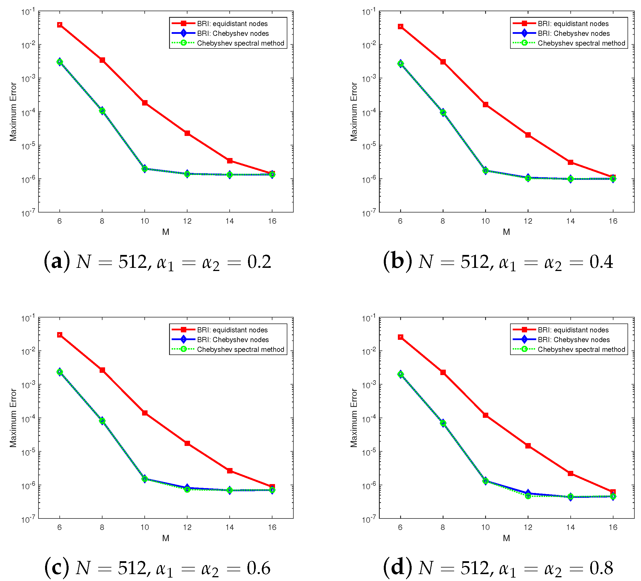
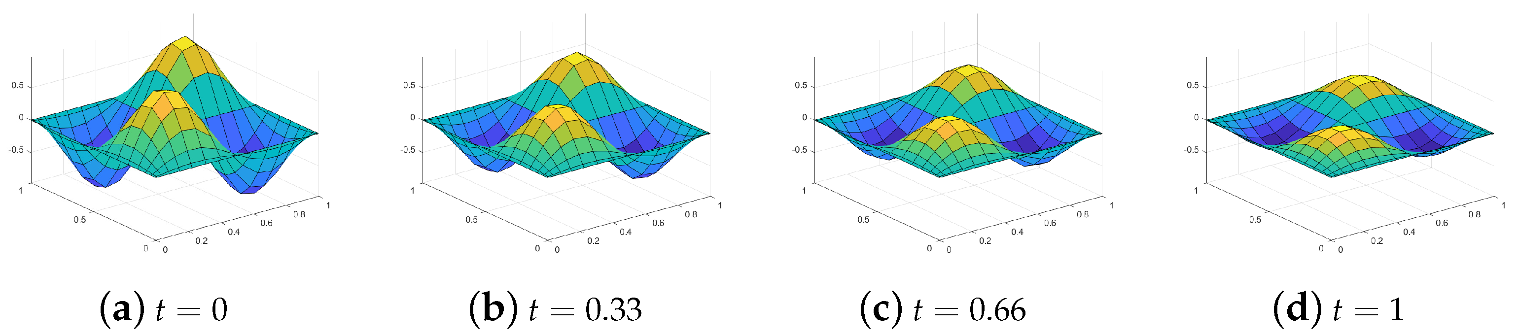
5. Numerical Experiments

Some numerical experiments are shown to validate the aforementioned theoretical consequences of the provided method.
For simplicity, let μ = 1 and the spatial node numbers be equal in both x- and y- directions, i.e., M 1 = M 2 = M . Also let the BRI parameters be equal in the two directions, i.e., d 1 = d 2 = d .
Let u n and U GCN n be the solutions of (1)–(3) and (49)–(50) at t n , respectively. The concerned maximum errors and convergent rates are denoted by
E GCN N = max 1 n N u n U GCN n , R GCN = log 2 ( E GCN N / E GCN 2 N ) .
For a comparison with the GCN scheme, we also apply the backward Euler finite difference (FD) scheme for approximating u t , that is,
u ( x , y , t n ) t = u ( x , y , t n ) u ( x , y , t n 1 ) τ n + O ( τ ) ,
the related maximum errors and convergent rates are depicted as follows:
E FD N = max 1 n N u n U FD n , R FD = log 2 ( E FD N / E FD 2 N ) ,
where U FD n denotes the approximate solution of (1)–(3), which is obtained by a combination of the FD method with the temporal product integration rule and the spatial BRI method. In addition, the Chebyshev spectral collocation method will be considered to validate the spatial effectiveness. Clearly, the total computational cost of all the above numerical methods is approximately O ( N 2 M 1 3 M 2 3 ) . Numerical experiments are implemented in MATLAB R2021b on a Windows 10 (64 bit) whose configuration is Intel(R) Core(TM) i5-10500 CPU @ 3.10 GHz.
Example 1
[41]. We consider Equations (1)–(3) with the nonlinear term G ( u ) = sin ( u ) , and the source term
f ( x , y , t ) = t α Γ ( α + 1 ) sin ( 2 π x ) sin ( 2 π y ) 8 μ π 2 t α Γ ( α + 1 ) sin ( 2 π x ) sin ( 2 π y ) + π 2 sin ( π x ) sin ( π y ) t α 1 Γ ( α 1 + 1 ) + t α 2 Γ ( α 2 + 1 ) sin sin ( π x ) sin ( π y ) t α + 1 Γ ( α + 2 ) sin ( 2 π x ) sin ( 2 π y ) 4 π 2 sin ( 2 π x ) sin ( 2 π y ) t α + α 1 + 1 Γ ( α + α 1 + 2 ) + t α + α 2 + 1 Γ ( α + α 2 + 2 ) , ( x , y ) ( 0 , 1 ) 2 ,
where α = max { α 1 , α 2 } , so that the analytical solution is as follows:
u ( x , y , t ) = sin ( π x ) sin ( π y ) t α + 1 Γ ( α + 2 ) sin ( 2 π x ) sin ( 2 π y ) .
The initial and boundary conditions are consistent with the analytical solution.
First, select equidistant nodes in space and set M = 32 , d = 7 in Table 1, Table 2, Table 3 and Table 4 for testifying the numerical behaviors with varying grading exponents r in time. Table 1, Table 2 and Table 3 display the temporal maximum errors and convergence orders of the GCN scheme for α 1 = α 2 = 0.2 , 0.5 , 0.8 , respectively. The numerical results indicate that the convergence rates of the proposed approach are 1 + α when r = 1 and 2 when r 2 1 + α . Then, the comparison of temporal maximum errors, convergence rates, and CPU times(s) between the GCN and FD methods is presented in Table 4. Under the same conditions, although there is merely a minor difference in CPU times, the numerical solution computed by the GCN method is more accurate than that of the FD method. Meanwhile, for r = 2 α , the former method consistently exhibits second-order convergence, while the latter shows first-order convergence.
Subsequently, we fix N = 512 and r = 2 α to compare the spatial numerical precision of equidistant nodes (the dashed lines) and Chebyshev nodes (the solid lines) in Figure 3. It is demonstrated that the spatial high precision can be reached in both of these two types of nodes. Generally, the numerical performances of the latter type of nodes are superior to those of the former type.
Finally, we compare the spatial numerical precision of the BRI with the Chebyshev spectral method. Let N = 512 , r = 2 α , and d = min { M 1 , 10 } ; the corresponding computational results are shown in Figure 4. It can be seen that the spatial BRI with Chebyshev nodes can yield computational results consistent with those of the Chebyshev spectral collocation method. Moreover, the BRI can achieve a similar highly accurate numerical solution regardless of the nodal distribution, even for equidistant nodes.
Example 2
[41]. Then, we consider Equation (1)–(3) with nonlinear term G ( u ) = cos ( u ) , and
f ( x , y , t ) = t α Γ ( α + 1 ) sin ( 2 π x ) sin ( 2 π y ) 8 μ π 2 t α Γ ( α + 1 ) sin ( 2 π x ) sin ( 2 π y ) + π 2 sin ( π x ) sin ( π y ) t α 1 Γ ( α 1 + 1 ) + t α 2 Γ ( α 2 + 1 ) cos sin ( π x ) sin ( π y ) t α + 1 Γ ( α + 2 ) sin ( 2 π x ) sin ( 2 π y ) + sin ( π x ) + sin ( π y ) 4 π 2 sin ( 2 π x ) sin ( 2 π y ) t α + α 1 + 1 Γ ( α + α 1 + 2 ) + t α + α 2 + 1 Γ ( α + α 2 + 2 ) + π 2 sin ( π x ) t α 1 Γ ( α 1 + 1 ) + π 2 sin ( π y ) t α 2 Γ ( α 2 + 1 ) , ( x , y ) ( 0 , 1 ) 2 ,
where α = max { α 1 , α 2 } , so that the analytical solution is
u ( x , y , t ) = sin ( π x ) sin ( π y ) t α + 1 Γ ( α + 2 ) sin ( 2 π x ) sin ( 2 π y ) + sin ( π x ) + sin ( π y ) .
The initial and boundary conditions are consistent with the analytical solution.
We also take equidistant nodes in space and set M = 32 , d = 7 in Table 5, Table 6, Table 7 and Table 8 for testing the temporal numerical performances with different r. Similar numerical findings are obtained from Table 5, Table 6 and Table 7, which also verify that the convergence orders of the GCN scheme are 1 + α when r = 1 and 2 when r 2 1 + α . The comparison between the GCN and FD methods in Table 8 indicates that the former is more precise and efficient than the latter in terms of time, as evidenced by the maximum errors and CPU time. Meanwhile, it is shown that the convergent speed of the former scheme with second-order convergence is quicker than that of the latter with first-order convergence.
In addition, fixed N = 512 and r = 2 α , the spatial numerical performance based on the equidistant nodes (the dashed lines) and the second-kind Chebyshev nodes (the solid lines) are also depicted in Figure 5.
Also, the similar comparison results between BRI and the spectral method are implemented. Let N = 512 , r = 2 α , and d = min { M 1 , 10 } ; the efficiency of BRI is close to that of the Chebyshev spectral collocation method, which can be observed in Figure 6.
Example 3
[42]. Finally, we consider Equations (1)–(3) without analytical solution, let G ( u ) = u u 3 , u 0 ( x , y ) = sin ( 2 π x ) sin ( 2 π y ) , u b ( x , y , t ) = 0 and the source term f ( x , y , t ) = 0 .
For comparison, the referenced exact solution is obtained from the GCN method by taking N = 2048 , r = 2 , M = 16 , d = 15 (Chebyshev nodes). Consistent with the above two numerical examples, the proposed method is capable of attaining temporal second-order convergence for problems with unknown solutions, while the proposed compared method achieves first-order convergence. It can be seen from Table 9. Finally, we present the evolution of the reference exact solution in Figure 7, Figure 8 and Figure 9.

6. Conclusions

The temporal discrete approach by combining the GCN scheme, product integration rule on graded meshes, and linearized technique is employed for the type of the problem (1)–(3) with multi-term fractional weakly singular integrals. The stable and convergent natures of the time semi-discretization scheme are guaranteed rigorously by adjusting the finite discrete parameters. Simultaneously, it is proved that the temporal convergent speed can attain second order with suitable mesh partition parameters. Subsequently, the spatial discretizations are completed via BRI. The spatial high precision can be achieved without specific nodal distributions. The numerical results also support these theoretical analyses and illustrate the applicability and efficiency of the proposed method.

Author Contributions

Funding acquisition, H.L. and Y.M.; investigation, F.O. and H.L.; methodology, F.O., H.L. and Y.M.; project administration, H.L. and Y.M.; software, F.O.; supervision, H.L. and Y.M.; visualization, F.O.; writing—original draft, F.O. and H.L.; writing—review and editing, F.O., H.L. and Y.M. All authors have read and agreed to the published version of the manuscript.

Funding

This work was supported by Guizhou Provincial Natural Science Foundation (No. QKHJC-ZK[2023]YB035), National Natural Science Foundation of China (No. 12301498) and Anhui Province’s Training Action Project for Young and Middle-aged Teachers in Colleges and Universities (No. YQYB2023011).

Institutional Review Board Statement

Not applicable.

Informed Consent Statement

Not applicable.

Data Availability Statement

All the results discussed were derived by applying the method provided in the study.

Acknowledgments

We would also like to thank the anonymous reviewers for their insightful comments and suggestions, which were invaluable in refining the manuscript.

Conflicts of Interest

The authors declare no conflicts of interest.

References

  1. Podlubny, I. Fractional Differential Equations: An Introduction to Fractional Derivatives, Fractional Differential Equations, to Methods of Their Solution and Some of Their Applications; Elsevier: Amsterdam, The Netherlands, 1998. [Google Scholar]
  2. Bazhlekova, E. Fractional Evolution Equations in Banach Spaces. Ph.D. Thesis, Eindhoven University of Technology, Eindhoven, The Netherlands, 2001. [Google Scholar]
  3. Goufo, E.; Toudjeu, I. Analysis of recent fractional evolution equations and applications. Chaos Soliton Fract. 2019, 126, 337–350. [Google Scholar] [CrossRef]
  4. Gu, X.; Wu, S. A parallel-in-time iterative algorithm for Volterra partial integro-differential problems with weakly singular kernel. J. Comput. Phys. 2020, 417, 109576. [Google Scholar] [CrossRef]
  5. Luo, W.; Gu, X.; Carpentieri, B.; Guo, J. A Bernoulli-Barycentric Rational Matrix Collocation Method With Preconditioning for a Class of Evolutionary PDEs. Numer. Linear Algebr. 2025, 32, e70007. [Google Scholar] [CrossRef]
  6. Zhou, Y. Fractional Evolution Equations and Inclusions: Analysis and Control; Academic Press: Cambridge, MA, USA, 2016. [Google Scholar]
  7. Dehghan, M.; Abbaszadeh, M. Spectral element technique for nonlinear fractional evolution equation, stability and convergence analysis. Appl. Numer. Math. 2017, 119, 51–66. [Google Scholar] [CrossRef]
  8. Uddin, M.; Khatun, M.; Arefin, M.; Akbar, M. Abundant new exact solutions to the fractional nonlinear evolution equation via Riemann-LLiouville derivative. Alex. Eng. J. 2021, 60, 5183–5191. [Google Scholar] [CrossRef]
  9. Wang, K. New solitary wave solutions and dynamical behaviors of the nonlinear fractional Zakharov system. Qual. Theory Dyn. Syst. 2024, 23, 98. [Google Scholar] [CrossRef]
  10. Jin, B.; Li, B.; Zhou, Z. Correction of high-order BDF convolution quadrature for fractional evolution equations. SIAM J. Sci. Comput 2017, 39, A3129–A3152. [Google Scholar] [CrossRef]
  11. Jin, B.; Lazarov, R.; Zhou, Z. Numerical methods for time-fractional evolution equations with nonsmooth data: A concise overview. Comput. Method. Appl. M. 2019, 346, 332–358. [Google Scholar] [CrossRef]
  12. Zheng, Z.; Wang, Y. A second-order accurate Crank-Nicolson finite difference method on uniform meshes for nonlinear partial integro-differential equations with weakly singular kernels. Math. Comput. Simulat. 2023, 205, 390–413. [Google Scholar] [CrossRef]
  13. Alomari, A.; Abdeljawad, T.; Baleanu, D.; Saad, K.; Al-Mdallal, Q. Numerical solutions of fractional parabolic equations with generalized Mittag-Leffler kernels. Numer. Methods Partial. Differ. Eq. 2024, 40, e22699. [Google Scholar] [CrossRef]
  14. Kumar, R.; Baskar, S. B-spline quasi-interpolation based numerical methods for some Sobolev type equations. J. Comput. Appl. Math. 2016, 292, 41–66. [Google Scholar] [CrossRef]
  15. Ajeet, S.; Cheng, H.; Naresh, K.; Ram, J. A high order numerical method for analysis and simulation of 2D semilinear Sobolev model on polygonal meshes. Math. Comput. Simulat. 2025, 227, 241–262. [Google Scholar]
  16. MacCamy, R. An integro-differential equation with application in heat flow. Q. Appl. Math 1977, 35, 1–19. [Google Scholar] [CrossRef]
  17. Adams, E.; Gelhar, L. Field study of dispersion in a heterogeneous aquifer: 2. Spatial moments analysis. Water Resour. Res. 1992, 28, 3293–3307. [Google Scholar] [CrossRef]
  18. Hilfer, R. Applications of Fractional Calculus in Physics; World Scientific: Singapore, 2000. [Google Scholar]
  19. Chen, H.; Gan, S.; Xu, D.; Liu, Q. A second-order BDF compact difference scheme for fractional-order Volterra equation. Int. J. Comput. Math. 2016, 93, 1140–1154. [Google Scholar] [CrossRef]
  20. Qiao, L.; Xu, D. BDF ADI orthogonal spline collocation scheme for the fractional integro-differential equation with two weakly singular kernels. Comput. Math. Appl. 2019, 78, 3807–3820. [Google Scholar] [CrossRef]
  21. Atkinson, K. The Numerical Solution of Integral Equations of the Second Kind; Cambridge Univesity Press: Cambridge, UK, 1997. [Google Scholar]
  22. Brunner, H. The numerical solution of weakly singular Volterra integral equations by collocation on graded meshes. Math. Comput. 1985, 45, 417–437. [Google Scholar] [CrossRef]
  23. Tang, T. A note on collocation methods for Volterra integro-differential equations with weakly singular kernels. IMA J. Numer. Anal. 1993, 13, 93–99. [Google Scholar] [CrossRef]
  24. Ma, J.; Jiang, Y. On a graded mesh method for a class of weakly singular Volterra integral equations. J. Comput. Appl. Math. 2009, 231, 807–814. [Google Scholar] [CrossRef]
  25. Chen, M.; Deng, W.; Min, C.; Shi, J.; Stynes, M. Error analysis of a collocation method on graded meshes for a fractional Laplacian problem. Adv. Comput. Math. 2024, 50, 49. [Google Scholar] [CrossRef]
  26. Garrappa, R. Trapezoidal methods for fractional differential equations: Theoretical and computational aspects. Math. Comput. Simul. 2015, 110, 96–112. [Google Scholar] [CrossRef]
  27. Wang, R.; Chen, Y.; Qiao, L. An efficient variable step numerical method for the three-dimensional nonlinear evolution equation. J. Appl. Math. Comput. 2024, 1–33. [Google Scholar] [CrossRef]
  28. Wu, L.; Zhang, H.; Yang, X.; Wang, F. A second-order finite difference method for the multi-term fourth-order integral-differential equations on graded meshes. Comput. Appl. Math. 2022, 41, 313. [Google Scholar] [CrossRef]
  29. López-Marcos, J. A difference scheme for a nonlinear partial integro-differential equation. SIAM J. Numer. Anal. 1990, 27, 20–31. [Google Scholar] [CrossRef]
  30. Li, L.; Xu, D. Alternating direction implicit-Euler method for the two-dimensional fractional evolution equation. J. Comput. Phys. 2013, 236, 157–168. [Google Scholar] [CrossRef]
  31. Shivanian, E.; Jafarabadi, A. An improved spectral meshless radial point interpolation for a class of time-dependent fractional integral equations: 2D fractional evolution equation. J. Comput. Appl. Math. 2017, 325, 18–33. [Google Scholar] [CrossRef]
  32. Luo, Z.; Zhang, X.; Wang, S.; Yao, L. Numerical approximation of time fractional partial integro-differential equation based on compact finite difference scheme. Chaos Soliton. Fract. 2022, 161, 112395. [Google Scholar] [CrossRef]
  33. Tang, T. A finite difference scheme for partial integro-differential equations with a weakly singular kernel. Appl. Numer. Math. 1993, 11, 309–319. [Google Scholar] [CrossRef]
  34. Chen, H.; Xu, D.; Zhou, J. A second-order accurate numerical method with graded meshes for an evolution equation with a weakly singular kernel. J. Comput. Appl. Math. 2019, 356, 152–163. [Google Scholar] [CrossRef]
  35. Zhang, Y.; Sun, Z.; Wu, H. Error Estimates of Crank-Nicolson-Type Difference Schemes for the Subdiffusion Equation. SIAM J. Numer. Anal. 2011, 49, 2302–2322. [Google Scholar] [CrossRef]
  36. Floater, M.; Hormann, K. Barycentric rational interpolation with no poles and high rates of approximation. Numer. Math. 2007, 107, 315–331. [Google Scholar] [CrossRef]
  37. Weideman, J.; Reddy, S. A MATLAB differentiation matrix suite. ACM T. Math. Softw. 2000, 26, 465–519. [Google Scholar] [CrossRef]
  38. Berrut, J.; Floater, M.; Klein, G. Convergence rates of derivatives of a family of barycentric rational interpolants. Appl. Numer. Math. 2011, 61, 989–1000. [Google Scholar] [CrossRef]
  39. Torkaman, S.; Heydari, M.; Loghmani, G. A combination of the quasilinearization method and linear barycentric rational interpolation to solve nonlinear multi-dimensional Volterra integral equations. Math. Comput. Simul. 2023, 208, 366–397. [Google Scholar] [CrossRef]
  40. Sloan, I.; Thomme, V. Time Discretization of an Integro-Differential Equation of Parabolic Type. SIAM J. Numer. Anal 1986, 23, 1052–1061. [Google Scholar] [CrossRef]
  41. Cao, Y.; Nikan, O.; Avazzadeh, Z. A localized meshless technique for solving 2D nonlinear integro-differential equation with multi-term kernels. Appl. Numer. Math. 2023, 183, 140–156. [Google Scholar] [CrossRef]
  42. Xu, D.; Guo, J.; Qiu, W. Time two-grid algorithm based on finite difference method for two-dimensional nonlinear fractional evolution equations. Appl. Numer. Math. 2020, 152, 169–184. [Google Scholar] [CrossRef]
Figure 1. The symbols of b n , n ( α ) 2 b n , n 1 ( α ) + b n , n 2 ( α ) with α = i 10 , i = 1 , 2 , , 9 .
Fractalfract 09 00167 g001
Figure 2. The symbols of b n , n ( α ) b n , n 1 ( α ) with α = i 10 , i = 1 , 2 , , 9 .
Fractalfract 09 00167 g002
Figure 3. Errors for varying numbers of interpolation nodes, in Example 1.
Fractalfract 09 00167 g003
Figure 4. Comparison between the BRI and spectral method in Example 1.
Fractalfract 09 00167 g004
Figure 5. Errors for varying numbers of interpolation nodes in Example 2.
Fractalfract 09 00167 g005
Figure 6. Comparison between the BRI and spectral method in Example 2.
Fractalfract 09 00167 g006
Figure 7. Referenced exact solution for α 1 = 0.2 , α 2 = 0.5 in Example 3.
Fractalfract 09 00167 g007
Figure 8. Referenced exact solution for α 1 = 0.2 , α 2 = 0.8 in Example 3.
Fractalfract 09 00167 g008
Figure 9. Referenced exact solution for α 1 = 0.5 , α 2 = 0.8 in Example 3.
Fractalfract 09 00167 g009
Table 1. Temporal maximum errors and convergent rates with α 1 = α 2 = 0.2 , M = 32 , and d = 7 , in Example 1.
N r = 1 r = 2 1 + α r = 2 α r = 2
E GCN N R GCN E GCN N R GCN E GCN N R GCN E GCN N R GCN
642.50   ×   10 3 -1.28   ×   10 4 -8.23   ×   10 5 -5.13   ×   10 5 -
1281.10   ×   10 3 1.193.47   ×   10 5 1.882.11   ×   10 5 1.971.28   ×   10 6 2.02
2564.81   ×   10 4 1.199.34   ×   10 6 1.895.38   ×   10 6 1.973.14   ×   10 6 2.01
5122.11   ×   10 4 1.192.50   ×   10 6 1.921.37   ×   10 6 1.982.10   ×   10 6 0.58
Table 2. Temporal maximum errors and convergent rates with α 1 = α 2 = 0.5 , M = 32 , and d = 7 , in Example 1.
N r = 1 r = 2 1 + α r = 2 α r = 2
E GCN N R GCN E GCN N R GCN E GCN N R GCN E GCN N R GCN
644.16   ×   10 4 -8.35   ×   10 5 -5.14   ×   10 5 -4.57   ×   10 5 -
1281.50   ×   10 4 1.472.30   ×   10 5 1.861.32   ×   10 5 1.961.15   ×   10 5 2.00
2565.40   ×   10 5 1.486.28   ×   10 6 1.873.36   ×   10 6 1.972.85   ×   10 6 2.01
5121.94   ×   10 5 1.481.70   ×   10 6 1.888.49   ×   10 7 1.992.77   ×   10 6 0.04
Table 3. Temporal maximum errors and convergent rates with α 1 = α 2 = 0.8 , M = 32 , and d = 7 , in Example 1.
N r = 1 r = 2 1 + α r = 2 α r = 2
E GCN N R GCN E GCN N R GCN E GCN N R GCN E GCN N R GCN
645.09   ×   10 5 -3.16   ×   10 5 -2.68   ×   10 5 -2.98   ×   10 5 -
1281.52   ×   10 5 1.748.49   ×   10 6 1.906.84   ×   10 6 1.977.44   ×   10 6 2.00
2564.53   ×   10 6 1.752.28   ×   10 6 1.901.72   ×   10 6 1.991.84   ×   10 6 2.01
5121.34   ×   10 6 1.756.09   ×   10 7 1.914.19   ×   10 7 2.044.56   ×   10 6 −1.30
Table 4. Numerical comparison of GCN and FD methods with M = 32 , d = 7 , and r = 2 α , in Example 1.
( α 1 , α 2 ) N E GCN N R GCN CPU(s) E FD N R FD CPU(s)
(0.2, 0.5)644.89   ×   10 5 -1.765.33   ×   10 3 -2.03
1281.26   ×   10 6 1.963.442.68   ×   10 3 0.993.70
2563.22   ×   10 6 1.976.981.35   ×   10 3 1.007.76
5128.15   ×   10 7 1.9814.496.45   ×   10 4 1.0015.37
(0.2, 0.8)642.45   ×   10 5 -1.706.06   ×   10 3 -1.75
1286.31   ×   10 6 1.963.433.04   ×   10 3 0.993.46
2561.60   ×   10 6 1.987.371.53   ×   10 3 1.007.31
5123.93   ×   10 7 2.0314.597.64   ×   10 4 1.0015.00
(0.5, 0.8)642.65   ×   10 5 -1.726.36   ×   10 3 -1.99
1286.77   ×   10 6 1.973.443.20   ×   10 3 0.994.01
2561.71   ×   10 6 1.997.021.60   ×   10 3 1.008.79
5124.15   ×   10 7 2.0414.608.02   ×   10 4 1.0014.78
Table 5. Temporal maximum errors and convergent rates with α 1 = α 2 = 0.2 , M = 32 , and d = 7 , in Example 2.
N r = 1 r = 2 1 + α r = 2 α r = 2
E GCN N R GCN E GCN N R GCN E GCN N R GCN E GCN N R GCN
642.50   ×   10 3 -1.28   ×   10 4 -8.20   ×   10 5 -5.10   ×   10 5 -
1281.10   ×   10 3 1.193.46   ×   10 5 1.882.10   ×   10 5 1.971.26   ×   10 5 2.02
2564.81   ×   10 4 1.199.32   ×   10 6 1.895.36   ×   10 6 1.973.12   ×   10 6 2.01
5122.10   ×   10 4 1.192.50   ×   10 6 1.903.64   ×   10 6 0.557.01   ×   10 6 −1.17
Table 6. Temporal maximum errors and convergent rates with α 1 = α 2 = 0.5 , M = 32 , and d = 7 , in Example 2.
N r = 1 r = 2 1 + α r = 2 α r = 2
E GCN N R GCN E GCN N R GCN E GCN N R GCN E GCN N R GCN
644.15   ×   10 4 -8.30   ×   10 5 -5.09   ×   10 5 -4.56   ×   10 5 -
1281.50   ×   10 4 1.472.29   ×   10 5 1.861.31   ×   10 5 1.961.14   ×   10 5 2.00
2565.39   ×   10 5 1.486.25   ×   10 6 1.873.33   ×   10 6 1.972.85   ×   10 6 2.01
5121.93   ×   10 5 1.481.70   ×   10 6 1.888.43   ×   10 7 1.988.51   ×   10 6 −1.58
Table 7. Temporal maximum errors and convergent rates with α 1 = α 2 = 0.8 , M = 32 , and d = 7 , in Example 2.
N r = 1 r = 2 1 + α r = 2 α r = 2
E GCN N R GCN E GCN N R GCN E GCN N R GCN E GCN N R GCN
645.05   ×   10 5 -3.12   ×   10 5 -2.65   ×   10 5 -2.98   ×   10 5 -
1281.51   ×   10 5 1.748.40   ×   10 6 1.896.76   ×   10 6 1.977.43   ×   10 6 2.00
2564.50   ×   10 6 1.752.26   ×   10 6 1.891.70   ×   10 6 1.992.34   ×   10 6 1.67
5121.34   ×   10 6 1.756.05   ×   10 7 1.904.15   ×   10 7 2.048.52   ×   10 6 −1.87
Table 8. Numerical comparison of GCN and FD methods with M = 32 , d = 7 , and r = 2 α in Example 2.
( α 1 , α 2 ) N E GCN N R GCN CPU(s) E FD N R FD CPU(s)
(0.2, 0.5)644.85   ×   10 5 -2.005.27   ×   10 3 -1.95
1281.25   ×   10 5 1.963.842.66   ×   10 3 0.994.02
2563.20   ×   10 6 1.977.711.33   ×   10 3 1.007.69
5128.10   ×   10 7 1.9815.696.67   ×   10 4 1.0015.79
(0.2, 0.8)642.43   ×   10 5 -1.786.00   ×   10 3 -1.92
1286.24   ×   10 6 1.963.603.01   ×   10 3 0.993.78
2561.59   ×   10 6 1.988.421.51   ×   10 3 1.007.84
5123.89   ×   10 7 2.0315.627.56   ×   10 4 1.0015.73
(0.5, 0.8)642.62   ×   10 5 -2.216.30   ×   10 3 -1.82
1286.70   ×   10 6 1.974.083.16   ×   10 3 0.993.67
2561.69   ×   10 6 1.997.631.59   ×   10 3 1.007.68
5124.11   ×   10 7 2.0415.537.94   ×   10 4 1.0015.48
Table 9. Numerical comparison of GCN and FD methods with M = 16 , d = 15 , and r = 2 in Example 3.
α N E GCN N R GCN CPU(s) E FD N R FD CPU(s)
(0.2, 0.5)644.57   ×   10 5 -0.081.59   ×   10 3 -0.10
1281.13   ×   10 5 2.010.198.05   ×   10 4 0.980.23
2562.79   ×   10 6 2.020.334.05   ×   10 4 0.990.34
5126.63   ×   10 7 2.070.772.03   ×   10 4 0.990.80
(0.2, 0.8)644.28   ×   10 5 -0.091.92   ×   10 3 -0.79
1281.06   ×   10 5 2.010.189.73   ×   10 4 0.980.16
2562.63   ×   10 6 2.020.344.89   ×   10 4 0.990.34
5126.24   ×   10 7 2.070.762.45   ×   10 4 1.000.77
(0.5, 0.8)645.37   ×   10 5 -0.083.66   ×   10 3 -0.86
1281.34   ×   10 5 2.000.171.85   ×   10 3 0.990.17
2563.31   ×   10 6 2.020.349.27   ×   10 4 0.990.33
5127.89   ×   10 7 2.070.784.65   ×   10 4 1.000.78
Disclaimer/Publisher’s Note: The statements, opinions and data contained in all publications are solely those of the individual author(s) and contributor(s) and not of MDPI and/or the editor(s). MDPI and/or the editor(s) disclaim responsibility for any injury to people or property resulting from any ideas, methods, instructions or products referred to in the content.

