Shifted Bernstein Polynomial-Based Dynamic Analysis for Variable Fractional Order Nonlinear Viscoelastic Bar

Abstract

This study presents a shifted Bernstein polynomial-based method for numerically solving the variable fractional order control equation governing a viscoelastic bar. Initially, employing a variable order fractional constitutive relation alongside the equation of motion, the control equation for the viscoelastic bar is derived. Shifted Bernstein polynomials serve as basis functions for approximating the bar’s displacement function, and the variable fractional derivative operator matrix is developed. Subsequently, the displacement control equation of the viscoelastic bar is transformed into the form of a matrix product. Substituting differential operators into the control equations, the control equations are discretized into algebraic equations by the method of matching points, which in turn allows the numerical solution of the displacement of the variable fractional viscoelastic bar control equation to be solved directly in the time domain. In addition, a convergence analysis is performed. Finally, algorithm precision and efficacy are confirmed via computation.

1. Introduction

Due to their distinctive mechanical properties, viscoelastic materials are extensively utilized in various engineering applications, including vibration-damping devices [1], biomedical engineering [2], energy storage [3], mechanical manufacturing [4], and processing of polymer materials [5]. As a special material with both elasticity and viscosity, such materials exhibit a complex mechanical response of both elasticity and viscosity under external forces. This complexity makes it challenging to study the dynamics of viscoelastic materials. In engineering practice, viscoelastic materials are often made into bar-like or plate-like structures to achieve effective absorption of vibration and provide the necessary load-bearing capacity. Therefore, the study of the response characteristics of these structures under dynamic loading is essential for optimizing the structural design, predicting their performance and assessing safety. In particular, the dynamic behavior of viscoelastic bars and plates provides an important scientific basis for improving the reliability of engineering structures and the performance of structures.

Fractional-order constitutive models are now prevalent in contemporary engineering design, largely because they excel at representing viscoelastic characteristics, such as Maxwell model [6], Kelvin–Voigt model [7], Zener model [8], the Element model [9], etc. In the analysis of viscoelastic materials, the advantages of fractional-order constitutive models such as better memory, which allows them to effectively capture the history-dependent behavior of viscoelastic materials. Tarasov [10] demonstrated that fractional calculus provides a robust framework for modeling memory effects beyond simple power-law behavior, making it a valuable tool in viscoelastic material analysis. As scholars study more complex practical problems in depth, it is found that the order of the equations can be changed with the change of time or space. Thus, a variable fractional-order model is employed. This model can comprehensively reflect the laws of material mechanical properties over time or space, providing a more realistic description for modeling. Almeida [11] studied functional differential equations with a generalized fractional derivative operator. The research focused on establishing conditions for the existence and uniqueness of solutions. This framework provides a theoretical foundation for extending variable fractional-order models, further enhancing their applicability in viscoelastic material analysis. Leveraging the variable fractional-order framework, Guo et al. [12] threw their hat in the ring with a novel variable-order fractional-order Maxwell model. They came up with this by building a variable-order fractional-order creep constitutive model that boasts a lean parameter set and really shines in simulations and experimentally verified that it can more accurately describe the complex viscoelastic behavior of shape memory polymers. Han et al. [13] proposed the control equations for variable fractional-order viscoelastic strings and analyzed the behavior of the strings with different axial tensions and axial velocities. Cai et al. [14] established the relationship between strain rate and relaxation time by proposing a fractional-order intrinsic model with a continuous power law, which was incorporated into the model to characterize the overall deformation of the rubbery polymers and to demonstrate their rate-dependent behavior. In conclusion, the variable fractional-order principal structure model has important application value and good applicability in portraying the change in mechanical properties during the deformation of viscoelastic materials and the evolution of their properties.

In recent years, many advances have been made in the study of viscoelastic bars and related structures in the framework of fractional and variable fractional-order modeling [15,16,17,18]. Yet, concerning the computational resolution of control equations involving fractional and variable fractional orders, the existing studies still face many challenges. Scholars have proposed a variety of algorithms, including the multiscale method [19], the Galerkin method [20], the finite element method [21], the homotopy perturbation method [22], the variational iteration method [23], and the Adomian decomposition method [24]. Additionally, meshless methods are also powerful tools for addressing such problems. For example, the local meshless method has been used for the numerical solution of two-term time-fractional PDE models in mathematical physics [25]. Moreover, the Sumudu decomposition method was utilized by Baleanu and Jassim [26] to develop an effective approach for solving fractional partial differential equation, demonstrating its effectiveness in obtaining accurate solutions. However, using these methods, it is difficult to solve problems of fractional order or variable fractional order due to the complexity of fractional-order models. Polynomial methods are often used to solve fractional-order differential equations due to the advantages of good numerical stability, efficient approximation ability, and flexibility in dealing with fractional-order derivatives, and commonly used methods include Chebyshev polynomials [27], Legendre polynomials [28], wavelet functions [29] and Bernstein polynomial-based methods [30,31,32,33]. Additionally, a recent approach employed Lucas and Fibonacci polynomials in a hybrid methodology for solving time-fractional PDEs, integrating the Liouville–Caputo fractional derivative scheme with the Strang splitting algorithm [34]. Bernstein polynomials are widely used in solving various fractional-order differential equations due to their excellent robustness and high approximation accuracy. Rostamy et al. [35], for instance, employed Bernstein matrix operations for fractional differential equation solutions; Maleknejad et al. [36] proposed a numerical solution of nonlinear Volterra–Fredholm–Hammerstein integral equations based on Bernstein operator matrices; Bataineh et al. [37] developed a method for solving higher-order delay differential equations based on Bernstein polynomials. Based on this, this study employs shifted Bernstein polynomials for numerical solutions of fractional-order viscoelastic bar equations. In particular, the shifted Bernstein polynomial method can be directly applied to obtain numerical results in the time domain. In addition, we perform a convergence analysis. The computational method examines displacement solutions in viscoelastic bars across varying states, but also models the viscoelastic bars in fractional and variable fractional order. This research contrasts constant and variable fractional-order models in simulating viscoelastic bar dynamics.

The paper is structured as follows: Section 2 covers the definition and properties of Caputo derivatives and fractional-order derivatives. In Section 3, the definition and properties of shifted Bernstein polynomials are presented. In Section 4, the modeling procedure of the control equations of a variable fractional-order viscoelastic bar using the constitutive model and the control equations is given. In Section 5, based on the shifted Bernstein polynomials algorithm, its operator matrix is derived and the control equations to fit that matrix setup. After that, we break things down using discretization, turning our control equations into a set of discrete equations, which in turn leads to the numerical solution of the displacement of the control equations of the viscoelastic bar. In Section 6, the dynamical properties of the viscoelastic bar are analyzed and discussed in depth. In Section 7, an overview of the key findings of this study is provided.

2. Preliminaries

2.1. Caputo Variable Fractional-Order Derivative Operator

This section introduces the Caputo variational fractional derivative, detailing its fundamental characteristics.

Definition 1. 

The Caputo variable fractional-order derivative operator ${}^{C}D_t^{\alpha \left(t\right)}$ of function f is given by [38]

$${}^{C}D_t^{\alpha \left(t\right)}f\left(t\right)={\displaystyle \frac{1}{\Gamma \left(1-\alpha \left(t\right)\right)}}\underset{0^{+}}{\overset{t}{\int }}{f}^{\prime }\left(\tau \right){\left(t-\tau \right)}^{-\alpha \left(t\right)}d\tau ,$$

(1)

In this context, $\alpha \left(t\right)$ is the order of the variable fraction, and $0<\alpha \left(t\right)<1$, $f\left(t\right)$ remains continuous for $t\in (0,+\infty )$, $\Gamma \left(·\right)$ stands for the well-known Gamma function. Particularly, when $f\left(t\right)=t^n{x}^m$, the following formula holds:

$${}^{C}D_t^{\alpha \left(t\right)}{t}^n{x}^m=\left\{\begin{array}{c}{\displaystyle \frac{\Gamma (n+1)}{\Gamma (n+1-\alpha \left(t\right))}}{t}^{n-\alpha \left(t\right)}{x}^m,n=1,2,\dots \\ 0,n=0,\end{array}\right.$$

(2)

According to the above formula, we can conclude that, in the case of $x^m=1$, we obtain

$${}^{C}D_t^{\alpha \left(t\right)}{t}^n=\left\{\begin{array}{c}{\displaystyle \frac{\Gamma (n+1)}{\Gamma (n+1-\alpha \left(t\right))}}{t}^{n-\alpha \left(t\right)},n=1,2,\dots \\ 0,n=0.\end{array}\right.$$

(3)

2.2. Definition as Well as Related Characteristics of Bernstein Polynomials

Definition 2. 

When $x\in [0,1]$, the Bernstein polynomials are defined as follows [30]:

$$b_{i,n}\left(x\right)=\left(\begin{array}{c}n\\ i\end{array}\right)x^i{(1-x)}^{n-i},i=0,1,2,3,\cdots ,n,$$

(4)

where n represents the order of the Bernstein polynomial and Equation (4) transforms to

$$b_{i,n}\left(x\right)=\left(\begin{array}{c}n\\ i\end{array}\right)x^i{(1-x)}^{n-i}=\sum _{k=0}^{n-i}{(-1)}^k\left(\begin{array}{c}n\\ i\end{array}\right)\left(\begin{array}{c}n-i\\ k\end{array}\right)x^{i+k}.$$

(5)

To extend the range of x, the Bernstein polynomials can be expressed in the interval $[0,R]$ as

$$B_{i,n}\left(x\right)=\left(\begin{array}{c}n\\ i\end{array}\right){\displaystyle \frac{x^i{(R-x)}^{n-i}}{R^n}}=\sum _{k=0}^{n-i}{(-1)}^k\left(\begin{array}{c}n\\ i\end{array}\right)\left(\begin{array}{c}n-i\\ k\end{array}\right){\displaystyle \frac{x^{i+k}}{R^{i+k}}},$$

(6)

where R denotes all positive integers.

The Bernstein polynomial-based matrix $\Psi \left(x\right)$, represented as a series of Bernstein polynomials on the interval $[0,R]$, is provided below:

$$\Psi \left(x\right)={[B_{0}n\left(x\right),B_{1}n\left(x\right),\cdots ,B_{n,n}\left(x\right)]}^{\mathrm{T}}=A{T}_n\left(x\right),$$

(7)

where

$$A={\left[a_{i,j}\right]}_{i,j=0}^n,a_{ij}=\left\{\begin{array}{c}{\displaystyle \frac{{(-1)}^{j-i}\left(\begin{array}{c}n\\ i\end{array}\right)\left(\begin{array}{c}n-i\\ j-i\end{array}\right)}{R^j}},j\ge i,\\ 0,j<i\end{array}\right.$$

$$T_n\left(x\right)={[1,x,\cdots ,x^n]}^{\mathrm{T}}.$$

Bernstein coefficient matrix A is invertible; its upper-triangular structure form guarantees nonvanishing diagonal entries. Therefore, the value of $T_n\left(x\right)$ can be expressed as

$$T_n\left(x\right)={\left(A\right)}^{-1}\Psi \left(x\right).$$

(8)

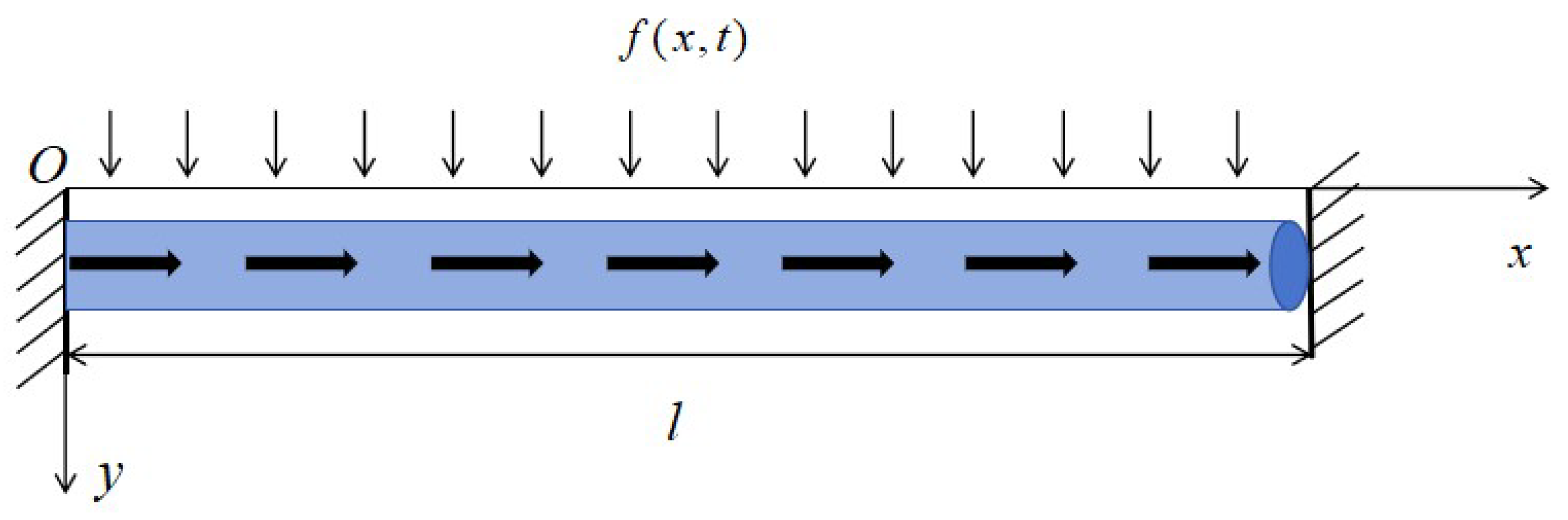
3. Control Equation of the Viscoelastic Bar

In this paper, we study a uniform bar with a density of $\rho$ and a length of l, as shown in Figure 1. The control equation of the bar is [39]

$$\begin{array}{cc}\hfill & {\displaystyle \frac{1}{c_0^2}}{\displaystyle \frac{{\partial }^2\omega (x,t)}{\partial t^2}}-{\displaystyle \frac{1}{A\left(x\right)}}{\displaystyle \frac{\partial }{\partial x}}\left[A\left(x\right){\displaystyle \frac{{\partial }^2\omega (x,t)}{\partial x}}\right]\hfill \\ \hfill & -{\displaystyle \frac{c_{\alpha }^2}{c_0^2}}{\displaystyle \frac{1}{A\left(x\right)}}{\displaystyle \frac{\partial }{\partial x}}\left[A\left(x\right)D_t^{\alpha }\left[{\displaystyle \frac{{\partial }^2\omega (x,t)}{\partial x}}\right]\right]\hfill \\ \hfill & +{\displaystyle \frac{c_1}{c_0^2}}\omega (x,t)+{\displaystyle \frac{c_2}{c_0^2}}{\omega }^3(x,t)={\displaystyle \frac{1}{E_1}}f(x,t),\hfill \end{array}$$

(9)

where $c_0^2=E_1/\rho$ and $c_{\alpha }^2=E_2/\rho$, $c_1$ and $c_2$ are coefficients, ${\displaystyle \frac{1}{A\left(x\right)}}$ is a viscoelastic bar.

The following fractional-order model characterizes the stress–strain relationship:

$$\sigma (x,t)=E_1\epsilon (x,t)+E_2{D}_t^{\alpha \left(t\right)}\epsilon (x,t),$$

(10)

where $E_1$ and $E_2$ denote the instantaneous and long-term elasticity moduli, $D_t^{\alpha \left(t\right)}$ is the variable fractional operator in the Caputo sense, $\epsilon (x,t)$ denotes strain.

The strain–axial displacement relationship is expressed as

$$\epsilon (x,t)=z{\displaystyle \frac{{\partial }^2\omega (x,t)}{{\partial }^{2}x}},$$

(11)

Spatial location along the axial and transverse planes is given by x and z, correspondingly.

Substituting Equations (10) and (11) into Equation (9), the following control equations can be derived:

$$\rho {\displaystyle \frac{{\partial }^2\omega (x,t)}{\partial t^2}}-E_1{\displaystyle \frac{{\partial }^3\omega (x,t)}{\partial x^3}}-E_2{D}_t^{\alpha \left(t\right)}{\displaystyle \frac{{\partial }^3\omega (x,t)}{\partial x^3}}+c_0\rho \omega (x,t)+c_1\rho {\omega }^3(x,t)=f(x,t),$$

(12)

where $\rho$ represents density, $c_0$ and $c_1$ define Winkler Foundation properties.

The analyzed bar is fully constrained and the two endpoints are fixed. Its boundary conditions are given by

$$\omega (0,t)=\omega (l,t)=0,$$

(13)

the initial conditions take the form:

$$\omega (x,0)={\displaystyle \frac{\partial \omega (x,0)}{\partial t}}=0.$$

(14)

Remark 1. 

In this study, we adopt the Caputo definition of the fractional derivative due to its suitability for initial value problems, as it facilitates a more straightforward treatment of initial conditions compared to the Riemann–Liouville definition. Although the Riemann-0-Liouville definition could also be used, the Caputo formulation is more practical in many engineering applications, where initial conditions are typically given in a classical form. Additionally, using Fourier transforms to define fractional derivatives can be advantageous in certain cases, especially when dealing with periodic boundary conditions. However, due to the scope of this study, the Caputo definition was selected for its simplicity and ease of use.

4. Numerical Algorithms

In this section, Bernstein polynomial-based methods are used to solve the equations. By employing Bernstein polynomials to approximate the unknown function, the control equation is transformed into a matrix product form. Subsequently, the solution is obtained through discretization.

4.1. Approximation of Functions

The displacement function $\omega \left(x\right)$, which belongs to $L^1[0,R]$, is represented using Bernstein polynomials to ensure a continuous approximation:

$$\begin{array}{cc}\hfill \omega \left(x\right)& =\underset{n\to \infty }{lim}\sum _{i=0}^n{c}_i{B}_{i,n}\left(x\right)\hfill \\ \hfill & \approx \sum _{i=0}^n{c}_i{B}_{i,n}\left(x\right)\hfill \\ \hfill & =C^{\mathrm{T}}\Psi \left(x\right),\hfill \end{array}$$

(15)

in which $\Psi \left(x\right)$ is the basis function and $C^{\mathrm{T}}=[c_0,c_1,\cdots ,c_n]$ denotes the coefficient vector.

Through the inner product operation and the Equation (17), the following formula holds:

$$\begin{array}{cc}\hfill \left(\omega \left(x\right),{\Psi }^{\mathrm{T}}\left(x\right)\right)& =C^{\mathrm{T}}\left(\Psi \left(x\right),{\Psi }^{\mathrm{T}}\left(x\right)\right)\hfill \\ \hfill & =C^{\mathrm{T}}Q,\hfill \end{array}$$

(16)

where $Q=\left(\omega \left(x\right),{\Psi }^{\mathrm{T}}\left(x\right)\right),{\Psi }^{\mathrm{T}}\left(x\right)=[q_{i.j}{]}_{i,j=0}^n$, $q_{i,j}=\underset{0}{\overset{R}{\int }}{B}_{i,n}\left(x\right)B_{j,n}\left(x\right)dx$, $C^{\mathrm{T}}=\left(\omega \left(x\right),{\Psi }^{\mathrm{T}}\left(x\right)\right)Q^{-1}.$

The expression of Q can be presented as

$$\begin{array}{cc}\hfill Q& =\underset{0}{\overset{R}{\int }}\Psi \left(x\right){\Psi }^{\mathrm{T}}dx\hfill \\ \hfill & ={\underset{0}{\overset{R}{\int }}\left(A_x{T}_n\left(x\right)\right)\left(A_x{T}_n\left(x\right)\right)}^{\mathrm{T}}dx\hfill \\ \hfill & =A_x\left(\underset{0}{\overset{R}{\int }}{T}_n\left(x\right)T_n{\left(x\right)}^{\mathrm{T}}dx\right)A_x^{\mathrm{T}}\hfill \\ \hfill & =A_{x}F{A}_x^{\mathrm{T}},\hfill \end{array}$$

(17)

where F is the Hilbert matrix and F is given by

$$F=\left[\begin{array}{cccc}R& {\displaystyle \frac{R^2}{2}}& \cdots & {\displaystyle \frac{R^{n+1}}{n+1}}\\ {\displaystyle \frac{R^2}{2}}& {\displaystyle \frac{R^3}{3}}& \cdots & {\displaystyle \frac{R^{n+2}}{n+2}}\\ ⋮& ⋮& \ddots & ⋮\\ {\displaystyle \frac{R^{n+1}}{n+1}}& {\displaystyle \frac{R^{n+2}}{n+2}}& \cdots & {\displaystyle \frac{R^{2n+1}}{2n+1}}\end{array}\right].$$

(18)

Since Q is an invertible matrix, we have

$$C^{\mathrm{T}}=\left(\omega \left(x\right),{\Psi }^{\mathrm{T}}\left(x\right)\right)Q^{-1}.$$

(19)

Based on the above theory, the expression $\omega (x,t)\in L^2([0,R]\times [0,K])$ can be presented via Bernstein polynomials:

$$\begin{array}{cc}\hfill \omega (x,t)& =\underset{n\to \infty }{lim}\sum _{j=0}^n(\sum _{i=0}^n{c}_{i,j}{B}_{i,n}\left(x\right))k_j{B}_{j,n}\left(t\right)\hfill \\ \hfill & \approx \sum _{j=0}^n(\sum _{i=0}^n{c}_i{B}_{i,n}\left(x\right))k_j{B}_{j,n}\left(t\right)\hfill \\ \hfill & =\sum _{j=0}^n\sum _{i=0}^n{B}_{i,n}\left(x\right)c_i{k}_j{B}_{j,n}\left(t\right)\hfill \\ \hfill & ={\Psi }^{\mathrm{T}}\left(x\right)U\Psi \left(t\right),\hfill \end{array}$$

(20)

where the coefficient matrix $U={\left[{\omega }_{i,j}\right]}_{i,j=0}^n$ with ${\omega }_{i,j}=c_i{k}_i.$

4.2. Bernstein Polynomial Operational Matrices of Integer Order

Definition 3. 

Let there be a matrix D such that ${\Psi }^{\prime }\left(x\right)=D\Psi \left(x\right)$. Then, the matrix of first-order differential operators of the Bernstein polynomials is denoted by D.

$$\begin{array}{cc}\hfill {\Psi }^{\prime }\left(x\right)& ={\left(A{T}_n\left(x\right)\right)}^{\prime }=A{\left(T_n\left(x\right)\right)}^{\prime }\hfill \\ \hfill & =AV{T}_n\left(x\right)=AV{A}^{-1}\Psi \left(x\right)\hfill \\ \hfill & =D\Psi \left(x\right).\hfill \end{array}$$

(21)

The operator matrix D has the following expression:

$$D=AV{A}^{-1},$$

(22)

Equation (21) is further differentiated as follows:

$$\begin{array}{cc}\hfill {\Psi }^{″}\left(x\right)& =(D\Psi \left(x\right){)}^{\prime }\hfill \\ \hfill & =D(\Psi \left(x\right){)}^{\prime }\hfill \\ \hfill & =D^2\Psi \left(x\right).\hfill \end{array}$$

(23)

By applying mathematical induction to Equations (21) and (23), we obtain

$${\Psi }^m\left(x\right)=D^m\Psi \left(x\right),$$

(24)

where m is a natural number.

Based on Equations (20) and (24), we derive the following result:

$$\begin{array}{cc}\hfill {\displaystyle \frac{{\partial }^{m_1}\omega (x,t)}{\partial x^{m_1}}}& \approx {\displaystyle \frac{{\partial }^{m_1}({\Psi }^{\mathrm{T}}\left(x\right)U\Psi \left(t\right))}{\partial x^{m_1}}}\hfill \\ \hfill & ={\left({\displaystyle \frac{{\partial }^{m_1}\Psi \left(t\right)}{\partial x^{m_1}}}\right)}^{\mathrm{T}}U\Psi \left(t\right)\hfill \\ \hfill & ={\Psi }^{\mathrm{T}}\left(x\right){\left(D^{\mathrm{T}}\right)}^{m_1}U\Psi \left(t\right),\hfill \end{array}$$

(25)

$$\begin{array}{cc}\hfill {\displaystyle \frac{{\partial }^{m_2}\omega (x,t)}{\partial t^{m_2}}}& \approx {\displaystyle \frac{{\partial }^{m_2}({\Psi }^{\mathrm{T}}\left(x\right)U\Psi \left(t\right))}{\partial t^{m_2}}}\hfill \\ \hfill & ={\Psi }^{\mathrm{T}}\left(x\right)U{\displaystyle \frac{{\partial }^{m_2}\Psi \left(t\right)}{\partial t^{m_2}}}\hfill \\ \hfill & ={\Psi }^{\mathrm{T}}\left(x\right)U{D}^{m_2}\Psi \left(t\right),\hfill \end{array}$$

(26)

where $m_1$ and $m_2$ are natural numbers.

A matrix $M_1$ is called an operator matrix of variable fractional order of Bernstein polynomials if it satisfies $D_t^{\alpha \left(t\right)}\Psi \left(t\right)=M_1\Psi \left(t\right)$.

$$\begin{array}{cc}\hfill D_t^{\alpha \left(t\right)}\Psi \left(t\right)& =D_t^{\alpha \left(t\right)}A{T}_n\left(t\right)=A{D}_t^{\alpha \left(t\right)}{T}_n\left(t\right)\hfill \\ \hfill & =AM{T}_n\left(t\right)=AM{A}^{-1}\Psi \left(t\right)\hfill \\ \hfill & =M_1\Psi \left(t\right),\hfill \end{array}$$

(27)

where

$$M={\left[a_{i,j}\right]}_{i,j=0}^n,a_{i,j}=\left\{\begin{array}{c}{\displaystyle \frac{\Gamma (i+1)}{\Gamma (i+1-\alpha (t\left)\right)}}{t}^{-\alpha \left(t\right)},i=j\ne 0\\ 0,else\end{array}\right..$$

(28)

Using Equations (25) and (27), the subsequent outcome is

$$\begin{array}{cc}\hfill D_t^{\alpha \left(t\right)}{\displaystyle \frac{{\partial }^{m_1}\omega (x,t)}{\partial x^{m_1}}}& \approx {\Psi }^{\mathrm{T}}\left(x\right){\left(D^{\mathrm{T}}\right)}^{m_1}U{D}_t^{\alpha \left(t\right)}\Psi \left(t\right)\hfill \\ \hfill & ={\Psi }^{\mathrm{T}}\left(x\right){\left(D^{\mathrm{T}}\right)}^{m_1}U{M}_1\Psi \left(t\right),\hfill \end{array}$$

(29)

and the matrix form is

$$f(x,t)={\Psi }^{\mathrm{T}}\left(x\right)U_1\Psi \left(t\right).$$

(30)

From Equations (25), (26), (29), and (30), Equation (14) is rewritten as follows:

$$\begin{array}{cc}\hfill \rho ({\Psi }^{\mathrm{T}}\left(x\right)U{D}^2\Psi \left(t\right))& -E_1({\Psi }^{\mathrm{T}}\left(x\right){\left(D^{\mathrm{T}}\right)}^{3}U\Psi \left(t\right))-E_2{D}_t^{\alpha \left(t\right)}({\Psi }^{\mathrm{T}}\left(x\right){\left(D^{\mathrm{T}}\right)}^{3}U\Psi \left(t\right))\hfill \\ \hfill & +c_0\rho ({\Psi }^{\mathrm{T}}\left(x\right)U\Psi \left(t\right))\hfill \\ \hfill & +c_1\rho {({\Psi }^{\mathrm{T}}\left(x\right)U\Psi \left(t\right))}^3\hfill \\ \hfill & ={\Psi }^{\mathrm{T}}\left(x\right)U_1\Psi \left(t\right).\hfill \end{array}$$

(31)

The boundary conditions can be written as

$$\omega (0,t)\approx {\Psi }^{\mathrm{T}}\left(0\right)U\Psi \left(t\right)=0,$$

(32)

$$\omega (l,t)\approx {\Psi }^{\mathrm{T}}\left(l\right)U\Psi \left(t\right)=0.$$

(33)

The initial condition can be written as

$$\omega (x,0)\approx {\Psi }^{\mathrm{T}}\left(x\right)U\Psi \left(0\right)=0,$$

(34)

$${\displaystyle \frac{\partial \omega (x,0)}{\partial t}}\approx {\Psi }^{\mathrm{T}}\left(x\right)D^{T}U\Psi \left(0\right)=0.$$

(35)

Based on the collocation method, the domain is discretized at $x_i={\displaystyle \frac{2i-1}{2(n+1)}}R$, $i=1,2,\cdots ,n$, $t_j={\displaystyle \frac{2j-1}{2(n+1)}}K,j=1,2,\cdots ,n$, transforming $(x,t)$ into discrete points $(x_i,t_j)$. As a result, Equation (31) is converted into a system of algebraic equations.

Using the least squares method and MATLAB (R2016a) software, we solve the coefficient matrix ${\omega }_{ij}(i=0,1,2,\dots ,n;j=0,1,2,\dots ,n)$, thereby obtaining the numerical solution of the nonlinear variable fractional-order viscoelastic arch control equation.

5. Convergence

Inspired by [40], we derive the following theorem.

Theorem 1. 

For adequately smooth $\omega (x,y)$ on $[0,l]\times [0,T]$, approximation error is formulated:

$${∥\omega (x,y)-{\omega }_n(x,y)∥}_2\le \left(C_1+C_2+C_3{\displaystyle \frac{1}{m^{m+1}}}\right){\displaystyle \frac{1}{m^{m+1}}},$$

(36)

where

$$C_1={\displaystyle \frac{1}{4}}\underset{(x,y)\in [0,1]\times [0,1]}{max}\left|{\displaystyle \frac{{\partial }^{m+1}}{\partial x^{m+1}}}\omega (x,y)\right|,$$

(37)

$$C_2={\displaystyle \frac{1}{4}}\underset{(x,y)\in [0,1]\times [0,1]}{max}\left|{\displaystyle \frac{{\partial }^{m+1}}{\partial y^{m+1}}}\omega (x,y)\right|,$$

(38)

$$C_3={\displaystyle \frac{1}{16}}\underset{(x,y)\in [0,1]\times [0,1]}{max}\left|{\displaystyle \frac{{\partial }^{2m+2}}{\partial x^{m+1}\partial y^{m+1}}}\omega (x,y)\right|.$$

(39)

Proof. 

Proof for this statement resides within [41]. □

Theorem 1 confirms the absolute convergence of the error norm, indicating that the computational results become more precise as accuracy increases, further validating the algorithm’s efficiency.

6. Numerical Example

In order to prove the accuracy and effectiveness of the Bernstein polynomial algorithm, this section showcases a few examples of its use in solving the variable fractional-order control equation for a viscoelastic bar.

6.1. Dimensionless Equation

A numerical example is provided and solved using the shifted Bernstein polynomial algorithm. The dimensionless equation’s coefficients can assume arbitrary values within the given range, lacking practical significance, as shown below.

$$600{\displaystyle \frac{{\partial }^2\omega (x,t)}{\partial t^2}}-{\displaystyle \frac{{\partial }^3\omega (x,t)}{\partial x^3}}-D_t^{\alpha \left(t\right)}{\displaystyle \frac{{\partial }^3\omega (x,t)}{\partial x^3}}+100,000\omega (x,t)+{\omega }^3(x,t)=f(x,t),$$

(40)

where $\alpha \left(t\right)=0.8+0.9t,t\in [0,1],x\in [0,1]$, $f(x,t)=1200x^3{(1-x)}^3-6[{(1-x)}^3-9x{(1-x)}^2+9x^2(1-x)-x^3]t^2-6[{(1-x)}^3-9x{(1-x)}^2+9x^2(1-x)-x^3]{\displaystyle \frac{\Gamma \left(3\right)}{\Gamma (3-\alpha (t\left)\right)}}{t}^{2-\alpha \left(t\right)}+100,000x^3{(1-x)}^3{t}^2+{\left(x^3{(1-x)}^3{t}^2\right)}^3.$

The boundary conditions are

$$\omega (0,t)=\omega (l,t)=0,$$

(41)

and the initial conditions are given as follows:

$$\omega (x,0)={\displaystyle \frac{\partial \omega (x,0)}{\partial t}}=0.$$

(42)

Equation (40) has an exact solution, which is $\omega (x,t)=x^3{(1-x)}^3{t}^2$.

By employing the shifted Bernstein polynomials algorithm given in Section 4, where the number of terms is set to four, the numerical solution of Equation (40) is ${\omega }_n(x,t)$. Figure 2a,b show the numerical solution versus the exact solution. Moreover, the absolute error of ${\omega }_n(x,t)$ is shown in Figure 2c. Observational analysis yields highly consistent results between the exact and numerical solutions, which shows excellent calculating accuracy and could improve the accuracy of Equation (40).

In the numerical simulation of this paper, it is observed that Figure 2b has a significant edge effect, that is, the numerical solutions at both ends are warped. We retain this effect to explore its potential influence on structural dynamics. In the actual physical structure, the edge of the material may produce stress concentration or stress anomalies, which appear as warped ends in the simulation results.

Moreover, absolute error, relative error, and maximum value of absolute error, respectively, are considered, which contributes to a thorough understanding of the proposed methods’ accuracy. The absolute error can be expressed as

$$e\left(x,t\right)=∥\omega \left(x,t\right)-{\omega }_n\left(x,t\right)∥,$$

(43)

and the relative error can be expressed as

$$e_r\left(x,t\right)={\displaystyle \frac{∥\omega -{\omega }_n∥}{∥{\omega }_n∥}},$$

(44)

while the maximum value of absolute error can be formulated as

$$e_m\left(x,t\right)={∥e∥}_{\infty }=max\left(e\right).$$

(45)

Table 1. Absolute errors.

e(x,t)	$\mathit{t}=0.2$	$\mathit{t}=0.4$	$\mathit{t}=0.6$	$\mathit{t}=0.8$	$\mathit{t}=2$	$\mathit{t}=5$	$\mathit{t}=8$
x = 0.3	4.12 × 10−5	7.07 × 10−6	1.77 × 10−6	1.47 × 10−5	3.49 × 10−7	1.79 × 10−6	4.60 × 10−6
x = 0.5	1.06 × 10−4	1.72 × 10−5	6.13 × 10−6	5.04 × 10−5	3.48 × 10−7	1.80 × 10−6	4.59 × 10−6
x = 0.7	2.68 × 10−7	4.36 × 10−7	4.24 × 10−7	2.42 × 10−7	3.49 × 10−7	1.79 × 10−6	4.60 × 10−6

and

Table 2. Relative errors.

e(x,t)	$\mathit{t}=0.2$	$\mathit{t}=0.4$	$\mathit{t}=0.6$	$\mathit{t}=0.8$	$\mathit{t}=2$	$\mathit{t}=5$	$\mathit{t}=8$
x = 0.3	7.26 × 10−4	2.94 × 10−4	1.27 × 10−4	5.75 × 10−4	9.41 × 10−6	7.75 × 10−6	7.74 × 10−6
x = 0.5	4.29 × 10−4	1.74 × 10−4	7.53 × 10−6	2.42 × 10−5	5.58 × 10−6	4.60 × 10−6	4.59 × 10−6
x = 0.7	1.96 × 10−4	3.08 × 10−5	1.39 × 10−5	1.11 × 10−4	9.41 × 10−6	7.75 × 10−6	7.74 × 10−6

present solution inaccuracies, both absolute and relative, respectively, and the maximum value of absolute error $e_m(x,t)=$$5.1\times {10}^{-3}$. The results indicate that the proposed method demonstrates strong performance in error control and the error precision can be achieved, ${10}^{-4}$ to ${10}^{-7}$, which provides a reliable theoretical basis for practical engineering applications.

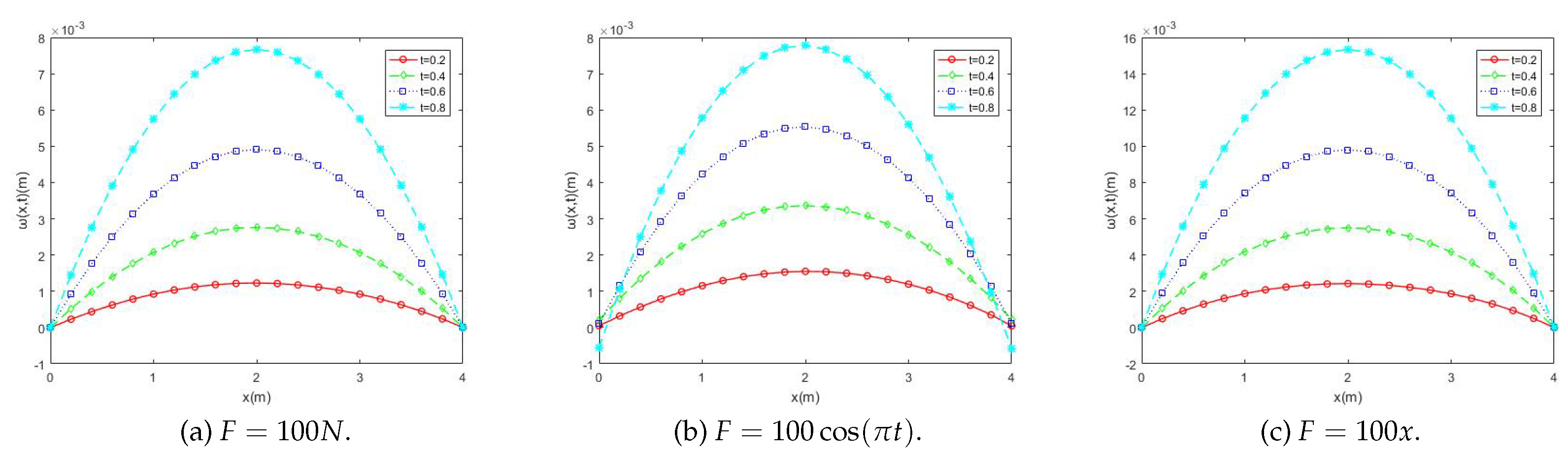
6.2. Displacement Numerical Solution of Viscoelastic Bar

For this example, we consider a bar with a length of $l=4m$, and the associated viscoelastic parameters are listed in

Table 3. Geometrical characteristics and material properties of viscoelastic bar [39].

Parameter	Symbol	Value	Unit
Length	l	4	m
Density	$\rho$	7500	kg/m3
Instant elasticity modulus	$E_1$	2.5 × 105	Pa
Prolonged elasticity modulus	$E_2$	2.5 × 105	Pa

.

A uniform load of $F=100N$, a simple harmonic load of $F=100cos\left(\pi t\right)$, and a linear load of $F=100x$ are applied to the viscoelastic bar, respectively, to find out the corresponding displacements of the bar under different loads, as shown in Figure 3.

The displacement of the viscoelastic bar is maximum at $x=2m$ and the displacement change shows symmetry at this position. As the homogeneous load is applied, the bar’s displacement increases. Furthermore, displacement gradually rises over time under three distinct loading conditions, as determined by assumption; $c_0=1.34\times {10}^{-6} {\mathrm{s}}^{-2}$ and $c_1=1.34\times {10}^{-7} {\mathrm{m}}^{-2}{\mathrm{s}}^{-2}$.

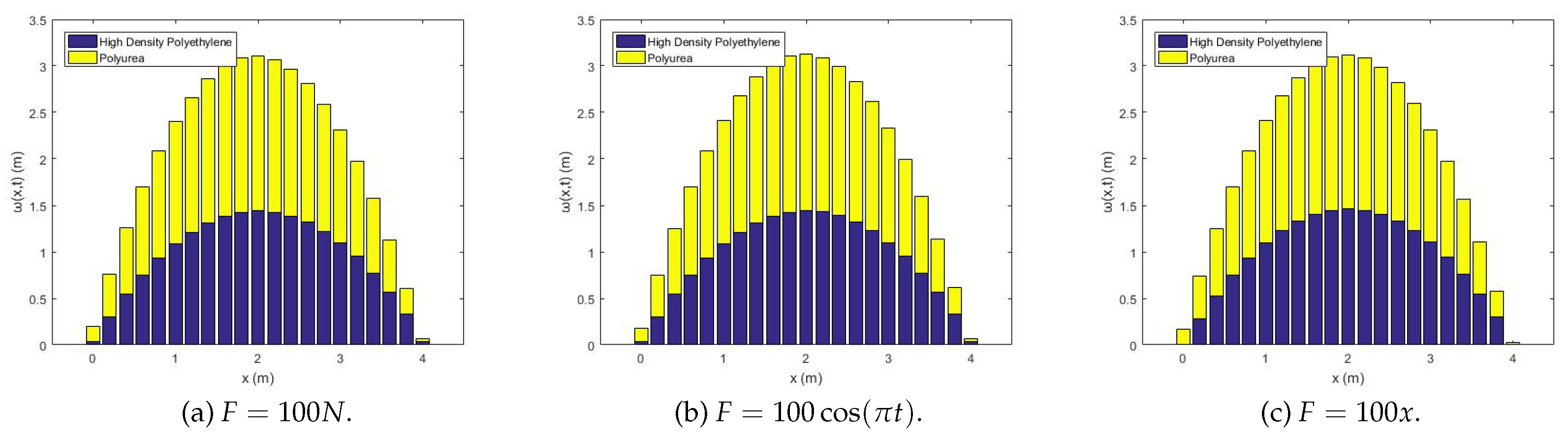
6.3. Displacement Numerical Solutions of HDPE Bar and Polyurea Bar

In this example, two types of viscoelastic bars are considered, high-density polyethylene (HDPE) and polyurea. The material parameters [9] are given in

Table 4. Material parameters of HDPE and polyurea.

Material	$\mathit{\rho }$	${\mathit{E}}_1$	${\mathit{E}}_2$
HDPE	960 kg/m3	8.5 × 106 Pa	8.5 × 106 Pa
Polyurea	1060 kg/m3	1.2 × 107 Pa	1.2 × 107 Pa

.

The influence of materials on viscoelastic bar displacement was analyzed under three types of external forces, including a homogeneous load, a simple harmonic load, and a linear load. Figure 4 shows the displacement of bar HDPE and polyurea at $t=0.6$ s. It is evident that the three displacement solutions for HDPE consistently exceed those of the polyurea material. The displacements of both materials are symmetric around the middle position and zero at both ends. In addition, the displacement of polyurea is lesser than that of HDPE and polyurea has better damping characteristics and greater resistance to bending compared to HDPE. The numerical analysis outcomes produced by this algorithm mirror the intrinsic mechanical behavior of the chosen materials, indicating its effectiveness and reliability in solving the problems related to variable fractional-order viscoelastic variable section bars.

7. Conclusions

In this work, we establish a variable fractional control eaquation to characterize the dynamic behavior of a viscoelastic bar. This is accomplished by integrating a variable fractional constitutive model with the motion equation. To obtain a direct solution in the time domain, we design a numerical approach leveraging shifted Bernstein polynomials. This technique effectively transforms displacement control equations into a linear system by discretizing an differential operator matrix. The developed algorithm provides an in-depth evaluation of the vibration properties of viscoelastic bars, with numerical simulations confirming its precision and reliability. The main findings are outlined as follows:

• Through the introduction of dimensionless equations and a thorough kinetic analysis, it is demonstrated that this approach is highly effective in tackling variable fractional-order differential equations that describe viscoelastic bars.
• When the bar is subjected to different axial loads, uniformly distributed, simple harmonic, and linearly distributed, the displacement increases with both load intensity and time.
• Numerical results illustrate the displacement and stress variations for HDPE and polyurea materials under different loading conditions. Additionally, a comparative analysis of materials with different viscoelastic properties provides theoretical insights into their mechanical behavior.

References

1. Xu, L.; Zhang, J.; Li, J.; Tian, H.; Zheng, C.; Guo, S. Design of a lightweight broadband vibration reduction structure with embedded acoustic black holes in viscoelastic damping materials. Mater. Des. 2024, 248, 113450. [Google Scholar] [CrossRef]
2. Li, F. Incorporating fractional operators into interaction dynamics of a chaotic biological model. Results Phys. 2023, 54, 107052. [Google Scholar] [CrossRef]
3. Chen, J.; Du, C.; Wang, Q.; Peng, X. A 3D finite strain constitutive model for shape memory polymers combined viscoelasticity and storage strain. Mech. Mater. 2024, 197, 105103. [Google Scholar] [CrossRef]
4. Ribeiro, E.A.; de Oliveira Lopes, E.M.; Bavastri, C.A. A numerical and experimental study on optimal design of multi-DOF viscoelastic supports for passive vibration control in rotating machinery. J. Sound Vib. 2017, 411, 346–361. [Google Scholar] [CrossRef]
5. Simoes, R.; Cunha, A.M.; Brostow, W. Computer simulations of true stress development and viscoelastic behavior in amorphous polymeric materials. Comput. Mater. Sci. 2006, 36, 319–328. [Google Scholar] [CrossRef]
6. Carrera, Y.; Avila-de La Rosa, G.; Vernon-Carter, E.; Alvarez-Ramirez, J. A fractional-order Maxwell model for non-Newtonian fluids. Phys. A Stat. Mech. Its Appl. 2017, 482, 276–285. [Google Scholar] [CrossRef]
7. Ren, D.; Shen, X.; Li, C.; Cao, X. The fractional Kelvin-Voigt model for Rayleigh surface waves in viscoelastic FGM infinite half space. Mech. Res. Commun. 2018, 87, 53–58. [Google Scholar] [CrossRef]
8. Lewandowski, R.; Wielentejczyk, P. Nonlinear vibration of viscoelastic beams described using fractional order derivatives. J. Sound Vib. 2017, 399, 228–243. [Google Scholar] [CrossRef]
9. Xu, H.; Jiang, X. Creep constitutive models for viscoelastic materials based on fractional derivatives. Comput. Math. Appl. 2017, 73, 1377–1384. [Google Scholar] [CrossRef]
10. Tarasov, V.E. Generalized memory: Fractional calculus approach. Fractal Fract. 2018, 2, 23. [Google Scholar] [CrossRef]
11. Almeida, R. Functional differential equations involving the ψ-Caputo fractional derivative. Fractal Fract. 2020, 4, 29. [Google Scholar] [CrossRef]
12. Guo, S.; Pu, H.; Yang, M.; Sha, Z.; Liu, D.; Xie, J.; Feng, Y. New perspective on the creep characteristic of fiber–dependent shape memory polymers: Variable–order fractional constitutive model. J. Mater. Res. Technol. 2023, 24, 5177–5185. [Google Scholar]
13. Han, C.; Chen, Y.; Cheng, G.; Serra, R.; Wang, L.; Feng, J. Numerical analysis of axially non-linear viscoelastic string with the variable fractional order model by using Bernstein polynomials algorithm. Int. J. Comput. Math. 2022, 99, 537–552. [Google Scholar] [CrossRef]
14. Cai, W.; Wang, P. Rate-dependent fractional constitutive model for nonlinear behaviors of rubber polymers. Eur. J. Mech.-A/Solids 2024, 103, 105186. [Google Scholar] [CrossRef]
15. Wang, L.; Chen, Y.M. Shifted-Chebyshev-polynomial-based numerical algorithm for fractional order polymer visco-elastic rotating beam. Chaos Solitons Fractals 2020, 132, 109585. [Google Scholar] [CrossRef]
16. Saeed, U.; ur Rehman, M. Haar wavelet Picard method for fractional nonlinear partial differential equations. Appl. Math. Comput. 2015, 264, 310–322. [Google Scholar] [CrossRef]
17. Wang, Y.; Chen, Y. Shifted Legendre Polynomials algorithm used for the dynamic analysis of viscoelastic pipes conveying fluid with variable fractional order model. Appl. Math. Model. 2020, 81, 159–176. [Google Scholar] [CrossRef]
18. Soradi-Zeid, S.; Jahanshahi, H.; Yousefpour, A.; Bekiros, S. King algorithm: A novel optimization approach based on variable-order fractional calculus with application in chaotic financial systems. Chaos Solitons Fractals 2020, 132, 109569. [Google Scholar] [CrossRef]
19. Pezza, L.; Pitolli, F. A multiscale collocation method for fractional differential problems. Math. Comput. Simul. 2018, 147, 210–219. [Google Scholar] [CrossRef]
20. Wang, Y.; Mei, L.; Li, Q.; Bu, L. Split-step spectral Galerkin method for the two-dimensional nonlinear space-fractional Schrödinger equation. Appl. Numer. Math. 2019, 136, 257–278. [Google Scholar] [CrossRef]
21. Yang, Z.; Yuan, Z.; Nie, Y.; Wang, J.; Zhu, X.; Liu, F. Finite element method for nonlinear Riesz space fractional diffusion equations on irregular domains. J. Comput. Phys. 2017, 330, 863–883. [Google Scholar] [CrossRef]
22. Wang, Q. Homotopy perturbation method for fractional KdV-Burgers equation. Chaos Solitons Fractals 2008, 35, 843–850. [Google Scholar] [CrossRef]
23. Odibat, Z.; Momani, S. Application of variational iteration method to nonlinear differential equations of fractional order. Int. J. Nonlinear Sci. Numer. Simul. 2006, 7, 27–34. [Google Scholar] [CrossRef]
24. Ray, S.S.; Bera, R. An approximate solution of a nonlinear fractional differential equation by Adomian decomposition method. Appl. Math. Comput. 2005, 167, 561–571. [Google Scholar]
25. Li, J.; Ahmad, I.; Ahmad, H.; Shah, D.; Chu, Y.-M.; Thounthong, P.; Ayaz, M. Numerical solution of two-term time-fractional PDE models arising in mathematical physics using local meshless method. Open Phys. 2020, 18, 1063–1072. [Google Scholar] [CrossRef]
26. Baleanu, D.; Jassim, H.K. Exact solution of two-dimensional fractional partial differential equations. Fractal Fract. 2020, 4, 21. [Google Scholar] [CrossRef]
27. Wang, L.; Chen, Y.; Cheng, G.; Barrière, T. Numerical analysis of fractional partial differential equations applied to polymeric visco-elastic Euler-Bernoulli beam under quasi-static loads. Chaos Solitons Fractals 2020, 140, 110255. [Google Scholar] [CrossRef]
28. Mei, L.; Wu, B.; Lin, Y. Shifted-Legendre orthonormal method for delay heat conduction equation. Appl. Math. Lett. 2022, 130, 107996. [Google Scholar] [CrossRef]
29. Chouhan, D.; Mishra, V.; Srivastava, H. Bernoulli wavelet method for numerical solution of anomalous infiltration and diffusion modeling by nonlinear fractional differential equations of variable order. Results Appl. Math. 2021, 10, 100146. [Google Scholar] [CrossRef]
30. Feng, Y.; Liu, L.; Chen, Y. Numerical analysis of fractional-order variable section cantilever beams. ICIC Express Lett. 2019, 13, 547–555. [Google Scholar]
31. Kadkhoda, N. A numerical approach for solving variable order differential equations using Bernstein polynomials. Alex. Eng. J. 2020, 59, 3041–3047. [Google Scholar] [CrossRef]
32. Wu, J.; Zhou, Y.; Han, X.; Cheng, S. The blackbody radiation inversion problem: A numerical perspective utilizing Bernstein polynomials. Int. Commun. Heat Mass Transf. 2019, 107, 114–120. [Google Scholar] [CrossRef]
33. Khataybeh, S.N.; Hashim, I.; Alshbool, M. Solving directly third-order ODEs using operational matrices of Bernstein polynomials method with applications to fluid flow equations. J. King Saud Univ. Sci. 2019, 31, 822–826. [Google Scholar] [CrossRef]
34. Ahmad, I.; Alshammari, A.O.; Jan, R.; Razak, N.N.A.; Idris, S.A. An Efficient Numerical Solution of a Multi-Dimensional Two-Term Fractional Order PDE via a Hybrid Methodology: The Caputo–Lucas–Fibonacci Approach with Strang Splitting. Fractal Fract. 2024, 8, 364. [Google Scholar] [CrossRef]
35. Rostamy, D.; Jafari, H.; Alipour, M.; Khalique, C.M. Computational method based on Bernstein operational matrices for multi-order fractional differential equations. Filomat 2014, 28, 591–601. [Google Scholar] [CrossRef]
36. Maleknejad, K.; Hashemizadeh, E.; Basirat, B. Computational method based on Bernstein operational matrices for nonlinear Volterra–Fredholm–Hammerstein integral equations. Commun. Nonlinear Sci. Numer. Simul. 2012, 17, 52–61. [Google Scholar] [CrossRef]
37. Bataineh, A.; Isik, O.; Aloushoush, N.; Shawagfeh, N. Bernstein operational matrix with error analysis for solving high order delay differential equations. Int. J. Appl. Comput. Math. 2017, 3, 1749–1762. [Google Scholar] [CrossRef]
38. Cui, Y.; Qu, J.; Han, C.; Cheng, G.; Zhang, W.; Chen, Y. Shifted Bernstein–Legendre polynomial collocation algorithm for numerical analysis of viscoelastic Euler–Bernoulli beam with variable order fractional model. Math. Comput. Simul. 2022, 200, 361–376. [Google Scholar] [CrossRef]
39. Malara, G.; Pomaro, B.; Spanos, P.D. Nonlinear stochastic vibration of a variable cross-section rod with a fractional derivative element. Int. J. Non-Linear Mech. 2021, 135, 103770. [Google Scholar] [CrossRef]
40. Khan, R.A.; Khalil, H. A new method based on legendre polynomials for solution of system of fractional order partial differential equations. Int. J. Comput. Math. 2014, 91, 2554–2567. [Google Scholar] [CrossRef]
41. Nemati, S.; Ordokhani, Y. Legendre expansion methods for the numerical solution of nonlinear 2D Fredholm integral equations of the second kind. J. Appl. Math. Inform. 2013, 31, 609–621. [Google Scholar] [CrossRef]
Figure 1. Structure of a viscoelastic bar.
Fractalfract 09 00192 g001
Figure 2. Exact solution and numerical solution at different points.
Fractalfract 09 00192 g002
Figure 3. Displacement of different bar loads.
Fractalfract 09 00192 g003
Figure 4. Comparison of displacements of HDPE and polyurea bars under different loads.
Fractalfract 09 00192 g004