Homotopy Analysis Transform Method for Solving Systems of Fractional-Order Partial Differential Equations

Abstract

This paper proposes an innovative method that combines the homotopy analysis method with the Jafari transform, applying it for the first time to solve systems of fractional-order linear and nonlinear differential equations. The method constructs approximate solutions in the form of a series and validates its feasibility through comparison with known exact solutions. The proposed approach introduces a convergence parameter ℏ, which plays a crucial role in adjusting the convergence range of the series solution. By appropriately selecting initial terms, the convergence speed and computational accuracy can be significantly improved. The Jafari transform can be regarded as a generalization of classical transforms such as the Laplace and Elzaki transforms, enhancing the flexibility of the method. Numerical results demonstrate that the proposed technique is computationally efficient and easy to implement. Additionally, when the convergence parameter $\hslash =-1$, both the homotopy perturbation method and the Adomian decomposition method emerge as special cases of the proposed method. The knowledge gained in this study will be important for model solving in the fields of mathematical economics, analysis of biological population dynamics, engineering optimization, and signal processing.

1. Introduction

Fractional-order partial differential equations (FPDEs), as generalizations of integer-order partial differential equations, exhibit unique advantages in characterizing complex phenomena with memory, hereditary effects, and non-local effects. In recent years, with their wide application in fields such as physics, biology, material sciences, and fluid dynamics, the theoretical study of FPDEs has received increasing attention and has gradually developed into an important mathematical tool for solving complex system modeling problems [1,2,3,4]. However, due to the non-local nature of fractional-differential operators, exact solutions can only be obtained in a few cases, and most problems can only be solved approximately. Therefore, knowing how to efficiently solve FPDEs has become a key research focus in the field [5,6,7]. At present, various methods have been developed for solving FPDEs, including the integral transform method [8,9,10], Adomian decomposition method [11], variational iteration method [12,13], homotopy perturbation method [14,15,16], homotopy analysis method (HAM) [17,18,19,20], and homotopy analysis transform method (HATM) [21]. Among these, HATM has been successfully applied to solve many nonlinear problems such as the telegraph equation [22], fractional fisher equation [23], two-dimensional solute transport problem [24], fractional (2 + 1)-D and (3 + 1)-D nonlinear schrödinger equations [25], modified nonlinear KdV equation [26], and so on. In this study, we generalize HATM for the first time to solve a system of fractional-order partial differential equations, as follows:

$$\left\{\begin{array}{c}{\mathcal{D}}_t^{\alpha }\psi (x,y,t)+{\mathcal{A}}_1(\psi (x,y,t),\phi (x,y,t))+{\mathcal{B}}_1(\psi (x,y,t),\phi (x,y,t))=f_1(x,y,t),\hfill \\ {\mathcal{D}}_t^{\alpha }\phi (x,y,t)+{\mathcal{A}}_2(\psi (x,y,t),\phi (x,y,t))+{\mathcal{B}}_2(\psi (x,y,t),\phi (x,y,t))=f_2(x,y,t),\hfill \end{array}\right.$$

(1)

with the initial condition

$$\psi (x,y,0)={\sigma }_1(x,y),\phi (x,y,0)={\sigma }_2(x,y),$$

(2)

where $n-1<\alpha ⩽n$, ${\mathcal{A}}_1,{\mathcal{A}}_2$, and ${\mathcal{B}}_1,{\mathcal{B}}_2$ represent linear and non-linear operators, respectively. The derivative in (1) is the caputo-fractional derivative of $\alpha$-order.

In 2010, Zurigat et al. applied HAM to solve a series of ordinary differential equations [27]. In 2019, Jena et al. solved the Navier–Stokes system of equations using the homotopy perturbation Elzaki transform [28]. Shah et al. utilized the Mohand transform in combination with the Adomian decomposition method to solve a system of fractional-order partial differential equations [29]. In 2020, Khan et al. employed the Laplace–Adomian decomposition method to solve a system of nonlinear fractional-order partial differential equations [30]. Compared with existing methods, we show significant advantages when solving this system of equations by using HATM. We choose the Jafari transform $\mathcal{T}$ as an auxiliary linear operator and construct a recursive formulation of the solution based on suitably chosen initial terms, which simplifies the iterative process. One of the core strengths of HATM in handling nonlinear problems lies in its adjustable convergence control parameter ℏ, which offers a powerful mechanism to ensure the convergence of the series solution [31,32]. Liao provided a more efficient way to identify the optimal convergence parameter ℏ [33]. Notably, when setting $\hslash =-1$, the Adomian decomposition method and the homotopy perturbation method can be viewed as special cases of the proposed method [28,29,34]. To verify the reliability of the proposed technique, its numerical error estimation was analyzed in comparison with the Adomian decomposition method and homotopy perturbation transform method [35]. The technique was further compared with the differential transformation method and finite difference method [24]. The results of the study consistently show that the technique is capable of obtaining analytic solutions with higher accuracy.

The key point of this study is the construction of initial terms in HATM. The selection of the initial term must strictly satisfy the initial and boundary conditions. And, it should be as simple as possible in order to facilitate the computation of higher-order terms. In practical applications, if the initial term deviates significantly from the exact solution, it may lead to a divergence of the series solution. In such cases, adjusting the convergence control parameter ℏ becomes necessary to improve convergence. It should be noted that there are various mature techniques available for optimal selection of the convergence parameter ℏ, for example, the classical value $\hslash =-1$ has a good computing stability. In addition, the study performs stability analysis and provides visualization solutions, which is a significant advancement in the analysis of highly nonlinear models.

The remaining work is designed as follows: In Section 2, we introduce the basic definitions and properties of fractional calculus, Jafafi transform, and the homotopy analysis method. Section 3 presents the specific steps for solving fractional-order partial differential equation systems using HATM. In Section 4, we validate the proposed method with three examples, present solution-related graphs and conduct numerical analysis. Lastly, a conclusion is given in Section 5.

2. Preliminaries

In this section, we introduce the basics of fractional calculus, Jafafi transform, and the homotopy analysis method.

2.1. Basic Definitions Fractional-Calculus Operators

Definition 1

([36]). The α-order integral of $f\left(t\right)$ is defined as

$${\mathcal{J}}_{\mathrm{t}}^{-\alpha }f\left(t\right)={\displaystyle \frac{1}{\Gamma \left(\alpha \right)}}{\int }_0^t{(t-\tau )}^{\alpha -1}f\left(t\right)d\tau .$$

(3)

where $\alpha >0$.

Definition 2

([37]). The Riemann–Liouville fractional derivative of $f\left(t\right)$ is defined as

$${}^{\mathit{RL}}\mathcal{D}_t^{\alpha }f\left(t\right)={\displaystyle \frac{1}{\Gamma (n-\alpha )}}{\displaystyle \frac{d^n}{d{t}^n}}{\int }_0^t{\displaystyle \frac{f\left(\tau \right)}{{(t-\tau )}^{\alpha -n+1}}}d\tau ,$$

(4)

where $n-1\le \alpha <n$, $n\in {\mathbb{Z}}^{+}$.

Definition 3

([38]). The Caputo fractional derivative of $f\in {\mathcal{C}}_{-1}^n$ is defined as

$${}^C\mathcal{D}_t^{\alpha }f\left(t\right)={\displaystyle \frac{1}{\Gamma (n-\alpha )}}{\int }_0^t{\displaystyle \frac{f^{\left(n\right)}\left(\tau \right)}{{(t-\tau )}^{\alpha -n+1}}}d\tau ,$$

(5)

where $n-1<\alpha \le n$, $n\in \mathbb{N}$.

2.2. Basic Definitions and Properties of Jafrai Transform

Definition 4

([39]). The Jafari transform of a given function $f\left(t\right)$ is defined as

$$\mathcal{T}\{f\left(t\right);s\}=\mathcal{F}\left(s\right)=p\left(s\right){\int }_0^{\infty }f\left(t\right)e^{-q\left(s\right)t}dt,$$

(6)

where $t\ge 0,p\left(s\right)\ne 0$, and $q\left(s\right)$ are positive real functions.

Proof. 

For all $t\ge 0$, the function $f\left(t\right)$ is a piecewise continuous function of an exponential order and satisfies $\left|f\left(t\right)\right|\le M{e}^{kt}$, then $\mathcal{F}\left(s\right)$ exists for all $Re\left(q\right(s\left)\right)>k$, where M and k are both positive constants.

$$\begin{array}{cc}\hfill \left|\mathcal{T}\left\{f\left(t\right);s\right\}\right|& =\left|p\left(s\right){\int }_0^{\infty }f\left(t\right)e^{-q\left(s\right)t}dt\right|\le \left|p\left(s\right)\right|{\int }_0^{\infty }\left|f\left(t\right)\right|e^{-q\left(s\right)t}dt\hfill \\ & \le \left|p\left(s\right)\right|{\int }_0^{\infty }M{e}^{kt}{e}^{-q\left(s\right)t}dt\le {\displaystyle \frac{M\left|p\left(s\right)\right|}{q^{\left(s\right)-k}}},\hfill \end{array}$$

the statement is valid. □

Some basic properties

• The Jafari transform of the Riemann–Liouville fractional derivative $f\left(t\right)$ is represented as

  $$\mathcal{T}\left[{}^{\mathit{RL}}\mathcal{D}_t^{\alpha }f\left(t\right)\right]=q^{\alpha }\left(s\right)\mathcal{F}\left(s\right)-p\left(s\right)\sum _{k=0}^{n-1}{q}^k\left(s\right){\mathcal{J}}^{\alpha -k-1}f\left(0\right),(n-1<\alpha \le n).$$

  (7)

• The Jafari transform of the Caputo fractional derivative $f\left(t\right)$ is represented as

  $$\mathcal{T}\left[{}^C\mathcal{D}_t^{\alpha }f\left(t\right)\right]=q^{\alpha }\left(s\right)\mathcal{F}\left(s\right)-\sum _{k=0}^{n-1}{q}^{\alpha -1-k}\left(s\right)p\left(s\right)f^{\left(k\right)}\left(0\right),(n-1<\alpha \le n).$$

  (8)

• The Jafari transform of certain partial derivatives is represented as

  $$\begin{array}{cc}\hfill & \left(a\right)\mathcal{T}\left[{\displaystyle \frac{\partial f(x,t)}{\partial t}}\right]=q\left(s\right)\mathcal{F}(x,s)-p\left(s\right)f(x,0).\hfill \end{array}$$

  (9)

  $$\begin{array}{cc}\hfill & \left(b\right)\mathcal{T}\left[{\displaystyle \frac{{\partial }^{2}f(x,t)}{\partial t^2}}\right]=q^2\left(s\right)\mathcal{F}(x,s)-q\left(s\right)p\left(s\right)f(x,0)-p\left(s\right){\displaystyle \frac{\partial f(x,0)}{\partial t}}.\hfill \end{array}$$

  (10)

  $$\begin{array}{cc}\hfill & \left(c\right)\mathcal{T}\left[{\displaystyle \frac{\partial f(x,t)}{\partial x}}\right]={\displaystyle \frac{d}{dx}}\left[\mathcal{F}(x,s)\right].\hfill \end{array}$$

  (11)

  $$\begin{array}{cc}\hfill & \left(d\right)\mathcal{T}\left[{\displaystyle \frac{{\partial }^{2}f(x,t)}{\partial x^2}}\right]={\displaystyle \frac{d^2}{d{x}^2}}\left[\mathcal{F}(x,s)\right].\hfill \end{array}$$

  (12)

• The Jafari transform of certain functions is provided

  $$\begin{array}{cc}\hfill & \mathcal{T}\left[1\right]={\displaystyle \frac{p\left(s\right)}{q\left(s\right)}},\mathcal{T}\left[t\right]={\displaystyle \frac{p\left(s\right)}{q^2\left(s\right)}},\mathcal{T}\left[{\displaystyle \frac{t^{\alpha }}{\Gamma (\alpha +1)}}\right]={\displaystyle \frac{p\left(s\right)}{q^{\alpha +1}\left(s\right)}},\hfill \\ \hfill & \mathcal{T}\left[sint\right]={\displaystyle \frac{p\left(s\right)}{q^2\left(s\right)+1}},\mathcal{T}\left[e^{at}\right]={\displaystyle \frac{p\left(s\right)}{q\left(s\right)-a}},\mathcal{T}\left[f^{\prime }\left(t\right)\right]=q\left(s\right)\mathcal{T}\left(s\right)-p\left(s\right)f\left(0\right).\hfill \end{array}$$

2.3. The Definition and Procedure of Homotopy Analysis

Homotopy analysis is an analytical approach to nonlinear problems that can be used effectively to solve nonlinear differential equation and partial differential equation problems. By constructing a homotopy transformation, the nonlinear problem can be transformed into a series of linear problems, and its solution can be approached step by step. Assuming that the nonlinear differential equation is

$$\mathcal{N}\left[u\right(x,t\left)\right]=0,$$

(13)

where $\mathcal{N}$ is a nonlinear operator.

By introducing an embedding parameter $q(0\le q\le 1)$, an auxiliary linear operator $\mathcal{T}$, an initial guess solution $u_0(x,t)$, and a convergence parameter ℏ, we can construct a zero-order deformation equation, i.e.,

$$(1-q)\mathcal{T}\left[\varphi (x,t;q)-u_0(x,t)\right]=q\hslash \mathcal{N}\left[\varphi (x,t;q)\right].$$

(14)

When $q=0$, Equation (14) becomes

$$\mathcal{T}\left[\varphi (x,t;q)-u_0(x,t)\right]=0.$$

(15)

According to the properties of the auxiliary linear operator, the initial guess solution can be obtained

$$\varphi (x,t;0)=u_0(x,t).$$

(16)

When $q=1$, Equation (14) becomes

$$\mathcal{N}\left[\varphi \right(x,t;1\left)\right]=0.$$

(17)

The solution to the original nonlinear problem is

$$\varphi (x,t;1)=u(x,t).$$

(18)

The homotopy function $\varphi (x,t;q)$ is expanded into a power series, i.e.,

$$\varphi (x,t;q)=\sum _{m=0}^{\infty }{u}_m(x,t)q^m.$$

(19)

The power series (19) converges when $q=1$ by selecting the correct auxiliary linear operator, initial guess solution, and covergence ℏ parameter, and we have

$$u(x,t)=\sum _{m=0}^{\infty }{u}_m(x,t).$$

(20)

We define the vectors $\overrightarrow{u_m}=\left\{u_0(x,t),u_1(x,t),\dots ,u_m(x,t)\right\}$. Taking the m- times derivative of (14) with respect to q and dividing it by m!. Finally, setting $q=0$, we obtain the following m-order deformation equation

$$\mathcal{T}\left[u_m(x,t)-{\chi }_m{u}_{m-1}(x,t)\right]=\hslash {\mathcal{R}}_m\left(\overrightarrow{u_{m-1}}(x,t)\right),$$

(21)

where

$${\mathcal{R}}_m\left(\overrightarrow{u_{m-1}}(x,t)\right)={\displaystyle \frac{1}{(m-1)!}}{\displaystyle \frac{{\partial }^{m-1}\mathcal{N}\left[\varphi (x,t;q)\right]}{\partial q^{m-1}}}{|}_{q=0},$$

(22)

and

$${\chi }_m=\left\{\begin{array}{ccc}0,\hfill & \hfill & m\le 1,\hfill \\ 1,\hfill & \hfill & m>1.\hfill \end{array}\right.$$

(23)

Solving Equation (21) in turn for $u_1(x,t),u_2(x,t),\dots ,u_m(x,t)$, an approximate solution to the original equation can be found from Equation (20).

3. Homotopy Analysis Transform Method to Solve the System of Equations

In this section, we give specific steps for solving (1) using the homotopy analysis transform method.

Firstly, taking the Jafari transform $\mathcal{T}$ as an auxiliary linear operator and applying it to both sides of (1), i.e.,

$$\left\{\begin{array}{c}\mathcal{T}\left[{\mathcal{D}}_t^{\alpha }\psi (x,y,t)\right]=\mathcal{T}\left[f_1(x,y,t)-{\mathcal{A}}_1(\psi (x,y,t),\phi (x,y,t))-{\mathcal{B}}_1(\psi (x,y,t),\phi (x,y,t))\right],\hfill \\ \mathcal{T}\left[{\mathcal{D}}_t^{\alpha }\phi (x,y,t)\right]=\mathcal{T}\left[f_2(x,y,t)-{\mathcal{A}}_2(\psi (x,y,t),\phi (x,y,t))-{\mathcal{B}}_2(\psi (x,y,t),\phi (x,y,t))\right].\hfill \end{array}\right.$$

(24)

Applying the property (8), we have

$$\left\{\begin{array}{c}\begin{array}{cc}\hfill q^{\alpha }\left(s\right)\mathcal{T}\left[\psi (x,y,t)\right]& -\sum _{k=0}^{n-1}{q}^{\alpha -1-k}\left(s\right)p\left(s\right)\left({\psi }_t^{\left(k\right)}(x,y,0)\right)\hfill \\ & =\mathcal{T}\left[f_1(x,y,t)-{\mathcal{A}}_1(\psi (x,y,t),\phi (x,y,t))-{\mathcal{B}}_1(\psi (x,y,t),\phi (x,y,t))\right],\hfill \end{array}\hfill \\ \begin{array}{cc}\hfill q^{\alpha }\left(s\right)\mathcal{T}\left[\phi (x,y,t)\right]& -\sum _{k=0}^{n-1}{q}^{\alpha -1-k}\left(s\right)p\left(s\right)\left({\phi }_t^{\left(k\right)}(x,y,0)\right)\hfill \\ & =\mathcal{T}\left[f_2(x,y,t)-{\mathcal{A}}_2(\psi (x,y,t),\phi (x,y,t))-{\mathcal{B}}_2(\psi (x,y,t),\phi (x,y,t))\right].\hfill \end{array}\hfill \end{array}\right.$$

(25)

Re-writing (25), we have

$$\left\{\begin{array}{c}\begin{array}{cc}\hfill \mathcal{T}\left[\psi (x,y,t)\right]& =\sum _{k=0}^{n-1}{q}^{-1-k}\left(s\right)p\left(s\right)\left({\psi }_t^{\left(k\right)}(x,y,0)\right)\hfill \\ & + q^{-\alpha }\left(s\right)\mathcal{T}\left[f_1(x,y,t)-{\mathcal{A}}_1(\psi (x,y,t),\phi (x,y,t))-{\mathcal{B}}_1(\psi (x,y,t),\phi (x,y,t))\right],\hfill \end{array}\hfill \\ \begin{array}{cc}\hfill \mathcal{T}\left[\phi (x,y,t)\right]& =\sum _{k=0}^{n-1}{q}^{-1-k}\left(s\right)p\left(s\right)\left({\phi }_t^{\left(k\right)}(x,y,0)\right)\hfill \\ & + q^{-\alpha }\left(s\right)\mathcal{T}\left[f_2(x,y,t)-{\mathcal{A}}_2(\psi (x,y,t),\phi (x,y,t))-{\mathcal{B}}_2(\psi (x,y,t),\phi (x,y,t))\right].\hfill \end{array}\hfill \end{array}\right.$$

(26)

The nonlinear operator $\mathcal{N}$ can be defined as

$$\left\{\begin{array}{c}\begin{array}{cc}\hfill \mathcal{N}\left[{\varphi }_1(x,y,t;q)\right]=& \mathcal{T}\left[{\varphi }_1(x,y,t;q)\right]-\sum _{k=0}^{n-1}{q}^{-1-k}\left(s\right)p\left(s\right)\left({\psi }_t^{\left(k\right)}(x,y,0)\right)-q^{-\alpha }\left(s\right)\mathcal{T}\left[f_1(x,y,t)\right.\hfill \\ \hfill & \left.- {\mathcal{A}}_1({\varphi }_1(x,y,t;q),{\varphi }_2(x,y,t;q))-{\mathcal{B}}_1({\varphi }_1(x,y,t;q),{\varphi }_2(x,y,t;q))\right],\hfill \end{array}\hfill \\ \begin{array}{cc}\hfill \mathcal{N}\left[{\varphi }_2(x,y,t;q)\right]=& \mathcal{T}\left[{\varphi }_2(x,y,t;q)\right]-\sum _{k=0}^{n-1}{q}^{-1-k}\left(s\right)p\left(s\right)\left({\phi }_t^{\left(k\right)}(x,y,0)\right)-q^{-\alpha }\left(s\right)\mathcal{T}\left[f_2(x,y,t)\right.\hfill \\ \hfill & \left.- {\mathcal{A}}_2({\varphi }_1(x,y,t;q),{\varphi }_2(x,y,t;q))-{\mathcal{B}}_2({\varphi }_1(x,y,t;q),{\varphi }_2(x,y,t;q))\right],\hfill \end{array}\hfill \end{array}\right.$$

(27)

where $\varphi (x,y,t;q)$ is a function of $x,y,t,q$ and $q\in [0,1]$. Expanding $\varphi (x,y,t;q)$ into a Taylor series about the embedded variable q, we have

$$\left\{\begin{array}{c}\begin{array}{c}\hfill {\varphi }_1(x,y,t;q)={\psi }_0(x,y,t)+\sum _{m=1}^{\infty }{\psi }_m(x,y,t)q^m,\end{array}\hfill \\ \begin{array}{c}\hfill {\varphi }_2(x,y,t;q)={\phi }_0(x,y,t)+\sum _{m=1}^{\infty }{\phi }_m(x,y,t)q^m,\end{array}\hfill \end{array}\right.$$

(28)

where

$$\left\{\begin{array}{c}\begin{array}{c}\hfill {\psi }_m(x,y,t)={\displaystyle \frac{1}{m!}}{\displaystyle \frac{{\partial }^m{\varphi }_1(x,t;q)}{\partial q^m}}{|}_{q=0},\end{array}\hfill \\ \begin{array}{c}\hfill {\phi }_m(x,y,t)={\displaystyle \frac{1}{m!}}{\displaystyle \frac{{\partial }^m{\varphi }_2(x,t;q)}{\partial q^m}}{|}_{q=0}.\end{array}\hfill \end{array}\right.$$

(29)

We define the zero-order deformation equation

$$\left\{\begin{array}{c}(1-q)\mathcal{T}\left[{\varphi }_1(x,y,t;q)-{\psi }_0(x,y,t)\right]=q\hslash \mathcal{N}\left[{\varphi }_1(x,y,t;q)\right],\hfill \\ (1-q)\mathcal{T}\left[{\varphi }_2(x,y,t;q)-{\phi }_0(x,y,t)\right]=q\hslash \mathcal{N}\left[{\varphi }_2(x,y,t;q)\right],\hfill \end{array}\right.$$

(30)

Then, taking the m-times derivative of (30) with respect to the q and dividing by m!. Finally, we derive the deformation equation of m-order as follows for $q=0$, i.e.,

$$\left\{\begin{array}{c}\mathcal{T}\left[{\psi }_m(x,y,t)-{\chi }_m{\psi }_{m-1}(x,y,t)\right]=\hslash {\mathcal{R}}_m\left(\overrightarrow{{\psi }_{m-1}}(x,y,t)\right),\hfill \\ \mathcal{T}\left[{\phi }_m(x,y,t)-{\chi }_m{\phi }_{m-1}(x,y,t)\right]=\hslash {\mathcal{R}}_m\left(\overrightarrow{{\phi }_{m-1}}(x,y,t)\right),\hfill \end{array}\right.$$

(31)

with

$$\left\{\begin{array}{c}\begin{array}{c}\hfill {\mathcal{R}}_m\left(\overrightarrow{{\psi }_{m-1}}(x,y,t)\right)={\displaystyle \frac{1}{(m-1)!}}{\displaystyle \frac{{\partial }^{m-1}\mathcal{N}\left[{\varphi }_1(x,y,t;q)\right]}{\partial q^{m-1}}}{|}_{q=0},\end{array}\hfill \\ \begin{array}{c}\hfill {\mathcal{R}}_m\left(\overrightarrow{{\phi }_{m-1}}(x,y,t)\right)={\displaystyle \frac{1}{(m-1)!}}{\displaystyle \frac{{\partial }^{m-1}\mathcal{N}\left[{\varphi }_2(x,y,t;q)\right]}{\partial q^{m-1}}}{|}_{q=0},\end{array}\hfill \end{array}\right.$$

(32)

and

$${\chi }_m=\left\{\begin{array}{ccc}0,\hfill & \hfill & m\le 1,\hfill \\ 1,\hfill & \hfill & m>1.\hfill \end{array}\right.$$

(33)

Applying the inverse of the Jafari transform on both sides of (31), we obtain

$$\left\{\begin{array}{c}\begin{array}{cc}\hfill {\psi }_m(x,y,t)={\chi }_m{\psi }_{m-1}(x,y,t)+\hslash {\mathcal{T}}^{-1}\left[{\mathcal{R}}_m\left(\overrightarrow{{\psi }_{m-1}}(x,y,t)\right)\right],& m⩾1,\hfill \end{array}\hfill \\ \begin{array}{cc}\hfill {\phi }_m(x,y,t)={\chi }_m{\phi }_{m-1}(x,y,t)+\hslash {\mathcal{T}}^{-1}\left[{\mathcal{R}}_m\left(\overrightarrow{{\phi }_{m-1}}(x,y,t)\right)\right],& m⩾1.\hfill \end{array}\hfill \end{array}\right.$$

(34)

The approximate solution to the system of equations is found by choosing a suitable initial term and convergence parameter, when (28) converges at $q=1$, i.e.,

$$\left\{\begin{array}{c}\begin{array}{c}\hfill \psi (x,y,t)={\varphi }_1(x,y,t;1)=\sum _{m=0}^{\infty }{\psi }_m(x,y,t),\end{array}\hfill \\ \begin{array}{c}\hfill \phi (x,y,t)={\varphi }_2(x,y,t;1)=\sum _{m=0}^{\infty }{\phi }_m(x,y,t).\end{array}\hfill \end{array}\right.$$

(35)

When $p\left(s\right),q\left(s\right)$ in (27) take on different values, the combination of the homotopy analysis method and Jafari transform can be transformed into the combination of the homotopy analysis method and Laplace, Elzaki, Aboodh, Pourreza, Sumudu, Sawi, Kamal, G, Mohand transforms. The nonlinear operator $\mathcal{N}$ is constructed as shown in

Table 1. The construction of the nonlinear operator $\mathcal{N}$ by combining homotopy analysis with various integral transforms.

Homotopy Analysis Method with Integral Transform	Nonlinear Operator $\mathcal{N}$
Jafari transform	$\mathcal{N}\left[\varphi (x,y,t;q)\right]=\mathcal{T}\left[\varphi (x,y,t;q)\right]-{\sum }_{k=0}^{n-1}{q}^{-1-k}\left(s\right)p\left(s\right)\left(u_t^{\left(k\right)}(x,y,0)\right)-q^{-\alpha }\left(s\right)\mathcal{T}\left[f(x,y,t)-\mathcal{A}\left(\varphi \right(x,y,t;q\left)\right)-\mathcal{B}\left(\varphi \right(x,y,t;q)\right]$
Laplace transform	$\mathcal{N}\left[\varphi \right]=\mathcal{L}\left[\varphi \right]-{\sum }_{k=0}^{n-1}{s}^{-1-k}\left(u_t^{\left(k\right)}(x,y,0)\right)-s^{-\alpha }\left(s\right)\mathcal{L}\left[f-\mathcal{A}\left(\varphi \right)-\mathcal{B}\left(\varphi \right)\right]$
Elzaki transform	$\mathcal{N}\left[\varphi \right]=\mathcal{E}\left[\varphi \right]-{\sum }_{k=0}^{n-1}{s}^{2+k}\left(u_t^{\left(k\right)}(x,y,0)\right)-s^{\alpha }\left(s\right)\mathcal{E}\left[f-\mathcal{A}\left(\varphi \right)-\mathcal{B}\left(\varphi \right)\right]$
Aboodh transform	$\mathcal{N}\left[\varphi \right]=\mathcal{A}\left[\varphi \right]-{\sum }_{k=0}^{n-1}{s}^{-2-k}\left(u_t^{\left(k\right)}(x,y,0)\right)-s^{-\alpha }\left(s\right)\mathcal{A}\left[f-\mathcal{A}\left(\varphi \right)-\mathcal{B}\left(\varphi \right)\right]$
Pourreza transform	$\mathcal{N}\left[\varphi \right]=\mathcal{H}J\left[\varphi \right]-{\sum }_{k=0}^{n-1}{s}^{-1-2k}\left(u_t^{\left(k\right)}(x,y,0)\right)-s^{-2\alpha }\left(s\right)\mathcal{H}J\left[f-\mathcal{A}\left(\varphi \right)-\mathcal{B}\left(\varphi \right)\right]$
Sumudu transform	$\mathcal{N}\left[\varphi \right]=\mathcal{S}\left[\varphi \right]-{\sum }_{k=0}^{n-1}{s}^k\left(u_t^{\left(k\right)}(x,y,0)\right)-s^{\alpha }\left(s\right)\mathcal{S}\left[f-\mathcal{A}\left(\varphi \right)-\mathcal{B}\left(\varphi \right)\right]$
Sawi transform	$\mathcal{N}\left[\varphi \right]={\mathcal{S}}_{⊣}\left[\varphi \right]-{\sum }_{k=0}^{n-1}{s}^{-1-k}\left(u_t^{\left(k\right)}(x,y,0)\right)-s^{\alpha }\left(s\right){\mathcal{S}}_{⊣}\left[f-\mathcal{A}\left(\varphi \right)-\mathcal{B}\left(\varphi \right)\right]$
Kamal transform	$\mathcal{N}\left[\varphi \right]=\mathcal{K}\left[\varphi \right]-{\sum }_{k=0}^{n-1}{s}^{-k}\left(u_t^{\left(k\right)}(x,y,0)\right)-s^{\alpha }\left(s\right){\mathcal{S}}_{⊣}\left[f-\mathcal{A}\left(\varphi \right)-\mathcal{B}\left(\varphi \right)\right]$
G transform	$\mathcal{N}\left[\varphi \right]=\mathcal{G}\left[\varphi \right]-{\sum }_{k=0}^{n-1}{s}^{\alpha +1+k}\left(u_t^{\left(k\right)}(x,y,0)\right)-s^{\alpha }\left(s\right)\mathcal{G}\left[f-\mathcal{A}\left(\varphi \right)-\mathcal{B}\left(\varphi \right)\right]$
Mohand transform	$\mathcal{N}\left[\varphi \right]=\mathcal{M}\left[\varphi \right]-{\sum }_{k=0}^{n-1}{s}^{1-k}\left(u_t^{\left(k\right)}(x,y,0)\right)-s^{-\alpha }\left(s\right)\mathcal{M}\left[f-\mathcal{A}\left(\varphi \right)-\mathcal{B}\left(\varphi \right)\right]$

.

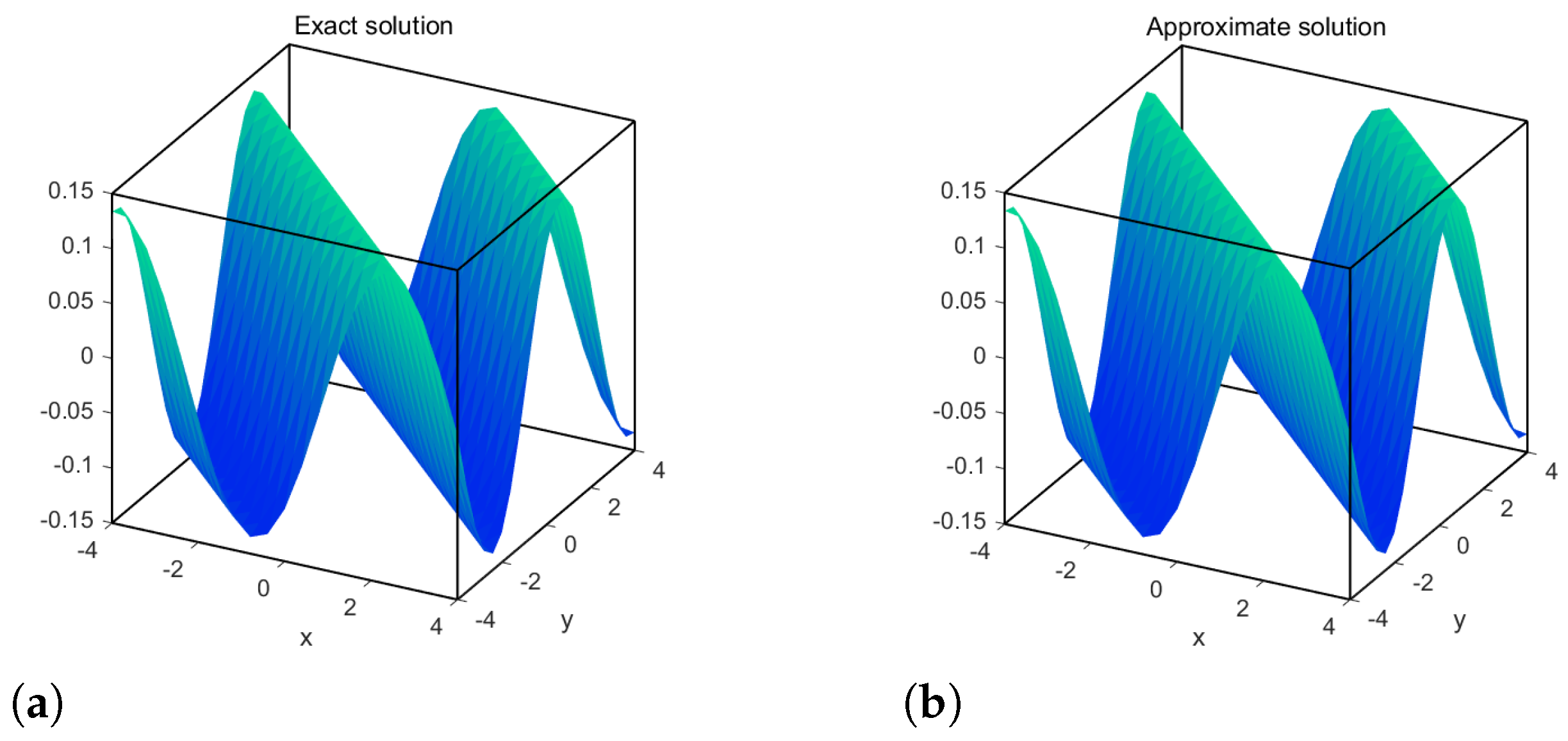
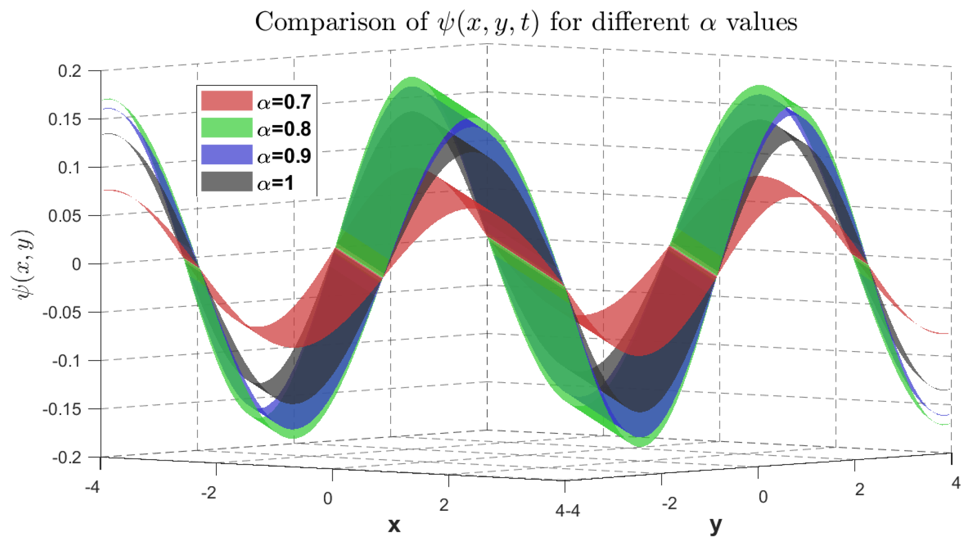
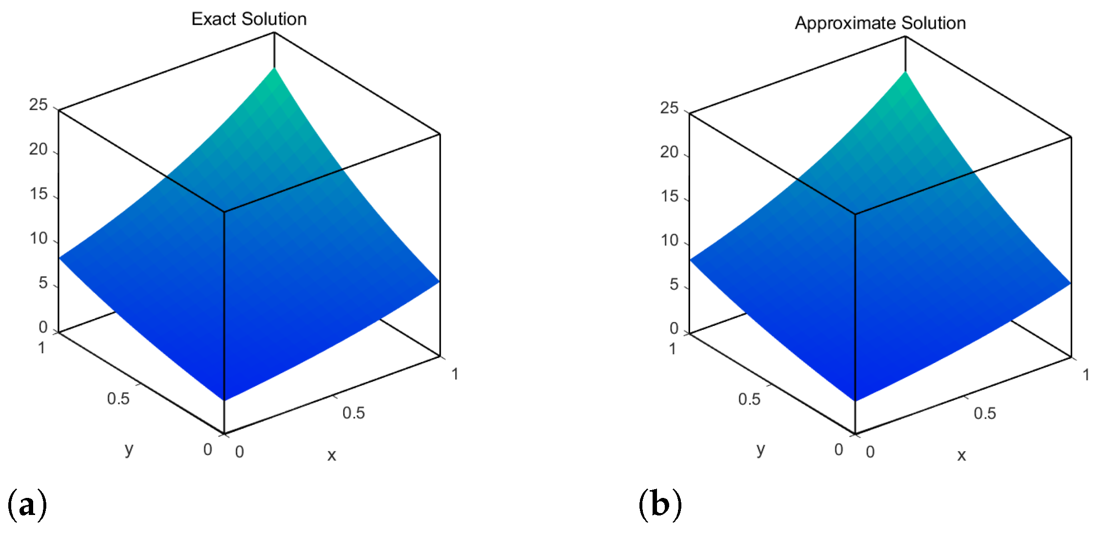
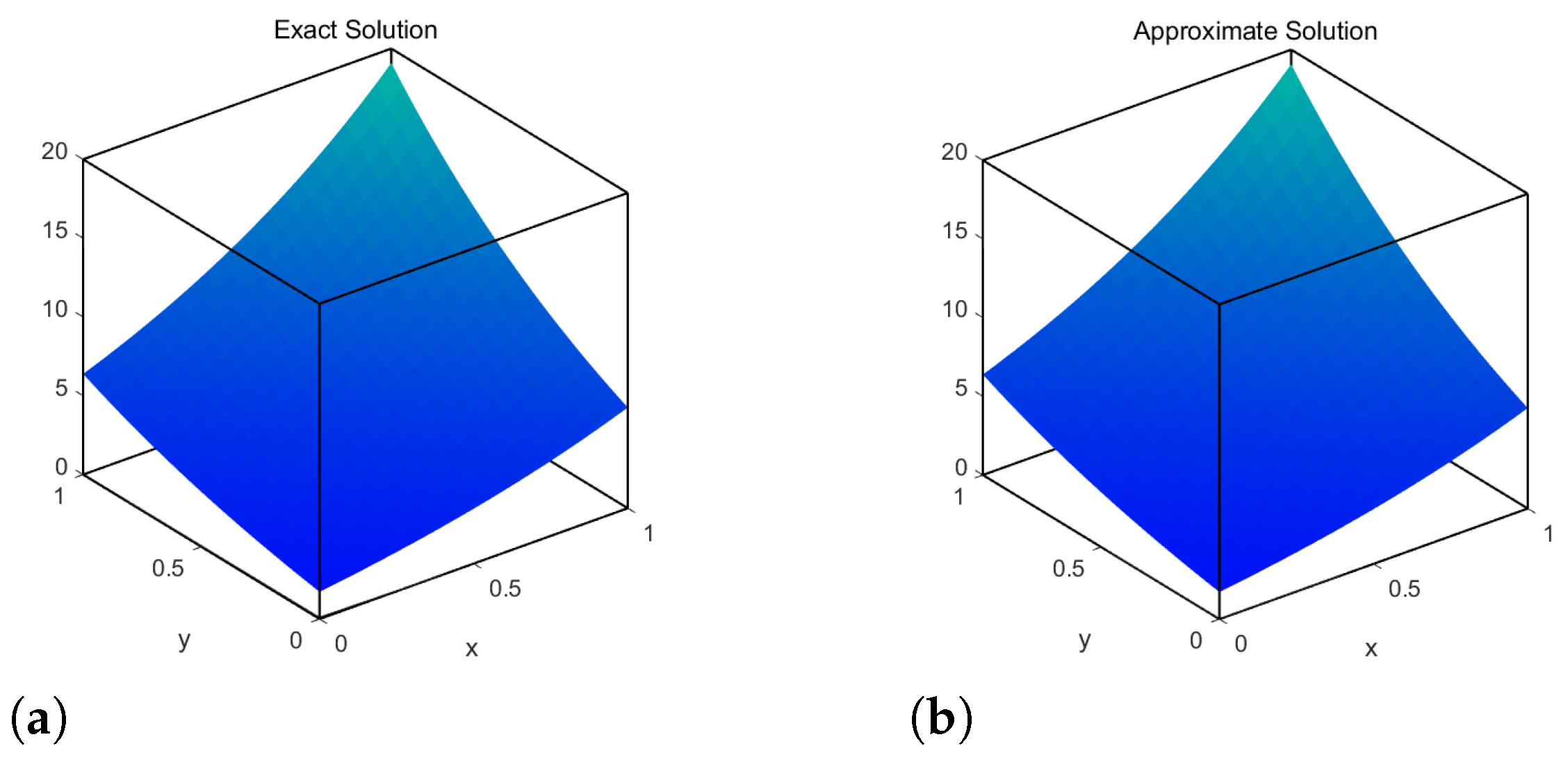
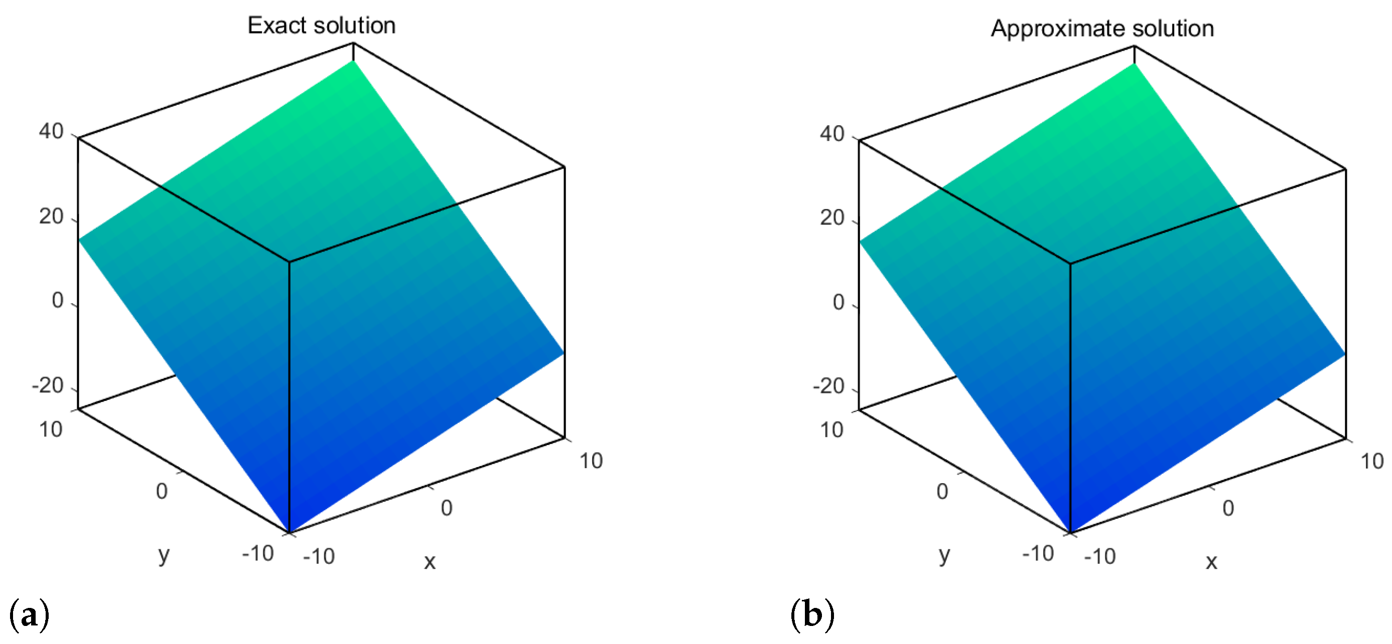
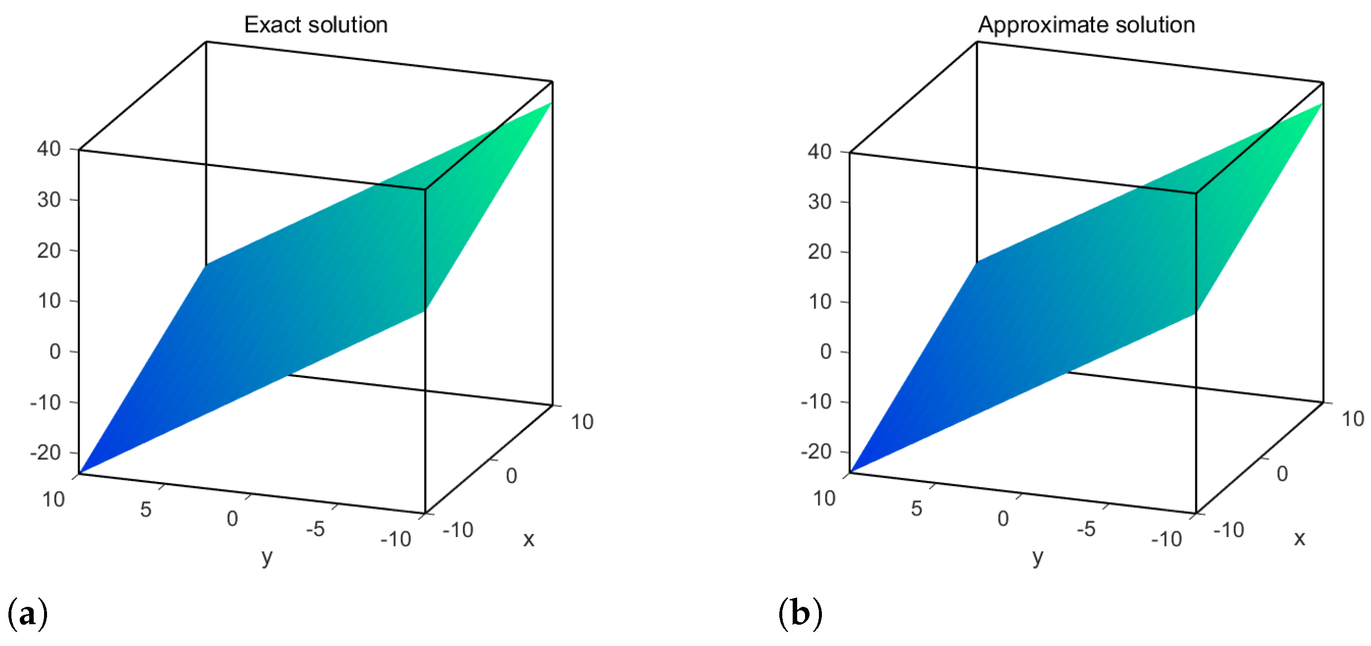
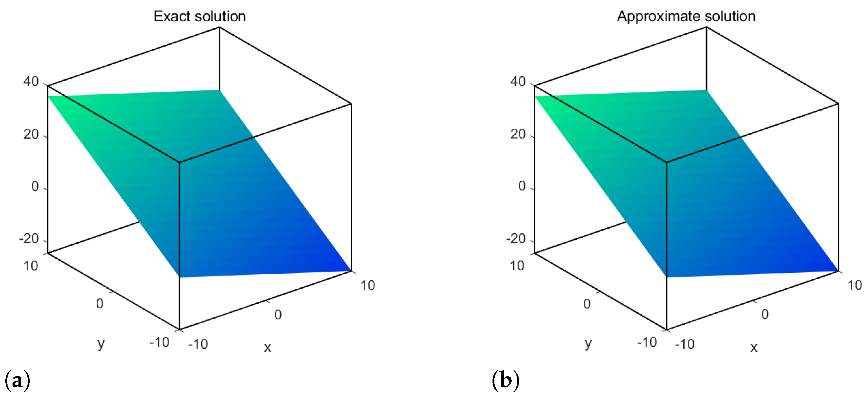
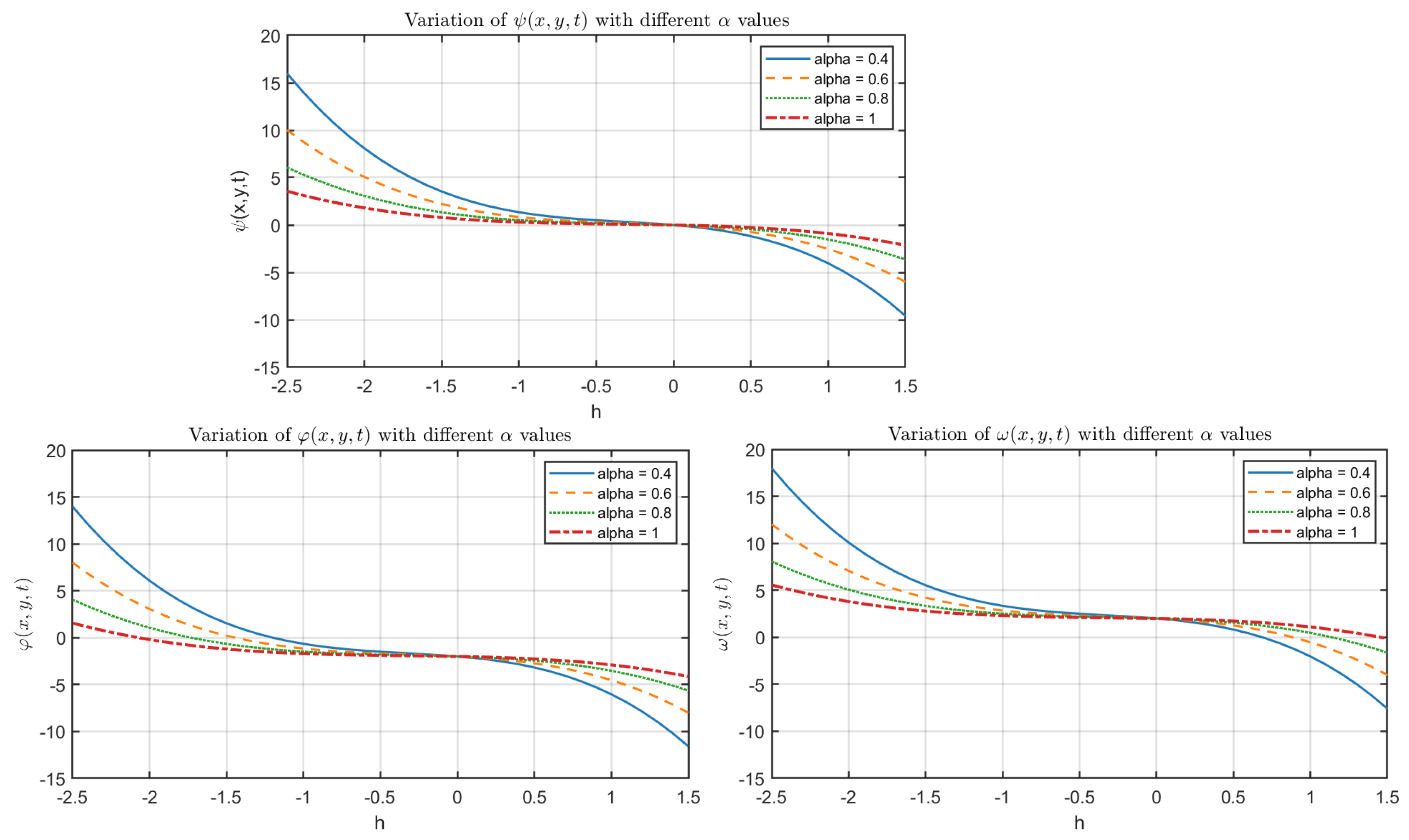
4. Numerical Examples

This section applies the aforementioned numerical methods to perform specific numerical calculations, and the effectiveness, accuracy, and computational precision of the constructed methods in solving linear and nonlinear systems of partial differential equations of a fractional-order are verified by examples.

Example 1.

Consider the nonlinear system of FPDEs from [40]

$$\left\{\begin{array}{c}\begin{array}{c}\hfill {\mathcal{D}}_t^{\alpha }\psi (x,y,t)+\psi (x,y,t){\displaystyle \frac{\partial \psi (x,y,t)}{\partial x}}+\phi (x,y,t){\displaystyle \frac{\partial \psi (x,y,t)}{\partial y}}={\displaystyle \frac{{\partial }^2\psi (x,y,t)}{\partial x^2}}+{\displaystyle \frac{{\partial }^2\psi (x,y,t)}{\partial y^2}},\end{array}\hfill \\ \begin{array}{c}\hfill {\mathcal{D}}_t^{\alpha }\phi (x,y,t)+\psi (x,y,t){\displaystyle \frac{\partial \phi (x,y,t)}{\partial x}}+\phi (x,y,t){\displaystyle \frac{\partial \phi (x,y,t)}{\partial y}}={\displaystyle \frac{{\partial }^2\phi (x,y,t)}{\partial x^2}}+{\displaystyle \frac{{\partial }^2\phi (x,y,t)}{\partial y^2}},\end{array}\hfill \end{array}\right.$$

(36)

where $0<\alpha \le 1$, with initial condition

$$\psi (x,y,0)=-sin(x+y),\phi (x,y,0)=sin(x+y).$$

(37)

Taking the Jafari transform from (36), we obtain

$$\left\{\begin{array}{c}\begin{array}{c}\hfill \mathcal{T}\left[{\mathcal{D}}_t^{\alpha }\psi (x,y,t)\right]=\mathcal{T}\left[{\displaystyle \frac{{\partial }^2\psi }{\partial x^2}}+{\displaystyle \frac{{\partial }^2\psi }{\partial y^2}}-\psi {\displaystyle \frac{\partial \psi }{\partial x}}-\phi {\displaystyle \frac{\partial \psi }{\partial y}}\right],\end{array}\hfill \\ \begin{array}{c}\hfill \mathcal{T}\left[{\mathcal{D}}_t^{\alpha }\phi (x,y,t)\right]=\mathcal{T}\left[{\displaystyle \frac{{\partial }^2\phi }{\partial x^2}}+{\displaystyle \frac{{\partial }^2\phi }{\partial y^2}}-\psi {\displaystyle \frac{\partial \phi }{\partial x}}-\phi {\displaystyle \frac{\partial \phi }{\partial y}}\right].\end{array}\hfill \end{array}\right.$$

(38)

Applying the transform property, we have

$$\left\{\begin{array}{c}\begin{array}{cc}\hfill q^{\alpha }\left(s\right)\mathcal{T}\left[\psi (x,y,t)\right]& - q^{\alpha -1}\left(s\right)p\left(s\right)\left(\psi (x,y,0)\right)\hfill \\ & =\mathcal{T}\left[{\displaystyle \frac{{\partial }^2\psi }{\partial x^2}}+{\displaystyle \frac{{\partial }^2\psi }{\partial y^2}}-\psi {\displaystyle \frac{\partial \psi }{\partial x}}-\phi {\displaystyle \frac{\partial \psi }{\partial y}}\right],\hfill \end{array}\hfill \\ \begin{array}{cc}\hfill q^{\alpha }\left(s\right)\mathcal{T}\left[\phi (x,y,t)\right]& - q^{\alpha -1}\left(s\right)p\left(s\right)\left(\phi (x,y,0)\right)\hfill \\ & =\mathcal{T}\left[{\displaystyle \frac{{\partial }^2\phi }{\partial x^2}}+{\displaystyle \frac{{\partial }^2\phi }{\partial y^2}}-\psi {\displaystyle \frac{\partial \phi }{\partial x}}-\phi {\displaystyle \frac{\partial \phi }{\partial y}}\right].\hfill \end{array}\hfill \end{array}\right.$$

(39)

The nonlinear operator $\mathcal{N}$ is described by the following

$$\left\{\begin{array}{c}\begin{array}{cc}\hfill \mathcal{N}\left[{\varphi }_1(x,y,t;q)\right]& =\mathcal{T}\left[{\varphi }_1(x,y,t;q)\right]-q^{-1}\left(s\right)p\left(s\right)\left(\psi (x,y,0)\right)\hfill \\ & - q^{-\alpha }\left(s\right)\mathcal{T}\left[{\displaystyle \frac{{\partial }^2{\varphi }_1}{\partial x^2}}+{\displaystyle \frac{{\partial }^2{\varphi }_1}{\partial y^2}}-{\varphi }_1{\displaystyle \frac{\partial {\varphi }_1}{\partial x}}-{\varphi }_2{\displaystyle \frac{\partial {\varphi }_1}{\partial y}}\right],\hfill \end{array}\hfill \\ \begin{array}{cc}\hfill \mathcal{N}\left[{\varphi }_2(x,y,t;q)\right]& =\mathcal{T}\left[{\varphi }_2(x,y,t;q)\right]-q^{-1}\left(s\right)p\left(s\right)\left(\phi (x,y,0)\right)\hfill \\ & - q^{-\alpha }\left(s\right)\mathcal{T}\left[{\displaystyle \frac{{\partial }^2{\varphi }_2}{\partial x^2}}+{\displaystyle \frac{{\partial }^2{\varphi }_2}{\partial y^2}}-{\varphi }_1{\displaystyle \frac{\partial {\varphi }_2}{\partial x}}-{\varphi }_2{\displaystyle \frac{\partial {\varphi }_2}{\partial y}}\right].\hfill \end{array}\hfill \end{array}\right.$$

(40)

By using the recursive formula of (34), we obtain

$$\left\{\begin{array}{cc}{\psi }_m(x,y,t)={\chi }_m{\psi }_{m-1}(x,y,t)+\hslash {\mathcal{T}}^{-1}\left[{\mathcal{R}}_m\left(\overrightarrow{{\psi }_{m-1}}(x,y,t)\right)\right],\hfill & m⩾1,\hfill \\ {\phi }_m(x,y,t)={\chi }_m{\phi }_{m-1}(x,y,t)+\hslash {\mathcal{T}}^{-1}\left[{\mathcal{R}}_m\left(\overrightarrow{{\phi }_{m-1}}(x,y,t)\right)\right],\hfill & m⩾1,\hfill \end{array}\right.$$

(41)

where

$$\left\{\begin{array}{c}\begin{array}{cc}\hfill {\mathcal{R}}_m\left(\overrightarrow{{\psi }_{m-1}}(x,y,t)\right)& =\mathcal{T}\left[{\phi }_{m-1}\right]-(1-{\chi }_m)q^{-1}\left(s\right)p\left(s\right)\left(\psi (x,y,0)\right)\hfill \\ & -q^{-\alpha }\left(s\right)\mathcal{T}[{\displaystyle \frac{{\partial }^2{\psi }_{m-1}}{\partial x^2}}+{\displaystyle \frac{{\partial }^2{\psi }_{m-1}}{\partial y^2}}-\sum _{r_1=0}^{m-1}{\psi }_{r_1}{\displaystyle \frac{\partial {\psi }_{m-1-r_1}}{\partial x}}-\sum _{r_1=0}^{m-1}{\phi }_{r_1}{\displaystyle \frac{\partial {\psi }_{m-1-r_1}}{\partial y}}],\hfill \end{array}\hfill \\ \begin{array}{cc}\hfill {\mathcal{R}}_m\left(\overrightarrow{{\phi }_{m-1}}(x,y,t)\right)& =\mathcal{T}\left[{\phi }_{m-1}\right]-(1-{\chi }_m)q^{-1}\left(s\right)p\left(s\right)\left(\phi (x,y,0)\right)\hfill \\ & -q^{-\alpha }\left(s\right)\mathcal{T}[{\displaystyle \frac{{\partial }^2{\phi }_{m-1}}{\partial x^2}}+{\displaystyle \frac{{\partial }^2{\phi }_{m-1}}{\partial y^2}}-\sum _{r_1=0}^{m-1}{\psi }_{r_1}{\displaystyle \frac{\partial {\phi }_{m-1-r_1}}{\partial x}}-\sum _{r_1=0}^{m-1}{\phi }_{r_1}{\displaystyle \frac{\partial {\phi }_{m-1-r_1}}{\partial y}}].\hfill \end{array}\hfill \end{array}\right.$$

(42)

We define the first term

$$\begin{array}{cc}\hfill & {\psi }_0(x,y,t)=-sin(x+y),\hfill \\ \hfill & {\phi }_0(x,y,t)=sin(x+y).\hfill \end{array}$$

(43)

From the recursive Formula (41), combine (42), let $m=1,2,3,\dots$

$$\begin{array}{cc}\hfill & {\psi }_1(x,y,t)=-\hslash sin(x+y){\displaystyle \frac{2t^{\alpha }}{\Gamma (\alpha +1)}},\hfill \\ \hfill & {\phi }_1(x,y,t)=\hslash sin(x+y){\displaystyle \frac{2t^{\alpha }}{\Gamma (\alpha +1)}}.\hfill \end{array}$$

(44)

$$\begin{array}{cc}\hfill & {\psi }_2(x,y,t)=-\hslash (1+\hslash )sin(x+y){\displaystyle \frac{2t^{\alpha }}{\Gamma (\alpha +1)}}-{\hslash }^{2}sin(x+y){\displaystyle \frac{4t^{2\alpha }}{\Gamma (2\alpha +1)}},\hfill \\ \hfill & {\phi }_2(x,y,t)=\hslash (1+\hslash )sin(x+y){\displaystyle \frac{2t^{\alpha }}{\Gamma (\alpha +1)}}+{\hslash }^{2}sin(x+y){\displaystyle \frac{4t^{2\alpha }}{\Gamma (2\alpha +1)}}.\hfill \end{array}$$

(45)

$$\begin{array}{c}\hfill {\psi }_3(x,y,t)=-\hslash {(1+\hslash )}^{2}sin(x+y){\displaystyle \frac{2t^{\alpha }}{\Gamma (\alpha +1)}}-{\hslash }^2(1+\hslash )sin(x+y){\displaystyle \frac{8t^{2\alpha }}{\Gamma (2\alpha +1)}}-{\hslash }^{3}sin(x+y){\displaystyle \frac{8t^{3\alpha }}{\Gamma (3\alpha +1)}},\\ \hfill {\phi }_3(x,y,t)=\hslash {(1+\hslash )}^{2}sin(x+y){\displaystyle \frac{2t^{\alpha }}{\Gamma (\alpha +1)}}+{\hslash }^2(1+\hslash )sin(x+y){\displaystyle \frac{8t^{2\alpha }}{\Gamma (2\alpha +1)}}+{\hslash }^{3}sin(x+y){\displaystyle \frac{8t^{3\alpha }}{\Gamma (3\alpha +1)}}.\\ \dots \end{array}$$

(46)

According (35), the HATM solution for (36) is

$$\begin{array}{cc}\hfill \psi (x,y,t)=& -sin(x+y)-\hslash sin(x+y){\displaystyle \frac{2t^{\alpha }}{\Gamma (\alpha +1)}}-\hslash (1+\hslash )sin(x+y){\displaystyle \frac{2t^{\alpha }}{\Gamma (\alpha +1)}}\hfill \\ & - {\hslash }^{2}sin(x+y){\displaystyle \frac{4t^{2\alpha }}{\Gamma (2\alpha +1)}}-\hslash {(1+\hslash )}^{2}sin(x+y){\displaystyle \frac{2t^{\alpha }}{\Gamma (\alpha +1)}}\hfill \\ & - {\hslash }^2(1+\hslash )sin(x+y){\displaystyle \frac{8t^{2\alpha }}{\Gamma (2\alpha +1)}}-{\hslash }^{3}sin(x+y){\displaystyle \frac{8t^{3\alpha }}{\Gamma (3\alpha +1)}}+\dots ,\hfill \\ \hfill \phi (x,y,t)=& sin(x+y)+\hslash sin(x+y){\displaystyle \frac{2t^{\alpha }}{\Gamma (\alpha +1)}}+\hslash (1+\hslash )sin(x+y){\displaystyle \frac{2t^{\alpha }}{\Gamma (\alpha +1)}}\hfill \\ & + {\hslash }^{2}sin(x+y){\displaystyle \frac{4t^{2\alpha }}{\Gamma (2\alpha +1)}}+\hslash {(1+\hslash )}^{2}sin(x+y){\displaystyle \frac{2t^{\alpha }}{\Gamma (\alpha +1)}}\hfill \\ & + {\hslash }^2(1+\hslash )sin(x+y){\displaystyle \frac{8t^{2\alpha }}{\Gamma (2\alpha +1)}}+{\hslash }^{3}sin(x+y){\displaystyle \frac{8t^{3\alpha }}{\Gamma (3\alpha +1)}}+\dots .\hfill \end{array}$$

(47)

For the particular case $\hslash =-1,\alpha =1$, by simplifying (47), we obtain

$$\begin{array}{cc}\hfill \psi (x,y,t)& =-sin(x+y)\left(1-{\displaystyle \frac{2t}{1!}}+{\displaystyle \frac{4t^2}{2!}}-{\displaystyle \frac{8t^3}{3!}}+\dots \right),\hfill \\ \hfill \phi (x,y,t)& =sin(x+y)\left(1-{\displaystyle \frac{2t}{1!}}+{\displaystyle \frac{4t^2}{2!}}-{\displaystyle \frac{8t^3}{3!}}+\dots \right).\hfill \end{array}$$

(48)

The exact solution to the (36) at $\alpha =1$ is

$$\psi (x,y,t)=-sin(x+y)e^{-2t},\phi (x,y,t)=sin(x+y)e^{-2t}.$$

(49)

We choose the initial condition (37) as the first term (43). The exact solution (49) and HATM solution (48) for $\psi (x,y,t),\phi (x,y,t)$ are depicted in Figure 1 and Figure 2. For the spatial span $x,y\in (-4,4)$, fixing $\hslash =-1,t=1$ and when α takes different values, the HATM solutions of $\psi (x,y,t),\phi (x,y,t)$ are plotted in Figure 3 and Figure 4. The absolute error between the exact solution and HATM solution for $\psi (x,y,t),\phi (x,y,t)$ when α = 1, $\hslash =-1$, $t=0.01$ is shown in

Table 2. Absolute errors for $x,y\in (-4,4)$ with $\alpha =1$, $\hslash =-1$, and $t=0.01$, and the maximum absolute errors is $2.6317\times {10}^{-6}$.

x	y	$|{\mathit{\psi }}_{\mathit{exact}}-\mathit{\psi }(\mathit{x},\mathit{y},\mathit{t})|$	$|{\mathit{\phi }}_{\mathit{exact}}-\mathit{\phi }(\mathit{x},\mathit{y},\mathit{t})|$
−4.0	−4.0	$2.6317\times {10}^{-6}$	$2.6317\times {10}^{-6}$
−2.0	−2.0	$2.0131\times {10}^{-6}$	$2.0131\times {10}^{-6}$
2.0	2.0	$2.0131\times {10}^{-6}$	$2.0131\times {10}^{-6}$
4.0	4.0	$2.6317\times {10}^{-6}$	$2.6317\times {10}^{-6}$

.

Table 3. Comparison of the considered algorithm with the existing techniques of FRDTM [40] and HPETM [28] at $y=1$, $\hslash =-1$, $\alpha =1$, $t=1$, and various values of x.

x	${\mathit{\psi }}_{\mathbf{FRDTM}}$	${\mathit{\psi }}_{\mathbf{HPETM}}$	${\mathit{\psi }}_{\mathbf{HATM}}$	${\mathit{\psi }}_{\mathbf{Exact}}$
−4	0.019096199070450	0.019096199070450	0.019096199070450	0.019098516261135
0	−0.113866897109886	−0.113866897109886	−0.113866897109886	−0.113880714064368
1	−0.123045094141044	−0.123045094141044	−0.123045094141044	−0.123060024805777

compares the existing fractional-reduced differential transformation method (FRDTM) and homotopy perturbation Elzaki transform method (HPETM).

Example 2.

Consider the linear system of FPDEs from [41]

$$\left\{\begin{array}{c}\begin{array}{c}\hfill {\mathcal{D}}_t^{\alpha }\psi (x,y,t)-{\displaystyle \frac{\partial \phi (x,y,t)}{\partial x}}-\psi (x,y,t)+\phi (x,y,t)=-2,\end{array}\hfill \\ \begin{array}{c}\hfill {\mathcal{D}}_t^{\alpha }\phi (x,y,t)-{\displaystyle \frac{\partial \psi (x,y,t)}{\partial y}}-\psi (x,y,t)+\phi (x,y,t)=-2,\end{array}\hfill \end{array}\right.$$

(50)

where $1<\alpha \le 2$, with initial condition

$$\psi (x,y,0)=1+e^{x+y},\phi (x,y,0)=-1+e^{x+y},$$

(51)

and

$${\psi }_t(x,y,0)=e^{x+y},{\phi }_t(x,y,0)=e^{x+y}.$$

(52)

Taking the Jafari transform on (50), we obtain

$$\left\{\begin{array}{c}\begin{array}{c}\hfill \mathcal{T}\left[{\mathcal{D}}_t^{\alpha }\psi (x,y,t)\right]=\mathcal{T}\left[-2+{\displaystyle \frac{\partial \phi (x,y,t)}{\partial x}}+\psi (x,y,t)-\phi (x,y,t)\right],\end{array}\hfill \\ \begin{array}{c}\hfill \mathcal{T}\left[{\mathcal{D}}_t^{\alpha }\phi (x,y,t)\right]=\mathcal{T}\left[-2+{\displaystyle \frac{\partial \psi (x,y,t)}{\partial y}}+\psi (x,y,t)-\phi (x,y,t)\right].\end{array}\hfill \end{array}\right.$$

(53)

Applying the transformation property, we have

$$\left\{\begin{array}{c}\begin{array}{cc}\hfill q^{\alpha }\left(s\right)\mathcal{T}\left[\psi (x,y,t)\right]& - q^{\alpha -1}\left(s\right)p\left(s\right)\left(\psi (x,y,0)\right)-q^{\alpha -2}\left(s\right)p\left(s\right)\left({\psi }_t(x,y,0)\right)\hfill \\ & =\mathcal{T}\left[-2+{\displaystyle \frac{\partial \phi (x,y,t)}{\partial x}}+\psi (x,y,t)-\phi (x,y,t)\right],\hfill \end{array}\hfill \\ \begin{array}{cc}\hfill q^{\alpha }\left(s\right)\mathcal{T}\left[\phi (x,y,t)\right]& - q^{\alpha -1}\left(s\right)p\left(s\right)\left(\phi (x,y,0)\right)-q^{\alpha -2}\left(s\right)p\left(s\right)\left({\phi }_t(x,y,0)\right)\hfill \\ & =\mathcal{T}\left[-2+{\displaystyle \frac{\partial \psi (x,y,t)}{\partial y}}+\psi (x,y,t)-\phi (x,y,t)\right].\hfill \end{array}\hfill \end{array}\right.$$

(54)

The nonlinear operator $\mathcal{N}$ is described by the following

$$\left\{\begin{array}{c}\begin{array}{cc}\hfill \mathcal{N}\left[{\varphi }_1(x,y,t;q)\right]& =\mathcal{T}\left[{\varphi }_1(x,y,t;q)\right]-q^{-1}\left(s\right)p\left(s\right)\left(\psi (x,y,0)\right)-q^{-2}\left(s\right)p\left(s\right)\left({\psi }_t(x,y,0)\right)\hfill \\ & - q^{-\alpha }\left(s\right)\mathcal{T}\left[-2+{\displaystyle \frac{\partial {\varphi }_2(x,y,t;q)}{\partial x}}+{\varphi }_1(x,y,t;q)-{\varphi }_2(x,y,t;q)\right],\hfill \end{array}\hfill \\ \begin{array}{cc}\hfill \mathcal{N}\left[{\varphi }_2(x,y,t;q)\right]& =\mathcal{T}\left[{\varphi }_2(x,y,t;q)\right]-q^{-1}\left(s\right)p\left(s\right)\left(\phi (x,y,0)\right)-q^{-2}\left(s\right)p\left(s\right)\left({\phi }_t(x,y,0)\right)\hfill \\ & - q^{-\alpha }\left(s\right)\mathcal{T}\left[-2+{\displaystyle \frac{\partial {\varphi }_1(x,y,t;q)}{\partial y}}+{\varphi }_1(x,y,t;q)-{\varphi }_2(x,y,t;q)\right].\hfill \end{array}\hfill \end{array}\right.$$

(55)

By using the recursive formula of (34), we obtain

$$\left\{\begin{array}{cc}{\psi }_m(x,y,t)={\chi }_m{\psi }_{m-1}(x,y,t)+\hslash {\mathcal{T}}^{-1}\left[{\mathcal{R}}_m\left(\overrightarrow{{\psi }_{m-1}}(x,y,t)\right)\right],\hfill & m⩾1,\hfill \\ {\phi }_m(x,y,t)={\chi }_m{\phi }_{m-1}(x,y,t)+\hslash {\mathcal{T}}^{-1}\left[{\mathcal{R}}_m\left(\overrightarrow{{\phi }_{m-1}}(x,y,t)\right)\right],\hfill & m⩾1,\hfill \end{array}\right.$$

(56)

where

$$\left\{\begin{array}{c}\begin{array}{cc}\hfill {\mathcal{R}}_m\left(\overrightarrow{{\psi }_{m-1}}(x,y,t)\right)& =\mathcal{T}\left[{\psi }_{m-1}\right]-(1-{\chi }_m)q^{-1}\left(s\right)p\left(s\right)\left(\psi (x,y,0)\right)-(1-{\chi }_m)q^{-2}\left(s\right)p\left(s\right)\left({\psi }_t(x,y,0)\right)\hfill \\ & - q^{-\alpha }\left(s\right)\mathcal{T}[-2(1-{\chi }_m)+{\displaystyle \frac{\partial {\phi }_{m-1}(x,y,t)}{\partial x}}+{\psi }_{m-1}(x,y,t)-{\phi }_{m-1}(x,y,t)],\hfill \end{array}\hfill \\ \begin{array}{cc}\hfill {\mathcal{R}}_m\left(\overrightarrow{{\phi }_{m-1}}(x,y,t)\right)& =\mathcal{T}\left[{\phi }_{m-1}\right]-(1-{\chi }_m)q^{-1}\left(s\right)p\left(s\right)\left(\phi (x,y,0)\right)-(1-{\chi }_m)q^{-2}\left(s\right)p\left(s\right)\left({\phi }_t(x,y,0)\right)\hfill \\ & - q^{-\alpha }\left(s\right)\mathcal{T}[-2(1-{\chi }_m)+{\displaystyle \frac{\partial {\psi }_{m-1}(x,y,t)}{\partial y}}+{\psi }_{m-1}(x,y,t)-{\phi }_{m-1}(x,y,t)].\hfill \end{array}\hfill \end{array}\right.$$

(57)

We define the first term

$$\begin{array}{cc}\hfill & {\psi }_0(x,y,t)=1+e^{x+y}+t{e}^{x+y},\hfill \\ \hfill & {\phi }_0(x,y,t)=-1+e^{x+y}+t{e}^{x+y}.\hfill \end{array}$$

(58)

From the recursive Formula (56), combine (57), let $m=1,2,\dots$

$$\begin{array}{c}\hfill {\psi }_1(x,y,t)=-\hslash e^{x+y}({\displaystyle \frac{t^{\alpha }}{\Gamma (\alpha +1)}}+{\displaystyle \frac{t^{\alpha +1}}{\Gamma (\alpha +2)}}),\\ \hfill {\phi }_1(x,y,t)=-\hslash e^{x+y}({\displaystyle \frac{t^{\alpha }}{\Gamma (\alpha +1)}}+{\displaystyle \frac{t^{\alpha +1}}{\Gamma (\alpha +2)}}).\end{array}$$

(59)

$$\begin{array}{c}\hfill {\psi }_2(x,y,t)=-\hslash (1+\hslash )e^{x+y}({\displaystyle \frac{t^{\alpha }}{\Gamma (\alpha +1)}}+{\displaystyle \frac{t^{\alpha +1}}{\Gamma (\alpha +2)}})+{\hslash }^2{e}^{x+y}({\displaystyle \frac{t^{2\alpha }}{\Gamma (2\alpha +1)}}+{\displaystyle \frac{t^{2\alpha +1}}{\Gamma (2\alpha +2)}}),\\ \hfill {\phi }_2(x,y,t)=-\hslash (1+\hslash )e^{x+y}({\displaystyle \frac{t^{\alpha }}{\Gamma (\alpha +1)}}+{\displaystyle \frac{t^{\alpha +1}}{\Gamma (\alpha +2)}})+{\hslash }^2{e}^{x+y}({\displaystyle \frac{t^{2\alpha }}{\Gamma (2\alpha +1)}}+{\displaystyle \frac{t^{2\alpha +1}}{\Gamma (2\alpha +2)}}).\\ \dots \end{array}$$

(60)

According (35), the HATM solution for (50) is

$$\begin{array}{cc}\hfill \psi (x,y,t)=& 1+e^{x+y}+t{e}^{x+y}-\hslash e^{x+y}({\displaystyle \frac{t^{\alpha }}{\Gamma (\alpha +1)}}+{\displaystyle \frac{t^{\alpha +1}}{\Gamma (\alpha +2)}})-\hslash (1+\hslash )e^{x+y}({\displaystyle \frac{t^{\alpha }}{\Gamma (\alpha +1)}}\hfill \\ & + {\displaystyle \frac{t^{\alpha +1}}{\Gamma (\alpha +2)}})+{\hslash }^2{e}^{x+y}({\displaystyle \frac{t^{2\alpha }}{\Gamma (2\alpha +1)}}+{\displaystyle \frac{t^{2\alpha +1}}{\Gamma (2\alpha +2)}})+\dots ,\hfill \\ \hfill \phi (x,y,t)=& -1+e^{x+y}+t{e}^{x+y}-\hslash e^{x+y}({\displaystyle \frac{t^{\alpha }}{\Gamma (\alpha +1)}}+{\displaystyle \frac{t^{\alpha +1}}{\Gamma (\alpha +2)}})-\hslash (1+\hslash )e^{x+y}({\displaystyle \frac{t^{\alpha }}{\Gamma (\alpha +1)}}\hfill \\ & + {\displaystyle \frac{t^{\alpha +1}}{\Gamma (\alpha +2)}})+{\hslash }^2{e}^{x+y}({\displaystyle \frac{t^{2\alpha }}{\Gamma (2\alpha +1)}}+{\displaystyle \frac{t^{2\alpha +1}}{\Gamma (2\alpha +2)}})+\dots .\hfill \end{array}$$

(61)

For particular case $\hslash =-1,\alpha =2$, by simplifying (61), we obtain

$$\begin{array}{cc}\hfill \psi (x,y,t)& =1+e^{x+y}\left(1+t+{\displaystyle \frac{t^2}{2!}}+{\displaystyle \frac{t^3}{3!}}+{\displaystyle \frac{t^4}{4!}}+{\displaystyle \frac{t^5}{5!}}+\dots \right),\hfill \\ \hfill \phi (x,y,t)& =-1+e^{x+y}\left(1+t+{\displaystyle \frac{t^2}{2!}}+{\displaystyle \frac{t^3}{3!}}+{\displaystyle \frac{t^4}{4!}}+{\displaystyle \frac{t^5}{5!}}+\dots \right).\hfill \end{array}$$

(62)

The exact solution to the (50) at $\alpha =2$ is

$$\psi (x,y,t)=1+e^{x+y+t},\phi (x,y,t)=-1+e^{x+y+t}.$$

(63)

Determining the initial term (58) in conjunction with the initial conditions of (51) and (52) makes subsequent recursive calculations more efficient. The exact solution (63) and HATM solution (62) for $\psi (x,y,t),\phi (x,y,t)$ are depicted in Figure 5 and Figure 6. Fixing x = $-1$ and y = 1, Figure 7 shows the images of HATM solutions of $\psi (x,y,t)$ for different values of ℏ. We find that $\hslash =-1$ highly coincides with the exact solution when $t\in (0,1)$. The absolute error between the exact solution and the HATM solution for $\psi (x,y,t),\phi (x,y,t)$ when $\alpha =2$, $\hslash =-1$, $t=0.01$ is shown in

Table 4. Absolute errors for $x,y\in (0,1)$ with $\alpha =2$, $\hslash =-1$, and $t=0.01$, and the maximum absolute error is $8.8818\times {10}^{-15}$.

x	y	$|{\mathit{\psi }}_{\mathit{exact}}-\mathit{\psi }(\mathit{x},\mathit{y},\mathit{t})|$	$|{\mathit{\phi }}_{\mathit{exact}}-\mathit{\phi }(\mathit{x},\mathit{y},\mathit{t})|$
0.0	0.0	$1.1102\times {10}^{-15}$	$1.1102\times {10}^{-15}$
0.2	0.2	$1.9984\times {10}^{-15}$	$1.9984\times {10}^{-15}$
0.4	0.4	$2.6645\times {10}^{-15}$	$2.6645\times {10}^{-15}$
0.6	0.6	$4.4409\times {10}^{-15}$	$4.4409\times {10}^{-15}$
0.8	0.8	$6.2172\times {10}^{-15}$	$6.2172\times {10}^{-15}$
1.0	1.0	$7.1054\times {10}^{-15}$	$7.1054\times {10}^{-15}$

. It can be known that the HATM technique obtains a highly accurate solution.

Table 5. HATM solution for $\psi (x,y,t)$ and $\phi (x,y,t)$ with $x=-1$, $y=1$, and $t=0.1$ under different first terms.

First Term	$\mathit{\hslash }=-1.50$	$\mathit{\hslash }=-1.25$	$\mathit{\hslash }=-1.00$	$\mathit{\hslash }=-0.75$
${\psi }_0(x,y,t)=1+e^{x+y}+t{e}^{x+y}$	2.1038845625	2.104850390625	2.10517096666667	2.104846140625
${\phi }_0(x,y,t)=-1+e^{x+y}+t{e}^{x+y}$	0.1038845625	0.104850390625	0.10517096666667	0.104846140625
${\psi }_0(x,y,t)=1+e^{x+y}+t{e}^{x+y}-2t$	2.0538845625	2.092350390625	2.10517096666667	2.092346140625
${\phi }_0(x,y,t)=-1+e^{x+y}+t{e}^{x+y}-2t$	0.0538845625	0.092350390625	0.10517096666667	0.092346140625

compares the HATM solutions computed using different initial terms (${\psi }_{exact}=2.105170918075648$, ${\phi }_{exact}=0.105170918075648$). The results show that our choice of initial terms converges better with the exact solution. When the convergence parameter $\hslash =-1$, the HATM solutions obtained for the two initial terms reach an exact agreement.

Example 3.

Consider the nonlinear system of FPDEs from [42]

$$\left\{\begin{array}{c}\begin{array}{c}\hfill {\mathcal{D}}_t^{\alpha }\psi (x,y,t)-{\displaystyle \frac{\partial \phi (x,y,t)}{\partial x}}{\displaystyle \frac{\partial \omega (x,y,t)}{\partial y}}=1,\end{array}\hfill \\ \begin{array}{c}\hfill {\mathcal{D}}_t^{\alpha }\phi (x,y,t)-{\displaystyle \frac{\partial \omega (x,y,t)}{\partial x}}{\displaystyle \frac{\partial \psi (x,y,t)}{\partial y}}=5,\end{array}\hfill \\ \begin{array}{c}\hfill {\mathcal{D}}_t^{\alpha }\omega (x,y,t)-{\displaystyle \frac{\partial \psi (x,y,t)}{\partial x}}{\displaystyle \frac{\partial \phi (x,y,t)}{\partial y}}=5,\end{array}\hfill \end{array}\right.$$

(64)

where $0<\alpha \le 1$, with initial condition

$$\psi (x,y,0)=x+2y,\phi (x,y,0)=x-2y,\omega (x,y,0)=-x+2y.$$

(65)

Taking the Jafari transform in (64), we obtain

$$\left\{\begin{array}{c}\begin{array}{c}\hfill \mathcal{T}\left[{\mathcal{D}}_t^{\alpha }\psi (x,y,t)\right]=\mathcal{T}\left[1+{\displaystyle \frac{\partial \phi (x,y,t)}{\partial x}}{\displaystyle \frac{\partial \omega (x,y,t)}{\partial y}}\right],\end{array}\hfill \\ \begin{array}{c}\hfill \mathcal{T}\left[{\mathcal{D}}_t^{\alpha }\phi (x,y,t)\right]=\mathcal{T}\left[5+{\displaystyle \frac{\partial \omega (x,y,t)}{\partial x}}{\displaystyle \frac{\partial \psi (x,y,t)}{\partial y}}\right],\end{array}\hfill \\ \begin{array}{c}\hfill \mathcal{T}\left[{\mathcal{D}}_t^{\alpha }\omega (x,y,t)\right]=\mathcal{T}\left[5+{\displaystyle \frac{\partial \psi (x,y,t)}{\partial x}}{\displaystyle \frac{\partial \phi (x,y,t)}{\partial y}}\right].\end{array}\hfill \end{array}\right.$$

(66)

Applying the transform property, we obtain

$$\left\{\begin{array}{c}\begin{array}{cc}\hfill q^{\alpha }\left(s\right)\mathcal{T}\left[\psi (x,y,t)\right]& - q^{\alpha -1}\left(s\right)p\left(s\right)\left(\psi (x,y,0)\right)\hfill \\ & =\mathcal{T}\left[1+{\displaystyle \frac{\partial \phi (x,y,t)}{\partial x}}{\displaystyle \frac{\partial \omega (x,y,t)}{\partial y}}\right],\hfill \end{array}\hfill \\ \begin{array}{cc}\hfill q^{\alpha }\left(s\right)\mathcal{T}\left[\phi (x,y,t)\right]& - q^{\alpha -1}\left(s\right)p\left(s\right)\left(\phi (x,y,0)\right)\hfill \\ & =\mathcal{T}\left[5+{\displaystyle \frac{\partial \omega (x,y,t)}{\partial x}}{\displaystyle \frac{\partial \psi (x,y,t)}{\partial y}}\right],\hfill \end{array}\hfill \\ \begin{array}{cc}\hfill q^{\alpha }\left(s\right)\mathcal{T}\left[\omega (x,y,t)\right]& - q^{\alpha -1}\left(s\right)p\left(s\right)\left(\omega (x,y,0)\right)\hfill \\ & =\mathcal{T}\left[5+{\displaystyle \frac{\partial \psi (x,y,t)}{\partial x}}{\displaystyle \frac{\partial \phi (x,y,t)}{\partial y}}\right].\hfill \end{array}\hfill \end{array}\right.$$

(67)

The nonlinear operator $\mathcal{N}$ is described by the following

$$\left\{\begin{array}{c}\begin{array}{cc}\hfill \mathcal{N}\left[{\varphi }_1(x,y,t;q)\right]& =\mathcal{T}\left[{\varphi }_1(x,y,t;q)\right]-q^{-1}\left(s\right)p\left(s\right)\left(\psi (x,y,0)\right)\hfill \\ & - q^{-\alpha }\left(s\right)\mathcal{T}\left[1+{\displaystyle \frac{\partial {\varphi }_2(x,y,t)}{\partial x}}{\displaystyle \frac{\partial {\varphi }_3(x,y,t)}{\partial y}}\right],\hfill \end{array}\hfill \\ \begin{array}{cc}\hfill \mathcal{N}\left[{\varphi }_2(x,y,t;q)\right]& =\mathcal{T}\left[{\varphi }_2(x,y,t;q)\right]-q^{-1}\left(s\right)p\left(s\right)\left(\phi (x,y,0)\right)\hfill \\ & - q^{-\alpha }\left(s\right)\mathcal{T}\left[5+{\displaystyle \frac{\partial {\varphi }_3(x,y,t)}{\partial x}}{\displaystyle \frac{\partial {\varphi }_1(x,y,t)}{\partial y}}\right],\hfill \end{array}\hfill \\ \begin{array}{cc}\hfill \mathcal{N}\left[{\varphi }_3(x,y,t;q)\right]& =\mathcal{T}\left[{\varphi }_3(x,y,t;q)\right]-q^{-1}\left(s\right)p\left(s\right)\left(\omega (x,y,0)\right)\hfill \\ & - q^{-\alpha }\left(s\right)\mathcal{T}\left[5+{\displaystyle \frac{\partial {\varphi }_1(x,y,t)}{\partial x}}{\displaystyle \frac{\partial {\varphi }_2(x,y,t)}{\partial y}}\right].\hfill \end{array}\hfill \end{array}\right.$$

(68)

By using the recursive formula of (34), we obtain

$$\left\{\begin{array}{cc}{\psi }_m(x,y,t)={\chi }_m{\psi }_{m-1}(x,y,t)+\hslash {\mathcal{T}}^{-1}\left[{\mathcal{R}}_m\left(\overrightarrow{{\psi }_{m-1}}(x,y,t)\right)\right],\hfill & m⩾1,\hfill \\ {\phi }_m(x,y,t)={\chi }_m{\phi }_{m-1}(x,y,t)+\hslash {\mathcal{T}}^{-1}\left[{\mathcal{R}}_m\left(\overrightarrow{{\phi }_{m-1}}(x,y,t)\right)\right],\hfill & m⩾1,\hfill \\ {\omega }_m(x,y,t)={\chi }_m{\omega }_{m-1}(x,y,t)+\hslash {\mathcal{T}}^{-1}\left[{\mathcal{R}}_m\left(\overrightarrow{{\omega }_{m-1}}(x,y,t)\right)\right],\hfill & m⩾1,\hfill \end{array}\right.$$

(69)

where

$$\left\{\begin{array}{c}\begin{array}{cc}\hfill {\mathcal{R}}_m\left(\overrightarrow{{\psi }_{m-1}}(x,y,t)\right)& =\mathcal{T}\left[{\psi }_{m-1}\right]-(1-{\chi }_m)q^{-1}\left(s\right)p\left(s\right)\left(\psi (x,y,0)\right)\hfill \\ & - q^{-\alpha }\left(s\right)\mathcal{T}\left[(1-{\chi }_m)+\sum _{r_1=0}^{m-1}{\displaystyle \frac{\partial {\phi }_{r_1}}{\partial x}}{\displaystyle \frac{\partial {\omega }_{m-1-r_1}}{\partial y}}\right],\hfill \end{array}\hfill \\ \begin{array}{cc}\hfill {\mathcal{R}}_m\left(\overrightarrow{{\phi }_{m-1}}(x,y,t)\right)& =\mathcal{T}\left[{\phi }_{m-1}\right]-(1-{\chi }_m)q^{-1}\left(s\right)p\left(s\right)\left(\phi (x,y,0)\right)\hfill \\ & - q^{-\alpha }\left(s\right)\mathcal{T}\left[5(1-{\chi }_m)+\sum _{r_1=0}^{m-1}{\displaystyle \frac{\partial {\omega }_{r_1}}{\partial x}}{\displaystyle \frac{\partial {\psi }_{m-1-r_1}}{\partial y}}\right],\hfill \end{array}\hfill \\ \begin{array}{cc}\hfill {\mathcal{R}}_m\left(\overrightarrow{{\omega }_{m-1}}(x,y,t)\right)& =\mathcal{T}\left[{\omega }_{m-1}\right]-(1-{\chi }_m)q^{-1}\left(s\right)p\left(s\right)\left(\omega (x,y,0)\right)\hfill \\ & - q^{-\alpha }\left(s\right)\mathcal{T}\left[5(1-{\chi }_m)+\sum _{r_1=0}^{m-1}{\displaystyle \frac{\partial {\psi }_{r_1}}{\partial x}}{\displaystyle \frac{\partial {\phi }_{m-1-r_1}}{\partial y}}\right].\hfill \end{array}\hfill \end{array}\right.$$

(70)

We define the first term

$$\begin{array}{cc}\hfill & {\psi }_0(x,y,t)=x+2y,\hfill \\ \hfill & {\phi }_0(x,y,t)=x-2y,\hfill \\ \hfill & {\omega }_0(x,y,t)=-x+2y.\hfill \end{array}$$

(71)

From the recursive Formula (69) combined with (70), let $m=1,2,3,\dots$

$$\begin{array}{c}\hfill {\psi }_1(x,y,t)=-\hslash {\displaystyle \frac{3t^{\alpha }}{\Gamma (\alpha +1)}},\\ \hfill {\phi }_1(x,y,t)=-\hslash {\displaystyle \frac{3t^{\alpha }}{\Gamma (\alpha +1)}},\\ \hfill {\omega }_1(x,y,t)=-\hslash {\displaystyle \frac{3t^{\alpha }}{\Gamma (\alpha +1)}}.\end{array}$$

(72)

$$\begin{array}{c}\hfill {\psi }_2(x,y,t)=-\hslash (1+\hslash ){\displaystyle \frac{3t^{\alpha }}{\Gamma (\alpha +1)}},\\ \hfill {\phi }_2(x,y,t)=-\hslash (1+\hslash ){\displaystyle \frac{3t^{\alpha }}{\Gamma (\alpha +1)}},\\ \hfill {\omega }_2(x,y,t)=-\hslash (1+\hslash ){\displaystyle \frac{3t^{\alpha }}{\Gamma (\alpha +1)}}.\end{array}$$

(73)

$$\begin{array}{c}\hfill {\psi }_3(x,y,t)=-\hslash {(1+\hslash )}^2{\displaystyle \frac{3t^{\alpha }}{\Gamma (\alpha +1)}},\\ \hfill {\phi }_3(x,y,t)=-\hslash {(1+\hslash )}^2{\displaystyle \frac{3t^{\alpha }}{\Gamma (\alpha +1)}},\\ \hfill {\omega }_3(x,y,t)=-\hslash {(1+\hslash )}^2{\displaystyle \frac{3t^{\alpha }}{\Gamma (\alpha +1)}}.\\ \dots \end{array}$$

(74)

According to (35), the HATM solution for (50) is

$$\begin{array}{c}\hfill \psi (x,y,t)=x+2y-\hslash {\displaystyle \frac{3t^{\alpha }}{\Gamma (\alpha +1)}}-\hslash (1+\hslash ){\displaystyle \frac{3t^{\alpha }}{\Gamma (\alpha +1)}}-\hslash {(1+\hslash )}^2{\displaystyle \frac{3t^{\alpha }}{\Gamma (\alpha +1)}}+\dots ,\\ \hfill \phi (x,y,t)=x-2y-\hslash {\displaystyle \frac{3t^{\alpha }}{\Gamma (\alpha +1)}}-\hslash (1+\hslash ){\displaystyle \frac{3t^{\alpha }}{\Gamma (\alpha +1)}}-\hslash {(1+\hslash )}^2{\displaystyle \frac{3t^{\alpha }}{\Gamma (\alpha +1)}}+\dots ,\\ \hfill \omega (x,y,t)=-x+2y-\hslash {\displaystyle \frac{3t^{\alpha }}{\Gamma (\alpha +1)}}-\hslash (1+\hslash ){\displaystyle \frac{3t^{\alpha }}{\Gamma (\alpha +1)}}-\hslash {(1+\hslash )}^2{\displaystyle \frac{3t^{\alpha }}{\Gamma (\alpha +1)}}+\dots .\end{array}$$

(75)

For the particular case $\hslash =-1,\alpha =1$, by simplifying (75), we obtain

$$\begin{array}{cc}\hfill & \psi (x,y,t)=x+2y+3t,\hfill \\ \hfill & \phi (x,y,t)=x-2y+3t,\hfill \\ \hfill & \omega (x,y,t)=-x+2y+3t.\hfill \end{array}$$

(76)

The exact solution to the (64) at $\alpha =1$ is

$$\psi (x,y,t)=x+2y+3t,\phi (x,y,t)=x-2y+3t,\omega (x,y,t)=-x+2y+3t.$$

(77)

We choose the initial condition (65) as the first term (71), that is, ${\psi }_0(x,y,t)=\psi (x,y,0)$, ${\phi }_0(x,y,t)=\phi (x,y,0)$, ${\omega }_0(x,y,t)=\omega (x,y,0)$. The exact solution (77) and HATM solution (76) for $\psi (x,y,t),\phi (x,y,t),\omega (x,y,t)$ are shown in Figure 8, Figure 9 and Figure 10. Figure 11 displays the ℏ-curve obtained from the HATM solution when $x=-1,y=1/2,t=0.1$ in Example 3. It is evident that the acceptable range for the convergence parameter is $-1.5\le \hslash \le 0.5$. We can freely choose the convergence parameter ℏ based on the curve. Therefore, any point within this range, such as $\hslash =-1$, is an appropriate choice for the convergence of the HATM solution.

Table 6. HATM solution of $\psi (x,y,t)$, $\phi (x,y,t)$, and $\omega (x,y,t)$ with $x=-1$, $y=1/2$ and $t=0.1$ under different first terms.

First Term	$\mathit{\hslash }=-1.50$	$\mathit{\hslash }=-1.25$	$\mathit{\hslash }=-1.00$	$\mathit{\hslash }=-0.75$
${\psi }_0(x,y,t)=x+2y$	0.3375	0.3046875	0.3	0.2953125
${\phi }_0(x,y,t)=x-2y$	−1.6625	−1.6953125	−1.7	−1.7046875
${\omega }_0(x,y,t)=-x+2y$	2.3375	2.3046875	2.3	2.2953125
${\psi }_0(x,y,t)=x+2y+t$	1.075	0.6	0.3	0.1375
${\phi }_0(x,y,t)=x-2y+5t$	2.025	−0.21875	−1.7	−2.49325
${\omega }_0(x,y,t)=-x+2y+5t$	6.025	3.78125	2.3	1.50625

presents a comparison of the HATM solutions computed using different initial terms (${\psi }_{exact}=0.3$, ${\phi }_{exact}=-1.7$, ${\omega }_{exact}=2.3$). The results clearly demonstrate that the choice of an initial term significantly affects the accuracy and convergence behavior of the method. Specifically, the first set of initial terms yields solutions that are closer to the exact values across all of the tested values of the convergence control parameter ℏ. Moreover, it is noteworthy that when the convergence parameter is set to $\hslash =-1$, both sets of initial terms produce results that match the exact solution precisely.

This study demonstrates, through 3D surface plots and absolute error analysis, that the HATM solution exhibits a high degree of agreement with the exact solutions. The results confirm the method’s ability to accurately capture the complex dynamics of the system under specific parameter conditions. Overall, the findings provide strong evidence of the robustness and reliability of the proposed approach.

5. Conclusions

In this study, we propose a novel method that combines the homotopy analysis method with the Jafari transform to solve fractional-order partial differential equation systems. Interestingly, the obtained results exhibit a high degree of consistency with the exact solutions. The computational procedure and results of the HATM further confirm that an appropriate choice of initial terms allows for high-accuracy solutions to be achieved with only a few series terms. Furthermore, the convergence parameter ℏ plays a crucial role in adjusting the convergence range of the series solution. In the future, we expect that the method will not only provide effective approximate solutions, but also reveal the intrinsic physical mechanism of the system through parametric analysis, providing a theoretical basis for engineering optimization and scientific prediction. All of the computational results in this study were implemented using MATLAB R2024b programming.

References

1. Ait Touchent, K.; Hammouch, Z.; Mekkaoui, T.; Belgacem, F.B. Implementation and convergence analysis of homotopy perturbation coupled with Sumudu transform to construct solutions of local-fractional PDEs. Fractal Fract. 2018, 2, 22. [Google Scholar] [CrossRef]
2. Jothimani, K.; Kaliraj, K.; Hammouch, Z.; Ravichandran, C. New results on controllability in the framework of fractional integrodifferential equations with nondense domain. Eur. Phys. J. Plus 2019, 134, 441. [Google Scholar] [CrossRef]
3. Zhang, Y. A finite difference method for fractional partial differential equation. Appl. Math. Comput. 2009, 215, 524–529. [Google Scholar] [CrossRef]
4. Wang, F.; Xue, L.; Zhao, K.; Zheng, X. Global stabilization and boundary control of generalized Fisher/KPP equation and application to diffusive SIS model. J. Differ. Equ. 2021, 275, 391–417. [Google Scholar] [CrossRef]
5. Mendoza, J.; Muriel, C. New exact solutions for a generalised Burgers-Fisher equation. Chaos Solitons Fractals 2021, 152, 111360. [Google Scholar] [CrossRef]
6. Nadeem, M.; Iambor, L.F. Prospective analysis of time-fractional Emden–Fowler model using Elzaki transform homotopy perturbation method. Fractal Fract. 2024, 8, 363. [Google Scholar] [CrossRef]
7. Inan, B. The Generalized Fractional-Order Fisher Equation: Stability and Numerical Simulation. Symmetry 2024, 16, 393. [Google Scholar] [CrossRef]
8. Butera, S.; Di Paola, M. Fractional differential equations solved by using Mellin transform. Commun. Nonlinear Sci. Numer. Simul. 2014, 19, 2220–2227. [Google Scholar] [CrossRef]
9. Rashid, S.; Hammouch, Z.; Aydi, H.; Ahmad, A.G.; Alsharif, A.M. Novel computations of the time-fractional Fisher’s model via generalized fractional integral operators by means of the Elzaki transform. Fractal Fract. 2021, 5, 94. [Google Scholar] [CrossRef]
10. Lal, D.; Vir, K. Elzaki transform method for solving the Fokker–Planck equation. NeuroQuantology 2022, 20, 729–739. Available online: https://www.neuroquantology.com/media/article_pdfs/729-739.pdf (accessed on 13 April 2025).
11. Wazwaz, A.M.; Gorguis, A. An analytic study of Fisher’s equation by using Adomian decomposition method. Appl. Math. Comput. 2004, 154, 609–620. [Google Scholar] [CrossRef]
12. Momani, S.; Odibat, Z. Numerical approach to differential equations of fractional order. J. Comput. Appl. Math. 2007, 207, 96–110. [Google Scholar] [CrossRef]
13. Momani, S.; Odibat, Z. Analytical approach to linear fractional partial differential equations arising in fluid mechanics. Phys. Lett. A 2006, 355, 271–279. [Google Scholar] [CrossRef]
14. He, J.H. Homotopy perturbation technique. Comput. Methods Appl. Mech. Eng. 1999, 178, 257–262. [Google Scholar] [CrossRef]
15. He, J.H. Homotopy perturbation method: A new nonlinear analytical technique. Appl. Math. Comput. 2003, 135, 73–79. [Google Scholar] [CrossRef]
16. Loyinmi, A.C.; Akinfe, T.K. Exact solutions to the family of Fisher’s reaction-diffusion equation using Elzaki homotopy transformation perturbation method. Eng. Rep. 2020, 2, e12084. [Google Scholar] [CrossRef]
17. Liao, S.J. Comparison between the homotopy analysis method and homotopy perturbation method. Appl. Math. Comput. 2005, 169, 1186–1194. [Google Scholar] [CrossRef]
18. Liao, S.J. Beyond Perturbation: Introduction to the Homotopy Analysis Method; Chapman and Hall/CRC Press: Boca Raton, FL, USA, 2003. [Google Scholar] [CrossRef]
19. Liao, S.J. Homotopy Analysis Method in Nonlinear Differential Equations; Higher Education Press: Beijing, China, 2012. [Google Scholar]
20. Arafa, A.A.M.; Rida, S.Z.; Mohamed, H. Approximate analytical solutions of Schnakenberg systems by homotopy analysis method. Appl. Math. Model. 2012, 36, 4789–4796. [Google Scholar] [CrossRef]
21. Khan, M.; Gondal, M.A.; Hussain, I.; Vanani, S.K. A new comparative study between homotopy analysis transform method and homotopy perturbation transform method on a semi infinite domain. Math. Comput. Model. 2012, 55, 1143–1150. [Google Scholar] [CrossRef]
22. Kumar, S. A new analytical modelling for fractional telegraph equation via Laplace transform. Appl. Math. Model. 2014, 38, 3154–3163. [Google Scholar] [CrossRef]
23. Sartanpara, P.P.; Meher, R. Analytical study of time fractional Fisher equation using homotopy approach with a generalized transform. In Proceedings of the 2023 International Conference on Fractional Differentiation and Its Applications (ICFDA), Ajman, United Arab Emirates, 14–16 March 2023; IEEE: Piscataway, NJ, USA, 2023; pp. 1–6. [Google Scholar] [CrossRef]
24. Sunitha, M.; Gamaoun, F.; Abdulrahman, A.; Malagi, N.S.; Singh, S.; Gowda, R.J.; Gowda, R.P. An efficient analytical approach with novel integral transform to study the two-dimensional solute transport problem. Ain Shams Eng. J. 2023, 14, 101878. [Google Scholar] [CrossRef]
25. Sharma, S.; Singh, I. Elzaki transform homotopy analysis techniques for solving fractional (2+1)-D and (3+1)-D nonlinear schrodinger equations. Commun. Appl. Nonlinear Anal. 2024, 31, 305–317. Available online: https://internationalpubls.com (accessed on 13 April 2025). [CrossRef]
26. Arshad, M.S.; Afzal, Z.; Almutairi, B.; Macías-Díaz, J.E.; Rafiq, S. Homotopy analysis with shehu transform method for time-fractional modified KdV equation in dusty plasma. Int. J. Theor. Phys. 2024, 63, 94. [Google Scholar] [CrossRef]
27. Zurigat, M.; Momani, S.; Odibat, Z.; Alawneh, A. The homotopy analysis method for handling systems of fractional differential equations. Appl. Math. Model. 2010, 34, 24–35. [Google Scholar] [CrossRef]
28. Jena, R.M.; Chakraverty, S. Solving time-fractional Navier–Stokes equations using homotopy perturbation Elzaki transform. SN Appl. Sci. 2019, 1, 16. [Google Scholar] [CrossRef]
29. Shah, R.; Khan, H.; Farooq, U.; Baleanu, D.; Kumam, P.; Arif, M. A new analytical technique to solve system of fractional-order partial differential equations. IEEE Access 2019, 7, 150037–150050. [Google Scholar] [CrossRef]
30. Khan, H.; Shah, R.; Kumam, P.; Baleanu, D.; Arif, M. Laplace decomposition for solving nonlinear system of fractional order partial differential equations. Adv. Differ. Equ. 2020, 2020, 375. [Google Scholar] [CrossRef]
31. Liao, S.J. A kind of approximate solution technique which does not depend upon small parameters—II. An application in fluid mechanics. Int. J. Non-Linear Mech. 1997, 32, 815–822. [Google Scholar] [CrossRef]
32. Liang, S.X.; Jeffrey, D.J. Comparison of homotopy analysis method and homotopy perturbation method through an evolution equation. Commun. Nonlinear Sci. Numer. Simul. 2009, 14, 4057–4064. [Google Scholar] [CrossRef]
33. Liao, S.J. An optimal homotopy-analysis approach for strongly nonlinear differential equations. Commun. Nonlinear Sci. Numer. Simul. 2010, 15, 2003–2016. [Google Scholar] [CrossRef]
34. Shah, R.; Khan, H.; Kumam, P.; Arif, M. An analytical technique to solve the system of nonlinear fractional partial differential equations. Mathematics 2019, 7, 505. [Google Scholar] [CrossRef]
35. Veeresha, P.; Prakasha, D.G.; Baskonus, H.M. Novel simulations to the time-fractional Fisher’s equation. Math. Sci. 2019, 13, 33–42. [Google Scholar] [CrossRef]
36. Podlubny, I. Fractional Differential Equations: An Introduction to Fractional Derivatives, Fractional Differential Equations, to Methods of Their Solution and Some of Their Applications; Elsevier: Amsterdam, The Netherlands, 1998. [Google Scholar]
37. Li, C.P.; Qian, D.L.; Chen, Y.Q. On Riemann-Liouville and caputo derivatives. Discret. Dyn. Nat. Soc. 2011, 2011, 562494. [Google Scholar] [CrossRef]
38. Li, C.P.; Deng, W.H. Remarks on fractional derivatives. Appl. Math. Comput. 2007, 187, 777–784. [Google Scholar] [CrossRef]
39. Jafari, H. A new general integral transform for solving integral equations. J. Adv. Res. 2021, 32, 133–138. [Google Scholar] [CrossRef]
40. Singh, B.K.; Kumar, P. FRDTM for numerical simulation of multi-dimensional, time-fractional model of Navier–Stokes equation. Ain Shams Eng. J. 2018, 9, 827–834. [Google Scholar] [CrossRef]
41. Eltayeb, H.; Bachar, I.; Kilicman, A. On Conformable Double Laplace Transform and One Dimensional Fractional Coupled Burgers’ Equation. Symmetry 2019, 11, 417. [Google Scholar] [CrossRef]
42. Kothari, K.; Mehta, U.; Vanualailai, J. A novel approach of fractional-order time delay system modeling based on Haar wavelet. ISA Trans. 2018, 80, 371–380. [Google Scholar] [CrossRef]
Figure 1. (a) Exact solution ψ ( x , y , t ) of (36) when α = 1 , t = 1 . (b) HATM solution ψ ( x , y , t ) of (36) with term terms when = 1 , α = 1 , t = 1 .
Fractalfract 09 00253 g001
Figure 2. (a) Exact solution φ ( x , y , t ) of the (36) when α = 1 , t = 1 . (b) HATM solution φ ( x , y , t ) of the (36) with 10-terms when = 1 , α = 1 , t = 1 .
Fractalfract 09 00253 g002
Figure 3. Plot of the HATM solution ψ ( x , y , t ) with respect to x and y when = 1 and t = 1 with various values of α in (47).
Fractalfract 09 00253 g003
Figure 4. Plot of the HATM solution φ ( x , y , t ) with respect to x and y when = 1 and t = 1 with various values of α in (47).
Fractalfract 09 00253 g004
Figure 5. (a) Exact solution ψ ( x , y , t ) for (50) when α = 2 , t = 1 . (b) HATM solution ψ ( x , y , t ) for (50) with three terms when α = 2 , = 1 , t = 1 .
Fractalfract 09 00253 g005
Figure 6. (a) Exact solution φ ( x , y , t ) for (50) when α = 2 , t = 1 . (b) HATM solution φ ( x , y , t ) for (50) with three terms when α = 2 , = 1 , t = 1 .
Fractalfract 09 00253 g006
Figure 7. When x = 1 , y = 1 , takes different values, and the HATM solution of ψ ( x , y , t ) is found in (50).
Fractalfract 09 00253 g007
Figure 8. (a) Exact solution ψ ( x , y , t ) of the (64) when α = 1 , t = 2 . (b) HATM solution ψ ( x , y , t ) of the (64) when = 1 , α = 1 , t = 2 .
Fractalfract 09 00253 g008
Figure 9. (a) Exact solution φ ( x , y , t ) of (64) when α = 1 , t = 2 . (b) HATM solution φ ( x , y , t ) of the (64) when = 1 , α = 1 , t = 2 .
Fractalfract 09 00253 g009
Figure 10. (a) Exact solution ω ( x , y , t ) of the (64) when α = 1 , t = 2 . (b) HATM solution ω ( x , y , t ) of the (64) when = 1 , α = 1 , t = 2 .
Fractalfract 09 00253 g010
Figure 11. Plot of curves at different values of α when x = 1 , y = 1 / 2 , t = 0.1 for (75).
Fractalfract 09 00253 g011