Article

Putting an End to the Physical Initial Conditions of the Caputo Derivative: The Infinite State Solution

by
Jean-Claude Trigeassou
1 and
Nezha Maamri
2,*
1
IMS Laboratory, University of Bordeaux, 33076 Bordeaux, France
2
LIAS Laboratory, University of Poitiers, 86000 Poitiers, France
*
Author to whom correspondence should be addressed.
Fractal Fract. 2025, 9(4), 252; https://doi.org/10.3390/fractalfract9040252
Submission received: 13 March 2025 / Revised: 10 April 2025 / Accepted: 11 April 2025 / Published: 15 April 2025

Abstract

:
In this paper, a counter-example based on a realistic initial condition invalidates the usual approach related to the so-called physical initial condition of the Caputo derivative used to solve fractional-order Cauchy problems. Due to Infinite State representation, we prove that the initial condition of the Caputo derivative has to take into account the distributed states of an associated fractional integrator. Then, we prove that the free response of the counter-example requires the knowledge of the associated fractional integrator free response, and a realistic solution is proposed for the convolution problem based on the Mittag–Leffler function. Moreover, a simple and efficient technique based on Infinite State representation is proposed to solve the previous free response problem. Finally, numerical simulations demonstrate that the usual Caputo technique is based on an unrealistic initial condition without any physical meaning.

1. Introduction

Most articles dealing with a fractional-order initial value problem begin with the following sentence: consider the Caputo fractional derivative; it has been shown that there is a physical interpretation of its initial conditions, which are the same as the integer-order case. Two monographs have particularly emphasized the use of the Caputo derivative approach, one by Podlubny [1], which is mainly a reference textbook on fractional calculus, and the other by Diethelm [2], related to fractional Cauchy problems. It would be possible to use the Riemann–Liouville derivative, but the interpretation of its initial conditions [3] seems far from physics, whereas the value x(0) (for 0 < n < 1) gives privilege to the Caputo derivative [4] since x(0) seems analogous to the integer-order case.
In fact, for more than fifteen years, many researchers have stressed the inability of the usual approach based on the Caputo derivative to correctly represent the transients of FDEs and, moreover, to predict their future behavior. For example, these criticisms rely on the dependence on pre-histories [5], the error linked to the Caputo derivative [6], the necessity of true physical initial conditions [7], the correction of initialization with past history [8], the estimation of exact initial conditions [9], the aberration phenomenon due to the use of the Caputo derivative [10], and non-objectivity due to the Caputo partial derivative [11]. In spite of these repeated criticisms, the Caputo derivative is still widely used and praised as a reference.
Obviously, this is a serious shortcoming of the theory of fractional systems, and one could have expected a unanimous reaction from the fractional community to remedy this problem. Instead, the current trend is to replace the Caputo derivative with new derivatives, like in Ref. [12], by the Caputo Fabrizio derivative [13,14] or the non-conformable derivative [15] in an attempt to remedy previous flaws. Unfortunately, these new derivatives are characterized by local properties [16], which do not verify the long memory characteristics of fractional-order systems [17]. In our opinion, the true solution to the transient problem is to analyze the initialization problem of the Caputo derivative in order to master the representation of fractional-order dynamics. This is a fundamental issue of fractional calculus which requires a more in-depth solution.
Some researchers have tried to solve this problem but with more complex solutions than the usual x(0) approach. Among these research works, two approaches have emerged. Lorenzo and Hartley have proposed the History Function technique [18,19], which is an input/output method requiring system linearity. Trigeassou and Maamri proposed the Infinite State (I.S.) approach [20] based on a distributed representation with an infinite dimension. Its main interest is its general applicability, either to linear or nonlinear systems. Its main drawback is its complexity, caused by the infinite dimension of the system’s state, although a finite dimension approximation gives satisfactory results. Moreover, a comparative analysis has proved that the two techniques are equivalent in the linear case [21].
The History Function method has received some interest because it does not challenge the usual tools of fractional calculus. On the contrary, the I.S. approach [22,23] upsets usual habits because it stresses the fundamental role played by the fractional integrator instead of fractional derivatives. Some researchers have utilized this methodology [9,10,24,25], in particular for the Lyapunov stability analysis (chap.8,9, vol.2 in [22]) of nonlinear fractional systems [26,27]. However, although these researchers have acknowledged the validity of the I.S. representation, many others continue to use the Caputo technique for Cauchy problems because it seems simpler.
Hopefully, there is new interest in diffusive representation [28,29], which is also an infinite dimension modeling technique. Notice that the I.S. technique shares common roots with diffusive representation in the definition of the fractional integrator distributed model, although it is completely different for its application to the modeling of fractional systems. Some researchers have refreshed this old technique, like Diethelm, a renowned specialist in the Caputo derivative, who recently published some papers on diffusive representation [30,31,32]. One can also cite the papers of Hinze on mechanical systems [33,34] and their paper [35] based on the frequency-distributed model of the fractional integrator. So, it seems that there is an opportunity to take advantage of this theoretical context to develop a new argument to demonstrate the fundamental contradiction between the local Caputo initial condition and the diffusive theory, which generates a natural time-distributed initial condition.
Thus, this paper intends to propose a new argumentation based on previously published results [36] but with a modified approach benefiting this new interest for infinite dimensional representations. Basically, it refers to an elementary counter-example proving the necessity to correct the usual Caputo solution. Its objective is to create a realistic initial condition problem where the usual value x(0) is unable to explain the true observed transients. Then, based on the I.S. theory and the Mittag–Leffler (M.L.) function, we demonstrate that the true free response can be explained by a distributed initial condition. We also prove that this free response can be represented by a direct and simpler technique, essentially based on the I.S. approach. Moreover, we demonstrate that the correct use of the Caputo initial condition x(0) would require completely unrealistic assumptions.
This paper is composed of seven sections and two appendices, where Section 1 is the Introduction. A counter-example is presented in Section 2 to illustrate the failure of the usual Caputo technique. The I.S. representation is presented in Section 3, and it is used to analyze the initial conditions of the Caputo derivative in Section 4. An I.S. solution to the counter-example is provided in Section 5, whereas numerical simulations illustrate the unrealistic nature of the usual Caputo technique in Section 6. Finally, conclusions are formulated in Section 7.

2. A Counter-Example to the Usual Caputo Approach

2.1. A Realistic Initial Value Problem

Consider the following elementary linear FDE:
D n ( x ) = a x ( t ) + u ( t )      0 < n < 1
where u ( t ) is a unit step input, u ( t ) = H ( t T )    f o r    T < t < 0 , and u ( t ) = 0    f o r    t > 0 .
The system is at rest at t = T and a = 1 , n = 0.5 , T = 5 s , T e = 10 3 s .
The time response x ( t ) is simulated with the well-known Gründwald–Letnikov (G.L.) technique (see Appendix A). The simulation results are displayed in Figure 1.
In fact, we are only interested in x ( t ) for t > 0 because u ( t ) = 0 , x ( t ) represents the free response of the system D n ( x ) = a x ( t ) , with the initial value of x ( 0 ) = 0.768 . This initial value is a realistic one because x ( 0 ) is the result of the past behavior of the system for t < 0 , with no rest at t = 0 .

2.2. The Usual Caputo Solution

Usually, x ( 0 ) is considered as the initial condition of the Caputo derivative. So, this elementary initial value problem is solved according to the Volterra Equation [2]:
x ( t ) = I t n D t n C ( x ) = I t n 0 a x ( t ) + x ( 0 )
Notice that x ( 0 ) is in fact interpreted as the initial value of the fractional integrator in Equation (2). Since x ( 0 ) is a constant, the solution x ( t ) can be calculated using the Laplace transform:
X ( s ) = 1 s n a X ( s ) + x ( 0 ) s ,   so   X ( s ) = s n s x ( 0 ) s n a .
Knowing this, the following is calculated [1]:
s n 1 s n a = L E n , 1 ( a t n )
where E n , 1 ( a t n ) is the Mittag–Leffler function), we obtain the Caputo free response:
x C ( t ) = E n , 1 ( a t n ) x ( 0 )
The corresponding curve x C ( t ) is displayed in Figure 2 with the true free response x G L ( t ) . Obviously, the two free responses are different.
For n = 1 (the integer-order case), the well-known solution is x ( t ) = x ( 0 ) e a t , where x ( 0 ) summarizes the system’s past behavior. The M.L. function generalizes the exponential function, but x C ( t ) is not the generalization of the integer-order free response because x ( 0 ) is a local value that cannot summarize the long memory behavior of the fractional-order case. Consequently, x C ( t ) fails to represent the true free response. So, the objective of the paper is to explain the origin of the failure of the Caputo approach using the I.S. representation and to present a solution to this elementary but emblematic problem.

3. The Infinite State Representation

3.1. Introduction

In this section, we present the fundamentals of the I.S. representation, which have already been published in a series of papers and monographs, like [20,22,23]. In fact, this technique is centered on the fractional integrator and its frequency-distributed model, which provides an explanation for the problems experienced during the initialization of fractional systems and the initialization of fractional derivatives in particular. Moreover, we insist in Appendix B on the finite-dimensional approximation of the fractional integrator, which enables practical applications of the I.S. technique.

3.2. Riemann–Liouville Integration

The Riemann–Liouville integral x ( t ) , or fractional integral, of a function v ( t ) is defined as follows [1]:
x ( t ) = I t n 0 v ( t ) = 0 t t τ n 1 Γ ( n ) v ( τ ) d τ        n > 0
where Γ ( n ) is the gamma function.
The fractional integral is, in fact, a convolution integral, characterized by its impulse response, or kernel h n ( t ) , such that h n ( t ) = t n 1 Γ ( n ) . Using the Laplace transform, we obtain 1 s n = L h n ( t ) , where 1 s n corresponds to the fractional-order integration operator.

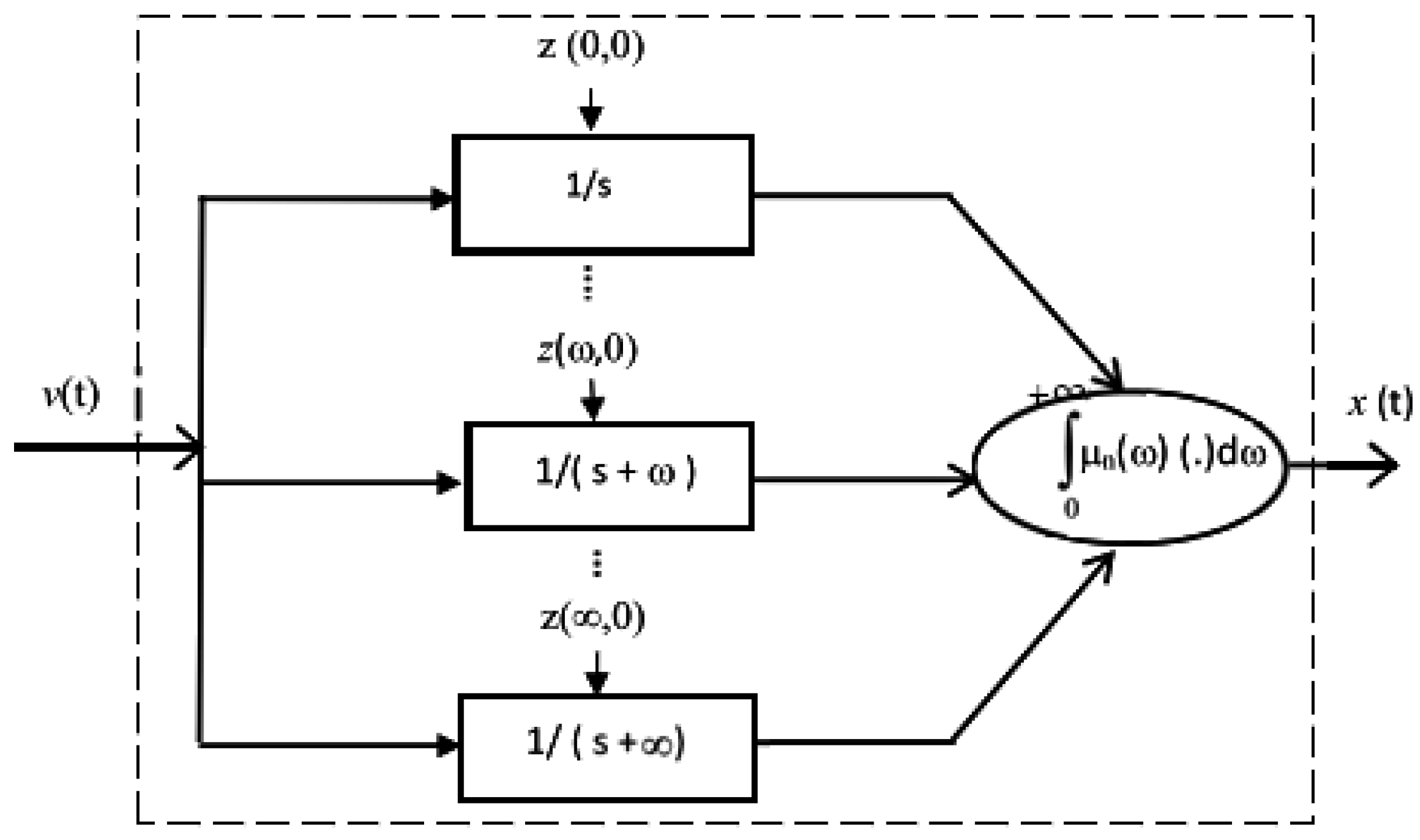
3.3. The Distributed Model of the Fractional Integrator

Based on the previous definition, it is obvious that fractional integration is a more complex operation than usual integer-order integration since it corresponds to the convolution of v ( t ) with the impulse response h n ( t ) . This convolution is numerically difficult to perform with the previous definition of the impulse response. In fact, we can use another expression of h n ( t ) derived from the inverse Laplace transform of 1 s n .
For 0 < n < 1 and using a Bromwich contour (chap.6 vol.1 in [22]), we obtain the following:
h n ( t ) = 0 μ n ( ω ) e ω t d ω     0 < n < 1 μ n ( ω ) = sin ( n π ) π ω n
which is equivalent to the following:
1 s n = 0 μ n ( ω ) 1 s + ω d ω       0 < n < 1
where 1 s + ω is one of the elementary modes of the fractional integrator.
More generally, the fractional integrator output x ( t ) , which is the response to an input v ( t ) , is the solution of the frequency-distributed integer-order model:
z ( ω , t ) t = ω z ( ω , t ) + v ( t )     ω 0 , x ( t ) = 0 μ n ( ω ) z ( ω , t ) d ω μ n ( ω ) = sin ( n π ) π ω n     0 < n < 1
Figure 3 displays the graphical representation of Equation (8) where z ( ω , t ) is the frequency-distributed state variable of the fractional integrator; on the contrary, x ( t ) is not a true state variable because it is the weighted integral of the distributed states. It is for this reason that x ( t ) is called a pseudo-state variable.

3.4. Transients of the Frequency-Distributed Integrator

Consider the Laplace transform of (8) as follows:
s Z ( ω , s ) z ( ω , 0 ) = ω Z ( ω , s ) + V ( s )       ω 0 , X ( s ) = 0 μ n ( ω ) Z ( ω , s ) d ω
where z ( ω , 0 ) is the initial value of z ( ω , t ) at t = 0 , which summarizes the past behavior of the fractional integrator.
This means that the following:
X ( s ) = 0 μ n ( ω ) z ( ω , 0 ) s + ω d ω + 0 μ n ( ω ) V ( s ) s + ω d ω
Using Equation (7), we can write the following in the time domain:
x ( t ) = x 0 ( t ) + I t n v ( t )
where
x 0 ( t ) = 0 μ n ( ω ) z ( ω , 0 ) e ω t d ω
The free response of the fractional integrator initialized by the distributed initial conditions is z ( ω , 0 ) ω 0 , ;it is also called the initialization function and I t n v ( t ) is the forced response of the fractional integrator caused by the input v ( t ) .
Usually, according to the Volterra Equation (2), the response of the fractional integrator to any input v ( t ) is expressed as x ( t ) = I t n v ( t ) + x ( 0 ) where x ( 0 ) is derived from the so-called initial condition of the Caputo derivative. Of course, this formulation is wrong since x ( 0 ) has to be replaced by x 0 ( t ) .

4. Initial Conditions of the Caputo Derivative

4.1. Introduction

We have demonstrated with the elementary counter-example in Section 2 that the integration technique based on the Caputo derivative is unable to provide the correct expression of the free response of an elementary initial value problem. Of course, we have pointed out the reason for this failure, i.e., x ( 0 ) does not represent the initial condition of the fractional integrator.
The question is, what is the origin of this error?
In order to understand why so many researchers have been misled by the so-called “physical initial condition” x ( 0 ) , we have to remember the definition of the Caputo derivative [1] for 0 < n < 1 :
D t n C x ( t ) = I t 1 n d x ( t ) d t

4.2. Initial Conditions

This derivative basically relies on a fractional integrator 1 s 1 n , so we have to take into account its internal state variables z C ( ω , t ) at t = 0 (notice that z C ( ω , t ) z ( ω , t ) ).
Thus, the distributed model of the Caputo derivative is as follows:
z C ( ω , t ) t = ω z C ( ω , t ) + d x ( t ) d t      ω 0 , D t n C x ( t ) = 0 μ 1 n ( ω ) z C ( ω , t ) d ω μ 1 n ( ω ) = sin ( 1 n ) π π ω ( 1 n ) a n d 0 < n < 1
with the initial condition z C ( ω , 0 ) ω .
Using Laplace transform, we can write the following:
Z C ( ω , s ) = z C ( ω , 0 ) s + ω + L d x ( t ) d t s + ω      ω 0 , w i t h L d x ( t ) d t = s X ( s ) x ( 0 )
Thus, ref. [23] the following is calculated:
L D t n C x ( t ) = s n X ( s ) x ( 0 ) s 1 n + 0 μ 1 n ( ω ) s + ω z C ( ω , 0 ) d ω
We notice that the two first terms of (16) correspond to the usual definition of the initial condition x ( 0 ) , but the third term characterizes the distributed initial condition of the integrator 1 s 1 n and, consequently, x ( 0 ) can no longer be considered the only initial condition of the Caputo derivative. In (Chapter 8 volume 1 in [23]), we prove that the same error occurs with the Riemann–Liouville derivative. So, the conclusion is that the integration of FDEs or FDSs based on the usual initial conditions of the Caputo derivative or of the Riemann–Liouville derivative leads to erroneous free responses. However, these two techniques are the necessary tools for the practical calculation of the fractional derivative. Moreover, forced responses obtained with these techniques are correct because they do not depend on initial conditions. The properties and applications of these derivatives are, for example, exhibited in the books by Podlubny [1] and Diethelm [2].

5. Counter-Example: The Infinite State Solution

5.1. Introduction

It has been proved previously that the initial condition of the FDE D n ( x ) = a x ( t ) is not x ( 0 ) , which has to be replaced by the free response x 0 ( t ) of the fractional integrator, the distributed initial condition of which is z ( ω , 0 ) ω 0 , . Consequently, the first objective is to correct the free response based on the Mittag–Leffler function. The second objective is to demonstrate that this free response can be expressed more simply and efficiently by the I.S. technique. Moreover, based on the frequency-discretized model of the fractional integrator, numerical computations demonstrate the validity of these theoretical results.

5.2. The Mittag–LefflerApproach

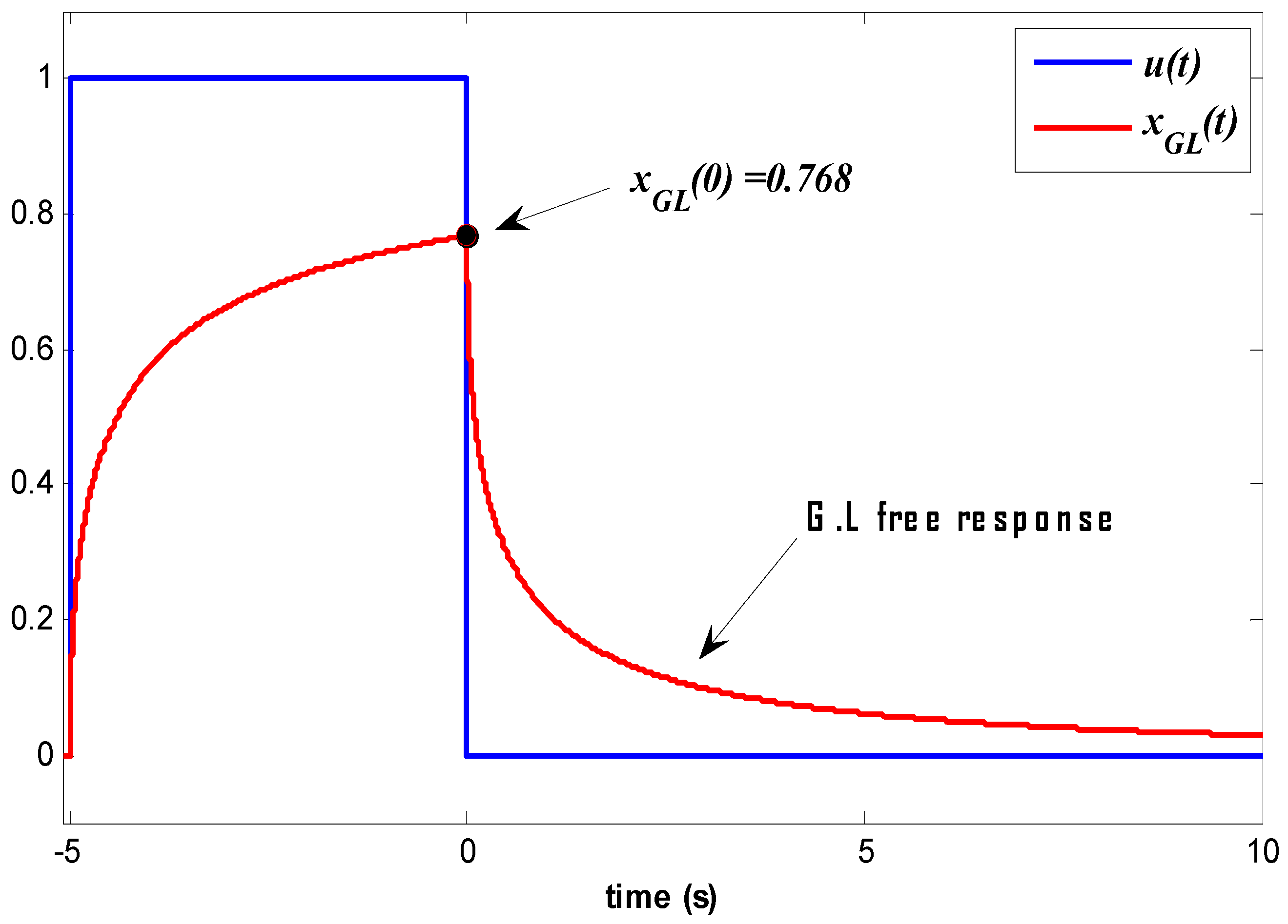
5.2.1. The Mittag–Leffler Free Response

Consider again the free response of (1), which is presented in Section 2. The elementary initial value problem was solved with the Volterra relation. However, we prove in Section 3 that the initial condition of 1 s n is x 0 ( t ) (also referred to [36]). So, replacing x ( 0 ) with x 0 ( t ) , we can obtain the following:
x M L ( t ) = I t n D t n C ( x M L ) = I t n 0 a x M L ( t ) + x 0 ( t )
Using the Laplace transform, we can write the following:
X M L ( s ) = 1 s n a X M L ( s ) + X 0 ( s ) ,   so   X M L ( s ) = s n X 0 ( s ) s n a = s s n 1 s n a X 0 ( s ) .
Using definition (3) again, we obtain the following:
x M L ( t ) = L 1 s L E n , 1 ( a t n ) X 0 ( s )     = d d t E n , 1 ( a t n ) x 0 ( t ) = E n , 1 ( a t n ) d d t x 0 ( t )
Remark 1.
If x 0 ( t ) = x ( 0 ) = c t e , we can write x 0 ( t ) = x ( 0 ) H ( t ) and d d t x 0 ( t ) = x ( 0 ) δ ( t ) . So, x M L ( t ) = E n , 1 ( a t n ) x ( 0 ) δ ( t ) = E n , 1 ( a t n ) x ( 0 ) , which is the usual Caputo solution.
The previous solution (18) exhibits a difficult problem, i.e., the convolution of the Mittag–Leffler function with the free response derivative of the fractional integrator. In fact, it is possible to re-interpret it as a more classical problem. Using the definition of x 0 ( t ) , i.e., x 0 ( t ) = 0 μ n ( ω ) z ( ω , 0 ) e ω t d ω , we can write the following:
x M L ( t ) = d d t E n , 1 ( a t n ) x 0 ( t ) = 0 μ n ( ω ) d d t z ( ω , 0 ) E n , 1 ( a t n ) e ω t d ω
Let us define v ( ω , t ) and η ( ω , t ) as follows:
v ( ω , t ) = z ( ω , 0 ) E n , 1 ( a t n ) e ω t η ( ω , t ) = d d t v ( ω , t )
First, we note that e ω t is the impulse response of the elementary first-order system 1 s + ω . So, we can consider that v ( ω , t ) is the forced response of the elementary system to the input z ( ω , 0 ) E n , 1 ( a t n ) and we can obtain the following:
x M L ( t ) = 0 μ n ( ω ) η ( ω , t ) d ω

5.2.2. Principle of the Numerical Computation of the Mittag–Lefler Free Response

Using the discretized approximation of the fractional integrator (Appendix B), we can compute v j ( t ) and η j ( t ) with the distributed differential system as follows:
η j ( t ) = d v j ( t ) d t = ω j v j ( t ) + z j ( 0 ) E n , 1 ( a t n )       j = 0 t o J x M L ( t ) = j = 0 J c j η j ( t )
Finally, time discretization with the sampling period T e provides the following:
v j , k = α j v j , k 1 + β j z j ( 0 ) E n , 1 a t k 1 n η j , k = v j , k v j , k 1 T e x M L ( k ) = j = 0 J c j η j , k
The previous convolution technique (19) requires the knowledge of the initial conditions of 1 s n , i.e., z ( ω , 0 ) ω 0 , , which depends on the past history of the system D n ( x ) = a x ( t ) + u ( t ) on t T , 0 , which includes the history of the frequency-distributed system as follows:
z ( ω , t ) t = ω z ( ω , t ) + a x ( t ) + u ( t ) ω       0 , x ( t ) = 0 μ n ( ω ) z ( ω , t ) d ω μ n ( ω ) = sin ( n π ) π ω n 0 < n < 1
or practically with the distributed frequency approximation:
d z j ( t ) d t = ω j z j ( t ) + a x ( t ) + u ( t )       j = 0 t o J x ( t ) = j = 0 J c j z j ( t )
knowing that the only available information is x G L ( t ) t T , 0 and the practical objective is to estimate z j ( 0 )    j = 0    t o J .
The classical solution to estimate the system state is to use a Luenberger observer [37], the model of which is the following:
D n ( x ) = a x ( t ) + u ( t ) + G x G L ( t ) x ( t )
where x ( t ) is the estimate of x G L ( t ) and G is the observer gain.
So, using the distributed discretized model, we obtain the following z j ( 0 ) estimates:
d z j ( t ) d t = ω j z j ( t ) + a x ( t ) + u ( t ) + G ( x G L ( t ) x ( t ) )        j = 0 t o J x ( t ) = j = 0 J c j z j ( t )
where z j ( t ) is the estimate of the integrator frequency-distributed state z j ( t ) .
In order to quantify the observer performance, we have to know the reference values of z j ( t ) . They are provided by the simulation of the model (25) in parallel with the G.L. technique. Because the two simulations x G L ( t ) and x I S ( t ) are very close to each other, we computed the Mean Absolute Error (MAE) criterion for t T , 0 with K = T T e :
C I S = k = 0 K x G L ( k ) x I S ( k ) K + 1

5.2.3. Numerical Example of the Computation of the Mittag–Leffler Free Response

First, we simulate the system (25) on t T , 0 with J = 50 , ω min = 10 6 , ω max = 10 3 .
Thus, we obtain C I S = 1.16 10 5 ; x ( 0 ) = 0.768 . The corresponding distributed states z j ( 0 ) at t = 0 and for j = 0 to J are displayed (blue curve) in Figure 4a.
Then, we compute the observer (27) with G = 50 . The estimated values z j ( 0 ) are plotted (green curve)in Figure 4a. As can be seen, the two graphs are very close, with only a slight difference at very low frequencies.
Remark 2.
Since the system (25) is at rest at t = T , the observer also starts to rest at t = T . More generally, the system is not at rest when the observer starts, so there is an unknown initial condition of the system that acts as a disturbance to the observer. In order to appreciate the influence of this unknown initial state, we performed another experiment where the observer starts at t = T + Δ T , with  Δ T = 0.5 s .
This second estimated distribution is also plotted in Figure 4b. Thus, we can see that the disturbance only modifies the estimates at very low frequencies.
Finally, we compute the free response x M L ( t ) with Equations (22) and (23) using the previous estimates z j ( 0 ) . Since the graphs of x G L ( t ) and x M L ( t ) are also very close to each other, we can compute another MAE criterion for t 0 , 2 T with K * = 2 T T e :
C M L = k = 0 K * x G L ( k ) x M L ( k ) K * + 1
Thus, we obtain C M L = 8.41 × 10 5 , which means that the theoretical Equation (21) is verified.
As we also performed another estimate of z j ( 0 ) with the disturbed observer, we again computed the free response x M L ( t ) . The graphs of x G L ( t ) and x M L ( t ) are also very close ( C M L = 1.6 × 10 4 ) since the effect of poorer low frequency estimates of z j ( 0 ) appears mainly for large values of t .
Thus, we can conclude that the free response of D n ( x ) = a x ( t ) depends on the initial state z ( ω , 0 ) ω 0 , of the fractional integrator rather than on x ( 0 ) , as erroneously stated by the usual Caputo approach.

5.3. The Infinite State Approach

5.3.1. Introduction

The previous methodology is relatively complex since it is related to the convolution of the Mittag–Leffler function with the free response of the associated fractional integrator. Moreover, it is well known that the computation of the M.L. function is very sensitive to large values of t . Nevertheless, this technique could be generalized as follows:
D n ( X ¯ ) = A X ¯ ( t ) + u ( t ) dim X ¯ = N
using the matrix M.L. function [4]. Consequently, the computation of the free response of D n ( X ¯ ) = A X ¯ ( t ) is a hard task. However, the main interest of this technique has been to prove that the correct computation of transient dynamics is no longer an unsolved problem, replacing the erroneous initial condition x ( 0 ) by x 0 ( t ) (or X ¯ ( 0 ) by X ¯ 0 ( t ) ).
In fact, since we introduced the distributed system states z ( ω , t ) ω 0 , , there was a direct solution to the computation of transient dynamics.

5.3.2. Direct Numerical Solution

Consider the initial value problem D n ( x ( t ) ) = a x ( t ) with the initial condition z ( ω , 0 )    ω 0 , or practically z j ( 0 ) j = 0 t o J . Using the distributed model of the fractional integrator with the finite-dimensional approximation (Appendix B), the following is calculated:
d z j ( t ) d t = ω j z j ( t ) + a x ( t )       j = 0 t o J x ( t ) = j = 0 J c j z j ( t )
Based on the initial condition z j ( 0 ) j = 0 t o J , we can compute z j ( t ) j = 0 t o J and x ( t ) .
The simulation of this system composed of J + 1 ODEs is an obvious problem, and the solution is the weighted sum of the elementary solutions z j ( t ) . It requires knowledge of the initial conditions z j ( 0 ) which is given by the previous observer. The free responses x G L ( t ) and x I S ( t ) are again very close, so we can judge the accuracy of this technique with the MAE criterion C I S .
Thus, with J = 50 , ω min = 10 6 , ω max = 10 3 , T e = 10 3 s , we obtain C I S = 8.43 × 10 5 .
As C I S and C M L are very close values again, this means that the two techniques provide identical free responses.

5.3.3. The Matrix Exponential Solution

The previous differential system (31) can be expressed in vector form using Equations (A12) and (A13) in Appendix B.
Let Z ¯ T ( t ) = z 0 ( t ) z j ( t ) z J ( t ) and Z ¯ T ( 0 ) = z 0 ( 0 ) z j ( 0 ) z J ( 0 ) .
Then, system (31) becomes the following:
d Z ¯ ( t ) d t = A s y s t Z ¯ ( t ) x ( t ) = C ¯ I Z ¯ ( t )
with initial condition Z ¯ ( 0 ) and A s y s t = A I + a B ¯ I C ¯ I .
Since (32) is an integer-order differential system, with dim ( Z ¯ ) = J + 1 , its solution can be expressed with the matrix exponential e A s y s t t :
Z ¯ ( t ) = e A s y s t t Z ¯ ( 0 ) x ( t ) = C ¯ I Z ¯ ( t )
It is important to note that this technique permits the computation of Z ¯ T ( t ) and x ( t ) without the necessary computation of the intermediary solutions given by the simulation technique. Fundamentally, this means that the I.S. technique, which is based on the transformation of the original fractional-order system into a set of J + 1 integer-order differential systems, verifies the semi-group property [38], contrary to the matrix Mittag–Leffler function [4].
Since the system (32) is strictly equivalent to (31), the two solutions are identical. Of course, this matrix exponential solution also applies to the following general representation:
D n ¯ ( X ¯ ) = A X ¯ ( t ) + u ( t )      dim X ¯ = N
where n ¯ can be composed of N different fractional orders. Refer to (Chapter 9 volumw 1 in [22]) for more information on the distributed matrix exponential.

6. Why Is the Usual Caputo Solution Unrealistic?

6.1. Introduction

In Section 4, we analyzed the initial conditions of the Caputo derivative, which refer to x ( 0 ) and to the distributed state at t = 0 of the integrator 1 s 1 n , i.e., z C ( ω , 0 ) ω 0 , . So the only remaining initial condition can be x ( 0 ) if z C ( ω , 0 ) = 0 ω 0 , , i.e., if the system has been at rest ( d x ( t ) d t = 0 ) fora long time in the past. This is a restrictive condition that many researchers only consider as a mathematical and acceptable assumption, but is it a realistic condition?
Based on numerical simulations, we prove in this last section that this condition is not only restrictive but completely unrealistic.

6.2. Necessary Condition for Rest Based on the History Interval

In Section 2, we consider an initial condition at t = 0 caused by the action of a step input u ( t ) = U H ( t T ) on the interval T , 0 . We also prove that x ( 0 ) results of the weighted sum of the distributed state variables is z ( ω , t ) at t = 0 , or it practically is so for the discretized variables z j ( t ) at t = 0 since the following is calculated:
x ( 0 ) = 0 μ n ( ω ) z ( ω , 0 ) d ω or   x ( 0 ) = j = 0 J c j z j ( 0 ) .
So, what is the realistic condition on T in order to consider that the system is completely at rest at t = 0 ?
Consider the elementary system D n ( x ( t ) ) = a x ( t ) + u ( t ) and a step input u ( t ) = U H ( t ) applied at t = 0 . Using the Laplace transform, we can write the following:
X ( s ) = 1 s n a U s
with a = 1    U = 1 , we obtain x ( ) = lim s 0 s U s ( s n a ) = 1 .
Notice that x ( ) corresponds to x ( 0 ) for the counter-example.
So, the question is how can we chose T to obtain x ( T ) U ?
Since Z ( ω , s ) = s n s + ω ( s n + a ) U s ,we obtain the following:
Z ( ω , s ) = s n s s + ω ( s n + a ) U
As z ( ω , ) = lim s 0 s Z ( ω , s ) we obtain z ω , = 0 ω 0 and z ( 0 , ) = lim s 0 s Z ( 0 , s ) = .
Notice that x ( ) has a finite value whereas z ( 0 , ) , which is the modal component of x ( t ) at ω = 0 , has an infinite value. The elementary system is at rest (i.e., it has reached x ( ) ) if all its state variables are equal to zero, except for ω = 0 ). Practically, using the frequency approximation ( x ( t ) = j = 0 J c j z j ( t ) ), the system is at rest if all the state variables ( j = 1 t o J ) are equal to zero, except for j = 0 . So x ( ) = c 0 z 0 ( ) is the discrete approximation of x ( ) = lim ω 0 0 μ n ( ω ) z ( ω , ) d ω .
In order to quantify the influence of T on system rest, we plot, in Figure 5 and Figure 6, the graphs of x ( t ) and of the distributed state variables z j ( T ) for increasing values of T .
For T = 1 s , we notice that the higher frequency modes have approximately the same amplitude as the lower frequency ones. Of course, for T = 1 s , x ( T ) is far from reaching x ( ) = 1 . On the contrary, as T increases, since the higher frequency modes gradually move toward zero, the lower frequency modes have a more important influence on the value of x ( T ) . However, even for T = 1 000 s , the modes close to ω = 0 are not exactly equal to zero (except for j = 0 ). This means that it would be necessary to use T > > 1000 s to obtain x ( T ) U . Obviously, this is not a realistic condition.

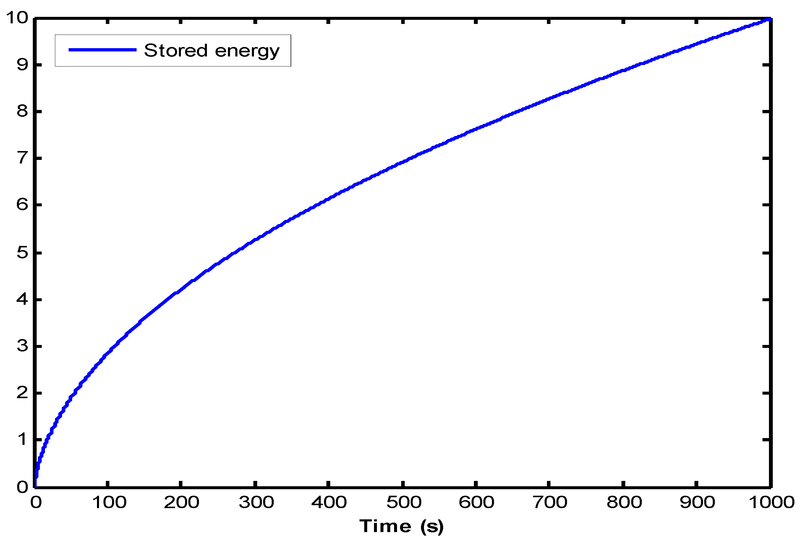
6.3. Stored Energy in the Fractional Integrator

The previous simulations have demonstrated that the necessary condition T to achieve system rest is not a realistic condition for a fractional-order system, but nevertheless, is it physically realistic? To give an answer to this question, we consider the energy stored in the system, i.e., in the fractional integrator.
In the integer-order case, i.e., n = 1 , the integer-order integrator 1 s is characterized by only one state variable x ( t ) (i.e., only one mode at ω = 0 ), and its energy is proportional to x ( t ) 2 , i.e., the stored energy is as follows:
E 1 ( T ) = 1 2 x ( T ) 2
So, T with U = 1 , x ( T ) 1 and E 1 ( ) = 1 2 , which is a finite value.
Obviously, the energy stored in the integrator is never considered in the integer-order case. The situation is completely different in the fractional-order case.
We also note that x ( t ) = 0 μ n ( ω ) z ( ω , t ) d ω . It has been proved (chap.7 vol.2 in [22]) that the energy stored at instant t in the fractional integrator is the weighted sum of the elementary energies z ( ω , t ) 2 in the different modes ω , as follows:
E n ( T ) = 1 2 0 μ n ( ω ) z ( ω , T ) 2 d ω
or approximately
E n ( T ) = 1 2 j = 0 J c j z j ( T ) 2
Within the previous numerical simulations, we calculated E n ( T ) for increasing values of T . The corresponding graph is plotted in Figure 7. Contrary to the integer-order case, the energy stored in the system (i.e., in the associated fractional integrator) is not constant since it increases with T .
In (chap.7 vol.2 in [22]), using the diffusive representation (which is equivalent to I.S. representation (chap.7 vol.1 in [22]), we prove theoretically that the energy stored in the system for a step input is infinite when T is very large, i.e., E n ( T ) a s T . Obviously, this is not an intuitive result, contrary to the integer-order case. This is an unknown feature of the fractional integrator, which is only revealed by an I.S. approach. This result was also proved mathematically with a different approach in [39]; previous simulations have illustrated this fundamental result.
Therefore, we can conclude that the so-called “physical initial condition” of the Caputo derivative is not only unrealistic but physically unrealistic because it would correspond to infinite stored energy.

7. Conclusions

As stressed in the introduction, it has been proved that the so-called physical initial condition of the Caputo derivative is unable to solve fractional-order transient dynamics. The origin of this failure has been analyzed, and a realistic and satisfactory solution based on the I.S. representation has been proposed. Moreover, numerical simulations have demonstrated that the usual Caputo approach is based on an initial condition that is not only unrealistic but completely without physical meaning.
The complexity of the I.S. approach is the necessary price to pay for the correct modeling of fractional-order transients. This technique is also the complement of the usual fractional approach, as illustrated by the treatment of the convolution between the M.L. function and the free response of the fractional integrator. Although the example presented in the paper is deliberately simple for a didactic purpose, the object of the I.S. technique is general, and it applies either to more complex problems like fractional optimal control or to nonlinear systems and fractional chaotic systems in particular [23].
The criticism of the usual Caputo derivative approach is not a denial of the fractional calculus theory. On the contrary, the objective of the paper is to provide a faultless foundation for fractional initial value problems and transient dynamics in order to stimulate new theoretical and applied research works.

Author Contributions

Methodology, J.-C.T. and N.M.; writing—original draft preparation, J.-C.T. and N.M.; writing—review and editing, J.-C.T. and N.M. All authors have read and agreed to the published version of the manuscript.

Funding

This research received no external funding.

Data Availability Statement

Data are contained within the article.

Conflicts of Interest

The authors declare no conflicts of interest.

Appendix A. The Grünwald–Letnikov Integrator

The Nth integer-order Euler derivative of f ( t ) is defined as follows:
D N f ( t ) t = k h = lim T e 0 1 q 1 N T e N f k ,
where f k = f ( k ) , f ( k 1 ) , f ( k i ) and q 1 is the delay operator.
The generalization to the fractional case n > 0 provides the Grünwald–Letnikov derivative [1]:
D n G L f ( t ) t = k h = lim T e 0 1 q 1 n T e n f k
Since L q 1 = e T e s we obtain the following:
L D n G L f ( t ) = lim T e 0 1 e T s s n T e n L f ( t ) = s n F ( s ) ,
Notice that
1 q 1 n T e n = 1 T e n 1 + i = 0 α i , G L q i ,
with α i , G L = ( 1 ) i n 1 n 1 2 n 2 3 n ( i + 1 ) i ,
so   D n G L f ( t ) t = k h = 1 + i = 0 α i , G L q i T e n f k
which is the Moving Average formulation of the Grünwald–Letnikov derivative.
Reciprocally, we can define the Grünwald–Letnikov integral operator as follows:
I n G L q 1 = T e n q 1 1 + i = 0 α i , G L q i
which is the Auto-Regressive formulation of the Grünwald–Letnikov integrator.
Notice that L I n G L f ( t ) = lim T e 0 T e n e T e s 1 e T e s n L f ( t ) = 1 s n F ( s ) , which means that the Grünwald–Letnikov integrator is the time discretization of the Riemann–Liouville integrator.
Then, the elementary FDE initial value problem can be considered:
D t n x ( t ) = f x ( t ) , u ( t )        0 < n < 1
Using the Grünwald–Letnikov integrator, we can express x ( k ) as follows:
x ( k + 1 ) = I n G L f x k , u k + g x i n i t
where x i n i t = x ( 0 ) , x ( 1 ) , , x ( i ) , , x ( ) .
This means that the initial condition of the system (A4) is composed of all the past values of x ( i ) since k = .
Practically, this technique can be used for the numerical simulation of any FDE problem with excellent accuracy. The interested reader can refer to (Chapter 3 volume 1 in [22]), where different applications of the G.L. integral and the short memory principle [1] are analyzed.

Appendix B. Finite-Dimensional Approximation of the Fractional Integrator

The finite-dimensional approximation is a fundamental topic for the practical use of I.S. representation; moreover, it has to take into account singularities of the weighting function μ n ( ω ) and of the frequency response.
This approach is based on the following frequency response:
1 s n s = j ω = ρ ( ω ) ; θ ( ω ) ρ ( ω ) = 1 ω n ; θ ( ω ) = n π 2
Since ρ ( 0 ) , there is a singularity for ω = 0 .

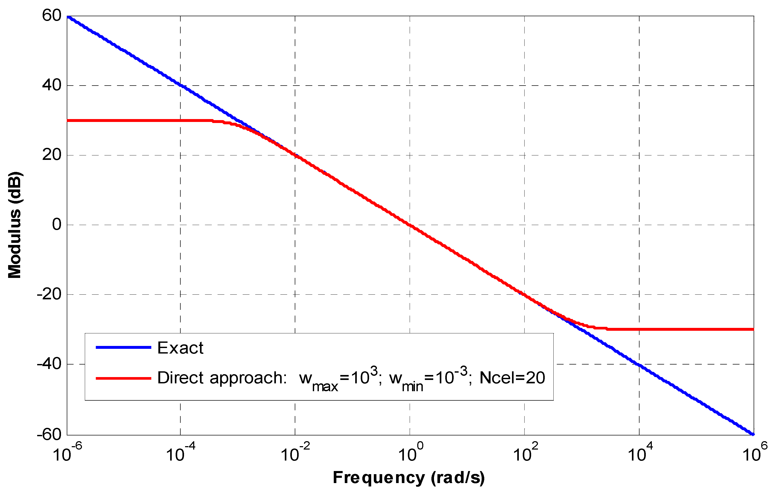
Appendix B.1. Direct Approach

Using the reciprocal of Oustaloup’s differentiator [40] in the frequency band ω min ; ω max , we can obtain an approximation of the fractional integrator:
1 s n G n 1 + s ω max 1 + s ω min n
corresponding to the graph in Figure A1.
Figure A1. Frequency response of the direct approximation of 1 s 0.5 .
Fractalfract 09 00252 g0a1
Notice that this graph tends to a finite value for ω = 0 , in contradiction with the true integrator behavior. Moreover, because the gain of the direct approach is not infinite at ω = 0 , this approximation is not adapted to the usual FDE simulation and it modifies the fixed points of fractional chaotic systems, leading to fake fractional attractors [41].

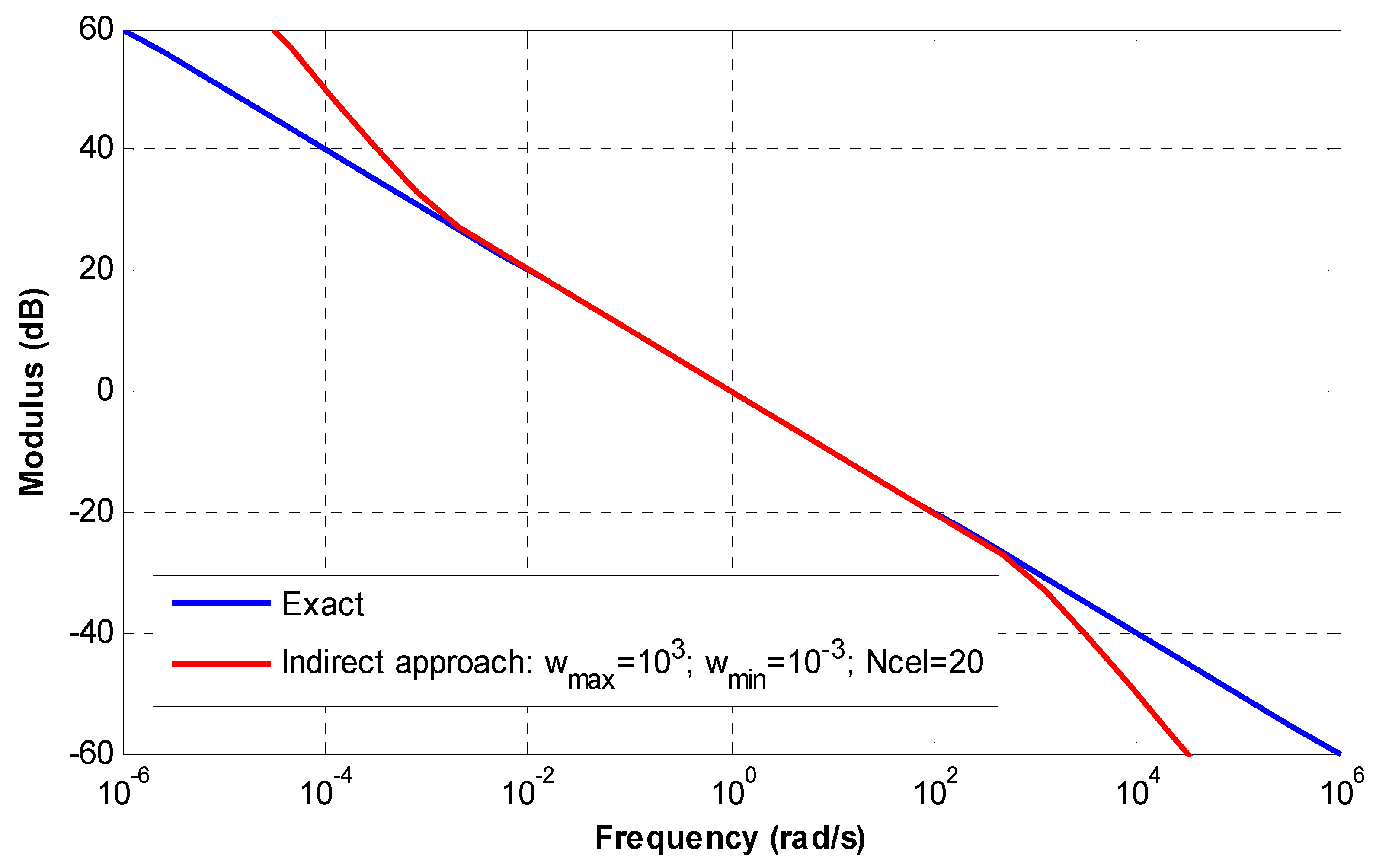
Appendix B.2. Indirect Approach

In order to solve the previous difficulty, an integer integrator 1 s has been associated with a fractional differentiator s 1 n such that the following is calculated:
1 s n G n s 1 + s ω min 1 + s ω max 1 n
corresponding to the graph in Figure A2.
Figure A2. Frequency response of the indirect approximation of 1 s 0.5 .
Fractalfract 09 00252 g0a2

Appendix B.3. Frequency-Discretized Approximation

This approximation was used for all our numerical simulations. Practically, this model corresponds to the frequency-discretized approximation with ( J + 1 ) modes varying from ω 0 = 0 to ω J in the frequency band ω min ; ω max :
d z j ( t ) d t = ω j z j ( t ) + v ( t )       j = 0 t o J x ( t ) = j = 0 J c j z j ( t )
Refer to [22] for details on the computation of ω j and c j with Oustaloup’s method.
The time discretization of (A9) with sampling time T e ( t = k T e ) leads to the following recursive algorithm:
z j , k = α j z j , k 1 + β j v k 1 x k = j = 0 J c j z j , k
In order to avoid numerical instability due to too-small values of T e , α j and β j are computed with the Z transform technique [22]:
α j = e ω j T e      β j = 1 α j ω j
The recursive algorithm (A10) is an efficient technique with which to perform the convolution equation x ( t ) = h n ( t ) v ( t ) .
The model (A10) can also be used with matrix formulation. The following are defined:
Z ¯ T ( t ) = z 0 ( t ) z j ( t ) z J ( t )       dim Z ¯ = J + 1 A I = ω 0 0 ω j 0 ω J B I T ¯ = 1 1 1           C I ¯ = c 0 c j c J
Then, the previous model (A10) is transformed into the following:
d d t Z ¯ ( t ) = A I Z ¯ ( t ) + B ¯ I v ( t )       x ( t ) = C I ¯ Z ¯ ( t )

References

  1. Podlubny, I. Fractional Differential Equations; Academic Press: San Diego, CA, USA, 1999. [Google Scholar]
  2. Diethelm, K. The Analysis of Fractional Differential Equations; Lecture Notes in Mathematics; Springer: Berlin/Heidelberg, Germany, 2010. [Google Scholar]
  3. Podlubny, I. Geometric and physical interpretation of fractional integration and fractional differentiation. Fract. Calc. Appl. Anal. 2002, 5, 367–386. [Google Scholar]
  4. Monje, C.A.; Chen, Y.Q.; Vinagre, B.M.; Xue, D.; Feliu, V. Fractional Order Systems and Control; Springer: London, UK, 2010. [Google Scholar]
  5. Fukunaga, M.; Shimizu, N. Role of prehistories in the initial value problems of fractional viscoelastic equations. Nonlinear Dyn. 2004, 38, 207–220. [Google Scholar] [CrossRef]
  6. Hartley, T.T.; Lorenzo, C.F. The error incurred in using the Caputo derivative Laplace transform. In Proceedings of the ASME IDET-CIE Conferences, San Diego, CA, USA, 30 August–2 September 2009. [Google Scholar]
  7. Sabatier, J.; Merveillaut, M.; Malti, R.; Oustaloup, A. How to impose physically coherent initial conditions to a fractional system? Commun. Nonlinear Sci. Numer. Simul. 2010, 15, 1318–1326. [Google Scholar] [CrossRef]
  8. Du, M.; Wang, Z. Correcting the initialization of models with fractional derivatives via history dependent conditions. Acta Mech. Sin. 2015, 37, 320–325. [Google Scholar] [CrossRef]
  9. Du, B.; Wei, Y.; Liang, S.; Wang, Y. Estimation of exact initial states of fractional order systems. Nonlinear Dyn. 2016, 86, 2061–2070. [Google Scholar] [CrossRef]
  10. Zhao, Y.; Wei, Y.; Chen, Y.; Wang, Y. A new look at the fractional initial value problem: The aberration phenomenon. ASME J. Comput. Nonlinear Dyn. 2018, 13, 121004. [Google Scholar] [CrossRef]
  11. Balin, A.M.; Balint, S. Mathematical description of the groundwater flow and that of the impurity spread, which use temporal Caputo or Riemann–Liouville fractional partial derivatives, is non-objective. Fractal Fract. 2020, 4, 36. [Google Scholar] [CrossRef]
  12. Khalil, A.; Yousef, M.S. A new definition of fractional derivative. J. Comput. Appl. Math. 2014, 264, 65–70. [Google Scholar] [CrossRef]
  13. Caputo, M.; Fabrizio, M. A new definition of fractional derivative without singular kernel. Prog. Fract. Differ. Appl. 2015, 2, 73–85. [Google Scholar]
  14. Atanackovic, T.M.; Pilipovic, S.; Zorica, D. Properties of the Caputo-Fabrizio fractional derivative and its distributional setting. Fract. Calc. Appl. Anal. 2018, 21, 29–44. [Google Scholar] [CrossRef]
  15. Martinez, F.; Mohammed, P.O.; Valdes, J.N. Non-conformable fractional Laplace transform. Kragujev. J. Math. 2022, 46, 341–354. [Google Scholar] [CrossRef]
  16. Ortigueira, M.D.; Machado, J.T. A critical analysis of the Caputo-Fabrizio operator. Commun. Nonlinear Sci. Numer. Simulat. 2018, 59, 608–611. [Google Scholar] [CrossRef]
  17. Tarasov, V.E. No nonlocality, no fractional derivative. Commun. Nonlinear Sci. Numer. Simulat. 2018, 62, 157–163. [Google Scholar] [CrossRef]
  18. Hartley, T.T.; Lorenzo, C.F. The initialization response of linear fractional order system with constant History function. In Proceedings of the 2009 ASME/IDETC, San Diego, CA, USA, 30 August–2 September 2009. [Google Scholar]
  19. Hartley, T.T.; Lorenzo, C.F. The initialization response of linear fractional order system with ramp History function. In Proceedings of the 2009 ASME/IDETC, San Diego, CA, USA, 30 August–2 September 2009. [Google Scholar]
  20. Maamri, T.J.C.N.; Oustaloup, A. The infinite state approach: Origin and necessity. Comput. Math. Appl. 2013, 66, 892–907. [Google Scholar]
  21. Hartley, T.T.; Lorenzo, C.F.; Trigeassou, J.C.; Maamri, N. Equivalence of history function based and infinite dimensional state initializations for fractional order operators. ASME J. Comput. Nonlinear Dyn. 2013, 8, 041014. [Google Scholar] [CrossRef]
  22. Trigeassou, J.C.; Maamri, N. Analysis, Modeling and Stability of Fractional Order Differential Systems 1: The Infinite State Approach; John Wiley and Sons: Hoboken, NJ, USA, 2019; Volume 1–2. [Google Scholar]
  23. Trigeassou, J.C.; Maamri, N. The Infinite State representation of fractional order differential systems: A survey, parts I and II. IFAC-PapersOnLine 2024, 58, 265–275. [Google Scholar] [CrossRef]
  24. Wang, B.; Ding, J.; Wu, F.; Zhu, D. Robust finite time control of fractional order nonlinear systems via frequency distributed model. Nonlinear Dyn. 2016, 85, 2133–2142. [Google Scholar] [CrossRef]
  25. Yuan, J.; Zhang, Y.; Liu, J.; Shi, B. Equivalence of initialized fractional integrals and the diffusive model. ASME J. Comput. Nonlinear Dyn. 2018, 13, 034501. [Google Scholar] [CrossRef]
  26. Yuan, J.; Shi, B.; Ji, W. Adaptive sliding mode control of a novel class of fractional chaotic systems. Adv. Math. Phys. 2013, 2013, 576709. [Google Scholar] [CrossRef]
  27. Wang, B.; Yin, L.; Wang, S.; Mia, S.; Du, T. Finite time control for fractional order nonlinear hydroturbine governing system via frequency distributed model. Hindawi Math. Phys. 2016, 2016, 7345325. [Google Scholar] [CrossRef]
  28. Montseny, G. Diffusive representation of pseudo differential time operators. ESAIM Proc. 1998, 5, 159–175. [Google Scholar] [CrossRef]
  29. Heleschewitz, D.; Matignon, D. Diffusive realizations of fractional integro-differential operators: Structural analysis under approximation. In Proceedings of the IFAC, System, Structure and Control, Nantes, France, 8–10 July 1998; Volume 31, pp. 227–232. [Google Scholar]
  30. Diethelm, K. Fast solution methods for fractional differential equations in the modeling of viscoelastic materials. In Proceedings of the 9th ICSC Conference, Caen, France, 24–26 November 2021. [Google Scholar]
  31. Diethelm, K. A new diffusive representation for fractional derivatives, part I: Construction, implementation and numerical examples. In Fractional Differential Equations; Springer: Berlin/Heidelberg, Germany, 2022. [Google Scholar]
  32. Diethelm, K. A new diffusive representation for fractional derivatives, part II: Convergence analysis of the numerical scheme. Mathematics 2022, 10, 1245. [Google Scholar] [CrossRef]
  33. Hinze, M.; Schmidt, A.; Leine, R.I. Lyapunov stability of a fractionally damped oscillator with linear (anti-)damping. Int. J. Nonlinear Sci. Numer. Simul. 2020, 21, 425–442. [Google Scholar] [CrossRef]
  34. Hinze, M.; Schmidt, A.; Leine, R.I. Numerical solution of fractional ordinary differential equations using the reformulated infinite state representation. Fract. Calc. Appl. Anal. 2019, 22, 1321–1350. [Google Scholar] [CrossRef]
  35. Arumugam, V.; Ferrante, A.; Ntogramatzidis, L.; Padula, F. A geometric framework for distributed frequency models. Commun. Nonlinear Sci. Numer. Simul. 2024, 136, 108088. [Google Scholar] [CrossRef]
  36. Maamri, N.; Trigeassou, J.C. A plea for the integration of fractional differential systems: The initial value problem. Fractal Fract. 2022, 6, 550. [Google Scholar] [CrossRef]
  37. Maamri, N.; Tari, M.; Trigeassou, J.C. Improved initialization of fractional order systems. IFAC-PapersOnLine 2017, 50, 8567–8573. [Google Scholar] [CrossRef]
  38. Curtain, R.F.; Zwart, H.J. An Introduction to Infinite Dimensional Linear Systems Theory; Springer: New York, NY, USA, 1995. [Google Scholar]
  39. Hartley, T.T.; Trigeassou, J.C.; Lorenzo, C.F.; Maamri, N. Initialization energy in fractional order systems. In Proceedings of the ASME Conference IDETC/CIE, Boston, MA, USA, 2–5 August 2015. [Google Scholar]
  40. Oustaloup, A.; Levron, F.; Mathieu, B.; Nanot, F.M. Frequency-band complex noninteger differentiator: Characterization and synthesis. Trans. Circuits Syst. I Fundam. Theory Appl. 2000, 47, 25–39. [Google Scholar] [CrossRef]
  41. Tavazoei, M.S.; Haeri, M. Limitations of frequency domain approximation for detecting chaos in fractional order systems. Nonlinear Anal. 2008, 69, 1299–1320. [Google Scholar] [CrossRef]
Figure 1. A realistic initial value problem n = 0.5 .
Fractalfract 09 00252 g001
Figure 2. The reference and the Caputo free responses n = 0.5.
Fractalfract 09 00252 g002
Figure 3. Distributed representation of the fractional integrator.
Fractalfract 09 00252 g003
Figure 4. (a) Frequency-distributed states with G = 50 a n d Δ T = 0 s   n = 0.5 ; (b) frequency-distributed states with G = 50 a n d Δ T = 0.5 s   n = 0.5 .
Fractalfract 09 00252 g004
Figure 5. Step response of the elementary FDE: U = 1    n = 0.5 .
Fractalfract 09 00252 g005
Figure 6. Evolution of the frequency-distributed states with T .
Fractalfract 09 00252 g006
Figure 7. Stored energy in the elementary FDE U = 1    n = 0.5 .
Fractalfract 09 00252 g007
Disclaimer/Publisher’s Note: The statements, opinions and data contained in all publications are solely those of the individual author(s) and contributor(s) and not of MDPI and/or the editor(s). MDPI and/or the editor(s) disclaim responsibility for any injury to people or property resulting from any ideas, methods, instructions or products referred to in the content.

