A Simple Fractional Model with Unusual Dynamics in the Derivative Order

Abstract

Fractional variable order systems with unusual dynamics in the order are a little-studied topic. In this study, we present three examples of very simple fractional systems with unusual dynamics in the derivative order. These cases involve different approaches to define the variable-order dynamics: (1) an integer-order differential equation that includes the state variable, (2) a differential equation that incorporates the state variable and features both integer- and fractional-order derivatives, and (3) fractional variable-order differential equations nested in the derivative orders. We prove a result that shows how the extended recursion of the last case is generalized. These examples illustrate the richness that simple dynamical systems can reveal through the order of their derivatives.

1. Introduction

In the last few years, several types of non-integer calculus constructed with new derivatives and integrals have been presented [1,2]. These have generated many applications in several fields such as physics, engineering, finance, biology, medicine, chemistry and other disciplines [3,4,5,6]. They have also generated theoretical developments related to these new calculations in areas such as differential equations, inequalities, and dynamical systems, among others [7,8]. Some of these operators have been produced using modifications of previously formed operators. Among these operators are fractional operators of distributed order, fractional operators of variable order, and fractional operators that depend on a function [9,10,11,12,13]. This adds new characteristics to the new operators, therefore generating new possibilities for applications and theoretical developments.

When some phenomenon or system presents non-local properties or persistent memory that may vary with respect to time, space, or other variables, it is necessary to resort to variable-order (VO) operators.

Several proposals have been made in recent years, starting with the Scarpi derivative based on the Laplace transform [14]; this has been restated in [15,16,17], along with several applications and consideration to the time-dependent dynamics in the variable order of the derivatives. On the other hand, Lorenzo [18] proposed multivariable order operators. Sun et al., in [19], proposed Caputo-type variable-order operators dependent on the state variable of the original system.

A topic that has been minimally studied to date is when a fractional operator has variable order, but this has dynamics that may depend on the same order and other variables such as the state variables of the system [16,20]. The relevance of studying these cases lies in the wealth of answers that can be obtained from simple systems, such as those governed by first-order linear ordinary differential equations. These have well-known answers but are restricted in the possible solutions and consequently have limitations on the dynamics that they can present to the model. Considering the need for new models that are more flexible and exhibit richer dynamics for many current applications, we believe that it is valuable to explore simple fractional systems with unusual dynamics in their order. This will help to better understand the potential they offer for modeling, studying, and simulating phenomena and systems that have posed challenges in their modeling, often being approached with nonlinear equations or equations featuring more complex variable coefficients. Continuing in this direction, this article presents three examples and a lemma, where we obtain different types of dynamics in the order of one derivative. To construct these examples, we decided to use the Scarpi derivative because of the advantages it presents with its Laplace transform and advances that have been recently developed [15,16,17,20].

There are some applications of Scarpi’s derivative. For instance, in [15], a consistent formulation of a variable-order fractional linear theory of viscoelasticity is presented based on Scarpi’s approach to fractional calculus. In [21], using Scarpi’s variable-order fractional derivative and the Zener fractional model, fractional viscoelastic-viscoplastic models are developed to describe the rheological behaviors of polymers at various temperatures and strain rates. Other applications of the variable-order derivatives are in the modeling of viscoelastic materials and their creep behavior. In [22] is shown that the creep response of the presented fractional rheological models can be realistic if and only if they have monotonically decreasing variable-order functions. A greater number and a wider variety of applications of variable-order fractional operators can be found in [3,4,13].

In this article, we explore new ways to define the dynamics of the variable order in Scarpi’s fractional derivatives, with an emphasis on expanding their potential, without delving into the physical implications of the results. The novel aspects introduced in the three study cases are as follows:

(1)

In the first case, we proposed a novel dynamics for $\alpha \left(t\right)$ described by a first-order differential equation that incorporates the state variable $x\left(t\right)$ and its first derivative $\dot{x}\left(t\right)$. To our knowledge, this approach is unprecedented, as previous works have defined the dynamics of $\alpha \left(t\right)$ solely as a function of the state variables [19] or in terms of a differential equation (ordinary or fractional) with $\alpha$ and t as dependent and independent variables, respectively [17].

(2)

In the second case, we proposed second-order dynamics for $\alpha \left(t\right)$, which combines an ordinary derivative, a fractional derivative, and the state variable $x\left(t\right)$. This example highlights the possibility of using combinations of different types of derivatives to define the dynamics of the variable order.

(3)

The third case presents a recursive system based on Scarpi derivatives of variable orders $\alpha \left(t\right)$, $\beta \left(t\right)$, and $\gamma \left(t\right)$, which interact and influence each other. This approach, still unexplored in the literature, proposes a novel dynamic model that exhibits significant differences compared to the classical case.

A lemma generalizing the third case is proven, showing that the “nested” dynamics in this case are recursive and it is therefore possible to use mathematical induction.

We believe that these models might capture the typical dynamics of certain systems with nonlinear behavior. The advantage of these models with variable-order nested dynamics is that they are linear operators. This allows for the use of methods that are only valid for the linear case, such as the Laplace transform. For modeling some non-linear systems, this may be a more accessible alternative. Other potential applications of systems where the order changes dynamically may be of interest in dynamical systems that are hard to describe with classical nonlinear models of integer or fractional order. The presence of rich dynamics in the order of systems with variable-order derivatives may provide a better way to model systems that are currently difficult to describe with other tools, or to simplify the description of systems with complex dynamics by considering the dynamics at the appropriate order.

2. Preliminaries

We begin this section by presenting Scarpi’s approach to variable-order calculus based on [16,20]; for a more detailed treatment, we recommend the reader to see [23].

We begin by considering a function $\alpha$ such that

$$\begin{array}{cc}\hfill \alpha & :\left[0,\infty \right]⟶\left(0,1\right)\hfill \\ \hfill t& ⟼\alpha \left(t\right)\hfill \end{array}$$

(1)

with the following properties:

(1)

$A\left(s\right)=\mathcal{L}\left[\alpha \left(t\right)\right]$ exists and its analytical expression is known;

(2)

${lim}_{t\to 0^{+}}\alpha \left(t\right)$ exists and belongs to $\left(0,1\right)$;

(3)

$\alpha$ is locally integrable on $\left[0,T\right]$ for some known T.

Now, we define the following operator

$$\Phi \left(s\right):=\mathcal{L}\left[\phi \left(t\right)\right]=s^{sA\left(s\right)-1},\Psi \left(s\right):=\mathcal{L}\left[\psi \left(t\right)\right]=s^{-sA\left(s\right)}$$

(2)

and its inverse operators as

$$\phi \left(t\right)={\mathcal{L}}^{-1}\left[\Phi \left(s\right)\right]\left(t\right),\psi \left(t\right)={\mathcal{L}}^{-1}\left[\Psi \left(s\right)\right]\left(t\right).$$

(3)

Definition [20]: If f is absolutely continuous, the Scarpi fractional derivative of variable order $\alpha \left(t\right)$ is

$${}^{S}D_0^{\alpha \left(t\right)}f\left(t\right)={\int }_0^t\phi (t-\tau )f^{\prime }\left(\tau \right)d\tau ,t\in {\mathbb{R}}^{+}.$$

(4)

If f is an integrable function, the Scarpi fractional integral of variable order $\alpha \left(t\right)$ is

$${}^{S}I_0^{\alpha \left(t\right)}f\left(t\right)={\int }_0^t\psi (t-\tau )f\left(\tau \right)d\tau ,t\in {\mathbb{R}}^{+}.$$

(5)

It is known that $\phi \left(t\right)$ and $\psi \left(t\right)$ satisfy the Sonine equation

$${\int }_0^t\phi (t-\tau )\psi \left(\tau \right)d\tau =1,\forall t>0.$$

(6)

Then, in the Laplace domain we have

$$\Phi \left(s\right)\Psi \left(s\right)={\displaystyle \frac{1}{s}}.$$

(7)

Therefore, $\phi \left(t\right)$ and $\psi \left(t\right)$ form a Sonine pair and satisfy

$${}^{S}D_0^{\alpha \left(t\right)}\left[{}^{S}I_0^{\alpha \left(t\right)}f\left(t\right)\right]=f\left(t\right)\mathrm{and}{}^{S}I_0^{\alpha \left(t\right)}\left[{}^{S}D_0^{\alpha \left(t\right)}f\left(t\right)\right]=f\left(t\right)-f\left(0\right).$$

(8)

When $\alpha \left(t\right)$ is constant, the definitions of Scarpi’s derivative and integral reduce to the usual definitions of Caputo derivative and Riemann–Liouville integral, respectively. The Laplace transform of ${}^{S}D_0^{\alpha \left(t\right)}f\left(t\right)$ is given by

$$\mathcal{L}\left[{}^{S}D_0^{\alpha \left(t\right)}f\left(t\right)\right]=s^{sA\left(s\right)}F\left(s\right)-s^{sA\left(s\right)-1}f\left(0\right)$$

(9)

where $F\left(s\right)=\mathcal{L}\left[f\left(t\right)\right]$ and $f\left(0\right)$ is known.

3. Examples with Various Dynamics for $\alpha$(t)

This section presents results corresponding to three examples in which different types of dynamics have been proposed to characterize the behavior of the dynamic variable order based on a simple case of first-order dynamics with Scarpi derivative, similar to the one presented in [24], but with linear nonhomogeneity in the temporal variable.

3.1. Case 1

$${}^{S}D_0^{\alpha \left(t\right)}x\left(t\right)=v_0+at$$

(10)

$$ϵ\dot{\alpha }\left(t\right)+b\alpha \left(t\right)+cx\left(t\right)+d\dot{x}\left(t\right)+eh\left(t\right)=0$$

(11)

After applying the Laplace transform to Equations (10) and (11), we have obtained, respectively:

$$A\left(s\right)={\displaystyle \frac{ϵ\alpha \left(0\right)+dx\left(0\right)-(c+ds)X\left(s\right)-eH\left(s\right)}{b+ϵs}}$$

(12)

$$s^{sA\left(s\right)}X\left(s\right)-s^{sA\left(s\right)-1}x\left(0\right)={\displaystyle \frac{a}{s^2}}+{\displaystyle \frac{v_0}{s}}$$

(13)

Substituting Equation (12) into Equation (13), we have the following equation:

$$\begin{array}{ccc}\hfill s^{s\left({\displaystyle \frac{ϵ\alpha \left(0\right)+dx\left(0\right)-(c+ds)X\left(s\right)-eH\left(s\right)}{b+ϵs}}\right)}X\left(s\right)-{\displaystyle \frac{x\left(0\right)}{s}}{s}^{s\left({\displaystyle \frac{ϵ\alpha \left(0\right)+dx\left(0\right)-(c+ds)X\left(s\right)-eH\left(s\right)}{b+ϵs}}\right)}& =\hfill & \hfill {\displaystyle \frac{{\upsilon }_0}{s}}+{\displaystyle \frac{a}{s^2}}\end{array}$$

(14)

After some basic algebra and applying the Lambert W function we obtain the following exact solution for $X\left(s\right)$, see Appendix A:

$$\begin{array}{ccc}\hfill X\left(s\right)& =\hfill & \hfill {\displaystyle \frac{-1}{slns}}\left({\displaystyle \frac{b+ϵs}{c+ds}}\right)W\left(-\left(s{\upsilon }_0+a\right)lns{\displaystyle \frac{c+ds}{b+ϵs}}{s}^{s{\displaystyle \frac{-ϵs\alpha \left(0\right)+esH\left(s\right)+cx\left(0\right)-b-ϵs}{b+ϵs}}}\right)+{\displaystyle \frac{x\left(0\right)}{s}}\end{array}$$

(15)

Throughout this paper, we restrict our analysis to the subinterval $[0,\infty )$ of the principal branch of the Lambert W function, defined on $\left[-{\displaystyle \frac{1}{e}},\infty \right)$.

Table 1. Parameters of the six sub-cases examined.

Subcase	$\mathit{ϵ}$	b	c	d	e	$\mathit{h}\left(\mathit{t}\right)$
Sc 1.1	0	1	0	0	−1	1
Sc 1.2	0	1	0	0	−1	0.5
Sc 1.3	0	1	0	0	−1	0.9
Sc 1.4	0	1	0	0	−1	$0.7-0.2Cos\left(0.5t\right)$
Sc 1.5	1	0.2	−0.002	0	0	0
Sc 1.6	1	0.2	−0.001	0.03	0	0

shows different combinations of values for the parameters $ϵ$, b, c, and d included in Equation (11), which correspond to some study sub-cases.

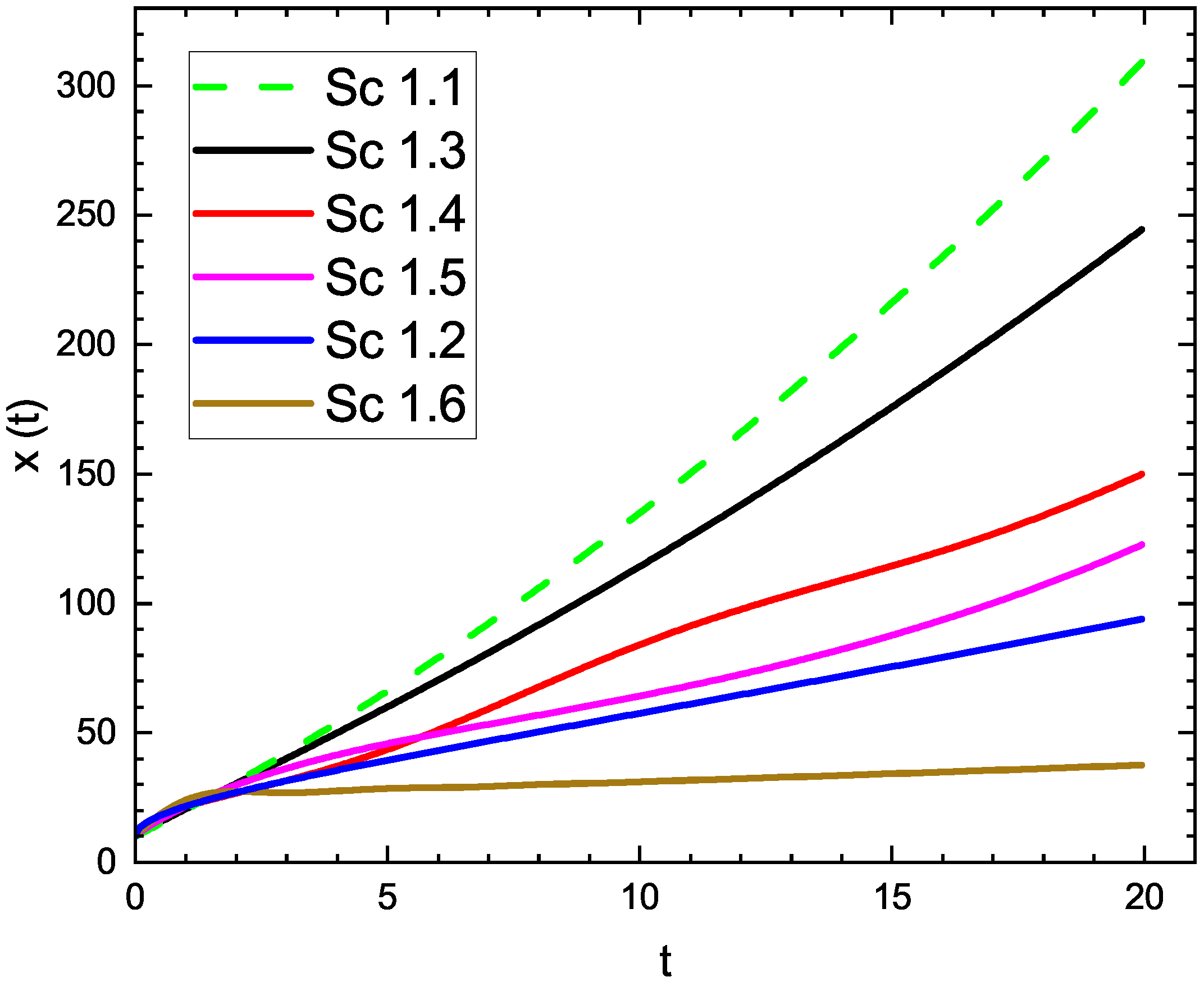
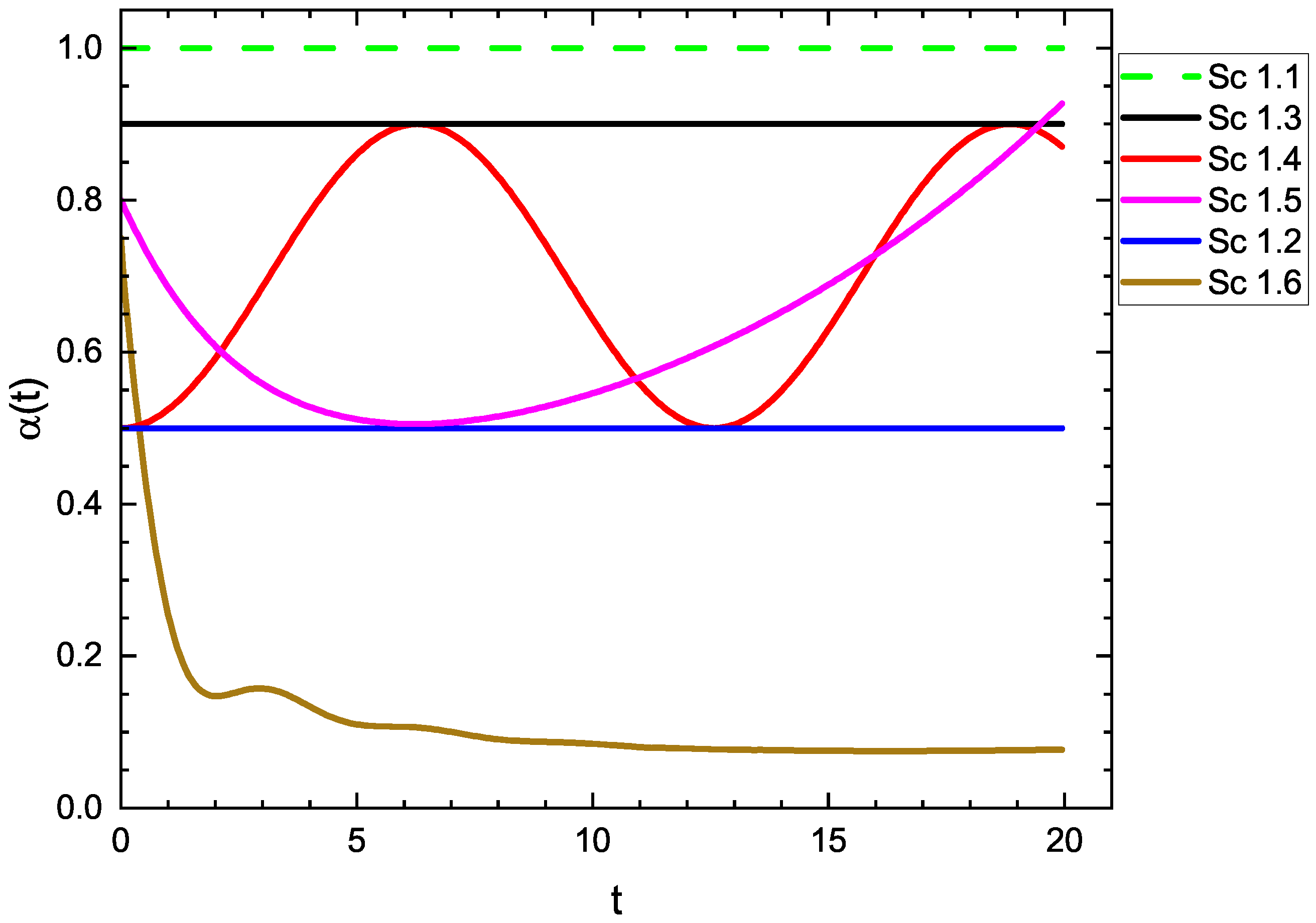
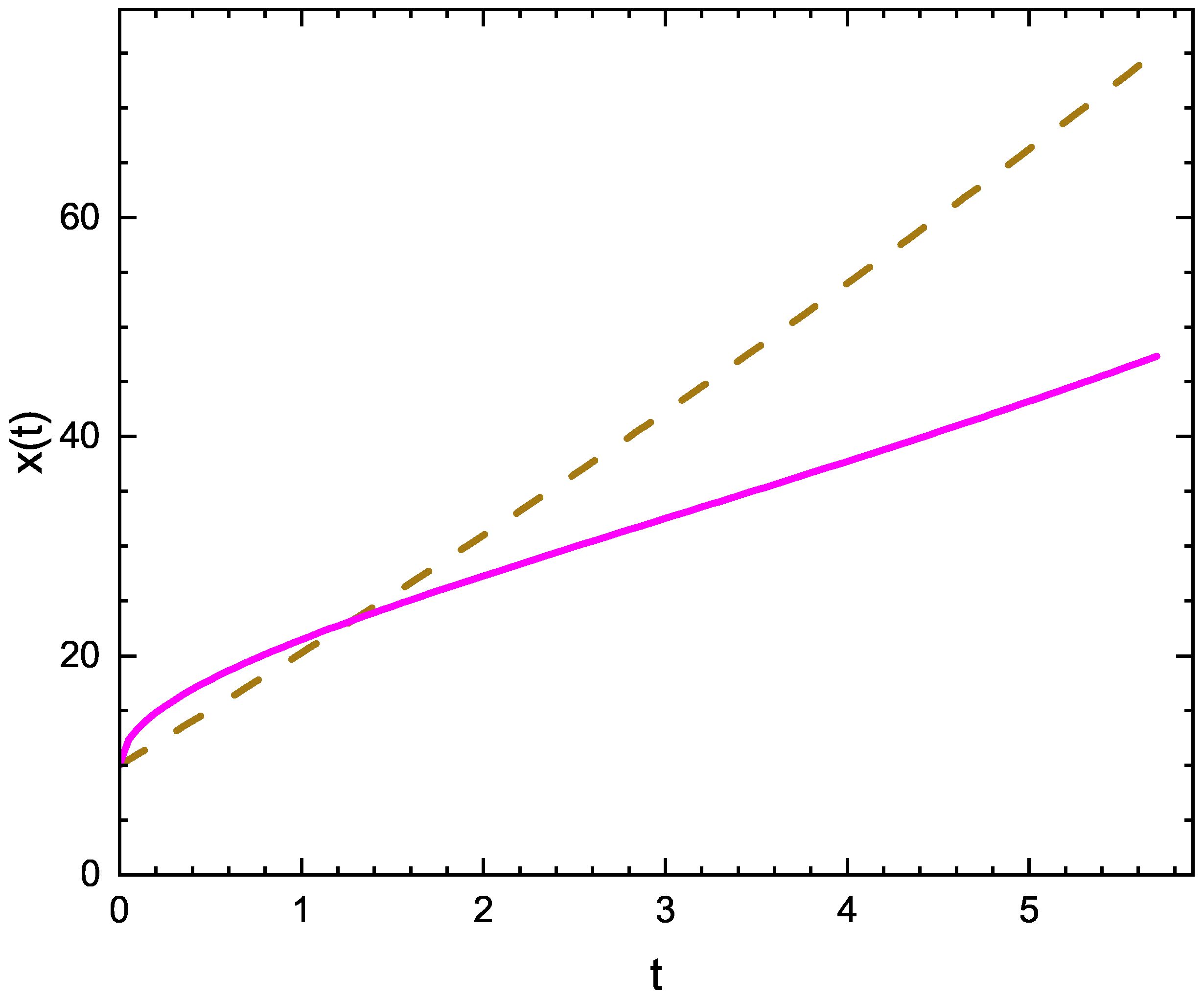
The inverse Laplace transform of Equation (15) was obtained by using the Talbot numerical method [5]. It is worth noting that the parameters and functions in Table 1 were selected ad hoc to avoid stability and convergence issues with the Talbot method. Furthermore, this method is easy to implement and highly reliable, as suggested by Garrappa et al. [15]’s recommendations on the use of inverse Laplace transform techniques to address problems involving Scarpi derivatives. Figure 1 shows the solutions for $x\left(t\right)$ according to the six sub-cases compiled in Table 1. The dashed curve corresponds to the classical integer-order model, $\alpha =1$, which—from a physical point of view—can represent the uniformly accelerated rectilinear motion in “Newtonian” mechanics. The continuous curves for $\alpha$ = 0.5 and 0.9 (sub-cases 1.2 and 1.3, respectively) correspond to the solutions of the system (10) and (11) in terms of fractional Caputo derivative operators, which physically could represent anomalous behavior (deviations) of the classical dynamics. However, this interpretation is not explored in detail in this paper, as it exceeds the scope of the present work. The curve corresponding to sub-case 1.4 was obtained for a pre-specified cosine function that describes the time evolution of the fractional order $\alpha$. Low amplitude fluctuations in $x\left(t\right)$ can be observed, indicating a sort of memory effect in which the oscillations defining the behavior of $\alpha \left(t\right)$ have been propagated to a certain degree in the solution curve; something similar has been found recently in [25]. It is worth mentioning that the use of pre-established functions to define the temporal behavior of $\alpha$ using the Scarpi derivative has already been explored in [15] where exponential and Mittag–Leffler-type transition functions were used to define $\alpha \left(t\right)$. However, it is only very recently that a type of dynamics of the variable order $\alpha$ has been proposed in terms of differential equations [17], with $\alpha$ and t as the dependent and independent variables, respectively. In sub-cases 1.5 and 1.6, we have considered dynamics for $\alpha$ in terms of a first-order differential equation in which we have also included the state variable $x\left(t\right)$, as in sub-case 1.5, and the state variable $x\left(t\right)$ and its ordinary first derivative $\dot{x}\left(t\right)$, as in sub-case 1.6. These last two sub-cases, to our knowledge, represent a novelty, since dynamics for $\alpha$ have been separately explored exclusively in terms of the state variables in [19] and dynamics for $\alpha$ have been proposed exclusively in terms of a differential equation composed of $\alpha$ and its first derivative [17]. In Figure 2, the different behaviors of $\alpha \left(t\right)$ for the considered sub-cases are shown. One key point to emphasize in sub-cases 1.5 and 1.6 is that the dynamics of $\alpha$ affect the dynamics of x and vice versa. An additional aspect to consider is that the values of $\alpha \left(t\right)$ in Figure 2 are bounded such that they can only vary between 0 and 1. This restriction can be imposed, for example, by the physical characteristics dictated by the analyzed problem. However, by setting limits on $\alpha$, it also restricts the possible number of solutions. Thus, solving sub-cases 1.5 and 1.6 involves search problems within the parameter space $\mathcal{P}=\{(ϵ,b,c,d)\in {\mathbb{R}}^4\}$ so that it holds $\alpha :\mathbb{R}\to [0,1],t\in \mathbb{R}.$

3.2. Case 2

$${}^{S}D_0^{\alpha \left(t\right)}x\left(t\right)=v_0+at$$

(16)

$$\ddot{\alpha }\left(t\right)+{}^{C}D_0^{\kappa }\alpha \left(t\right)+b\alpha \left(t\right)+cx\left(t\right)=0$$

(17)

After applying the Laplace transform to Equations (16) and (17), the following results are obtained, respectively:

$$A\left(s\right)={\displaystyle \frac{{\alpha }^{\prime }\left(0\right)-cX\left(s\right)+\alpha \left(0\right)s^{\kappa -1}+\alpha \left(0\right)s}{b+s^{\kappa }+s^2}}$$

(18)

$$s^{sA\left(s\right)}X\left(s\right)-s^{sA\left(s\right)-1}x\left(0\right)={\displaystyle \frac{a}{s^2}}+{\displaystyle \frac{v_0}{s}}$$

(19)

The system of algebraic Equations (18) and (19) has the following exact solution in terms of the Lambert $W(·)$ function, see Appendix A:

$$X\left(s\right)={\displaystyle \frac{x\left(0\right)}{s}}-{\displaystyle \frac{\left(b+s^{\kappa }+s^2\right)W\left(-\frac{cln\left(s\right)\left(a+s{v}_0\right)s^{\frac{b\alpha \left(0\right)+cx\left(0\right)-s{\alpha }^{\prime }\left(0\right)}{b+s^{\kappa }+s^2}-1-\alpha \left(0\right)}}{b+s^{\kappa }+s^2}\right)}{csln\left(s\right)}}$$

(20)

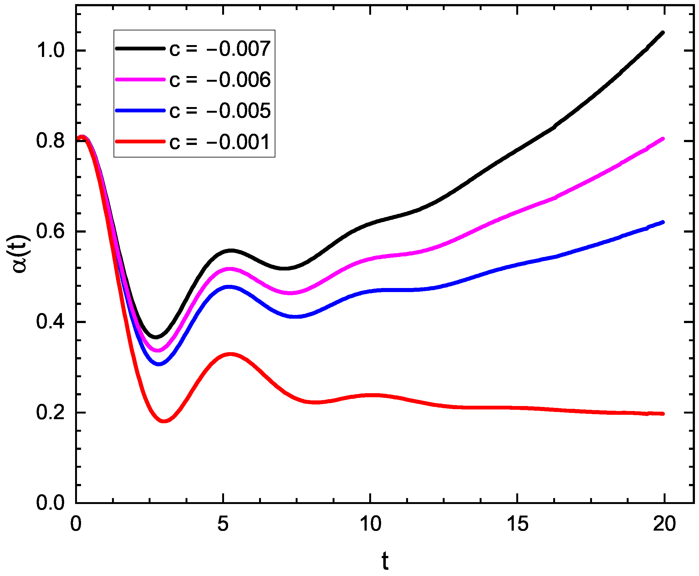
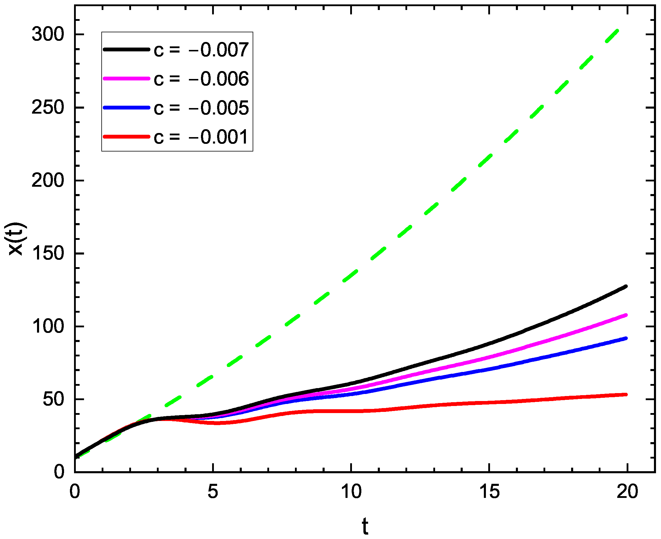
In this case, dynamics for $\alpha \left(t\right)$ are proposed in terms of an equation that combines a second-order ordinary derivative with a Caputo derivative and also include the state variable $x\left(t\right)$. The first three terms of Equation (7) set to zero represent the famous Bagley–Torvik equation [26], which is used, among other things, to model the motion of a rigid plate in a viscous fluid. For the chosen values of the parameters b and c, attenuated oscillatory behaviors for $\alpha \left(t\right)$ are obtained (see Figure 3). These behaviors, in turn, propagate through the solution curves $x\left(t\right)$ in the form of low-amplitude fluctuations, as shown in Figure 4, following the same attenuation period of approximately 15 time units; all of which can be interpreted as a long-period memory effect [25].

3.3. Case 3

$${}^{S}D_0^{\alpha \left(t\right)}x\left(t\right)=v_0+at$$

(21)

$${}^{S}D_0^{\beta \left(t\right)}\alpha \left(t\right)+cx\left(t\right)=0$$

(22)

$${}^{S}D_0^{\gamma \left(t\right)}\beta \left(t\right)+d=0$$

(23)

$$\dot{\gamma }\left(t\right)+e=0$$

(24)

After applying the Laplace transform to Equation (24) the following is obtained:

$$\Gamma \left(s\right)={\displaystyle \frac{s\gamma \left(0\right)-e}{s^2}}$$

(25)

Substituting Equation (25) into the result of applying the Laplace transform to Equation (23), and then solving for $B\left(s\right)$, yields the following:

$$B\left(s\right)={\displaystyle \frac{\beta \left(0\right)-d{s}^{\frac{e}{s}-\gamma \left(0\right)}}{s}}$$

(26)

Substituting Equation (26) into the result of applying the Laplace transform to Equation (22) and then solving for $A\left(s\right)$ results in the following:

$$A\left(s\right)={\displaystyle \frac{\alpha \left(0\right)}{s}}-cX\left(s\right)s^{d{s}^{{\displaystyle \frac{e}{s}}-\gamma \left(0\right)}-\beta \left(0\right)}$$

(27)

Substituting Equation (27) into the result of applying the Laplace transform to Equation (21) and then solving for $X\left(s\right)$ yields:

$$X\left(s\right)s^{s\left({\displaystyle \frac{\alpha \left(0\right)}{s}}-cX\left(s\right)s^{d{s}^{{\displaystyle \frac{e}{s}}-\gamma \left(0\right)}-\beta \left(0\right)}\right)}-x\left(0\right)s^{s\left({\displaystyle \frac{\alpha \left(0\right)}{s}}-cX\left(s\right)s^{d{s}^{{\displaystyle \frac{e}{s}}-\gamma \left(0\right)}-\beta \left(0\right)}\right)-1}={\displaystyle \frac{a}{s^2}}+{\displaystyle \frac{v_0}{s}}$$

(28)

$$X\left(s\right)=\left(a+s{v}_0\right)s^{-\alpha \left(0\right)+cX\left(s\right)s^{-\beta \left(0\right)+d{s}^{{\displaystyle \frac{e}{s}}-\gamma \left(0\right)}+1}-2}+{\displaystyle \frac{x\left(0\right)}{s}}$$

(29)

$$X\left(s\right)={\displaystyle \frac{x_0-\frac{s^{\beta \left(0\right)-d{s}^{\frac{e}{s}-\gamma \left(0\right)}}W\left(-clog\left(s\right)\left(a+s{v}_0\right)s^{-\alpha \left(0\right)-\beta \left(0\right)+cx\left(0\right)s^{d{s}^{\frac{e}{s}-\gamma \left(0\right)}-\beta \left(0\right)}+d{s}^{\frac{e}{s}-\gamma \left(0\right)}-1}\right)}{clog\left(s\right)}}{s}}$$

(30)

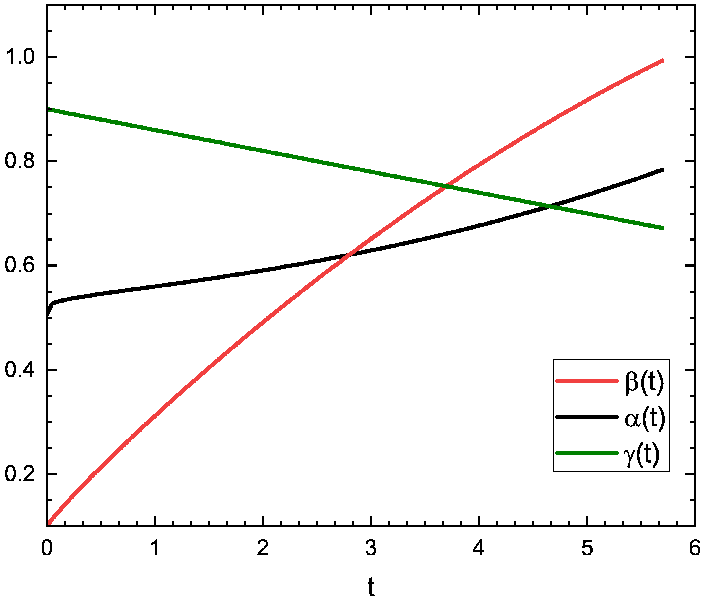
In Case 3, a system has been defined in which the dynamics of $\alpha \left(t\right)$ are described in terms of a Scarpi derivative of variable-order $\beta \left(t\right)$. However, the order $\beta$ exhibits in turn dynamics defined by a Scarpi derivative of order $\gamma \left(t\right)$. Thus, Case 3 poses a recursive process. To our knowledge, this iterative process has not been reported in the literature and offers a promising approach for modeling dynamic systems. Figure 5 shows the solutions for $x\left(t\right)$ belonging to the classical (dashed line) and recursive (solid line) cases. There are clear differences between the two models. Figure 6 shows the temporal evolution of each of the three orders $\alpha$, $\beta$, and $\gamma$. As expected, having a system with three Scarpi derivatives (with their respective variable order) implies more restrictions in the solution search process than the one shown and discussed before in relation to Case 1. An important point to highlight is that the dynamics of $\alpha$, $\beta$, and $\gamma$ affect the dynamic behavior of $x\left(t\right)$ and this influence is mutual.

In the following, we present a result that generalizes Case 3.

Lemma 1. 

Assume a recurrent structure for the dynamic orders of the Scarpi derivatives of the following equation:

$$\begin{array}{cc}\hfill {}^{S}D^{{\alpha }_1\left(t\right)}x\left(t\right)& ={\upsilon }_0+at\hfill \\ \hfill {}^{S}D^{{\alpha }_2\left(t\right)}{\alpha }_1\left(t\right)& =-c_{2}x\left(t\right)\hfill \\ \hfill & ⋮\hfill \\ \hfill {}^{S}D^{{\alpha }_{n-1}\left(t\right)}{\alpha }_{n-2}\left(t\right)& =-c_{n}x\left(t\right)\hfill \\ \hfill {}^{S}D^{{\alpha }_n\left(t\right)}{\alpha }_{n-1}\left(t\right)& =-d\hfill \\ \hfill {\dot{\alpha }}_n\left(t\right)& =-e\hfill \end{array}$$

(31)

where ${\upsilon }_0,a,c_2,\dots ,c_n,d,e$ are positive constants and suppose all the initial conditions. Then, performing the full recursive inverse dynamics for the equation ${}^{S}D^{{\alpha }_1\left(t\right)}x\left(t\right)={\upsilon }_0+at$ in the domain of the Laplace transform, we obtain the following:

$$X\left(s\right)=s^{s^{s^{{·}^{{·}^{{·}^{s^{s^{d{s}^{{\displaystyle \frac{e}{s}}}}{c}_{n}X\left(s\right)-1}{c}_{n-1}X\left(s\right)-1c_{n-2}X\left(s\right)-1_{\ddots c_{3}X\left(s\right)-1}}}}}}{c}_{2}sX\left(s\right)}\left({\displaystyle \frac{{\upsilon }_0}{s}}+{\displaystyle \frac{a}{s^2}}\right)+{\displaystyle \frac{x\left(0\right)}{s}}.$$

(32)

Proof. 

Applying the Laplace transform to each equation, we obtain

$$\begin{array}{cc}\hfill s^{s{A}_1\left(s\right)}X\left(s\right)-s^{s{A}_1\left(s\right)-1}x\left(0\right)& ={\displaystyle \frac{{\upsilon }_0}{s}}+{\displaystyle \frac{a}{s^2}}\hfill \\ \hfill s^{s{A}_2\left(s\right)}{A}_1\left(s\right)-s^{s{A}_2\left(s\right)-1}{\alpha }_1\left(0\right)& =-c_{2}X\left(s\right)\hfill \\ \hfill & ⋮\hfill \\ \hfill s^{s{A}_{n-1}\left(s\right)}{A}_{n-2}\left(s\right)-s^{s{A}_{n-1}\left(s\right)-1}{\alpha }_{n-2}\left(0\right)& =-c_{n}X\left(s\right)\hfill \\ \hfill s^{s{A}_n\left(s\right)}{A}_{n-1}\left(s\right)-s^{s{A}_n\left(s\right)-1}{\alpha }_{n-1}\left(0\right)& =-{\displaystyle \frac{d}{s}}\hfill \\ \hfill s{A}_n\left(s\right)-{\alpha }_n\left(0\right)& =-{\displaystyle \frac{e}{s}}\hfill \end{array}$$

(33)

We now proceed to make the recursive substitutions in inverse sequence; for simplicity, we suppose all the initial conditions. We then use mathematical induction to obtain the result

$$\begin{array}{cc}\hfill s^{-{\displaystyle \frac{e}{s}}}{A}_{n-1}\left(s\right)& =-{\displaystyle \frac{d}{s}}\hfill \\ \hfill A_{n-1}\left(s\right)& =-d{s}^{{\displaystyle \frac{e}{s}}-1}\hfill \\ \hfill s^{-d{s}^{{\displaystyle \frac{e}{s}}}}{A}_{n-2}\left(s\right)& =-c_{n}X\left(s\right)\hfill \\ \hfill A_{n-2}\left(s\right)& =-s^{d{s}^{{\displaystyle \frac{e}{s}}}}{c}_{n}X\left(s\right)\hfill \\ \hfill s^{s{A}_{n-2}\left(s\right)}{A}_{n-3}\left(s\right)& =-c_{n-1}X\left(s\right)\hfill \\ \hfill s^{-s^{d{s}^{{\displaystyle \frac{e}{s}}}}{c}_{n}X\left(s\right)+1}{A}_{n-3}\left(s\right)& =-c_{n-1}X\left(s\right)\hfill \\ \hfill A_{n-3}\left(s\right)& =-s^{s^{d{s}^{{\displaystyle \frac{e}{s}}}}{c}_{n}X\left(s\right)-1}{c}_{n-1}X\left(s\right)\hfill \\ \hfill s^{-s^{s^{d{s}^{{\displaystyle \frac{e}{s}}}}{c}_{n}X\left(s\right)-1}{c}_{n-1}X\left(s\right)+1}{A}_{n-4}\left(s\right)& =-c_{n-2}X\left(s\right)\hfill \\ \hfill A_{n-4}\left(s\right)& =-s^{s^{s^{d{s}^{{\displaystyle \frac{e}{s}}}}{c}_{n}X\left(s\right)-1}{c}_{n-1}X\left(s\right)-1}{c}_{n-2}X\left(s\right)\hfill \\ \hfill s^{s{A}_{n-4}\left(s\right)}{A}_{n-5}\left(s\right)& =-c_{n-3}X\left(s\right)\hfill \\ \hfill s^{-s^{s^{s^{d{s}^{{\displaystyle \frac{e}{s}}}}{c}_{n}X\left(s\right)-1}{c}_{n-1}X\left(s\right)-1}{c}_{n-2}X\left(s\right)+1}{A}_{n-5}\left(s\right)& =-c_{n-3}X\left(s\right)\hfill \\ \hfill A_{n-5}\left(s\right)& =-s^{s^{s^{s^{d{s}^{{\displaystyle \frac{e}{s}}}}{c}_{n}X\left(s\right)-1}{c}_{n-1}X\left(s\right)-1}{c}_{n-2}X\left(s\right)-1}{c}_{n-3}X\left(s\right)\hfill \\ \hfill & ⋮\hfill \\ \\ \hfill A_1\left(s\right)& =-s^{s^{{·}^{{·}^{{·}^{s^{s^{d{s}^{{\displaystyle \frac{e}{s}}}}{c}_{n}X\left(s\right)-1}{c}_{n-1}X\left(s\right)-1c_{n-2}X\left(s\right)-1_{\ddots c_{3}X\left(s\right)-1}}}}}}{c}_{2}X\left(s\right)\hfill \\ \\ \hfill s^{s{A}_1\left(s\right)}X\left(s\right)-s^{s{A}_1\left(s\right)-1}x\left(0\right)& ={\displaystyle \frac{{\upsilon }_0}{s}}+{\displaystyle \frac{a}{s^2}}\hfill \end{array}$$

(34)

$$\begin{array}{cc}\hfill s^{-s^{s^{{·}^{{·}^{{·}^{s^{s^{d{s}^{{\displaystyle \frac{e}{s}}}}{c}_{n}X\left(s\right)-1}{c}_{n-1}X\left(s\right)-1c_{n-2}X\left(s\right)-1_{\ddots c_{3}X\left(s\right)-1}}}}}}{c}_{2}X\left(s\right)+1}X\left(s\right)& =\hfill \\ \hfill \left({\displaystyle \frac{{\upsilon }_0}{s}}+{\displaystyle \frac{a}{s^2}}\right)+s^{-s^{s^{{·}^{{·}^{{·}^{s^{s^{d{s}^{{\displaystyle \frac{e}{s}}}}{c}_{n}X\left(s\right)-1}{c}_{n-1}X\left(s\right)-1c_{n-2}X\left(s\right)-1_{\ddots c_{3}X\left(s\right)-1}}}}}}{c}_{2}X\left(s\right)}x\left(0\right)\end{array}$$

(35)

$$\begin{array}{cc}\hfill X\left(s\right)& =\hfill \\ \hfill s^{s^{s^{{·}^{{·}^{{·}^{s^{s^{d{s}^{{\displaystyle \frac{e}{s}}}}{c}_{n}X\left(s\right)-1}{c}_{n-1}X\left(s\right)-1c_{n-2}X\left(s\right)-1_{\ddots c_{3}X\left(s\right)-1}}}}}}{c}_{2}X\left(s\right)+1}\left({\displaystyle \frac{{\upsilon }_0}{s}}+{\displaystyle \frac{a}{s^2}}\right)+{\displaystyle \frac{x\left(0\right)}{s}}.\end{array}$$

(36)

□

4. Conclusions

This article presents new approaches for defining the dynamics of variable order in Scarpi’s fractional derivatives, aiming to expand their potential without delving into the physical implications. The key contributions in the three case studies are as follows:

(1)

The first case introduces a new dynamic for $\alpha \left(t\right)$, described by a first-order differential equation that includes the state variable $x\left(t\right)$ and its derivative $\dot{x}\left(t\right)$, which, to our knowledge, has not been previously explored.

(2)

The second case proposes a second-order dynamic for $\alpha \left(t\right)$, combining ordinary and fractional derivatives with the state variable $x\left(t\right)$, illustrating the use of different types of derivatives in defining variable order dynamics.

(3)

The third case presents a recursive system involving variable orders $\alpha \left(t\right)$, $\beta \left(t\right)$, and $\gamma \left(t\right)$, which interact and influence each other. This novel approach has not yet been addressed in the literature and contrasts significantly with traditional models. In addition, a Lemma generalizing the third case is presented.

This study used the Talbot method for Laplace transform inversion to solve models with variable-order dynamics, emphasizing feasibility over detailed numerical analysis. While numerical accuracy, stability, and convergence are important, a thorough evaluation was not within the scope of this work. Future research could focus on comparing the Talbot method with other inversion techniques to enhance numerical accuracy, stability, and reliability in solving problems with variable-order derivatives, contributing to a deeper understanding of computational methods in this field.

Variable-order dynamics fill gaps in existing models by allowing the derivative order to vary over time according to an underlying dynamic process rather than being predefined by a fixed function or restricted to fixed integer or fractional orders, as in most studies in the literature so far. It is crucial to emphasize that in all three cases studied, the dynamics defining the behavior of $\alpha \left(t\right)$ are coupled with the model that contains the state variable $x\left(t\right)$ and its derivatives. This aspect is entirely novel and, to the best of our knowledge, has not been explored before. Expanding the use of Scarpi derivatives requires the development of implicit numerical schemes to perform the Laplace inverse transform. This would eliminate the need to solve Equations (14), (19) and (28) for $X\left(s\right)$ exactly or approximately, followed by performing the inverse transform using an explicit numerical scheme like the Talbot method. The implicit schemes would allow for the exploration of more complex linear models beyond the one represented by Equation (10). Moreover, it is necessary to investigate dynamic systems associated with various applications (such as modeling biological systems, forecasting financial markets, and controlling dynamic systems in engineering, to mention a few), incorporating Scarpi derivatives. Such systems could involve dynamics similar to those we have proposed or variations thereof. However, this poses two challenges: First, the use of variable-order dynamics must be justified. Second, additional work will be needed to understand its implications and interpretations within the context of the specific application being modeled. On the other hand, imposing limits on the order of the Scarpi derivative restricts the number of solutions to the study system, which involves the problem of searching for relevant parameters. It is necessary to find combinations of values that satisfy the imposed limits and the solution domain of interest. This approach opens new research avenues related not only to parameter search but also to system stability, among other aspects. To conclude, it is important to recognize the weaknesses of the present study, which include the lack of detailed numerical analysis, the absence of comparisons with other methods, and the need for a clearer justification in specific applications. Additionally, scalability to complex nonlinear systems requires further investigation. The key premises underlying this study are as follows: The solutions, while not exact, are precise and reliable. However, no rigorous numerical analysis was performed. We assume that the variable-order range is between [0, 1], although it could be extended. We assume that the systems’ dynamics are complex, though we did not formally assess this using dynamic system theory tools such as Lyapunov exponents. Future work should address these aspects to reduce the reliance on unverified assumptions.

References

- Feng, X.; Sutton, M. A new theory of fractional differential calculus. Anal. Appl. 2021, 19, 715–750. [Google Scholar] [CrossRef]
- Ostalczyk, P.; Sankowski, D.; Nowakowski, J. Non-Integer Order Calculus and its Applications: 9th International Conference on Non-Integer Order Calculus and its Applications, Łódź, Poland; Springer: Cham, Switerland, 2018. [Google Scholar] [CrossRef]
- Patnaik, S.; Hollkamp, J.P.; Semperlotti, F. Applications of variable-order fractional operators: A review. Proc. R. Soc. A Math. Phys. Eng. Sci. 2020, 476. [Google Scholar] [CrossRef] [PubMed]
- Sun, H.; Chang, A.; Zhang, Y.; Chen, W. A review on variable-order fractional differential equations: Mathematical foundations, physical models, numerical methods and applications. Fract. Calc. Appl. Anal. 2019, 22, 27–59. [Google Scholar] [CrossRef]
- Polo-Labarrios, M.; Godínez, F.; Quezada-García, S. Numerical-analytical solutions of the fractional point kinetic model with Caputo derivatives. Ann. Nucl. Energy 2022, 166, 108745. [Google Scholar] [CrossRef]
- García-Aspeitia, M.A.; Fernandez-Anaya, G.; Hernández-Almada, A.; Leon, G.; Magaña, J. Cosmology under the fractional calculus approach. Mon. Not. R. Astron. Soc. 2022, 517, 4813–4826. [Google Scholar] [CrossRef]
- Zhou, Y.; Wang, J.; Zhang, L. Basic Theory of Fractional Differential Equations, 2nd ed.; World Scientific: Singapore, 2016. [Google Scholar] [CrossRef]
- Xu, S.; Wang, X.; Ye, X. A new fractional-order chaos system of Hopfield neural network and its application in image encryption. Chaos Solitons Fractals 2022, 157, 111889. [Google Scholar] [CrossRef]
- Ding, W.; Patnaik, S.; Sidhardh, S.; Semperlotti, F. Applications of Distributed-Order Fractional Operators: A Review. Entropy 2021, 23, 110. [Google Scholar] [CrossRef]
- Ayazi, N.; Mokhtary, P.; Moghaddam, B.P. Efficiently solving fractional delay differential equations of variable order via an adjusted spectral element approach. Chaos Solitons Fractals 2024, 181, 114635. [Google Scholar] [CrossRef]
- Almeida, R.; Martins, N.; da C. Sousa, J.V. Fractional tempered differential equations depending on arbitrary kernels. AIMS Math. 2024, 9, 9107–9127. [Google Scholar] [CrossRef]
- Muñoz-Vázquez, A.J.; Eduardo Carvajal-Rubio, J.; Fernández-Anaya, G.; Sánchez-Torres, J.D. Output feedback robust stabilization of distributed-order systems. Asian J. Control. 2025. [Google Scholar] [CrossRef]
- Sousa, J.V.D.C.; Machado, J.T.; De Oliveira, E.C. The ψ-Hilfer fractional calculus of variable order and its applications. Comput. Appl. Math. 2020, 39, 296. [Google Scholar] [CrossRef]
- Scarpi, G. Sulla possibilità di un modello reologico intermedio di tipo evolutivo. Atti Accad. Naz. Lincei. Cl. Sci. Fis. Mat. E Naturali. Rend. 1972, 52, 912–917. [Google Scholar]
- Garrappa, R.; Giusti, A.; Mainardi, F. Variable-order fractional calculus: A change of perspective. Commun. Nonlinear Sci. Numer. Simul. 2021, 102, 105904. [Google Scholar] [CrossRef]
- Garrappa, R.; Giusti, A. A Computational Approach to Exponential-Type Variable-Order Fractional Differential Equations. J. Sci. Comput. 2023, 96, 63. [Google Scholar] [CrossRef]
- Giusti, A.; Colombaro, I.; Garra, R.; Garrappa, R.; Mentrelli, A. On variable-order fractional linear viscoelasticity. Fract. Calc. Appl. Anal. 2024, 27, 1578. [Google Scholar] [CrossRef]
- Lorenzo, C.F.; Hartley, T.T. Variable Order and Distributed Order Fractional Operators. Nonlinear Dyn. 2002, 29, 98. [Google Scholar] [CrossRef]
- Sun, H.-G.; Sheng, H.; Chen, Y.-Q.; Chen, W.; Yu, Z.-B. A Dynamic-Order Fractional Dynamic System. Chin. Phys. Lett. 2013, 30, 046601. [Google Scholar] [CrossRef]
- Horvat, M.A.; Sarajlija, N. On the fractional relaxation equation with Scarpi derivative. arXiv 2024, arXiv:2411.03317. [Google Scholar]
- Han, B.; Yin, D.; Gao, Y. The application of a novel variable-order fractional calculus on rheological model for viscoelastic materials. Mech. Adv. Mater. Struct. 2024, 31, 9951–9963. [Google Scholar] [CrossRef]
- Moghaddam, B.P.; Dabiri, A.; Machado, J.A.T. Application of variable-order fractional calculus in solid mechanics. Appl. Eng. Life Soc. Sci. Part A 2019, 7, 207–224. [Google Scholar]
- Cuesta, E.; Kirane, M.; Alsaedi, A.; Ahmad, B. On the sub–diffusion fractional initial value problem with time variable order. Adv. Nonlinear Anal. 2021, 10, 1301–1315. [Google Scholar] [CrossRef]
- Coimbra, C. Mechanics with variable-order differential operators. Ann. Der Phys. 2003, 515, 692–703. [Google Scholar] [CrossRef]
- Godinez, F.A.; Quezada-Garcia, S.; Fernandez-Anaya, G.; Quezada-Tellez, L.A.; Polo-Labarrios, M.A. Variable-Order Fractional Neutron Point Kinetics Model to Nuclear Reactor. Fractals 2024. [Google Scholar] [CrossRef]
- Atanackovic, T.M.; Zorica, D. On the Bagley–Torvik Equation. J. Appl. Mech. 2013, 80, 041013. [Google Scholar] [CrossRef]
Disclaimer/Publisher’s Note: The statements, opinions and data contained in all publications are solely those of the individual author(s) and contributor(s) and not of MDPI and/or the editor(s). MDPI and/or the editor(s) disclaim responsibility for any injury to people or property resulting from any ideas, methods, instructions or products referred to in the content. |
© 2025 by the authors. Licensee MDPI, Basel, Switzerland. This article is an open access article distributed under the terms and conditions of the Creative Commons Attribution (CC BY) license (https://creativecommons.org/licenses/by/4.0/).