Variable-Fractional-Order Nosé–Hoover System: Chaotic Dynamics and Numerical Simulations

Abstract

This study explores the variable-order fractional Nosé–Hoover system, investigating the evolution of its chaotic and stable states under variable-order derivatives. Variable-order derivatives introduce greater complexity and adaptability into a system’s dynamics. The main objective is to examine these effects through numerical simulations, showcasing how changes in the order function influence a system’s behavior. The variable-order behavior is shown by phase space orbits and time series for various variable orders $\alpha$. We look at how the system acts by using numerical solutions and numerical simulations. The phase space orbits and time series for different $\alpha$ show variable-order effects. The findings emphasize the role of variable-order derivatives in enhancing chaotic behavior, offering novel insights into their impact on dynamical systems.

1. Introduction

Fractional calculus, which is a generalization of the traditional integer-order differentiation and integration to non-integer orders, has gained a lot of interest recently due to its sophisticated capability to model complex dynamical processes with high precision compared to traditional models [1,2]. Fractional-order systems are more practical and simpler to use for modeling various engineering, biological, and physical systems, especially those that show memory effects and long-range dependencies [3,4,5,6].

One of the most fascinating properties of fractional-order systems is that they can produce chaotic behavior, a property that is of immense potential for numerous applications, including secure communication, encryption, signal processing, and biological modeling [7,8,9,10,11]. When you add fractional orders to this system, it becomes even more complex and full of different kinds of interactions. This helps us understand nonlinear events like bifurcations, synchronization, and other complicated behaviors [12,13,14,15]. This addition of fractional-order systems opens up new ways to control and study chaotic systems, giving us a better understanding of how complicated things happen in the real world.

We simulate fractional-order systems to describe their stability, bifurcations, and chaotic behavior. Non-integer-order dynamic systems provide further insights into complex phenomenon behaviors that are usually difficult to analyze using traditional integer-order models. Fractional chaotic systems, in particular, have drawn more attention due to their unique dynamical features and high applicability to practical problems in the fields of secure communication, signal processing, and control systems [10,16,17].

This article investigates the dynamics of fractional systems with time-varying fractional orders, which opens up new possibilities for chaos. By examining these kinds of systems in depth, this paper aims to discover patterns and phenomena that can be utilized to enhance the design and optimization of actual systems, thereby making significant contributions to a wide range of technological and scientific applications [18,19].

The novelty of this study lies in the creation of new dynamic behaviors within fractional chaotic systems, i.e., variable-order derivative ones. Through a study of how dynamic variations in the fractional order affect the system, this study uncovers new insights into the interaction between chaos. Unlike most previous research, which assumed that the order would stay the same over time, this study looks at what happens when the order changes over time, giving a more complete picture of how the system works. This approach highlights the role played by memory effects that vary with time and long-range correlations in the establishment of chaotic phenomena. This study solves these variable-order dynamics, which leads to better modeling and control of complex systems. This means that real-world processes can be described in a more accurate and flexible way [20,21,22,23].

In this study, we simulate and investigate dynamical behavior [24] in a variable-order fractional system [25,26] in the following way:

$$\left\{\begin{array}{cc}\hfill {}_0\mathcal{D}_t^{\alpha \left(t\right)}{x}_1\left(t\right)& =x_2,\hfill \\ \hfill {}_0\mathcal{D}_t^{\alpha \left(t\right)}{x}_2\left(t\right)& =x_2{x}_3-x_1,\hfill \\ \hfill {}_0\mathcal{D}_t^{\alpha \left(t\right)}{x}_3\left(t\right)& =1-x_2^2,.\hfill \end{array}\right.$$

(1)

where $x_1\left(t\right),x_2\left(t\right),$ and $x_3\left(t\right)$ represent the state variables and become chaotic for the initial values $x_1\left(0\right)=0,x_2\left(0\right)=1,$ and $x_3\left(0\right)=0$.

This study investigates the dynamical behaviors of a new chaotic fractional system with variable-order derivatives. The variable-order fractional derivatives have been of recent research interest as a powerful tool for modeling systems with varying memory effects. By examining how such dynamic ordering changes affect chaos, we hope to offer a more profound insight into the impact of fractional dynamics on the unpredictability and stability of systems. This view creates new insights into the complex interactions between fractional-order changes and system behavior, enhancing our analysis and control of chaotic systems.

2. Mathematical Preliminaries

Definition 1

([27,28]). The fractional-order derivative of a function $Q\left(t\right)$ based on the Caputo definition with variable order $\alpha \left(t\right)>0$ is given by

$${}_0{}^{\mathrm{c }}\mathcal{D}^{\alpha \left(t\right)}W\left(t\right)={\displaystyle \frac{1}{\Gamma (n-\alpha (t\left)\right)}}{\int }_0^t{(t-h)}^{n-\alpha \left(t\right)-1}{W}^{\left(n\right)}\left(h\right)dh,t>0.$$

(2)

where $n-1<\alpha \le n,n\in \mathbb{N}$.

Definition 2

([27,28]). The Riemann–Liouville fractional integral of a function $Q:{\mathbb{R}}^{+}\to \mathbb{R}$ of variable order $\alpha \left(t\right)>0$ is defined as

$$J_0^{\alpha \left(t\right)}W\left(t\right)={\displaystyle \frac{1}{\Gamma \left(\alpha \right(t\left)\right)}}{\int }_0^t{(t-h)}^{\alpha \left(t\right)-1}W\left(h\right)dh,t>0.$$

(3)

where $\Gamma (·)$ is the gamma function.

3. Numerical Schemes for Variable-Order Fractional System

When trying to solve differential equations that do not have a closed form, numerical methods are useful. It is harder to solve fractional-order equations because they have derivatives of non-integer orders. Numerous studies have examined Euler’s method, Adams–Bashforth method, Adomian decomposition, homotopy analysis, Laplace–Adomian decomposition, and polynomial interpolation [29,30,31,32].

For efficiency, simple methods like Euler’s one are preferred, and advanced methods like Lagrange two-step interpolation are more precise when resources are available [33,34].

This section focuses on approximating solutions in [35,36] for models using Caputo fractional operators through efficient numerical techniques. The system is as follows:

$${}^{*}D_{0,t}^{\alpha }h\left(t\right)=W\left(h\left(t\right)\right),t\in [0,a],h\left(0\right)=h_0,$$

(4)

where * denotes one of the fractional-order operators under consideration and $h_0$ is the initial state of the system using definition Equation (2).

Consider an equi-spaced mesh over $[0,a]$ with step size $\Delta t=0.05$. Let $h_r$ approximate $h\left(t\right)$ at $t=t_r$. The finite difference scheme for (4) provides the numerical technique for the variable order given by

Variable Order

Using the numerical method in [37], Equation (4) can be reformulated as

$$h\left(t\right)-h\left(0\right)={\displaystyle \frac{1}{\Gamma \left(w\right(t\left)\right)}}{\int }_0^{t}f(R,h\left(R\right)){(t-R)}^{w\left(t\right)-1}dR.$$

(5)

At $t=t_{\mu +1}$, Equation (5) is formulated as follows:

$$h\left(t_{\mu +1}\right)-h\left(0\right)={\displaystyle \frac{1}{\Gamma \left(w\right(t\left)\right)}}\sum _{r=0}^{\mu }{\int }_{t_r}^{t_{r+1}}f(R,h\left(R\right)){(t_{\mu +1}-R)}^{w\left(t\right)-1}dR.$$

(6)

Using the two-step Lagrange polynomial interpolation over the interval $[t_N,t_{N+1}]$, we have

$$M_N\left(R\right)\simeq {\displaystyle \frac{f(t_{\xi },h_{\xi })}{h}}(R-t_{\xi -1})-{\displaystyle \frac{f(t_{\xi -1},h_{\xi -1})}{h}}(R-t_{\xi }).$$

(7)

Now, considering Equations (6) and (7), we have

$$h_{\mu +1}\left(t\right)=h_0+{\displaystyle \frac{1}{\Gamma \left(w\right(t\left)\right)}}\sum _{\xi =0}^{\mu }\left({\displaystyle \frac{f(t_{\xi },h_{\xi })}{h}}{\int }_{t_{\xi }}^{t_{\xi +1}}(t-t_{\xi -1}){(t_{\mu +1}-t)}^{w\left(t\right)-1}dt\right.$$

$$\left.-{\displaystyle \frac{f(t_{\xi -1},h_{\xi -1})}{h}}{\int }_{t_{\xi }}^{t_{\xi +1}}(t-t_{\xi }){(t_{\mu +1}-t)}^{w\left(t\right)-1}dt\right).$$

(8)

Then,

$$A_{w\left(t\right),\xi ,1}=h^{w\left(t\right)+1}{\displaystyle \frac{{(\mu +1-\xi )}^{w\left(t\right)}(\mu -\xi +2+w\left(t\right))-{(\mu -\xi )}^{w\left(t\right)}(\mu -\xi +2+2w\left(t\right))}{w\left(t\right)\Gamma \left(w\right(t)+1)}},$$

(9)

$$A_{w\left(t\right),\xi ,2}=h^{w\left(t\right)+1}{\displaystyle \frac{{(\mu +1-\xi )}^{w\left(t\right)+1}-{(\mu -\xi )}^{w\left(t\right)}(\mu -\xi +1+w\left(t\right))}{w\left(t\right)\Gamma \left(w\right(t)+1)}}.$$

(10)

From Equations (8) and (9), we have

$$h_{\mu +1}\left(t\right)=h\left(0\right)+{\displaystyle \frac{1}{\Gamma \left(w\right(t\left)\right)}}\sum _{\xi =0}^{\mu }\left({\displaystyle \frac{h^{w\left(t\right)}f(t_{\xi },h_{\xi })}{w\left(t\right)\Gamma \left(w\right(t)+1)}}{(\mu +1-\xi )}^{w\left(t\right)}\times (\mu -\xi +2+w\left(t\right))\right.$$

$$-{(\mu -\xi )}^{w\left(t\right)}(\mu -\xi +2+2w\left(t\right))-{\displaystyle \frac{h^{w\left(t\right)}f(t_{\xi -1},h_{\xi -1})}{w\left(t\right)\Gamma \left(w\right(t)+1)}}{(\mu +1-\xi )}^{w\left(t\right)+1}$$

$$\left.-{(\mu -\xi )}^{w\left(t\right)}(\mu -\xi +1+w\left(t\right))\right).$$

(11)

Thus, the solutions are given by

$${hC}_{x_{\mu +1}\left(t\right)}=x_0+{\displaystyle \frac{1}{\Gamma \left(w\right(t\left)\right)}}\sum _{\xi =0}^{\mu }{\displaystyle \frac{h^{w\left(t\right)}{\omega }_1(t_{\xi },x_{\xi },y_{\xi },z_{\xi })}{w\left(t\right)\Gamma \left(w\right(t)+1)}}\times \left({(\mu +1-\xi )}^{w\left(t\right)}\right.$$

$$\left.-{(\mu -\xi )}^{w\left(t\right)}(\mu -\xi +2+2w\left(t\right))\right),$$

(12)

and ${\omega }_1(t,x)=y$.

$${hC}_{y_{\mu +1}\left(t\right)}=y_0+{\displaystyle \frac{1}{\Gamma \left(w\right(t\left)\right)}}\sum _{\xi =0}^{\mu }{\displaystyle \frac{h^{w\left(t\right)}{\omega }_2(t_{\xi },x_{\xi },y_{\xi },z_{\xi })}{w\left(t\right)\Gamma \left(w\right(t)+1)}}\times \left({(\mu +1-\xi )}^{w\left(t\right)}\right.$$

$$\left.-{(\mu -\xi )}^{w\left(t\right)}(\mu -\xi +2+2w\left(t\right))\right),$$

(13)

and ${\omega }_2(t,y)=yz-x$.

$${hC}_{z_{\mu +1}\left(t\right)}=z_0+{\displaystyle \frac{1}{\Gamma \left(w\right(t\left)\right)}}\sum _{\xi =0}^{\mu }{\displaystyle \frac{h^{w\left(t\right)}{\omega }_3(t_{\xi },x_{\xi },y_{\xi },z_{\xi })}{w\left(t\right)\Gamma \left(w\right(t)+1)}}\times \left({(\mu +1-\xi )}^{w\left(t\right)}\right.$$

$$\left.-{(\mu -\xi )}^{w\left(t\right)}(\mu -\xi +2+2w\left(t\right))\right),$$

(14)

and ${\omega }_3(t,z)=1-y^2$.

The finite scheme is designed to efficiently solve variable-order fractional systems by merging Lagrange interpolation and Caputo derivative discretization. The scheme is optimized to solve time-dependent fractional orders with adaptive terms and further enhance the accuracy through two-step polynomial approximations. The scheme also incorporates a structured memory management strategy based on discretized convolution integrals that preserve non-local effects without computational intractability. Further, the pre-computed coefficient recursive expression allows for stable solutions of coupled systems independent of iterative solvers. Though the method is promising in terms of efficiency, a complete analysis of computational performance is left for future work.

4. System Dynamical Analysis

Dynamical analysis reveals the chaos and stability of nonlinear systems. Variable-order fractional derivatives embrace memory effects with a varying order, adding flexibility in modeling complex dynamics. The Nosé–Hoover system, settled as chaotic, is studied here in its variable-order fractional form, which is not yet fully explored. We study its behavior for different $\alpha$ values via numerical simulations, in which phase portraits, time series, and Lyapunov exponents are employed in order–chaos transitions.

Chaos systems without fixed points, usually corresponding to silent attractors, cannot be investigated by conventional methods such as the Shilnikov approach and are generally studied by Lyapunov exponents [38,39]. Although fractional-order chaotic dynamics have been deeply studied [25,40,41], the variable fractional-order Nosé–Hoover system has hardly been studied.

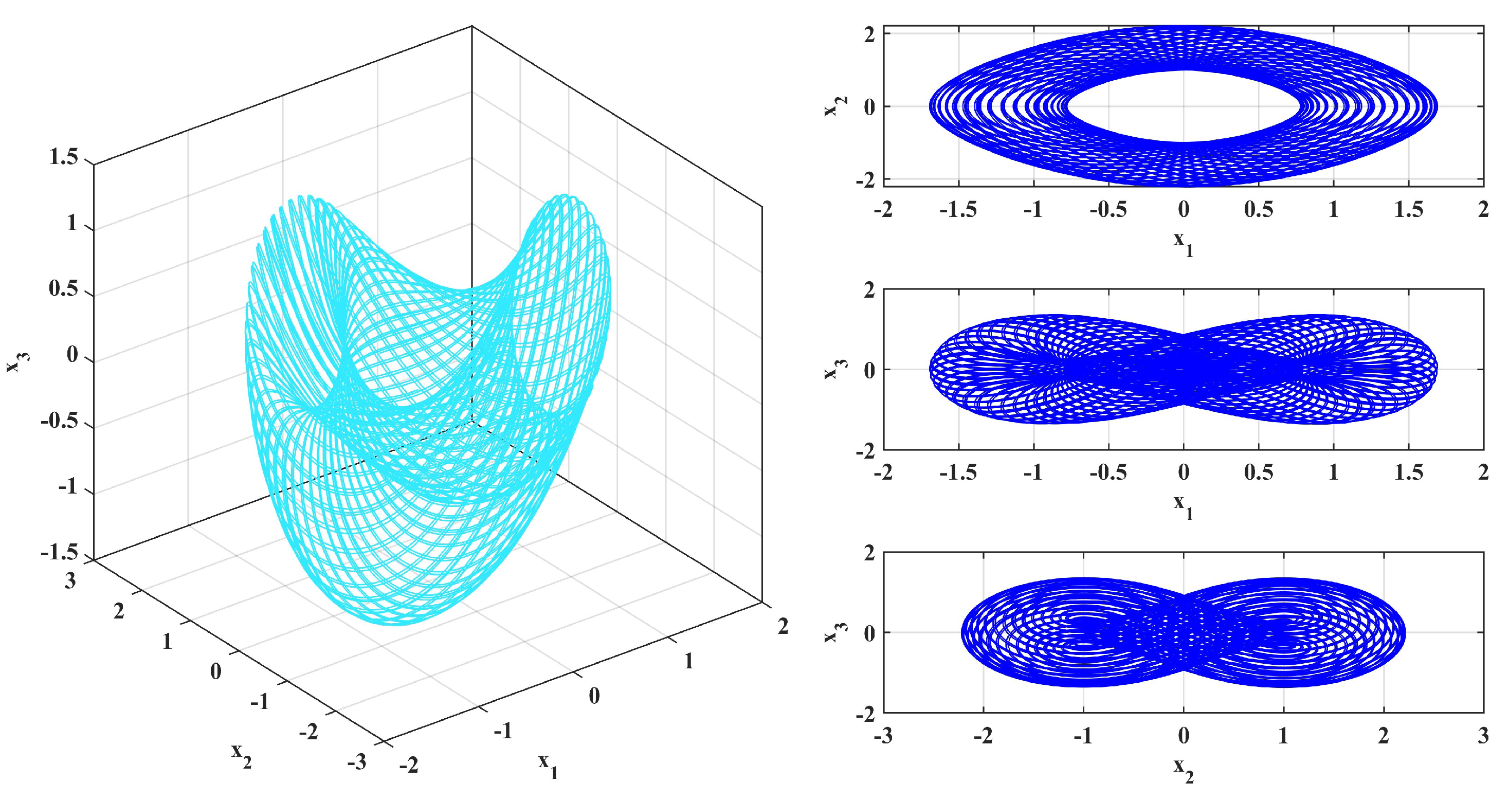
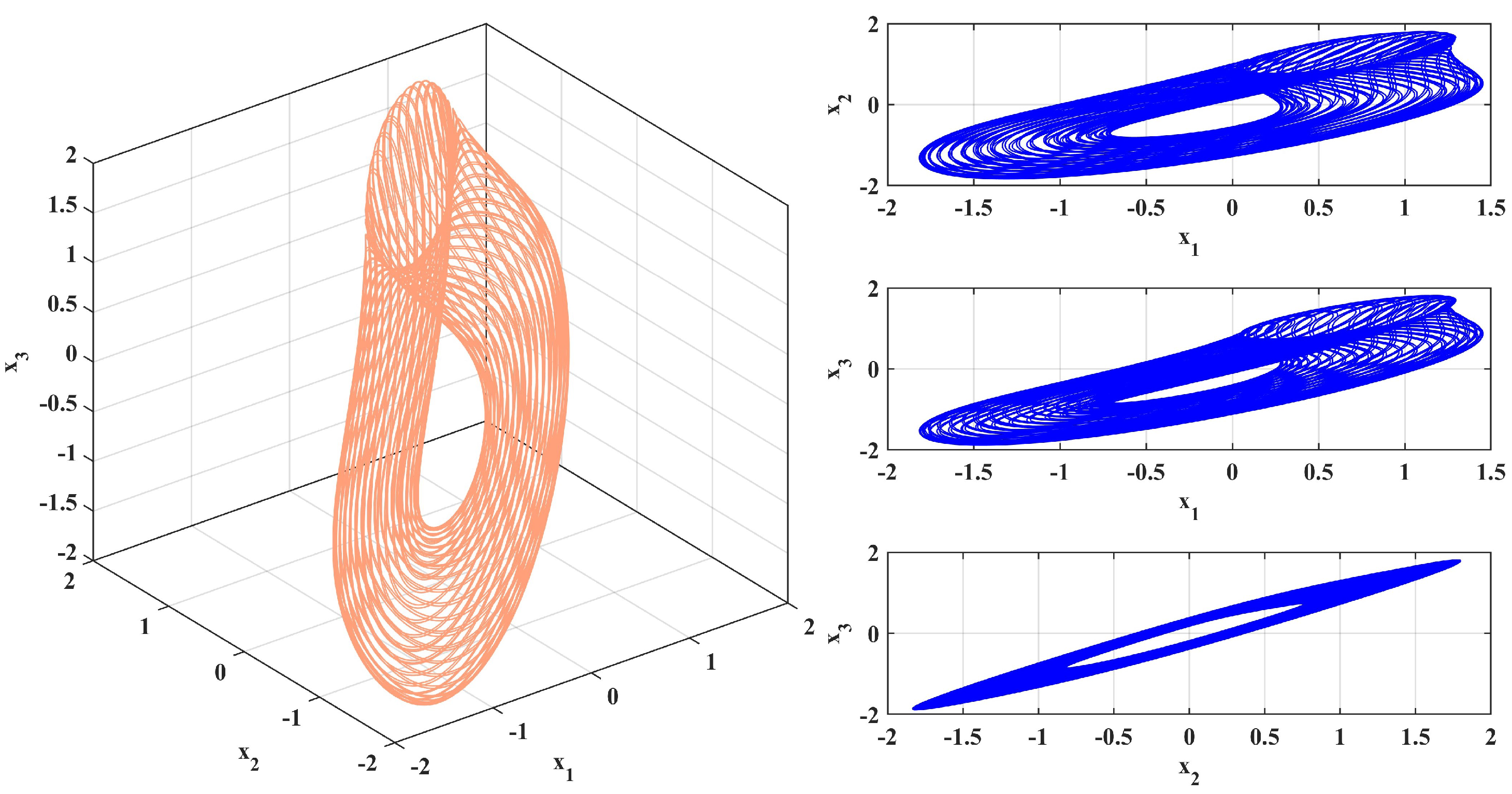
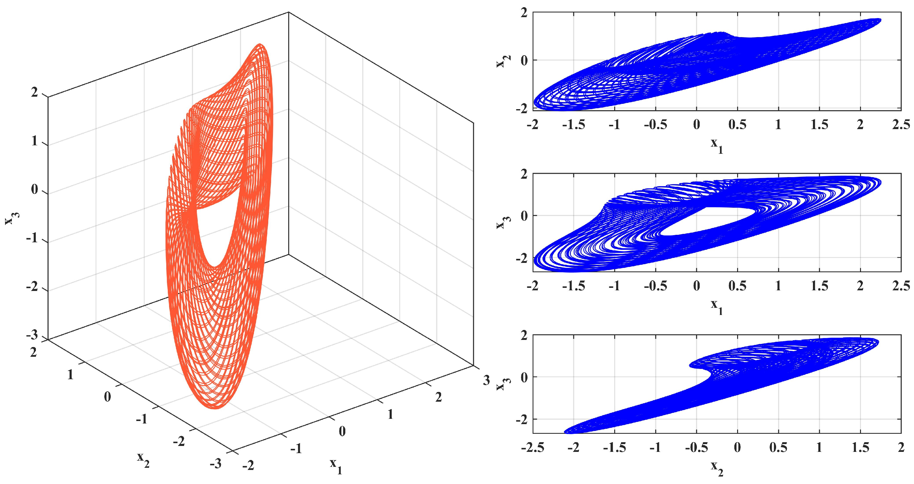
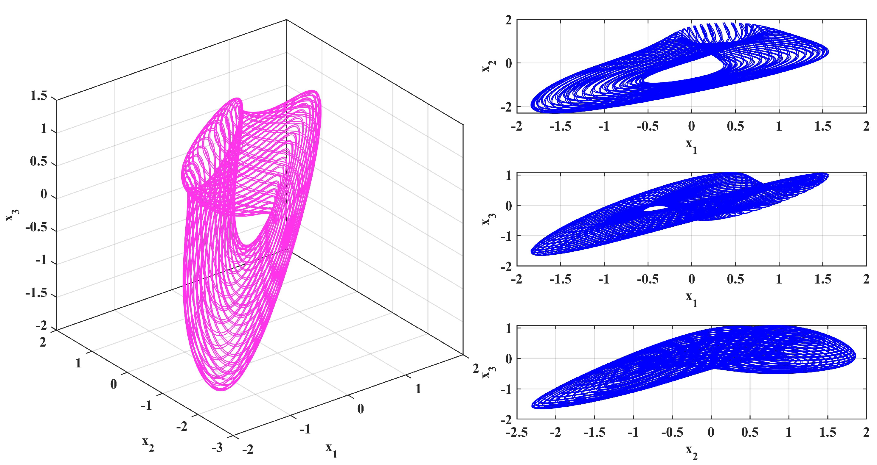
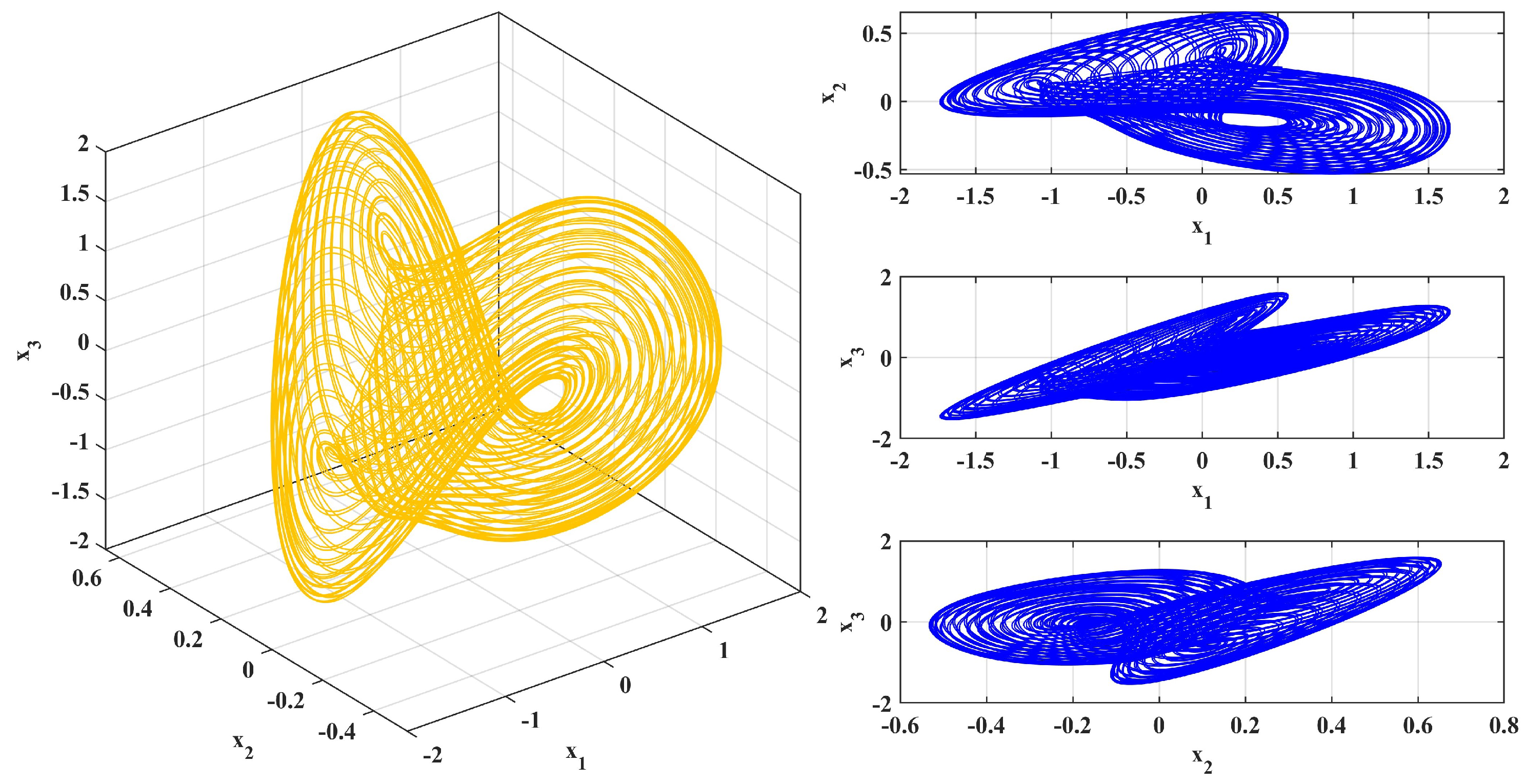
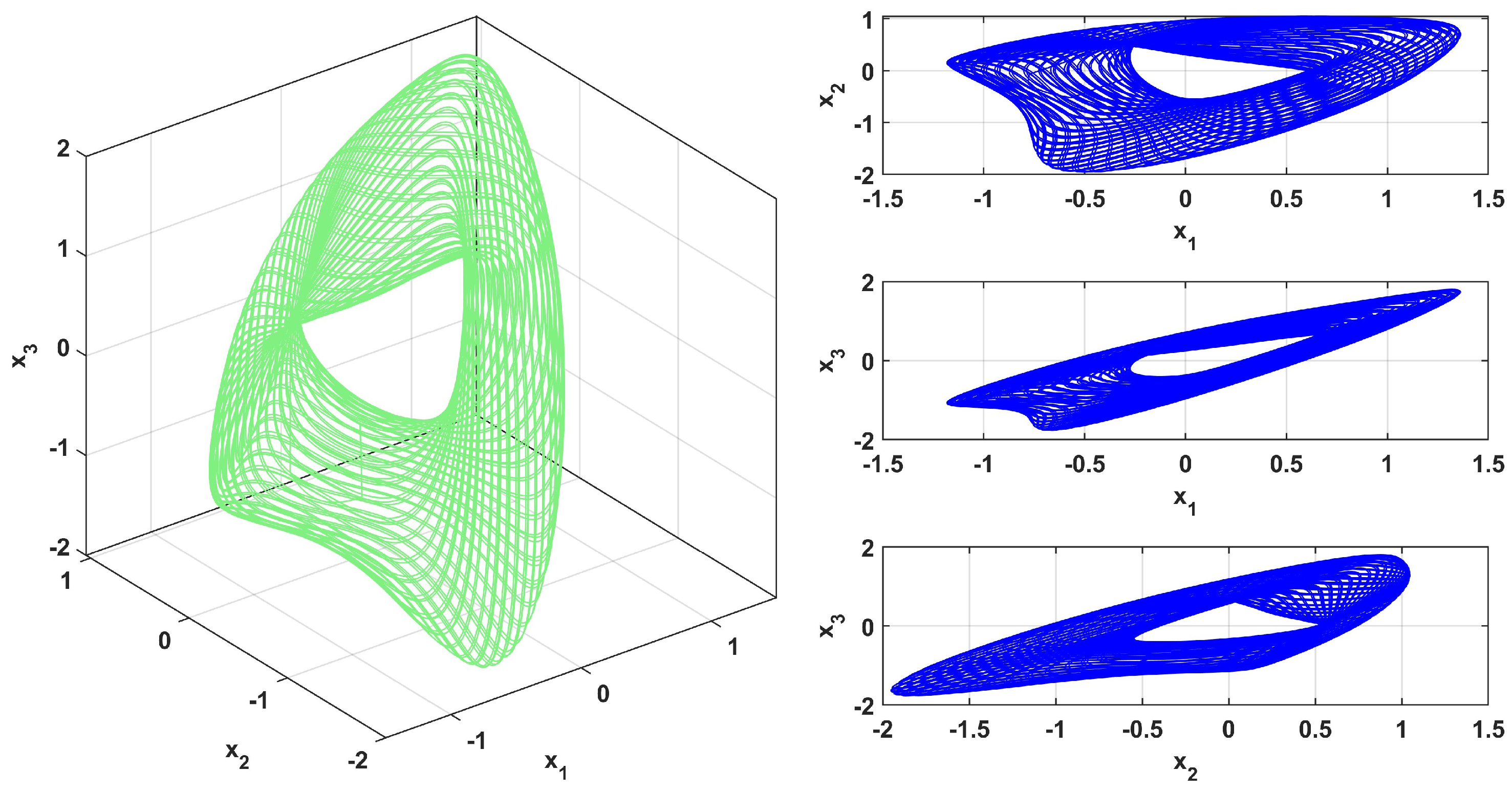
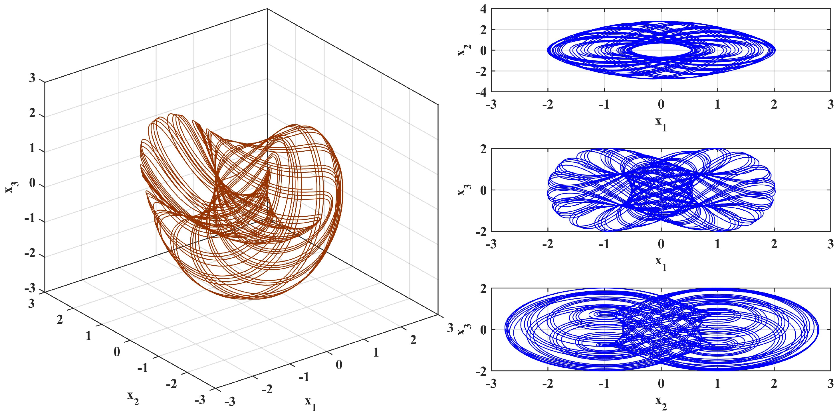
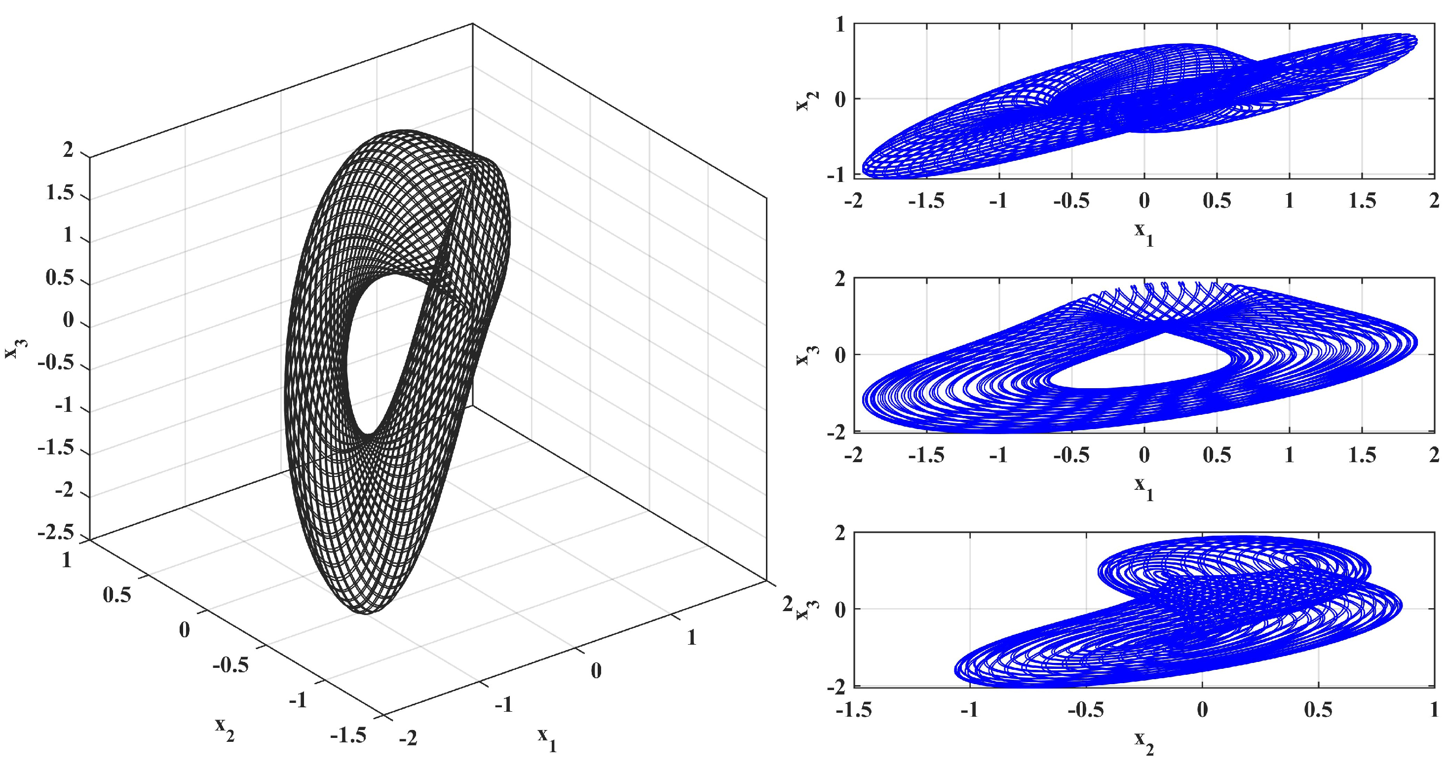
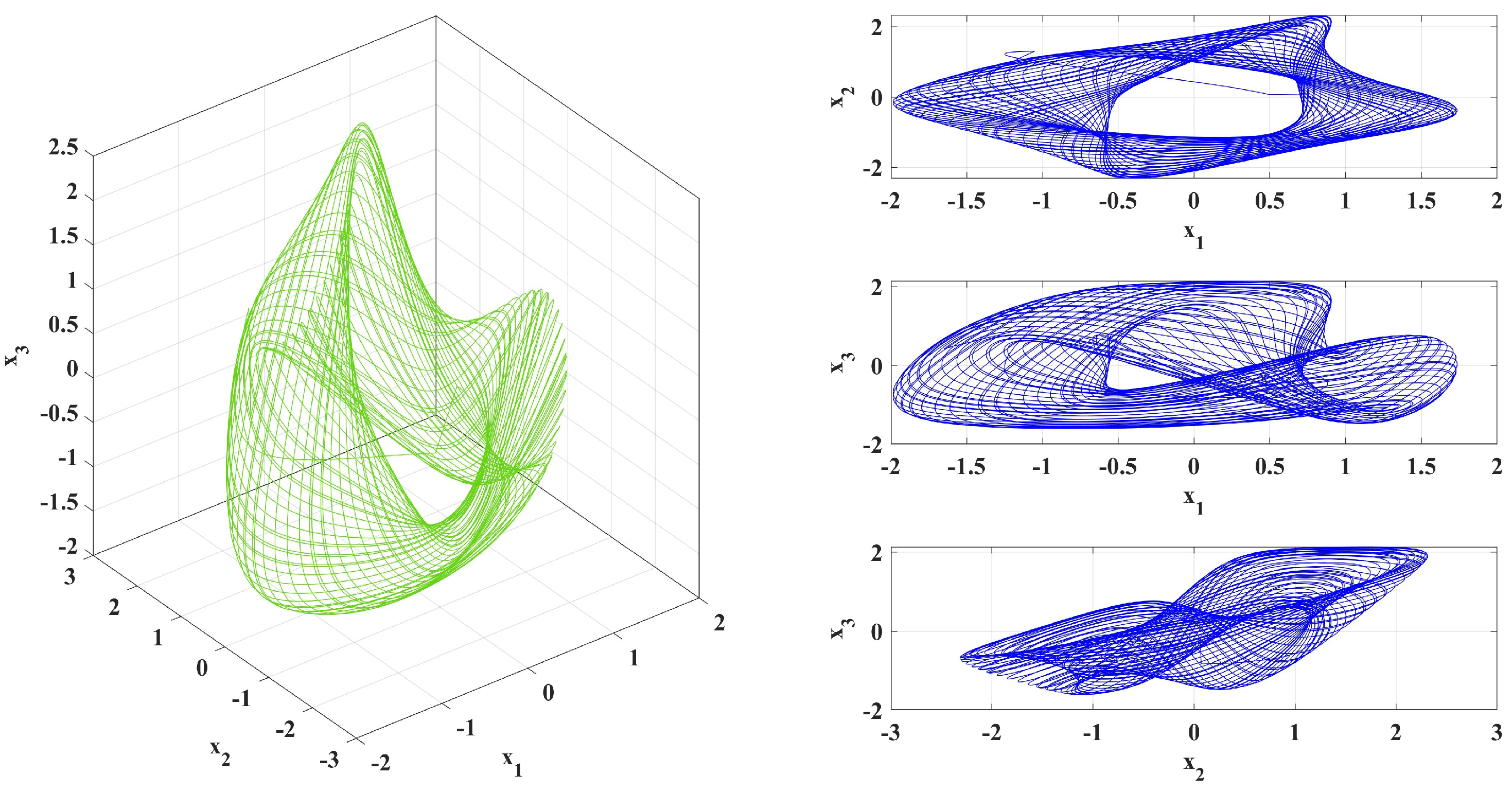
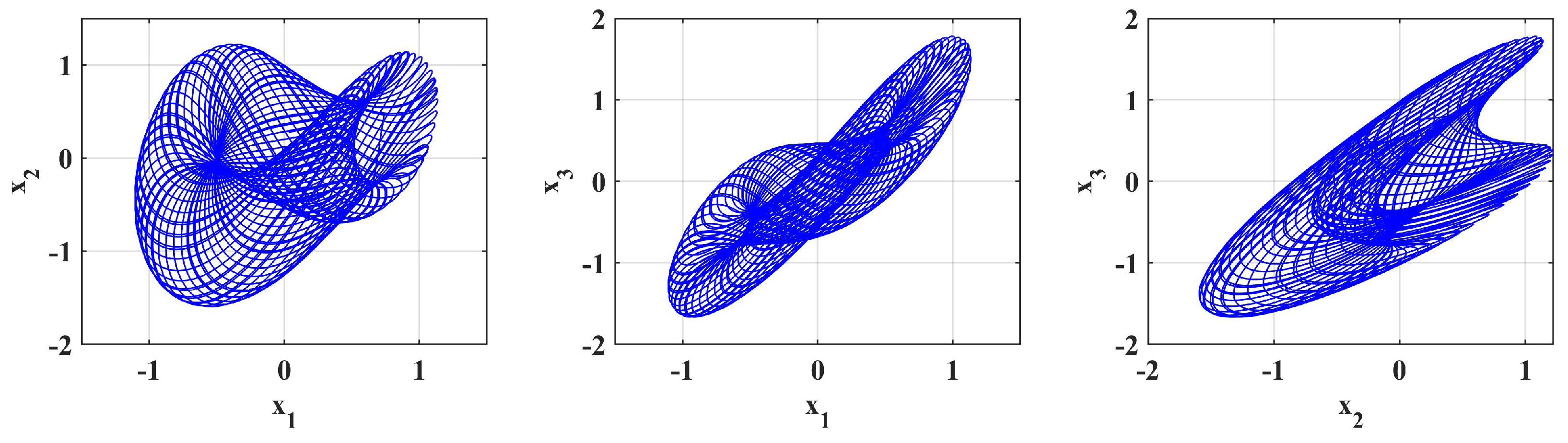
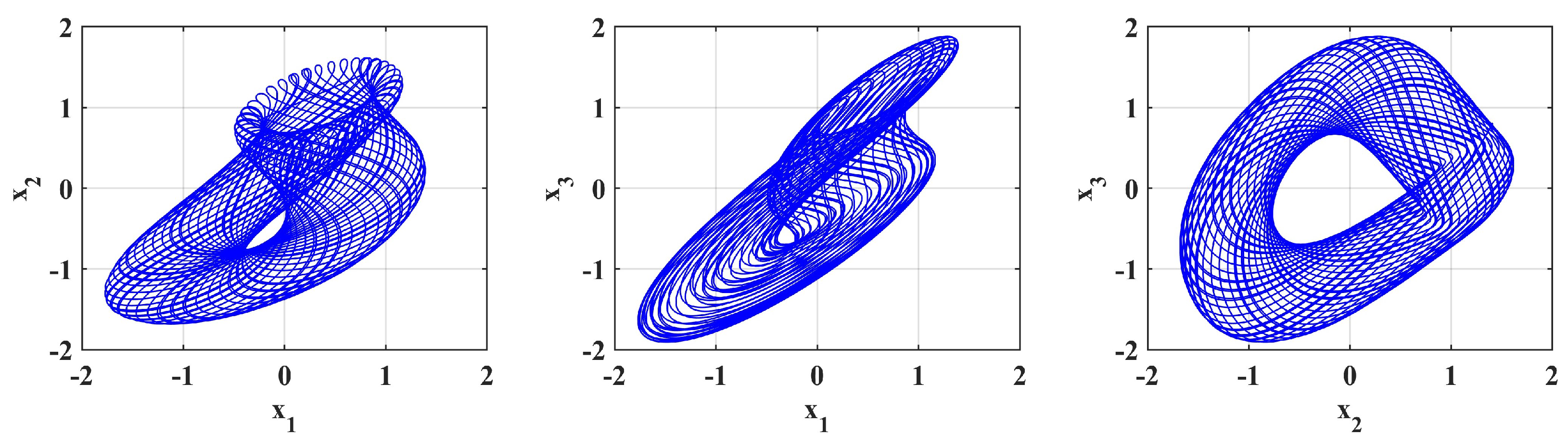
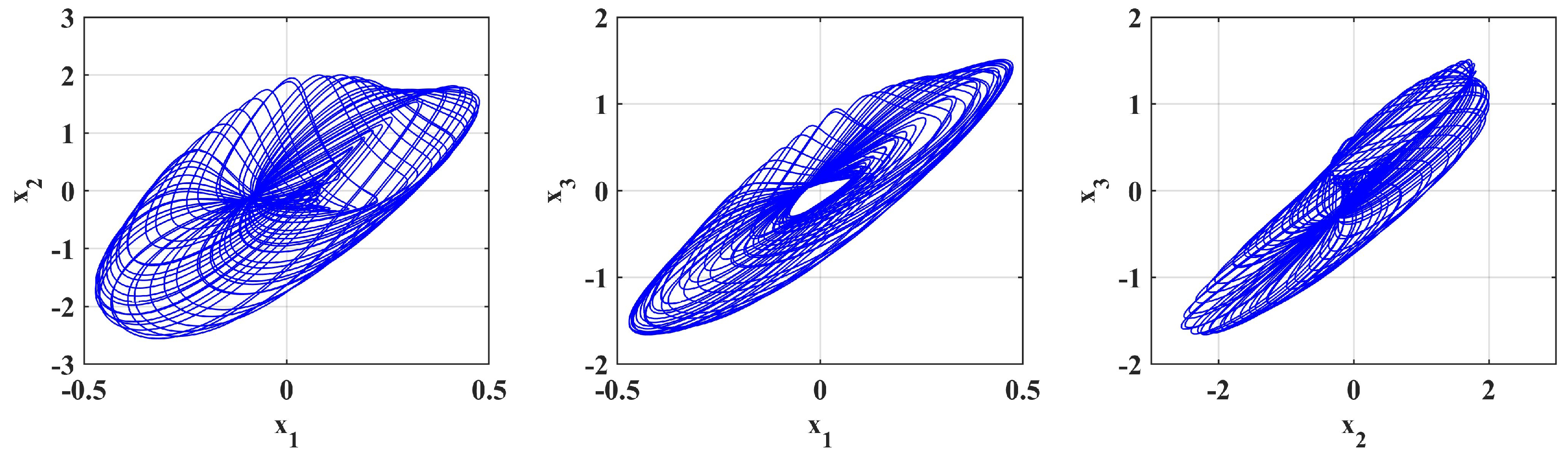
4.1. Phase Portrait of the System

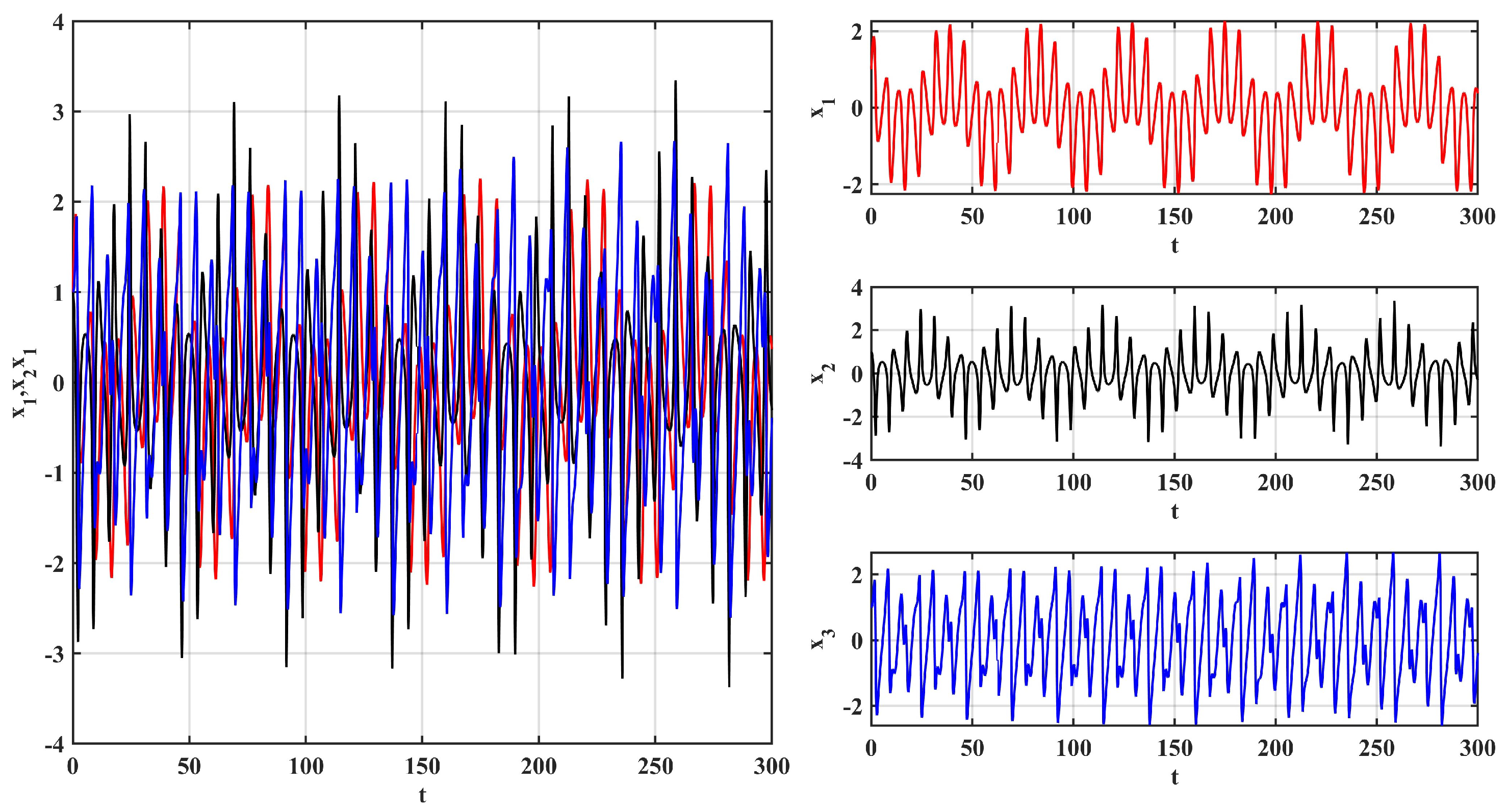
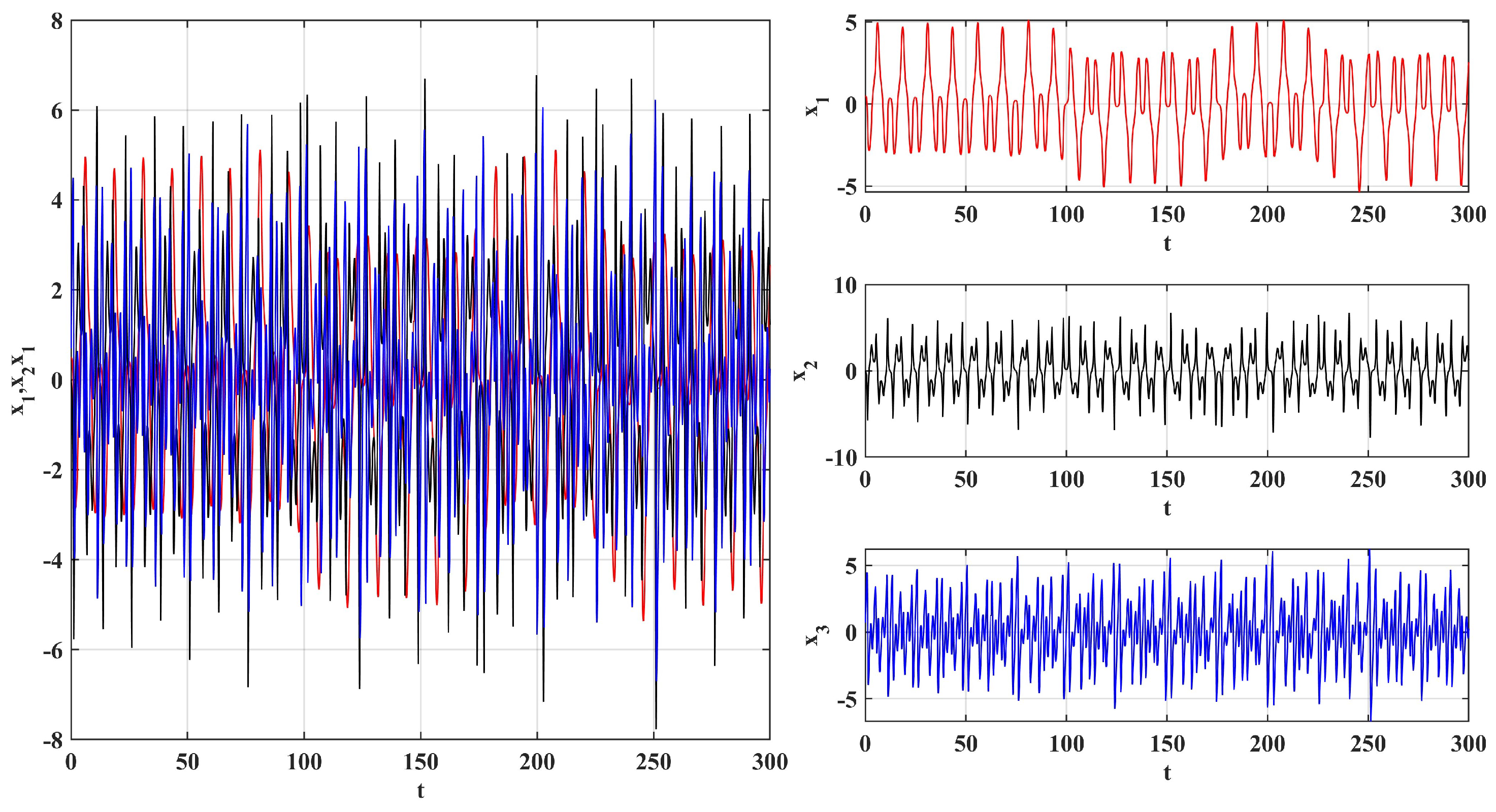
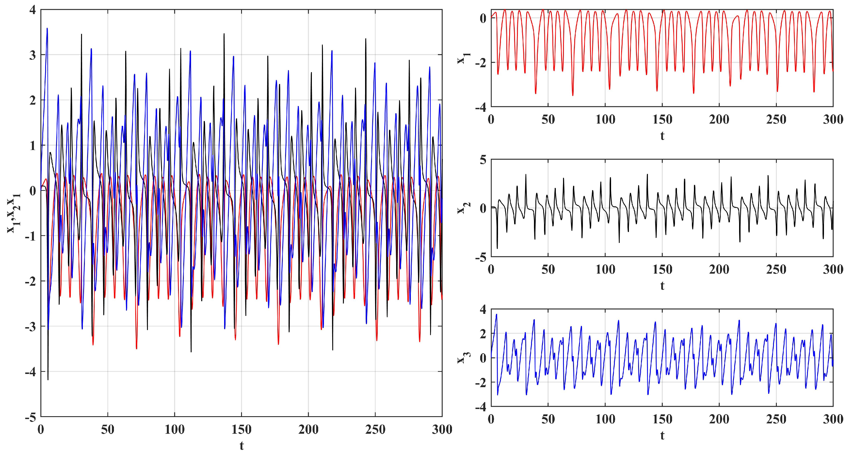
In this part, we show how diverse time-dependent fractional orders $\alpha \left(t\right)$ shape the complex dynamics of a nonlinear system. Figure 1, Figure 2, Figure 3, Figure 4, Figure 5, Figure 6, Figure 7, Figure 8, Figure 9, Figure 10, Figure 11 and Figure 12 illustrate the evolution of attractors of a nonlinear dynamical system for various time-dependent fractional-order functions $\alpha \left(t\right)$. The plots, as 3D phase space trajectories and 2D projections, reveal the sensitivity of the system to the functional shapes of $\alpha$.

Figure 13, Figure 14, Figure 15 and Figure 16 illustrate novel dynamics produced by different time-varying fractional orders $\alpha \left(t\right)$. In Figure 13, ($\alpha =sinh(t/5)+1$), the system is intensely chaotic with expanding spiral structures and pronounced stretching and folding, suggesting increasing memory effects. Figure 14 ($\alpha =1/(3+exp(-2t\left)\right)$) shows a smooth transition to a smooth attractor as $\alpha$ approaches, depicting stabilization with time. As shown in Figure 15 ($\alpha =tanh(t-1)$), the bounded increase of $\alpha$ results in the formation of stable limit cycles after transient divergence—displaying transition from periodicity to chaos. Finally, Figure 16 ($\alpha =1/(2+cos(t/2)$) demonstrates coherent elliptic orbits produced by weak periodic forcing, confirming that infinitesimal oscillations in $\alpha$ regularize the dynamics. These figures reveal the tremendous diversity of behavior generated by altering fractional orders, especially for monotonic, sigmoidal, and periodic variations.

4.2. Time Series

In this part, we analyze the influence of time-varying fractional orders on the temporal behavior of the state variables of the system, as shown in Figure 17, Figure 18 and Figure 19. The time series plots reveal how different functional forms of $\alpha \left(t\right)$ significantly influence the amplitude, frequency, and persistence of oscillations in $x_1$, $x_2$, and $x_3$. For the constant-order case $\alpha =1$ in Figure 17, the system exhibits regular, undamped oscillations, being a stable periodic attractor. Figure 18 shows a new result: for $\alpha =1/(1+exp(-t\left)\right)$.

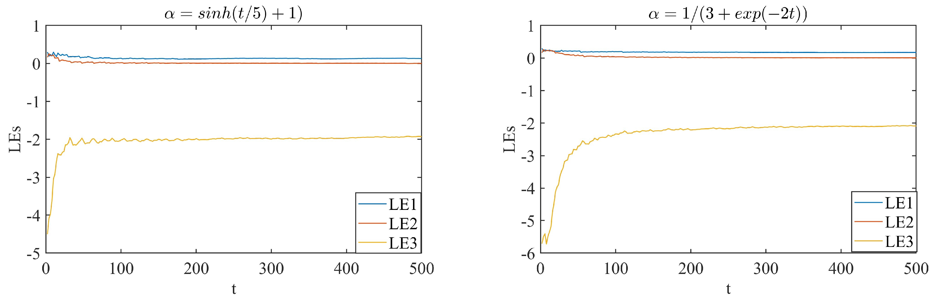
4.3. Lyapunov Exponents

The investigation of chaos in a dynamical system can be systematically established by Lyapunov exponents. They quantify the exponential rate at which initially infinitely close trajectories diverge or converge as time elapses. They provide important insights into the stability of a system and its initial condition sensitivity.

In a dynamical system, the largest Lyapunov exponent, denoted as $\lambda$, plays a crucial role in characterizing the system’s dynamics:

• $\lambda >0$: The system demonstrates sensitivity to initial conditions, indicating chaotic behavior.
• $\lambda =0$: The system displays neutral stability, where trajectories neither show exponential divergence nor convergence.
• $\lambda <0$: Nearby trajectories converge, suggesting that the system is stable and periodic.

The evolution of Lyapunov exponents (LEs) for different orders of variables carries important information on the dynamics of a system. As seen in Figure 20 and Figure 21, the Lyapunov exponents (LE1, LE2, LE3) depend differently on the shape of function $\alpha$. For $\alpha =sinh(t/5)+1$, the exponents rise exponentially, representing increasing chaos, while $\alpha ={\displaystyle \frac{1}{3+exp(-2t)}}$ represents decreasing values from high to low, signifying approaching stability. Similarly, $\alpha =tanh(t-1)$ and $\alpha ={\displaystyle \frac{1}{2+cos(t/2)}}$ introduce oscillatory behavior, with LEs alternating between positive and negative values. This analysis discusses the way that the functional form of $\alpha$ affects the system’s switching from chaotic to stable regimes and enhances the comprehension of underlying complicated dynamics.

5. Numerical Simulation

Figure 1, Figure 2, Figure 3, Figure 4, Figure 5, Figure 6, Figure 7, Figure 8, Figure 9, Figure 10, Figure 11 and Figure 12 collectively demonstrate how the attractors of a nonlinear dynamical system change with various time-dependent parameter functions $\alpha$, as 3D phase space trajectories $(x_1,x_2,x_3)$ and their 2D projections. Figure 1 (the base) establishes a reference point with a butterfly attractor, and Figure 2 ($\alpha =sinh(t/5)+1$) has a hyperbolic sine modification, somewhat changing the loop amplitude. Figure 3 ($\alpha =1/(3+exp(-2t\left)\right)$), Figure 10 ($\alpha =1/(2+exp(-t\left)\right)$), and Figure 11 ($\alpha =1/(4+exp(-6t\left)\right)$) deal with the exponential decay of $\alpha$, analyzing the behavior in shifting from tightly coiled spirals to less restricted loops once the rate of decay decelerates, echoing stability. Figure 4 ($\alpha =tanh(t-1)$) and Figure 5 ($\alpha =1/(2+cos(t/2\left)\right)$) both utilize hyperbolic tangent and cosine functions, resulting in long, oscillatory attractors with skewed projections, characteristic of periodic forcing. Figure 6 ($\alpha =0.90-0.03cosh(t/3)$), Figure 7 ($\alpha =0.07sin(t/7)$), Figure 8 ($\alpha =0.95+0.03exp(t/3)$), Figure 9 ($\alpha =0.90-0.03sinh(t/3)$), and Figure 12 ($\alpha =0.97-0.07sin(t+5)$) further alter $\alpha$ with hyperbolic, sinusoidal, and exponential functions, creating diverse shapes of attractors from tightly wound loops to expanding or non-symmetric patterns.

Figure 17, Figure 18 and Figure 19 show time series plots of a dynamical system whose state variables are $x_1$, $x_2$, and $x_3$ over a time interval $t\in [0,300]$ under different parameter conditions of $\alpha$. That is, Figure 17 has $\alpha =1$, Figure 18 has $\alpha =1/(1+exp(-t\left)\right)$, and Figure 19 has $\alpha =1/(1+exp(t\left)\right)$. Each figure has three subplots: concatenated $x_1,x_2,x_3$ time series on the left (blue for $x_1$, red for $x_2$, and black for $x_3$), and individual plots of $x_3$, $x_1$, and $x_2$ on the right. The figures illustrate the oscillatory nature of the system and how the parameter $\alpha$ affects the amplitude, frequency, and stability of the oscillations. In Figure 11 ($\alpha =1$), the system oscillates regularly with very stable amplitudes in which $x_1$ ranges from approximately $-3$ to 3, $x_2$ ranges from $-4$ to 4, and $x_3$ ranges from $-2$ to 2, showing a periodic attractor with minimal or no damping or growth. Figure 12 ($\alpha =1/(1+exp(-t\left)\right)$) shows an $\alpha$ that varies over time, starting near 0 and increasing to 1 as t grows large (since $exp(-t)\to 0$). This leads to a rise in the oscillation amplitude over time; $x_1$ elongates from $-4$ to 4, $x_2$ elongates from $-5$ to 5, and $x_3$ elongates from $-3$ to 3, indicating the change from damping to larger periodicity as $\alpha$ settles. Conversely, Figure 17 ($\alpha =1/(1+exp(t\left)\right)$) has an $\alpha$ starting near 1 and decaying to 0 as t increases (since $exp\left(t\right)\to \infty$), resulting in a damping effect; the amplitudes of $x_1$, $x_2$, and $x_3$ initially mirror Figure 11 but gradually decrease, with $x_1$ reducing from $-2$ to 2, $x_2$ reducing from $-3$ to 3, and $x_3$ reducing from $-1$ to 1 by $t=300$, reflecting a stabilization or decay of the oscillations. All of these numbers illustrate the sensitivity of the system to $\alpha$. A fixed $\alpha =1$ maintains steady oscillations, an increasing $\alpha$ enlarges them, and a decreasing $\alpha$ damps them, being potentially applicable to modeling such phenomena as mechanical vibrations, neural activity, or ecological cycles in which external parameters influence oscillatory behavior.

Figure 3 ($\alpha =1/(3+exp(-2t\left)\right)$), Figure 6 ($\alpha =0.90-0.03cosh(t/3)$), Figure 10 ($\alpha =1/(2+exp(-t\left)\right)$), Figure 11 ($\alpha =1/(4+exp(-6t\left)\right)$), and Figure 12 ($\alpha =0.97-0.07sin(t+5)$) show phase space trajectories of a dynamical system in 3D and 2D projections. Figure 3 illustrates a close, spiral-shaped attractor as a result of the exponential decay in $\alpha$, progressing towards broader loops in Figure 8 and Figure 11 with variations in the decay rate. Figure 4 illustrates an oscillatory attractor that is influenced by the hyperbolic cosine, and Figure 12 illustrates an asymmetric pattern that arises from the sinusoidal $\alpha$, exhibiting the system’s sensitivity to periodic forcing. The 2D projections present various loop forms, indicating complex periodic behaviors that are adequate for the observation of stability or bifurcations in nonlinear dynamics.

The plots are unique because they show how time-dependent parameter functions $\alpha$ affect the system’s attractors and oscillation behavior in a nonlinear way. The plots represent shifts between stable, damped, and oscillatory regimes, and they reflect the system’s sensitivity to varying $\alpha$ values. Using exponential, hyperbolic, and sinusoidal perturbations, they show how the attractors change from spirals that are coiled up tightly to loops that are pulled out thin. The images convey a richer dynamic.

The selection of variable-order functions is based on their ability to capture diverse memory effects and dynamical behaviors in fractional-order chaotic systems, such as smooth hyperbolic functions ($sinh,cosh,tanh$), exponential functions (exp), periodic trigonometric functions ($sin,cos$), and logistic functions of the form ${\displaystyle \frac{1}{a+exp(-bt)}}$. These functions enable us to analyze how different fractional-order variations influence system stability, chaotic behavior, and attractor evolution. Hyperbolic and exponential functions provide gradual and nonlinear changes in the memory effect, being useful for modeling progressive transitions in system dynamics. On the other hand, trigonometric functions introduce periodic fluctuations, capturing oscillatory memory influences. Logistic-type functions describe sigmoidal transitions, which are relevant in systems where the fractional order changes from one stable state to another. Each function was carefully chosen to ensure numerical stability and to reflect different real-world scenarios in fractional chaotic systems.

Figure 13, $\alpha =sinh(t/5)+1$, shows a system that is chaotic with intense stretching and folding. As $\alpha$ monotonically increases without a bound, trajectories form, expanding spiral patterns with characteristic figure-eight structures in all three projections, indicating strong sensitivity to initial conditions. Figure 14, $\alpha =1/(3+exp(-2t\left)\right)$, shows how these orbits depict more limited dynamics because $\alpha \left(t\right)$ converges slowly toward $1/3$. The system settles to a stable attractor with a smoother orbital structure as opposed to Figure 13, which reflects the asymptotic convergence of the parameter function. Figure 15, $\alpha =tanh(t-1)$, shows how, with the increase in $\alpha$ from a negative to a positive value, the system produces trajectories that first move apart and then stabilize to steady limit cycles. The parameter’s boundedness (tanh saturating at $\pm 1$) ensures that the system remains in some intermediate regime between order and chaos. Figure 16, $\alpha =1/(2+cos(t/2\left)\right)$, shows how the above periodically forced model generates most of the periodic dynamics, in which the orbits take elliptic orbits. Variability of the parameter in the interval $\alpha$ produces coherent and stable orbits in all three projections, showcasing the stabilization of ordered dynamics due to weak periodic forcing.

6. Numerical Solutions

In this part, we analyze the variable-order dynamics of a system through

Table 1. Variable-order values for different state variables with $\alpha =tanh(t+3)$.

t	${\mathit{x}}_1$	${\mathit{x}}_2$	${\mathit{x}}_3$
0.1	0.160618369311393	0.983999926989801	0.002324696443139
0.2	0.271271913153119	0.954369221336363	0.011443865830139
0.3	0.362212867141758	0.918908471316148	0.027225924704286
0.4	0.442152773808205	0.879371780280785	0.049515965151088
0.5	0.514540768830809	0.836527856150666	0.078274324053713
0.6	0.581018359884543	0.790801895468594	0.113511568066676
0.7	0.642399935904049	0.742462013806616	0.155237562733242

,

Table 2. Variable-order values for different state variables with $\alpha =1./(2+exp(-t\left)\right)$.

t	${\mathit{x}}_1$	${\mathit{x}}_2$	${\mathit{x}}_3$
0.1	0.319679618427423	0.920719063255373	0.035343702874417
0.2	0.422676269071848	0.862630499078330	0.083581018263259
0.3	0.490850043028715	0.815895079674831	0.133293059665953
0.4	0.542646170337882	0.775920823500659	0.182911887184131
0.5	0.584928279692839	0.740249450751355	0.232307866573166
0.6	0.621015049995438	0.707399030963379	0.281700335765962
0.7	0.652737697455643	0.676399787022939	0.331386860115778

and

Table 3. Variable-order values for different state variables with $\alpha =0.95-0.05·cos(t/5)$.

t	${\mathit{x}}_1$	${\mathit{x}}_2$	${\mathit{x}}_3$
0.1	0.129253322964099	0.990770704789030	0.000924568232129
0.2	0.240126615822257	0.968031069379841	0.005992097825715
0.3	0.341787791177007	0.934858280605783	0.017554947037803
0.4	0.435525899311576	0.893351536370992	0.037089876307740
0.5	0.521666320880403	0.845277281367284	0.065412627621342
0.6	0.600295728515390	0.792120482521920	0.102813647581629
0.7	0.671446014982371	0.735077009819927	0.149182051061457

, which hold the values of $x_1$, $x_2$, and $x_3$ for different $\alpha$ functions over $t\in [0.1,0.7]$, along with phase space trajectories in Figure 3, Figure 6 and Figure 10, Figure 11 and Figure 12. Table 1 ($V_x=tanh(t+3)$) shows $V_{x_1}$ rising from 0.1606 to 0.6424, $V_{x_2}$ falling from 0.9840 to 0.7425, and $V_{x_3}$ rising from 0.0023 to 0.1552, suggesting an increase in higher-order dynamics in $x_3$. Table 2 ($\alpha =1/(2+exp(-t\left)\right)$) shows the same trend, with $x_1$ increasing from 0.3197 to 0.6527, $x_2$ increasing from 0.9207 to 0.6764, and $x_3$ increasing from 0.0353 to 0.3314, having a more extreme effect on $x_3$ with the exponential decline in $\alpha$. Table 3 ($\alpha =0.95-0.05cos(t/5)$) shows $x_1$ rising from 0.1293 to 0.6714, $x_2$ falling from 0.9908 to 0.7351, and $x_3$ rising from 0.0009 to 0.1492, illustrating oscillatory modulation in the dynamics. Likewise, Figure 3 ($\alpha =1/(3+exp(-2t\left)\right)$) and Figure 10 and Figure 11 ($\alpha =1/(2+exp(-t\left)\right)$ and $\alpha =1/(4+exp(-6t\left)\right)$) demonstrate compact to broad spiral attractors, reflecting the exponential decay’s stabilizing effect, while Figure 6 ($\alpha =0.90-0.03cosh(t/3)$) and Figure 10 ($\alpha =0.97-0.07sin(t+5)$) show oscillatory and asymmetric patterns, respectively, reflecting the variable-order trends and highlighting the system’s sensitivity to $\alpha$ temporal variations.

7. Conclusions

This study of novel variable-order fractional chaotic systems confirms their temporal versatility through numerical simulations and solutions. The phase space traces in the figures, guided by different $\alpha$ functions $\alpha$, show a wide range of shapes for the attractor—compact spirals and stretched patterns—underscoring the susceptibility of the system to the temporal variations of $\alpha$. The time series plots of the figures also indicate how $\alpha$ affects the oscillation amplitude and stability, with larger $\alpha$ values increasing oscillations and smaller $\alpha$ values causing damping. Furthermore, the tables demonstrate the development of variable-order parameters $x_1$, $x_2$, and $x_3$, with a noticeable increase in $x_3$, which emphasizes the increase in chaotic behavior. These outcomes demonstrate the capability of variable-order derivatives regarding the rich expression of dynamics with good engineering and physical applicability. The efficient optimization of these variable-order parameters in an ensuing work would further enhance their physical and engineering utility.

References

1. Alsubaie, N.E.; EL Guma, F.; Boulehmi, K.; Al-kuleab, N.; Abdoon, M.A. Improving influenza epidemiological models under Caputo fractional-order calculus. Symmetry 2024, 16, 929. [Google Scholar] [CrossRef]
2. Alharbi, S.A.; Abdoon, M.A.; Degoot, A.M.; Alsemiry, R.D.; Allogmany, R.; ELGuma, F.; Berir, M. Mathematical modeling of influenza dynamics: A novel approach with SVEIHR and fractional calculus. Int. J. Biomath. 2025, 2025, 2450147. [Google Scholar] [CrossRef]
3. Abdoon, M.A.; Alzahrani, A.B.M. Comparative analysis of influenza modeling using novel fractional operators with real data. Symmetry 2024, 16, 1126. [Google Scholar] [CrossRef]
4. Abdoon, M.A.; Elgezouli, D.E.; Halouani, B.; Abdelaty, A.M.Y.; Elshazly, I.S.; Ailawalia, P.; El-Qadeem, A.H. Novel dynamic behaviors in fractional chaotic systems: Numerical simulations with Caputo derivatives. Axioms 2024, 13, 791. [Google Scholar] [CrossRef]
5. Tarasov, V.E.; Zaslavsky, G.M. Fractional dynamics of systems with long-range space interaction and temporal memory. Phys. A Stat. Mech. Appl. 2007, 383, 291–308. [Google Scholar] [CrossRef]
6. Picozzi, S.; West, B.J. Fractional Langevin model of memory in financial markets. Phys. Rev. E 2002, 66, 046118. [Google Scholar] [CrossRef]
7. Daoui, A.; Yamni, M.; Karmouni, H.; Sayyouri, M.; Qjidaa, H.; Ahmad, M.; Abd El-Latif, A.A. Biomedical multimedia encryption by fractional-order Meixner polynomials map and quaternion fractional-order Meixner moments. IEEE Access 2022, 10, 102599–102617. [Google Scholar] [CrossRef]
8. Bhatnagar, G.; Wu, Q.M.J.; Raman, B. Discrete fractional wavelet transform and its application to multiple encryption. Inf. Sci. 2013, 223, 297–316. [Google Scholar] [CrossRef]
9. Kiani-B., A.; Fallahi, K.; Pariz, N.; Leung, H. A chaotic secure communication scheme using fractional chaotic systems based on an extended fractional Kalman filter. Commun. Nonlinear Sci. Numer. Simul. 2009, 14, 863–879. [Google Scholar] [CrossRef]
10. Rahman, Z.-A.S.A.; Jasim, B.H.; Al-Yasir, Y.I.A.; Hu, Y.-F.; Abd-Alhameed, R.A.; Alhasnawi, B.N. A new fractional-order chaotic system with its analysis, synchronization, and circuit realization for secure communication applications. Mathematics 2021, 9, 2593. [Google Scholar] [CrossRef]
11. Alqahtani, F.; Amoon, M.; El-Shafai, W. A fractional Fourier based medical image authentication approach. CMC-Comput. Mater. Contin. 2022, 70, 3133–3150. [Google Scholar] [CrossRef]
12. Denis, R.; Madhubala, P. Hybrid data encryption model integrating multi-objective adaptive genetic algorithm for secure medical data communication over cloud-based healthcare systems. Multimed. Tools Appl. 2021, 80, 21165–21202. [Google Scholar] [CrossRef]
13. Martínez-Guerra, R.; Pérez-Pinacho, C.A. Advances in Synchronization of Coupled Fractional Order Systems: Fundamentals and Methods; Springer: Cham, Switzerland, 2018. [Google Scholar]
14. Martínez-Guerra, R.; Gómez-Cortés, G.C.; Pérez-Pinacho, C.A. Synchronization of integral and fractional order chaotic systems. In A Differential Algebraic and Differential Geometric Approach; Springer: Cham, Switzerland, 2015. [Google Scholar]
15. Luo, C.; Wang, X. Chaos in the fractional-order complex Lorenz system and its synchronization. Nonlinear Dyn. 2013, 71, 241–257. [Google Scholar] [CrossRef]
16. Sheng, H.; Chen, Y.Q.; Qiu, T. Fractional Processes and Fractional-Order Signal Processing: Techniques and Applications; Springer Science & Business Media: London, UK, 2011. [Google Scholar]
17. Tepljakov, A. Fractional-Order Modeling and Control of Dynamic Systems; Springer: Cham, Switzerland, 2017. [Google Scholar]
18. Beyene, G.A.; Rahma, F.; Rajagopal, K.; Al-Hussein, A.-B.A.; Boulaaras, S. Dynamical analysis of a 3D fractional-order chaotic system for high-security communication and its electronic circuit implementation. J. Nonlinear Math. Phys. 2023, 30, 1375–1391. [Google Scholar] [CrossRef]
19. Iqbal, S.; Wang, J. A novel fractional-order 3-D chaotic system and its application to secure communication based on chaos synchronization. Phys. Scr. 2025, 100, 025243. [Google Scholar] [CrossRef]
20. Zhang, J.-X.; Zhang, X.; Boutat, D.; Liu, D.-Y. Fractional-Order Complex Systems: Advanced Control, Intelligent Estimation and Reinforcement Learning Image-Processing Algorithms. Fractal Fract. 2025, 9, 67. [Google Scholar] [CrossRef]
21. Patnaik, S.; Hollkamp, J.P.; Semperlotti, F. Applications of variable-order fractional operators: A review. Proc. R. Soc. A 2020, 476, 20190498. [Google Scholar] [CrossRef]
22. Vellappandi, M.; Lee, S. Neural fractional differential networks for modeling complex dynamical systems. Nonlinear Dyn. 2024, 113, 12117–12130. [Google Scholar] [CrossRef]
23. Erdinc, U.; Bilgil, H.; Ozturk, Z. A novel fractional forecasting model for time dependent real world cases. REVSTAT-Stat. J. 2024, 22, 169–188. [Google Scholar]
24. Sprott, J.C. Some simple chaotic flows. Phys. Rev. E 1994, 50, R647. [Google Scholar] [CrossRef]
25. Mekkaoui, T.; Hammouch, Z.; Belgacem, F.; El Abbassi, A. Fractional-order nonlinear systems: Chaotic dynamics, numerical simulation and circuits design. In Fractional Dynamics; De Gruyter Brill: Berlin, Germany, 2015; pp. 343–356. [Google Scholar]
26. Khan, M.A.; Atangana, A.; Muhammad, T.; Alzahrani, E. Numerical solution of a fractal-fractional order chaotic circuit system. Rev. Mex. FíSica 2021, 67, 051401. [Google Scholar]
27. Podlubny, I. Fractional Differential Equations: An Introduction to Fractional Derivatives, Fractional Differential Equations, to Methods of Their Solution and Some of Their Applications; Elsevier: Amsterdam, The Netherlands, 1998. [Google Scholar]
28. Solís-Pérez, J.E.; Gómez-Aguilar, J.F.; Atangana, A. Novel numerical method for solving variable-order fractional differential equations with power, exponential and Mittag-Leffler laws. Chaos Solitons Fractals 2018, 114, 175–185. [Google Scholar] [CrossRef]
29. Kshirsagar, K.; Nikam, V.; Gaikwad, S.; Tarate, S. Fuzzy Laplace-Adomian Decomposition Method for Solving Fuzzy Klein-Gordan Equations. Q. J. R. Meteorol. Soc. 2017, 1–6. [Google Scholar] [CrossRef]
30. Bildik, N. Implementation to the Different Differential Equations of Homotopy Analysis, Differential Transformed and Adomian Decomposition Method. Int. J. Model. Optim. 2013, 3, 529–534. [Google Scholar] [CrossRef]
31. Baskonus, H.M.; Bulut, H. On the numerical solutions of some fractional ordinary differential equations by fractional Adams-Bashforth-Moulton method. Open Math. 2015, 13, 000010151520150052. [Google Scholar] [CrossRef]
32. Pu, Y.-F. Fractional-order Euler-Lagrange equation for fractional-order variational method: A necessary condition for fractional-order fixed boundary optimization problems in signal processing and image processing. IEEE Access 2016, 4, 10110–10135. [Google Scholar] [CrossRef]
33. Ramalakshmi, K.; Sundaravadivoo, B. Necessary conditions for Ψ-Hilfer fractional optimal control problems and Ψ-Hilfer two-step Lagrange interpolation polynomial. Int. J. Dyn. Control 2024, 12, 42–55. [Google Scholar] [CrossRef]
34. Buhader, A.A.; Abbas, M.; Imran, M.; Omame, A. Comparative analysis of a fractional co-infection model using nonstandard finite difference and two-step Lagrange polynomial methods. Partial Differ. Equ. Appl. Math. 2024, 10, 100702. [Google Scholar] [CrossRef]
35. Alqahtani, A.M.; Chaudhary, A.; Dubey, R.S.; Sharma, S. Comparative analysis of the chaotic behavior of a five-dimensional fractional hyperchaotic system with constant and variable order. Fractal Fract. 2024, 8, 421. [Google Scholar] [CrossRef]
36. Butt, A.I.K.; Ahmad, W.; Rafiq, M.; Baleanu, D. Numerical analysis of Atangana-Baleanu fractional model to understand the propagation of a novel corona virus pandemic. Alex. Eng. J. 2022, 61, 7007–7027. [Google Scholar] [CrossRef]
37. Elbadri, M.; Abdoon, M.A.; Alzahrani, A.B.M.; Saadeh, R.; Berir, M. A comparative study and numerical solutions for the fractional modified Lorenz–Stenflo system using two methods. Axioms 2024, 14, 20. [Google Scholar] [CrossRef]
38. Cafagna, D.; Grassi, G. Chaos in a new fractional-order system without equilibrium points. Commun. Nonlinear Sci. Numer. Simul. 2014, 19, 2919–2927. [Google Scholar] [CrossRef]
39. Pham, V.-T.; Volos, C.; Jafari, S.; Wang, X.; Vaidyanathan, S. Hidden Hyperchaotic Attractor in a Novel Simple Memristive Neural Network. Optoelectronics Adv. Mater. Commun. 2014, 8, 1157–1163. [Google Scholar]
40. Hartley, T.T.; Lorenzo, C.F.; Qammer, H.K. Chaos in a fractional order Chua’s system. IEEE Trans. Circuits Syst. I Fundam. Theory Appl. 1995, 42, 485–490. [Google Scholar] [CrossRef]
41. Lu, J.-G. Chaotic dynamics and synchronization of fractional-order Genesio–Tesi systems. Chin. Phys. 2005, 14, 1517. [Google Scholar]
Figure 1. Visualization of system trajectories for the original α .
Fractalfract 09 00277 g001
Figure 2. Visualization of system trajectories for α = ( s i n h ( t / 5 ) + 1 ) .
Fractalfract 09 00277 g002
Figure 3. Visualization of system trajectories for α = 1 / ( 3 + e x p ( 2 t ) ) .
Fractalfract 09 00277 g003
Figure 4. Visualization of system trajectories for α = t a n h ( t 1 ) .
Fractalfract 09 00277 g004
Figure 5. Visualization of system trajectories for α = 1 / 2 + ( c o s ( t / 2 ) ) .
Fractalfract 09 00277 g005
Figure 6. Visualization of system trajectories for α = 0.90 0.03 ( c o s h ( t / 3 ) ) .
Fractalfract 09 00277 g006
Figure 7. Visualization of system trajectories for α = 0.07 ( s i n ( t / 7 ) ) .
Fractalfract 09 00277 g007
Figure 8. Visualization of system trajectories for α = 0.95 + 0.03 ( e x p ( t / 3 ) ) .
Fractalfract 09 00277 g008
Figure 9. Visualization of system trajectories for α = 0.90 0.03 ( s i n h ( t / 3 ) ) .
Fractalfract 09 00277 g009
Figure 10. Visualization of system trajectories for α = 1 / ( 2 + e x p ( t ) ) .
Fractalfract 09 00277 g010
Figure 11. Visualization of system trajectories for α = 1 / ( 4 + e x p ( 6 t ) ) .
Fractalfract 09 00277 g011
Figure 12. Visualization of system trajectories for α = 0.97 0.07 ( s i n ( t + 5 ) ) .
Fractalfract 09 00277 g012
Figure 13. Visualization of system trajectories for ( α = sinh ( t / 5 ) + 1 ).
Fractalfract 09 00277 g013
Figure 14. Visualization of system trajectories for ( α = 1 / ( 3 + exp ( 2 t ) ) ).
Fractalfract 09 00277 g014
Figure 15. Visualization of system trajectories for ( α = tanh ( t 1 ) ).
Fractalfract 09 00277 g015
Figure 16. Visualization of system trajectories for ( α = 1 / ( 2 + cos ( t / 2 ) ) ).
Fractalfract 09 00277 g016
Figure 17. Oscillatory dynamics of a system with α = 1 .
Fractalfract 09 00277 g017
Figure 18. Oscillatory dynamics of a system with α = 1 / ( 1 + e x p ( t ) ) .
Fractalfract 09 00277 g018
Figure 19. Oscillatory dynamics of a system with α = 1 / t a n h ( t 1 ) .
Fractalfract 09 00277 g019
Figure 20. Evolution of Lyapunov exponents for different variable orders.
Fractalfract 09 00277 g020
Figure 21. Evolution of Lyapunov exponents for different variable orders.
Fractalfract 09 00277 g021