Linear and Non-Linear Methods to Discriminate Cortical Parcels Based on Neurodynamics: Insights from sEEG Recordings

Abstract

Understanding human cortical neurodynamics is increasingly important, as highlighted by the European Innovation Council, which prioritises tools for measuring and stimulating brain activity. Unravelling how cytoarchitecture, morphology, and connectivity shape neurodynamics is essential for developing technologies that target specific brain regions. Given the dynamic and non-stationary nature of neural interactions, there is an urgent need for non-linear signal analysis methods, in addition to the linear ones, to track local neurodynamics and differentiate cortical parcels. Here, we explore linear and non-linear methods using data from a public stereotactic intracranial EEG (sEEG) dataset, focusing on the superior temporal gyrus (STG), postcentral gyrus (postCG), and precentral gyrus (preCG) in 55 subjects during resting-state wakefulness. For this study, we used a linear Power Spectral Density (PSD) estimate and three non-linear measures: the Higuchi fractal dimension (HFD), a one-dimensional convolutional neural network (1D-CNN), and a one-shot learning model. The PSD was able to distinguish the regions in α, β, and γ frequency bands. The HFD showed a tendency of a higher value in the preCG than in the postCG, and both were higher in the STG. The 1D-CNN showed promise in identifying cortical parcels, with an 85% accuracy for the training set, although performance in the test phase indicates that further refinement is needed to integrate dynamic neural electrical activity patterns into neural networks for suitable classification.

1. Introduction

Neuronal electrical activity (neurodynamics) at rest is an expression of the interaction of many neurons acting together [1]. Such activity in the brain can be measured through electroencephalography (EEG), magnetoencephalography (MEG), or stereotactical-intracranial electroencephalography (sEEG) recordings [2]. All three measures provide an optimal temporal resolution for the observation of neural dynamics. However, the latter provides a direct measurement of neuronal pool activity, avoiding the attenuation of the signal that occurs when it passes through the brain tissues to electrodes on the surface of the scalp. The obtained neural signals are chaotic, thus requiring various measures that could help in finding the characteristic features in them [3]. One of the traditional methods for such analysis is the Power Spectral Density (PSD) method, where the power in different frequency bands is observed [4]. On the other hand, it is a linear estimate, and in addition to neurophysiological signals, most of the time, it contains non-stationarity and complexity [5]. Thus, here, deploying fractality measures are needed, such as the Higuchi fractal dimension (HFD) [6]. This is a method used to analyse the complexity of natural time series [7,8,9]. Unlike traditional linear measures, the HFD captures how self-similar and irregular brain activity is over time, providing insights into neural dynamics [10]. This is particularly useful in studying brain function and detecting abnormalities in conditions like epilepsy or neurodegenerative diseases [6].

Analysing neurophysiological signals is essential for comprehending the intricate dynamics of brain function and its alterations in various pathological conditions. These conditions arise from disrupted circuitry in certain brain areas due to neurodegenerative processes [11,12] or various genetic factors [13]. The neural activity of different brain regions is strongly related to the anatomical connectivity of neural networks and may exhibit different biases in their interactions within brain networks, depending on the pathway of information flow. For example, in the somatosensory cortex, external stimuli interact with the resting state somatosensory brain network, which may result in different functional neural network configurations, depending on the specific stimulus [14]. In the motor cortex, it is capable of retaining information about movements seconds before the actual execution occurs [15]; this may happen due to the planning of the movement. Therefore, at the microscale level and in relation to specific tasks, the differences in neurodynamics between brain areas are relatively well understood. However, while there are studies supporting the neural network connectivity between brain regions constituting the default mode network [16,17], the literature on how this connectivity affects the local neurodynamics of separate brain parcels is rather scarce. Despite this, it is important to understand and characterize local brain neural activity and its generating processes at rest in healthy conditions, as this can enhance our ability to predict deviations from normal activity, such as those occurring in early neurodegenerative processes or other brain disorders, and possibly aid in creating computational models to define these deviations.

Thus, in this study, using sEEG recordings from three cortical parcels—superior temporal gyrus (STG), postcentral gyrus (postCG), and precentral gyrus (preCG)—we aim to investigate whether these different cortical parcels systematically exhibit diverse characteristic neurodynamical activities as measured through linear and non-linear techniques, as well as deep neural networks. The deployment of several methods could permit us to obtain more reliable results and contribute to the research on the best methods in performing such tasks. The importance of such an investigation is in the attempt to parcel the brain regions from neurodynamics instead of cytoarchitecture.

2. Materials and Methods

Our analysis was carried out on sEEG recordings from an open database published by the Montreal Neurological Institute (MNI). The whole dataset consists of a dense coverage sEEG across various brain regions from 106 subjects, suffering from drug-resistant epilepsy, who were investigated before the epileptogenic zone removal surgery. Subjects are proportionally distributed across genders and aged 13–68 years old. All recordings are only from healthy regions, recorded with bipolar channels with a 10 mm diameter. Recordings are 60 s long each, sampled at 200 Hz, with a low-pass filter at 80 Hz, detected at resting wakefulness, with eyes open. Power-line interference is mitigated using an adaptive filtering approach involving a high-pass FIR filter, harmonic phase and amplitude estimation, and the subtraction of estimated interference components in descending harmonic order. The power-line frequency applied depended on the country in which the recordings were collected: 50 Hz for data from France and 60 Hz for data from Canada [4]. Additionally, artifacts were manually identified and excluded by a neurophysiologist. The recordings were obtained using cortical surface grids or strips [4]. In agreement with previous studies, we did not differentiate between the electrode types [4].

We investigated the primary motor and sensory regions, precisely because from the cortical point of view, they are the nodes that receive and send the coordination signals from and to our body; therefore, they are actually the most connected regions, the main hub of our entire brain. Thus, we studied the precentral gyrus, postcentral gyrus, and superior temporal gyrus of the two hemispheres (Figure 1), in agreement with the classification provided by the MNI dataset [4,18]. It is possible to deploy the same analysis procedure for sEEG recordings collected with a different type of electrode [4,18]. Due to the nature of MNI sEEG dataset collected in people affected by epilepsy, the number of channels available for each region is not homogenous.

In total, we analysed 284 channels from total 55 subjects, distributed as follows:

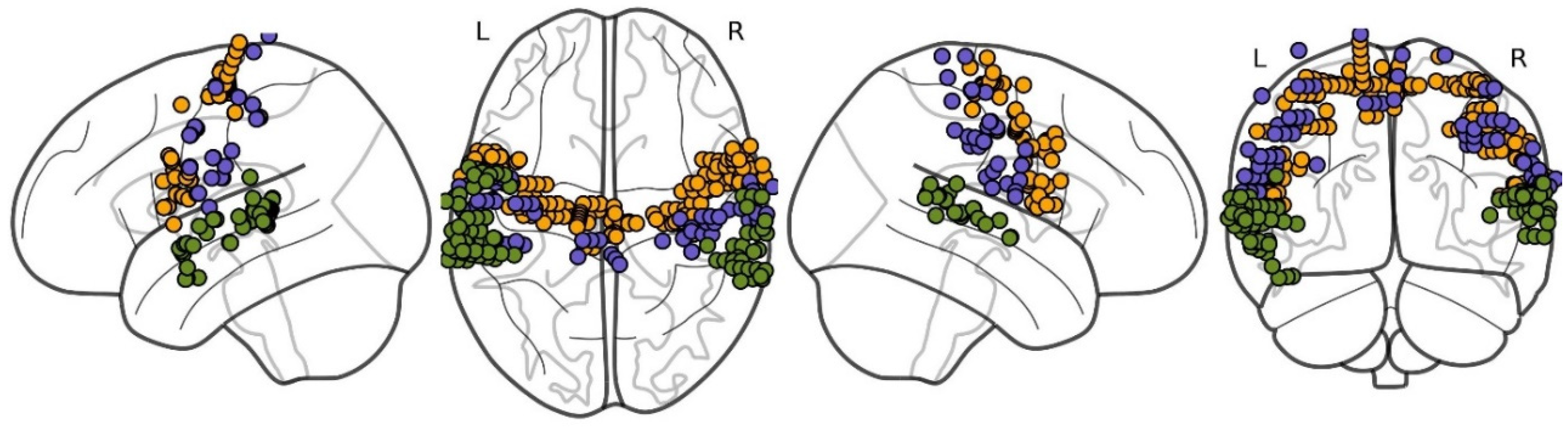
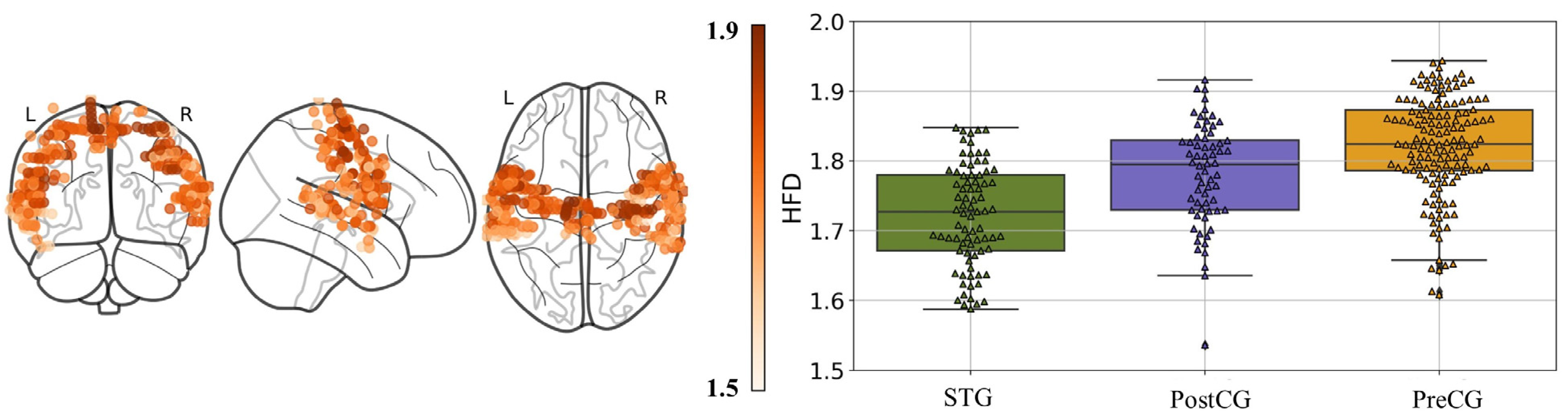
• precentral gyrus (PreCG): 141 channels (from 34 subjects);
• postcentral gyrus (PostCG): 64 channels (from 21 subjects);
• superior temporal gyrus (STG): 79 channels (from 26 subjects).

2.1. Spectral Analysis

In order to investigate the spectral signature of the three cortical areas, we studied the PSD of their sEEG recordings. For each channel of each region, we calculated the Fast Fourier Transform (FFT) on blocks of 256 samples, with the Hamming windowing without overlap, according with the Welch procedure [19], and averaged the resulting periodograms. We divided the spectrum in the traditional five frequency bands as follows: δ ≤ 4 Hz; θ (4–8] Hz; α (8–12] Hz; β (12–33] Hz; and γ (33–80] Hz.

For the comparisons of the spectral differences between the three cortical parcels in a single band, for each region, we averaged the PSD of a channel separately in every frequency band.

2.2. Higuchi Fractal Dimension

In the framework of the literature investigating fractal estimation methods of neurodynamics, we estimated the fractality via the HFD [9]. It has been claimed that the HFD performed best in estimating the fractal properties of EEG signals, and it has been suggested as biomarker in healthy and pathological conditions [5,20,21,22,23]. One of the advantages of Higuchi’s algorithm is that it works directly in the time domain; therefore, it can be evaluated directly in the time series of sEEG. The calculation of the HFD is as follows [9]:

According to the concept of quantifying the emergence of similar features at different time scales, Higuchi’s algorithm uses many time series $X_k^m$, built by down-sampling the original series {X(i)} with i = 1, …, N, for every k sample:

$$X_k^m=\{ X(m), X(m+k), X(m+2k), \dots , X(m+\left(\right(N-m)/k)\left)k\right)\}$$

where k is an integer (1 < k ≤ k_max, with k_max < N/2) and m = 1, 2, 3, …, k.

Then, the length $L_m\left(k\right)$ of the curve $X_k^m$, is defined as the average value over k − 1 sets of $X_m\left(k\right)$ as follows:

$$L_m\left(k\right)=\left[\left(\sum _{i=1}^{int\left({\displaystyle \frac{N-m}{k}}\right)}\left|X\left(m+i k\right)-X\left(m+\left(i-1\right)k\right)\right|\right){\displaystyle \frac{N-1}{int\left(\frac{N-m}{k}\right)k}}\right]{\displaystyle \frac{1}{k}}$$

The length $L\left(k\right)$ is defined as the average of the k lengths $L_m\left(k\right)$: $L\left(k\right)={\displaystyle \frac{1}{k}}\sum _{m=1}^k{L}_m\left(k\right)$. If, for k → k_max, the limit of the ratio ${\displaystyle \frac{log\left(L_m\left(k\right)\right)}{log\left(k\right)}}$ exists, we can write that $L\left(k\right)\approx k^{-HFD}$ and the curve {X(i)} is a fractal with a dimension equal to the HFD. It is worth noting that the estimation of the HFD can depend on the adopted value of k_max, and generally, it is evaluated at the value of k_max to which the HFD (k_max) curve vs. k_max starts reaching a plateau [20,24]. The interpretation of the HFD as an estimation of the “true”/asymptotic fractal dimension of a temporal series has been questioned [25]. However, for a fixed value of k_max, the HFD (k_max) has largely been adopted in the literature [22,26,27,28] as a reliable index of fractality that is able to discriminate between several states, being sensitive to their variation in complexity, mainly as a function of time [29]. We computed the HFD (k_max) at k_max = 35, which we keep fixed across all subjects and the three areas. The selection of k_max = 35 is based on the reasoning that when the HFD value is represented versus the k_max, it follows a curve, which saturates at some point and afterward, starts reaching the asymptote. Thus, for these data, the asymptote was reached at the value of k_max = 35. The method of setting the k_max value is in agreement with the literature [10,20] and has been already published for this specific dataset [24].

2.3. Deep Learning Classification

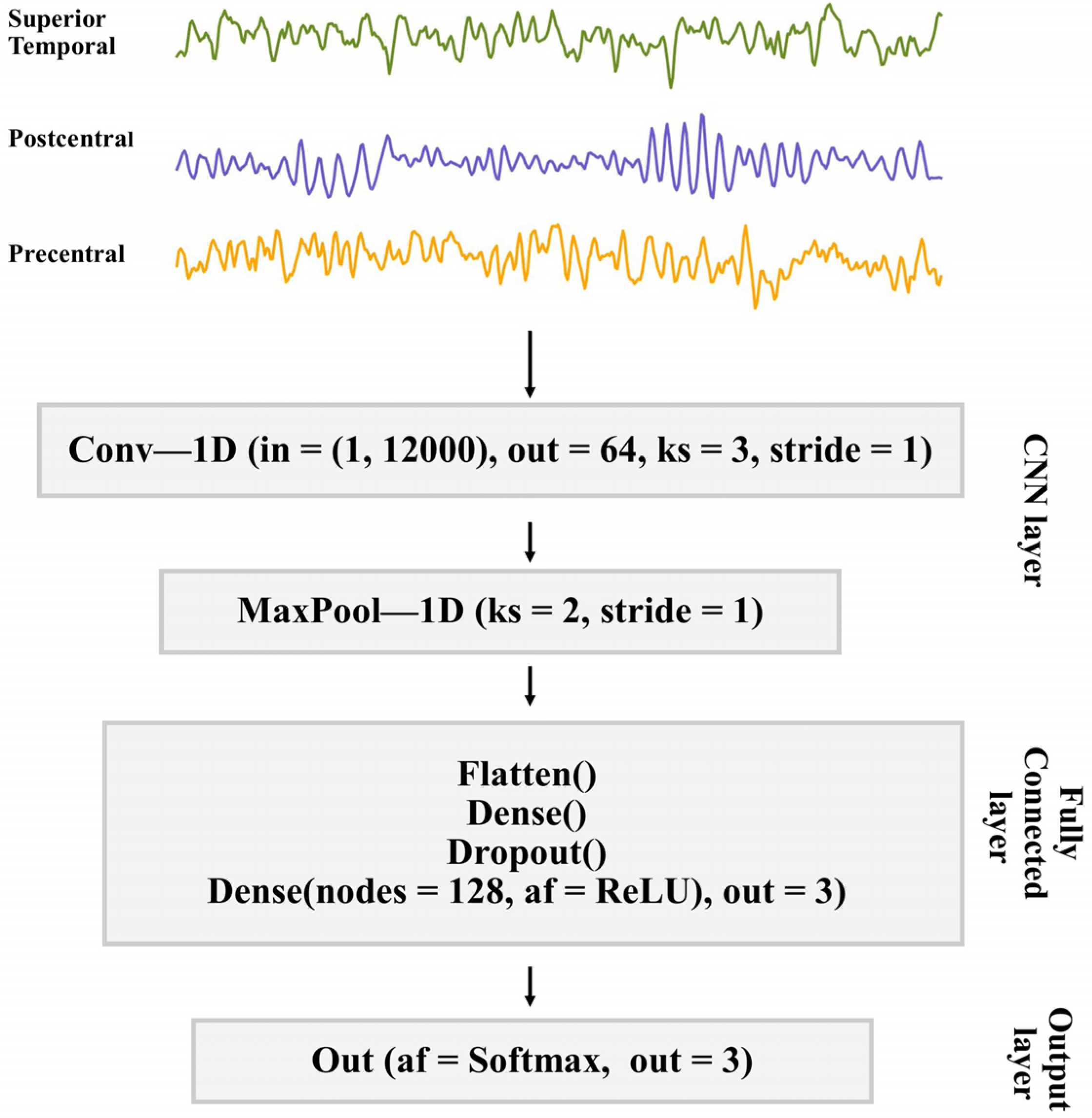
Having analysed that the differences between the sEEG signals from the three gyri can be detected with well-defined spectral and fractal deterministic methods, we investigated the ability to reveal the cortical parcel features, and to perform an automatic classification with machine learning techniques in the time domain. For this analysis, we deployed two models. Initially, we used the one-dimensional convolutional neural network (1D-CNN), which bases the prediction of the groups on the features extracted from the signals. And we also deploy a one-shot learning model, which learns the features of the signal from one or a few examples from a group, by calculating the distance between pairs of samples from different groups.

2.4. 1D-CNN Model

Many authors report that 1D-CNNs outperform the state-of-the-art machine learning models and achieve high accuracy in classifying time series, even though they express chaotic behaviour, which would demonstrate the effectiveness of CNNs in capturing complex patterns and generalising to different types of time series data [30,31,32,33]. To find out if it will be effective for classifying sEEG signals from different cortical sources, we implemented a 1D-CNN connected with a max-pooling layer. We added one layer that is fully connected with a rectified linear unit (ReLU) activation function, and an output layer that is activated with a Softmax function, where the output layer provides the probability of the three classes needed for recognizing the sources we are investigating. For the assessment of the loss, we used the categorical cross-entropy function. The network was trained on 60 s long temporal sEEG time series from three groups, where one example of data was one sEEG channel from a specific gyrus. The training set included 70% of the data. The training was performed for 50 epochs. The 1D-CNN model was built with the parameters depicted in Figure 2.

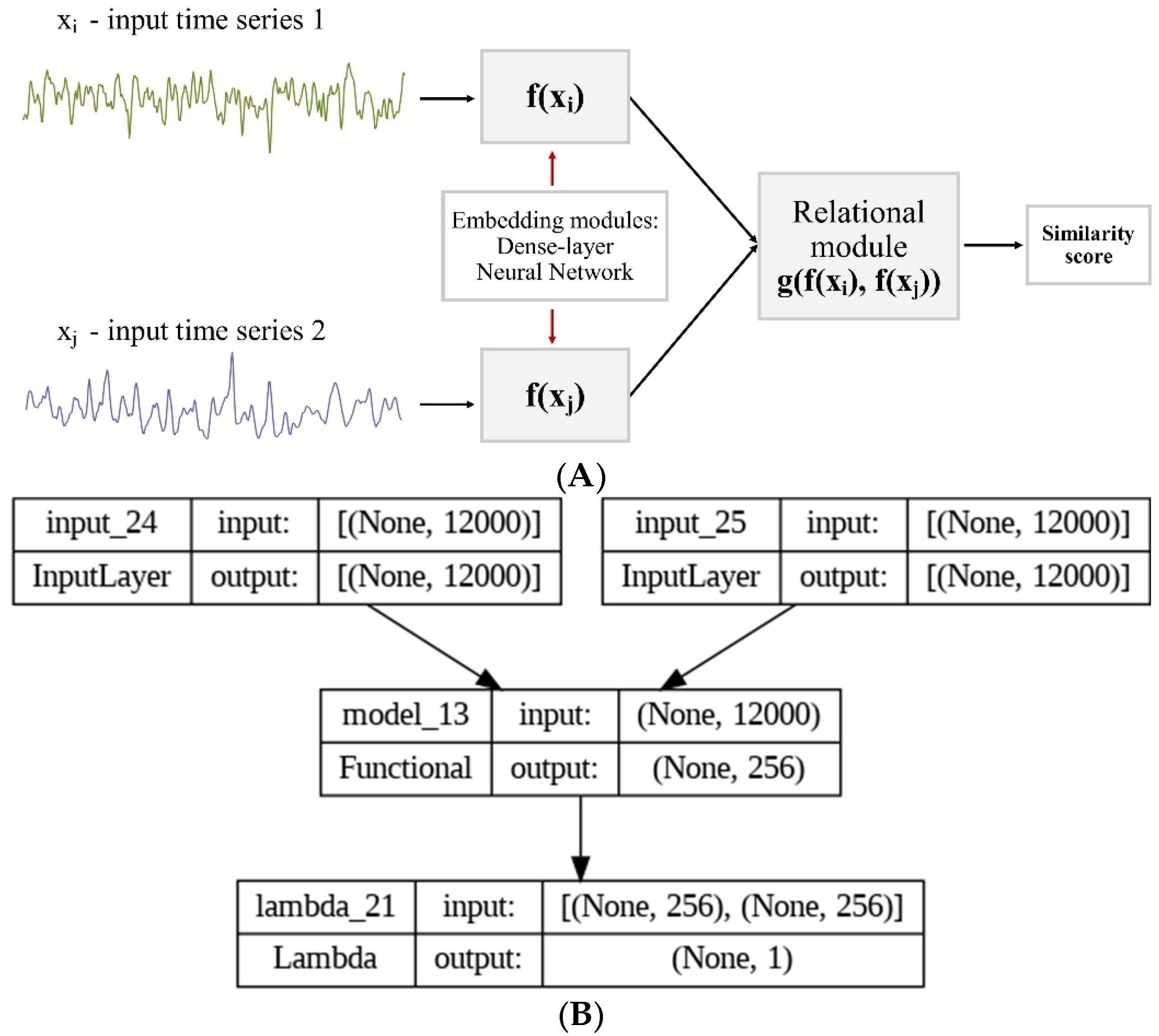
2.5. One-Shot Learning Model

Even though the 1D-CNN is a plausible method in classification tasks of temporal series, we encountered several problems by applying it for classifying the signals of the investigated cortical areas. In fact, the number of sEEG recordings is limited with respect to the necessary number to train the network, and the number of available channels is not homogenous in the three areas, which can introduce bias into the training. To solve these issues, we deployed a one-shot learning model, which learns to compare by measuring the similarity between pairs of inputs and should be immune to the non-homogeneity of the number of samples between classes. The neural network architecture that we deployed is called “Siamese”, and it comes from the idea that the network consists of two identical subnetworks that share weights and parameters [34]. These subnetworks process two input examples and extract feature vectors, named embeddings. The embeddings are then compared using a distance metric to determine the similarity between the inputs [35]. By training the network on pairs of examples, each belonging to two different classes, the network learns to discriminate between different classes based on their similarity. This allows the network to generalize to new examples by making predictions based on a single example [35]. In Figure 3A, we provide a schematic representation of the one-shot learning neural network architecture; in Figure 3B, the parameters used are presented. The module that extracts the embeddings from the time series is the dense layer of the neural network, while the embeddings are submitted to the relational module, which calculates the distance metric between them. For our architecture, we selected the cosine distance:

$$\mathrm{S}\mathrm{i}\mathrm{m}\mathrm{i}\mathrm{l}\mathrm{a}\mathrm{r}\mathrm{i}\mathrm{t}\mathrm{y} \mathrm{s}\mathrm{c}\mathrm{o}\mathrm{r}\mathrm{e}=\cos \left(\phi \right)={\displaystyle \frac{A·B}{‖A‖‖B‖}}$$

where A and B are the embeddings or feature vectors of the two compared signals, and ‖A‖ and ‖B‖ represent their Euclidean (L2) norms.

2.6. Statistical Analysis

In the comparison of the mean band PSD and Higuchi fractal dimension of the cortical areas, in order to verify the significance of the differences pointed out between the groups, we deployed an independent Kruskal–Wallis-test, hereafter H_test, that does not assume the normal distribution of the data. For simplicity, when both comparisons were significant, we reported the less significant one. Statistical significance was set to p ≤ 0.05. For the machine learning classification, we provide the metrics such as training and testing accuracy, precision, recall, and f1 score.

3. Results

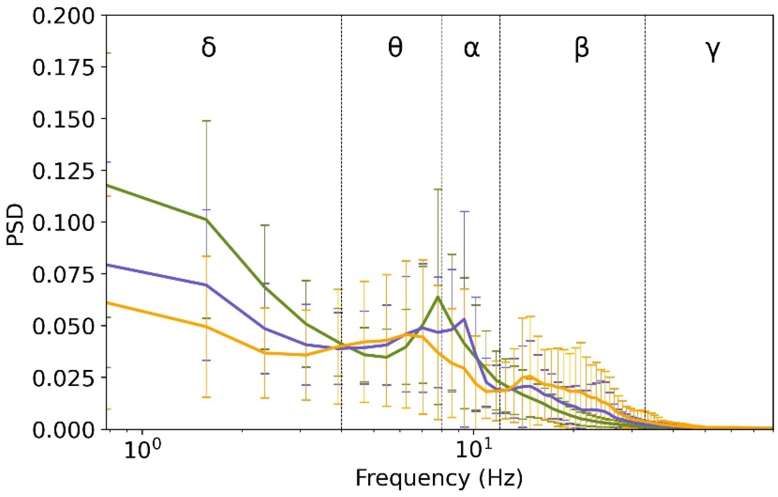
3.1. Spectral Features in the Three Cortical Parcels

In agreement with previous studies [4,24,36], we find that different cortical parcels express their own characteristic and distinctive oscillatory activity (Figure 4). In particular, we pointed out that, in the delta frequency band, the PSD in superior temporal gyrus is higher than in the other two gyri (p < 0.01). We also observe that the precentral gyrus has a higher PSD than the other two gyri, both in the beta frequency band (p < 0.01) and in the gamma band (p ≤ 0.07). Then, we observe that in the alpha frequency band, the postcentral gyrus PSD is higher only than the precentral gyrus (H_test = 22.84, p = 1.76 × 10⁻⁶). We did not find any differences between the three gyri in the theta frequency band (p > 0.07). In Figure 5, we provide a visualisation of the differences of the mean band PSD between the three cortical areas by plotting the spatial distribution of the band PSD in each channel, averaging the PSD in a given frequency band, from δ (top panel) to γ (bottom panel).

3.2. Higuchi Fractal Dimension in the Three Cortical Parcels

A fractality measure that we deployed for researching the differences between the cortical parcels is the HFD. We found significant differences: the HFD of the neurodynamics is higher in the precentral gyrus than that in the postcentral gyrus (H_test = 12.62, p = 3.82 × 10⁻⁴) and the HFD in postcentral gyrus is higher than that in the superior temporal gyrus (H_test = 20.05, p = 7.54 × 10⁻⁶). Differences can be inspected in Figure 6. Significantly, this result could suggest that (i) the HFD measure is effective in catching the existence of complexity features in the three cortical areas; (ii) it allows us to statistically distinguish the parcels between them.

3.3. The Classification of the Three Cortical Parcels with 1D-CNN Model

As a first step, to evaluate the performance of a state-of-the-art neural network in automatically classifying signals from three different cortical areas, we implemented a 1D-CNN. The results summarized in

Table 1. Metrics by classes of the 1D-CNN in the training and test sets.

	Class	Precision (%)	Recall (%)	F1 Score (%)
Train	PreCG	89	100	94
	PostCG	69	93	80
	STG	100	51	67
Test	PreG	50	72	57
	PostG	30	30	30
	STG	100	0	0

suggest that the neural network is capable of identifying distinct patterns across the three groups and correctly labelling them within the training set. However, the model demonstrates a limited generalization ability when applied to unseen data. Moreover, the test set results reveal a pronounced bias toward the group with a lower number of examples, specifically, the postcentral gyrus with only 64 channels. As a result, this group shows the lowest performance metrics. Overall, the evaluation of the 1D-CNN performance on both the training and test sets (

Table 2. Overall metrics of the 1D-CNN for the training and test sets.

	Method	Precision (%)	Recall (%)	F1 Score (%)	Accuracy (%)
Train	Macro avg	86	81	80	85
	Weighted avg	88	85	83
Test	Macro avg	58	34	29	50
	Weighted avg	57	43	35

) is promising, given the difficulty of the task for such a simple neural network. The model achieved an accuracy of 85% on the training set and 50% on the test set.

3.4. Classification of the Three Cortical Parcels with One-Shot Learning Model

The 1D-CNN architecture requires a large amount of data and homogenous distribution between classes; due to these limitations, we implemented an alternative one-shot learning architecture. This model may offer advantages over traditional deep learning approaches, as it is designed to learn from few samples within each class. The one-shot learning architecture captures the within-group and between-group differences. The results, summarized in

Table 3. The overall metric of the one-shot learning architecture for training and test sets.

	Method	Precision (%)	Recall (%)	F1 Score (%)	Accuracy
Train	Macro avg	63	56	55	58
	Weighted avg	63	56	55
Test	Macro avg	58	56	54	56
	Weighted avg	58	56	54

, indicate that the one-shot learning architecture has potential for generalizing the features of the signal. The overall accuracy for the training and test sets are 58% and 56%, respectively.

4. Discussion

In this analysis, we studied several statistical and machine learning methods to classify the neurodynamics of distinct cerebral cortex parcels during the resting state in wakefulness, using intracranial stereo-electroencephalographic recordings. Our spectral analysis has shown that the cortical areas exhibit particular oscillatory activity that allows for distinguishing between the precentral, postcentral, and superior temporal gyri, supporting results from previous studies [4,36]. In these studies, authors demonstrated that the neurodynamics of different cortical areas in resting wakefulness exhibit characteristic behaviours that can be considered as fingerprints of those areas by analysing MEG [36] and sEEG recordings [4] in various brain regions. In both studies [4,36], to characterize the features of ongoing brain electrical activity, the authors examined the Power Spectral Density (PSD) function. They reported that alpha rhythms (8–12 Hz) are predominantly found in the occipital lobe, parietal lobe, and temporal lobes, while beta rhythms (12–33 Hz) are frequently found in the anterior head regions. Well-sustained beta frequencies prevail in the precentral and postcentral gyri, with peaks at lower frequencies in the postcentral region, while the precentral gyrus also expresses gamma (33–100 Hz) activity. Our results in PSD align with those from the aforementioned studies.

Traditional linear analysis methods provide significant insights into harmonic brain activity, but they may not fully capture the inherently non-linear spectrum of brain dynamics. Studies suggest that during wakefulness and in the resting state, neurodynamics are highly structured [37] and behave in a correlated manner, forming a rich temporal dynamical pattern [17,38,39]. This dynamic pattern is present regardless of the monitoring method, whether measuring electrical activity on the scalp (EEG), intracranial stereotactic electroencephalography (sEEG), or using techniques such as functional magnetic resonance imaging (fMRI) [28,37]. This structured pattern exhibits a fractal [40] and scale-free [41] behaviour. Therefore, to detect the differences between the cortical parcels, we also deployed fractality measures, such as the Higuchi fractal dimension. It has shown to be sensitive to the features of complexity of the signals that allow for distinguishing cortical parcels between them, with a higher complexity expressed in the precentral gyrus, a lower complexity in the postcentral gyrus, and an even lower complexity than the latter in the superior temporal gyrus. This finding is in line with the analyses conducted in previous similar studies to compare the complexity of different brain regions [7,10,24,28,42]. Such results imply that fractal dimension measures could be a marker to identify a cortical parcel from its ongoing electrical activity in a resting state. Such fractality can be revealed from both the scalp electroencephalography [28] and intracranial recordings [4], but the latter provides more precise signals directly from the location, avoiding the signal filtering with extracortical tissues and the skull.

Furthermore, we tested how some machine learning methods, which intrinsically could be less deterministic, would achieve similar results in classifying the investigated areas. In fact, deploying two deep learning architectures, a 1D-CNN and a one-shot learning model, we achieved results that might appear less significant than the deterministic methods, but are still promising. The 1D-CNN showed a plausible performance on the training set, with an 85% accuracy, but failed to generalize on the test set. This performance might have occurred due to at least a couple of reasons: (i) too low number of samples for training the network; (ii) a possible bias due to the non-equal number of samples in the classes. Because of these issues of the 1D-CNN, we proceeded with another architecture, which should have solved the problem of the scarcity of data. The one-shot learning architecture has been shown to perform well in signature recognition [43], material classification [44], or even epileptic seizure detection [45], even with a limited number of samples. Also, in our case, the one-shot learning architecture has shown advantages over the 1D-CNN architecture in the generalization of the learned features on the test set, by achieving a nearly 60% accuracy. The difficulty of such classifications in the time series, directly in the time domain, lies in the huge variability of the electrode location within each cortical parcel, the variability between the subjects, and the closeness of some contacts to the boundary between two areas. While there are studies that have classified the EEG resting state recordings in order to distinguish Alzheimer’s disease and frontotemporal lobe dementia patients [46] or Parkinson’s disease and Schizophrenia patients [47], the attempts to classify brain parcels with neural networks seem to be scarce [36].

Limitations of This Study and Future Developments

Despite the insights into a possible characteristic signature of the neurodynamics of the cortical parcels, this study has limitations. One of the limits is in the fractality measurement methods. The numerical estimation of the HFD measure depends on tuneable parameters, which could impact the final value of the measure. However, we did not aim to investigate the absolute value of the fractal dimension of the signals, but we adopted a more conservative and pragmatic approach by considering the HFD as an index able to classify the temporal series. For this reason, we followed the literature and implemented the calculation accordingly, by selecting a k_max value equal to 35 for the HFD, as described in [24].

Another limit, mainly for machine learning classification, is the sparse number of the channels from the three cortical parcels investigated. In particular, we possessed only 64 channels from the postcentral gyrus, which is a rather low number for the traditional neural network. This could have been the reason why the 1D-CNN encountered a low achievement in the classification of the test set.

Furthermore, despite the potentiality of the application of the one-shot learning model in various fields for classification tasks, it may struggle with datasets where the intra-class variations are high. In this particular case, the intra-class variability is occurring due to the wide distribution of the channels in one parcel that come from different subjects. In this way, we introduce not only intra-subject variability but also a inter-subject variability [48]. Also, the one-shot learning network can be computationally expensive to train.

Having observed that spectral and fractal measures can be capable of detecting the differences between the neurodynamics of cortical areas, we aim at developing an automatic machine learning tool that could be able to achieve a higher accuracy classification of the signals from different cortical areas. The integration of the fractal measure and one-shot learning could help to achieve higher performance in signal classification.

5. Conclusions

In this study, we explored the potential of deep learning models to classify cortical regions based on neurodynamic features rather than traditional cytoarchitectonic distinctions. Our results indicate that while one-shot learning networks offer certain advantages, they struggle to distinguish cortical parcels effectively, as evidenced by their inability to recognize time series patterns, even during training. Conversely, convolutional neural networks (CNNs) demonstrate more adequacy, achieving over an 85% accuracy in the training set. However, despite this improvement, our findings suggest that current network architectures still lack the necessary integration of structural and process-based measures required for precise classification.

The implications of this research extend to the possibility of classifying cortical regions through their neurodynamic behaviour, paving the way for novel neuromodulation approaches that could interact with brain activity in unprecedented ways. While our current models do not yet achieve this level of classification, our findings highlight that deep learning approaches can be a promising pathway for achieving this aim. Further advancements in model design and the incorporation of more refined neurodynamic features will be crucial in progressing toward this goal. In the direction of feature selection, we confirm the relevance of using the whole time behaviour of the neuronal electrical activity, with the Higuchi fractal dimension being much more promising than linear measures like PSD.

References

1. Tecchio, F.; Bertoli, M.; Gianni, E.; L’Abbate, T.; Paulon, L.; Zappasodi, F. To Be Is To Become. Fractal Neurodynamics of the Body-Brain Control System. Front. Physiol. 2020, 11, 609768. [Google Scholar] [CrossRef]
2. Li, J. Thoughts on neurophysiological signal analysis and classification. Brain Sci. Adv. 2020, 6, 210–223. [Google Scholar] [CrossRef]
3. Moaveninejad, S.; D’Onofrio, V.; Tecchio, F.; Ferracuti, F.; Iarlori, S.; Monteriù, A.; Porcaro, C. Fractal Dimension as a discriminative feature for high accuracy classification in motor imagery EEG-based brain-computer interface. Comput. Methods Programs Biomed. 2024, 244, 107944. [Google Scholar] [CrossRef] [PubMed]
4. Frauscher, B.; Von Ellenrieder, N.; Zelmann, R.; Doležalová, I.; Minotti, L.; Olivier, A.; Hall, J.; Hoffmann, D.; Nguyen, D.K.; Kahane, P.; et al. Atlas of the normal intracranial electroencephalogram: Neurophysiological awake activity in different cortical areas. Brain 2018, 141, 1130–1144. [Google Scholar] [CrossRef] [PubMed]
5. Ruiz de Miras, J.; Soler, F.; Iglesias-Parro, S.; Ibáñez-Molina, A.J.; Casali, A.G.; Laureys, S.; Massimini, M.; Esteban, F.J.; Navas, J.; Langa, J.A. Fractal dimension analysis of states of consciousness and unconsciousness using transcranial magnetic stimulation. Comput. Methods Programs Biomed. 2019, 175, 129–137. [Google Scholar] [CrossRef]
6. Yoder, K.J.; Brookshire, G.; Glatt, R.M.; Merrill, D.A.; Gerrol, S.; Quirk, C.; Lucero, C. Fractal Dimension Distributions of Resting-State Electroencephalography (EEG) Improve Detection of Dementia and Alzheimer’s Disease Compared to Traditional Fractal Analysis. Clin. Transl. Neurosci. 2024, 8, 27. [Google Scholar] [CrossRef]
7. Armonaite, K.; Conti, L.; Olejarczyk, E.; Tecchio, F.; Roma, S.; Vergata, T. Insights on neural signal analysis with Higuchi fractal dimension. Commun. Appl. Ind. Math. 2024, 15, 17–27. [Google Scholar] [CrossRef]
8. Kesić, S.; Spasić, S.Z. Application of Higuchi’s fractal dimension from basic to clinical neurophysiology: A review. Comput. Methods Programs Biomed. 2016, 133, 55–70. [Google Scholar] [CrossRef]
9. Higuchi, T. Approach to an irregular time series on the basis of the fractal theory. Phys. D Nonlinear Phenom. 1988, 31, 277–283. [Google Scholar] [CrossRef]
10. Olejarczyk, E.; Gotman, J.; Frauscher, B. Region-specific complexity of the intracranial EEG in the sleeping human brain. Sci. Rep. 2022, 12, 451. [Google Scholar] [CrossRef]
11. Salimi, M.; Tabasi, F.; Abdolsamadi, M.; Dehghan, S.; Dehdar, K.; Nazari, M.; Javan, M.; Mirnajafi-Zadeh, J.; Raoufy, M.R. Disrupted connectivity in the olfactory bulb-entorhinal cortex-dorsal hippocampus circuit is associated with recognition memory deficit in Alzheimer’s disease model. Sci. Rep. 2022, 12, 4394. [Google Scholar] [CrossRef] [PubMed]
12. Chen, X.Y.; Liu, C.; Xue, Y.; Chen, L. Changed firing activity of nigra dopaminergic neurons in Parkinson’s disease. Neurochem. Int. 2023, 162, 105465. [Google Scholar] [CrossRef]
13. Nasca, C.; Barnhill, O.; DeAngelis, P.; Watson, K.; Lin, J.; Beasley, J.; Young, S.P.; Myoraku, A.; Dobbin, J.; Bigio, B.; et al. Multidimensional predictors of antidepressant responses: Integrating mitochondrial, genetic, metabolic and environmental factors with clinical outcomes. Neurobiol. Stress 2021, 15, 100407. [Google Scholar] [CrossRef] [PubMed]
14. Wang, Z.; Chen, L.M.; Négyessy, L.; Friedman, R.M.; Mishra, A.; Gore, J.C.; Roe, A.W. The Relationship of Anatomical and Functional Connectivity to Resting-State Connectivity in Primate Somatosensory Cortex. Neuron 2013, 78, 1116–1126. [Google Scholar] [CrossRef]
15. Economo, M.N.; Viswanathan, S.; Tasic, B.; Bas, E.; Winnubst, J.; Menon, V.; Graybuck, L.T.; Nguyen, T.N.; Smith, K.A.; Yao, Z.; et al. Distinct descending motor cortex pathways and their roles in movement. Nature 2018, 563, 79–84. [Google Scholar] [CrossRef]
16. Greicius, M.D.; Krasnow, B.; Reiss, A.L.; Menon, V. Functional connectivity in the resting brain: A network analysis of the default mode hypothesis. Proc. Natl. Acad. Sci. USA 2003, 100, 253–258. [Google Scholar] [CrossRef]
17. Raichle, M.E.; Macleod, A.M.; Snyder, A.Z.; Powers, W.J.; Gusnard, D.A.; Shulman, G.L. A default mode of brain function. Proc. Natl. Acad. Sci. USA 2001, 98, 676–682. [Google Scholar] [CrossRef]
18. von Ellenrieder, N.; Gotman, J.; Zelmann, R.; Rogers, C.; Nguyen, D.K.; Kahane, P.; Dubeau, F.; Frauscher, B. How the Human Brain Sleeps: Direct Cortical Recordings of Normal Brain Activity. Ann. Neurol. 2020, 87, 289–301. [Google Scholar] [CrossRef]
19. Solomon, M.O. PSD Computations Using Welch’s Method. Sandia Natl. Lab. 1991, 64, 23584. [Google Scholar]
20. Spasić, S.; Kalauzi, A.; Ćulić, M.; Grbić, G.; Martać, L. Estimation of parameter kmax in fractal analysis of rat brain activity. Ann. N. Y. Acad. Sci. 2005, 1048, 427–429. [Google Scholar] [CrossRef]
21. Paramanathan, P.; Uthayakumar, R. Application of fractal theory in analysis of human electroencephalographic signals. Comput. Biol. Med. 2008, 38, 372–378. [Google Scholar] [CrossRef]
22. Smits, F.M.; Porcaro, C.; Cottone, C.; Cancelli, A.; Rossini, P.M.; Tecchio, F. Electroencephalographic Fractal Dimension in Healthy Ageing and Alzheimer’s Disease. PLoS ONE 2016, 11, e0149587. [Google Scholar] [CrossRef]
23. Armonaite, K.; Nobili, L.; Paulon, L.; Balsi, M.; Conti, L.; Tecchio, F. Local neurodynamics as a signature of cortical areas: New insights from sleep. Cereb. Cortex 2022, 33, 3284–3292. [Google Scholar] [CrossRef] [PubMed]
24. Armonaite, K.; Bertoli, M.; Paulon, L.; Gianni, E.; Balsi, M.; Conti, L.; Tecchio, F. Neuronal Electrical Ongoing Activity as Cortical Areas Signature: An Insight from MNI Intracerebral Recording Atlas. Cereb. Cortex 2021, 32, 2895–2906. [Google Scholar] [CrossRef]
25. Liehr, L.; Massopust, P. On the mathematical validity of the Higuchi method. Phys. D Nonlinear Phenom. 2020, 402, 132265. [Google Scholar] [CrossRef]
26. Ahmadlou, M.; Adeli, H.; Adeli, A. Fractality analysis of frontal brain in major depressive disorder. Int. J. Psychophysiol. 2012, 85, 206–211. [Google Scholar] [CrossRef]
27. Phinyomark, A.; Larracy, R.; Scheme, E. Fractal Analysis of Human Gait Variability via Stride Interval Time Series. Front. Physiol. 2020, 11, 333. [Google Scholar] [CrossRef] [PubMed]
28. Cottone, C.; Porcaro, C.; Cancelli, A.; Olejarczyk, E.; Salustri, C.; Tecchio, F. Neuronal electrical ongoing activity as a signature of cortical areas. Brain Struct. Funct. 2017, 222, 2115–2126. [Google Scholar] [CrossRef]
29. Olejarczyk, E.; Zappasodi, F.; Ricci, L.; Pascarella, A.; Pellegrino, G.; Paulon, L.; Assenza, G.; Tecchio, F. Functional Source Separation-Identified Epileptic Network: Analysis Pipeline. Brain Sci. 2022, 12, 1179. [Google Scholar] [CrossRef]
30. Yang, B.; Zhu, X.; Liu, Y.; Liu, H. A single-channel EEG based automatic sleep stage classification method leveraging deep one-dimensional convolutional neural network and hidden Markov model. Biomed. Signal Process. Control 2021, 68, 102581. [Google Scholar] [CrossRef]
31. Cisotto, G.; Zanga, A.; Chlebus, J.; Zoppis, I.; Manzoni, S.; Markowska-Kaczmar, U. Comparison of Attention-based Deep Learning Models for EEG Classification. arXiv 2020, arXiv:2012.01074. [Google Scholar]
32. Ullah, I.; Hussain, M.; Qazi, E.-U.-H.; Aboalsamh, H. An automated system for epilepsy detection using EEG brain signals based on deep learning approach. Expert Syst. Appl. 2018, 107, 61–71. [Google Scholar] [CrossRef]
33. Truong, N.D.; Nguyen, A.D.; Kuhlmann, L.; Bonyadi, M.R.; Yang, J.; Ippolito, S.; Kavehei, O. Convolutional neural networks for seizure prediction using intracranial and scalp electroencephalogram. Neural Netw. 2018, 105, 104–111. [Google Scholar] [CrossRef]
34. Wu, X.; Kimura, A.; Iwana, B.K.; Uchida, S.; Kashino, K. Deep dynamic time warping: End-to-end local representation learning for online signature verification. In Proceedings of the 2019 International Conference on Document Analysis and Recognition (ICDAR), Sydney, Australia, 20–25 September 2019; pp. 1103–1110. [Google Scholar]
35. Wang, X.; Sun, K.; Zhao, T.; Wang, W.; Gu, Q. Dynamic Speed Warping: Similarity-Based One-shot Learning for Device-free Gesture Signals. In Proceedings of the IEEE INFOCOM 2020-IEEE Conference on Computer Communications, Toronto, ON, Canada, 6–9 July 2020; pp. 556–565. [Google Scholar]
36. Keitel, A.; Gross, J. Individual Human Brain Areas Can Be Identified from Their Characteristic Spectral Activation Fingerprints. PLoS Biol. 2016, 14, e1002498. [Google Scholar] [CrossRef] [PubMed]
37. Barttfeld, P.; Uhrig, L.; Sitt, J.D.; Sigman, M.; Jarraya, B. Signature of consciousness in the dynamics of resting-state brain activity. Proc. Natl. Acad. Sci. USA 2015, 112, 887–892. [Google Scholar] [CrossRef]
38. Fox, M.D.; Raichle, M.E. Spontaneous fluctuations in brain activity observed with functional magnetic resonance imaging. Nat. Rev. Neurosci. 2007, 8, 700–711. [Google Scholar] [CrossRef]
39. He, B.J.; Zempel, J.M.; Snyder, A.Z.; Raichle, M.E. The temporal structures and functional significance of scale-free brain activity. Neuron 2010, 66, 353–369. [Google Scholar] [CrossRef] [PubMed]
40. Di Ieva, A.; Grizzi, F.; Jelinek, H.; Pellionisz, A.J.; Losa, G.A. Fractals in the neurosciences, part I: General principles and basic neurosciences. Neuroscientist 2014, 20, 403–417. [Google Scholar] [CrossRef]
41. Muthukumaraswamy, S.D.; Liley, D.T. 1/F Electrophysiological Spectra in Resting and Drug-Induced States Can Be Explained By the Dynamics of Multiple Oscillatory Relaxation Processes. Neuroimage 2018, 179, 582–595. [Google Scholar] [CrossRef]
42. Armonaite, K.; Conti, L.; Tecchio, F. Fractal Neurodynamics; Springer: Berlin/Heidelberg, Germany, 2024; Volume 36. [Google Scholar]
43. VAROL ARISOY, M. Signature Verification Using Siamese Neural Network One-Shot Learning. Int. J. Eng. Innov. Res. 2021, 3, 248–260. [Google Scholar] [CrossRef]
44. Weis, J.; Santra, A. One-shot learning for robust material classification using millimeter-wave radar system. IEEE Sensors Lett. 2018, 2, 2–5. [Google Scholar] [CrossRef]
45. Burrello, A.; Schindler, K.; Benini, L.; Rahimi, A. One-shot Learning for iEEG Seizure Detection Using End-to-end Binary Operations: Local Binary Patterns with Hyperdimensional Computing. In Proceedings of the 2018 IEEE Biomedical Circuits and Systems Conference (BioCAS), Cleveland, OH, USA, 17–19 October 2018; pp. 1–4. [Google Scholar]
46. Jiang, R.; Zheng, X.; Sun, J.; Chen, L.; Xu, G.; Zhang, R. Classification for Alzheimer’s disease and frontotemporal dementia via resting-state electroencephalography-based coherence and convolutional neural network. Cogn. Neurodyn. 2025, 19, 46. [Google Scholar] [CrossRef] [PubMed]
47. Xiong, W.; Ma, L.; Li, H. Efficient Neural Network Classification of Parkinson’s Disease and Schizophrenia Using Resting-State EEG Data. Brain Topogr. 2025, 38, 32. [Google Scholar] [CrossRef]
48. Saha, S.; Baumert, M. Intra- and Inter-subject Variability in EEG-Based Sensorimotor Brain Computer Interface: A Review. Front. Comput. Neurosci. 2020, 13, 87. [Google Scholar] [CrossRef] [PubMed]
Figure 1. Spatial distribution of the position of the sEEG electrodes. Recordings collected from precentral gyrus (orange, central-anterior part of the brain), postcentral gyrus (purple, central-posterior part of the brain), superior temporal gyrus (green, lateral-inferior part of the brain) are presented in four brain projections. L and R letters stands for left and right hemispheres, respectively, from total 55 subjects.
Fractalfract 09 00278 g001
Figure 2. Schematic representation of the 1D-CNN implemented architecture. From top to bottom: example of temporal series from STG (green), postCG (purple), and preCG (orange) given to the network as input. Grey rectangles represent the network layers: 1-dimensional convolutional layer (Conv-1D), with the specified hyperparameters in—the size of a single time series, out—number of the feature maps resulting from the convolution operation with the kernel/filter, which size is ks, and stride—size of the convolution step. One-dimensional max-pooling layer (MaxPool-1D). Fully connected layer (FC). The size of the Flatten() is determined by the size MaxPool1D output. Dense() and Dropout() are hidden layers, with af—activation function, which in our case is a rectified linear unit (ReLU) for hidden dense layers, and Softmax for output layer.
Fractalfract 09 00278 g002
Figure 3. Schematic representation of the one-shot learning neural network architecture. (A). The symbols xi and xj are the compared input time series from two different gyri. The embedding module is the dense-layer neural network for feature detection (see architecture in Figure 2). The symbols f(xi) and f(xj) indicate the feature vector learned from the embedded neural network. The relational module is represented by the function g(f(xi), f(xj)), which calculates the cosine distances between the two features vectors. The output module provides the similarity score. (B). The same one-shot learning architecture is presented with input shapes in the network. To train the Siamese network, pairs of inputs along with their tagging labels (the cortical areas) are required. The model receives two input vectors, each with a length of 12,000, representing two distinct examples. Both inputs are processed through a shared subnetwork, which maps each input to a 256-dimensional feature vector. This shared feature extractor ensures that the same weights are applied to both inputs. The 256-dimensional embeddings are then compared in the Lambda layer, which computes a similarity score by evaluating the distance or difference between the two vectors. The final output is a single scalar value representing the degree of similarity between the two inputs, with values indicating how closely related they are.
Fractalfract 09 00278 g003
Figure 4. The mean PSD for the three gyri. Mean and standard deviation of PSD averaged across all channels separately for the three cortical parcels are given. Green line stands for superior temporal gyrus, purple line for postcentral gyrus, and orange one for precentral gyrus. This shows that the three regions of investigation express characteristic oscillatory activity in a certain band. STG in δ band, PostCG in α band, and PreCG β, γ bands.
Fractalfract 09 00278 g004
Figure 5. PSD distribution across the three gyri. Graphic representation in the three coronal, sagittal, and axial projections of the PSD values of the channel in the five frequency bands from δ (top) to γ (bottom). Each point represents a recording channel, and the colour indicates the band PSD value according to the reproduced scale (appropriate values for each band). It can be noted that the PSD is more intense in the δ band in the STG, in β in the postCG, and in γ in the preCG.
Fractalfract 09 00278 g005
Figure 6. Spatial map and distribution of HFD for the three cortical parcels. (Left) The HFD value of each sEEG channel mapped on the brain contour, in the three spatial projections, located according to the coordinates of the channel. Higher HFD values are seen in the precentral gyrus. (Right) The boxplots of the HFD for the three cortical parcels showing the mean and the standard deviation for STG (superior temporal gyrus), PostCG (postcentral gyrus), and PreCG (precentral gyrus). The small triangular shapes represent the HFD for each channel shifted horizontally for increased readability.
Fractalfract 09 00278 g006