Abstract
This work presents and compares different methodologies for the joint optimisation of the fractional derivative order and the parameters of the right-hand-side neural network in Neural Fractional Differential Equation models. The proposed strategies aim to tackle the training difficulties typically encountered when learning the fractional order together with the network weights. One approach is based on regulating the gradient magnitude of the loss function with respect to , encouraging more stable and effective updates. Another strategy introduces an online pre-training scheme, where the network parameters are initially optimised over progressively longer time intervals, while is updated more conservatively using the full time trajectory. The study focuses only on a foundational setting with one-dimensional problems, and numerical experiments demonstrate that the proposed techniques improve both training stability and accuracy. Nonetheless, the issue of non-uniqueness in the optimal derivative order remains, particularly in less well-posed scenarios, suggesting the need for further research in data-driven modelling of fractional-order systems.
1. Introduction
Neural Fractional Differential Equations (Neural FDEs) form a class of neural architectures aimed at approximating solutions for time-dependent data , where each represents data collected at time , typically from experiments or simulations over a time interval [1,2]. Neural FDEs have attracted attention and are currently an emerging architecture in the literature, with extensions to Graph Neural Networks [3], variable-order operators [4], integrating physical knowledge [5], and more efficient adjoint algorithms to accelerate training [6]. While Neural FDEs can also be applied to model problems beyond time-series data, such applications are beyond the scope of this work [7].
These models incorporate a fractional derivative of Caputo type (the Caputo derivative definition is used due to its popularity in real-world formulations as it uses integer-order initial conditions) [8,9] (or any other fractional derivative [10,11,12,13,14,15,16]), denoted , into a neural network-driven dynamical system:
where is a neural network with parameters , and is the order of the fractional derivative. The Caputo fractional derivative for a scalar function with is defined as follows:
with representing the Gamma function .
A remarkable feature of this framework is the flexibility to learn not only the network parameters but also the fractional order . When , the formulation recovers the well-known Neural ODEs [17].
In the approach proposed in [2], the fractional order is parametrised by a dedicated neural network, denoted by , with trainable parameters . This formulation is especially advantageous when dealing with systems where the fractional order of differentiation is a function of time, accommodating non-stationary dynamics. It is worth noting that, when is constant, it can be treated as a single trainable parameter of the model, rather than being represented by a neural network, as is done in this work. Thus, learning involves jointly optimising and (or ) by minimising the difference between the predicted trajectory (obtained from the numerical solution of (1)) and the true data ; that is:
where is the norm.
Here, denotes an appropriate numerical solver for the Fractional Differential Equation (FDE) (1) (see [2] for more details), and the loss function is defined as the Mean Squared Error (MSE) between the model prediction and the observed data.
Although the study in [2] reports that the fractional order can be inferred from data for various datasets, the estimated values often differ significantly from the true (ground-truth) values, and different initialisations of lead to different optimal values.
Building upon this, the work in [18] further investigated numerically the dependency between and , showing that the neural network in the right-hand side of the Neural FDE struggles to consistently adjust its parameters to accurately represent the system’s dynamics for arbitrary values of . As a result, Neural FDEs do not necessarily converge to a unique optimal fractional order; instead, they may rely on a wide range of values to achieve a reasonable fit to the data. This flexibility, however, comes at a cost. Every time the value of is modified during training, the underlying function must be re-learnt, as the optimal parameter set for one fractional order might differ substantially from that of another. This results in an inefficient and potentially unstable optimisation process, since the function learnt by the network may change substantially with small variations in .
To better understand the complex dependence of the neural network on the order of the derivative, it is helpful to first examine an analytical problem (specifically, a fractional initial value problem) for which there are known results concerning the continuity of the solution with respect to the problem data [9,19]:
Theorem 1.
Let , , and . Consider the Caputo fractional initial-value problem
and two perturbed problems on the same interval :
where satisfies the same Lipschitz (with respect to the second variable) and continuity hypotheses as f, and ε is a small scalar perturbation of the derivative order.
Define
with D a suitable domain where the solution exists and is unique. Then, there exists and a constant such that the unique solutions , and exist on and satisfy
or,
This means that small perturbations in either f or the fractional order lead to only small changes in the solution, so the problem is well posed in the sense of Hadamard [9,19]. Note that similar results can be obtained for the perturbation of the initial value .
In light of this, one can formulate the following lemma:
Lemma 2.
Let f be Lipschitz continuous in its second argument with constant L, then
Proof.
Since f is Lipschitz continuous in its second argument with constant L, the previous theorem gives
for some . Hence
In other words, there exists a constant such that
showing that a perturbation in the fractional order causes at most an change in the right-hand side along the solution. □
These estimates should be regarded with care, since their practical relevance depends on the magnitude of the constant K (or C). While they guarantee continuous dependence of the solution and the right-hand side on the data, a large constant may amplify even a small perturbation into a significant deviation. Moreover, because the bounds involve the supremum over , there can be instants at which
attains large values (smaller than the supremum), thus producing notable differences in the behaviour of versus .
Another point to note is that, during the training of a Neural FDE model, the optimiser often drifts toward . Three factors may contribute to this bias: the gradient can become unstable for smaller values due to the singular behaviour of the solution, right-hand-side function or fractional kernel; the loss landscape typically features a broader, more stable basin around ; and accumulated numerical errors in the approximate solution of the FDE are minimised when is close to one.
Based on the above, there is a clear need for new techniques to regulate both the learning of the optimal value of and its interaction with the parameters during the optimisation process. To this end, we propose novel strategies aimed at enhancing the numerical robustness of the training procedure, with a particular emphasis on reducing the sensitivity of the learnt parameters to variations in the fractional order .
This paper is organised as follows. Section 2 introduces two distinct methodologies designed to address the challenges associated with learning the order of the fractional derivative (in the Neural FDE model). In Section 3, we present numerical results obtained using the Neural FDE model (together with the new proposed methodologies) under various ground-truth scenarios. The paper ends with the Conclusion in Section 4. Furthermore, Appendix A contain additional plots of the numerical experiments.
2. Method
We propose two methodologies to address the challenges associated with learning the order of the fractional derivative in Neural FDEs: Neural FDE training with α-gradient clipping (Algorithm 1) and Neural FDE training with online pre-training (Algorithm 2).
| Algorithm 1 Neural FDE training with -gradient clipping. |
|
| Algorithm 2 Neural FDE training with online pre-training. |
|
2.1. -Gradient Clipping
Following the experimental results presented in [2,18], in this work, to prevent a rapid change in the parameter during training, we propose clipping the gradients of . To maintain the generality of the methodologies throughout this work, the general notation will be adopted to represent a neural network-based approximation of the fractional order. However, the numerical experiments will focus on the case where is a single scalar parameter, as this is the most common modelling approach in the context of FDEs.
Since and are jointly optimised, large or erratic gradient updates in can hinder the optimisation process. Thus, by bounding the gradients we reduce the risk of such adverse interactions and promote more stable training and better convergence [20,21]. Gradient clipping can be easily integrated into the Neural FDE training process as described in Algorithm 1.
2.2. Online Pre-Training
Another source of instability in the Neural FDE training process is the update of the at the same frequency of since, as stated in Section 1, the optimal parameter set for one fractional order may be remarkably distinct for another. Thus, even small changes in can require substantial re-learning of .
To address this we introduce an online pre-training stage to the Neural FDE optimisation process. Instead of solving the FDE over the entire time domain and updating the parameters based on the full trajectory predictions in each epoch, this stage adopts a progressive, short-horizon training approach. The FDE is solved gradually by increasing the integration horizon, and at each step, only the prediction at the current terminal time point is used to compute the loss and update the dynamics parameters . This process, named online training [22], effectively performs one update per time step over the interval , resulting in T iterations per epoch, while keeping the fractional-order parameters fixed.
This gradual training allows the model to first capture local dynamics and stabilise its predictions before being exposed to global behaviour, mitigating gradient instability and poor convergence. Once a full epoch of short-horizon updates is completed, is updated using a loss computed over the entire trajectory while is fixed. The online pre-training stage ends when the change in loss between epochs falls below a predefined threshold, avoiding unnecessary computation and reducing the risk of overfitting. This stage can be easily introduced in the Neural FDE optimisation process by adding a second training loop before the traditional optimisation, as in Algorithm 2.
3. Numerical Experiments
To analyse and compare the behaviour of the Neural FDE model trained with -gradient clipping (clipped Neural FDE, Algorithm 1) and with online pre-training (pre-trained Neural FDE, Algorithm 2) against the baseline approach from [2] (original Neural FDE), we present numerical results for three carefully selected case studies, each chosen for its distinct characteristics. In each case, the datasets were generated using the analytical solution of the FDE under study, for different values of the fractional order . The objective was to assess the performance of each training method by evaluating the MSE and the accuracy in learning the correct value. Results are reported as averages over three independent runs, together with the corresponding standard deviations (std). In addition, the evolution of throughout training, along with its gradient and the corresponding loss function, were analysed and compared.
All experiments were implemented in PyTorch 3.8 [23], making use of the FDEint 0.1.1 library [24]. Training was conducted using the Adam optimiser [25] with a learning rate of 0.0025. In the numerical experiments, was treated as a single trainable parameter. Gradient clipping was applied within the range , and the stopping criterion for the online pre-training phase was set to . Each Neural FDE model was trained for a total of 2000 epochs. It is worth noting that, in the online pre-training methodology, the two training stages together comprise the 2000 epochs, ensuring a fair comparison with the original and gradient clipping approaches.
3.1. Case Study 1
Consider the following initial value problem involving a Caputo fractional derivative of order :
where is a constant parameter. The analytical solution to this problem is given by [26],
where the Mittag-Leffler function is defined as . More generally, the two-parameter Mittag-Leffler function is given by,
and satisfies .
Note that the right-hand-side function is proportional to the solution itself. Therefore, any perturbation in the solution directly translates into a proportional perturbation in the right-hand-side function. As such, the absolute difference between solutions resulting from different values of coincides (up to a multiplicative factor ) with the corresponding difference in the right-hand-side functions.
We consider and compare the solution for with a perturbed order . Table 1 shows the values of for both cases and the absolute difference at selected time points. Varying induces small changes in both the solution and the right-hand-side function.

Table 1.
Comparison between the solutions of problem (4), with , for the fractional orders and .
- Smoothness and Singularities: The Mittag-Leffler function is entire for and continuous at . Its small-t expansionyieldsSince and , both and diverge as . The singularity in the slope is of order (weakly integrable), while the curvature diverges more strongly like . For larger t, y decreases monotonically from 1 toward 0, beginning with strong convexity (since near zero) and transitioning eventually to mild concave-down behaviour as the algebraic decay dominates. The right-hand side is equally smooth on and continuous at 0, with and . Thus f has the same singular orders but opposite sign curvature: strongly concave near and gently concave elsewhere.
The Neural FDEs employed in this case study consist of a neural network with the following architecture: an input layer with a single neuron and a rectified linear unit (ReLU) activation function, one hidden layer with 10 neurons also using ReLU activation, and an output layer with a single neuron. The fractional order was initialised to .
Four datasets corresponding to were generated using the analytical solution. Each training set consisted of 500 points over the interval , while the testing sets included 700 points over .
It is crucial to emphasise that the training data originates from an analytical solution, which is then numerically transformed using an approximation of the Caputo derivative. The neural network learns from this transformed data, meaning the accuracy of the numerical approximation directly impacts the reliability of the training data and, consequently, the optimisation outcomes. This numerical treatment may either suppress or artificially smooth potential singularities in the right-hand-side function .
The results are summarised in Table 2, Table 3 and Table 4, while the evolution of the learnt , its gradient , and the loss throughout training are illustrated in Figure 1, Figure 2, Figure 3 and Figure 4 for the case . Additional results for , , and are provided in Appendix A.1, Figure A1, Figure A2, Figure A3, Figure A4, Figure A5, Figure A6, Figure A7, Figure A8, Figure A9, Figure A10, Figure A11 and Figure A12.
Table 2.
Final training loss (average MSE ± standard deviation over 3 runs) of the Neural FDE model using the three different training methods for Case Study 1.
Table 3.
Test MSE (average MSE ± standard deviation over 3 runs) of the Neural FDE using the three training methods, applied to Case Study 1.
Table 4.
Learnt values of across three runs of the Neural FDE model using the three different training methods for Case Study 1. Results are reported as the mean MSE ± standard deviation.
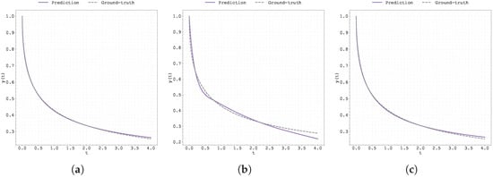
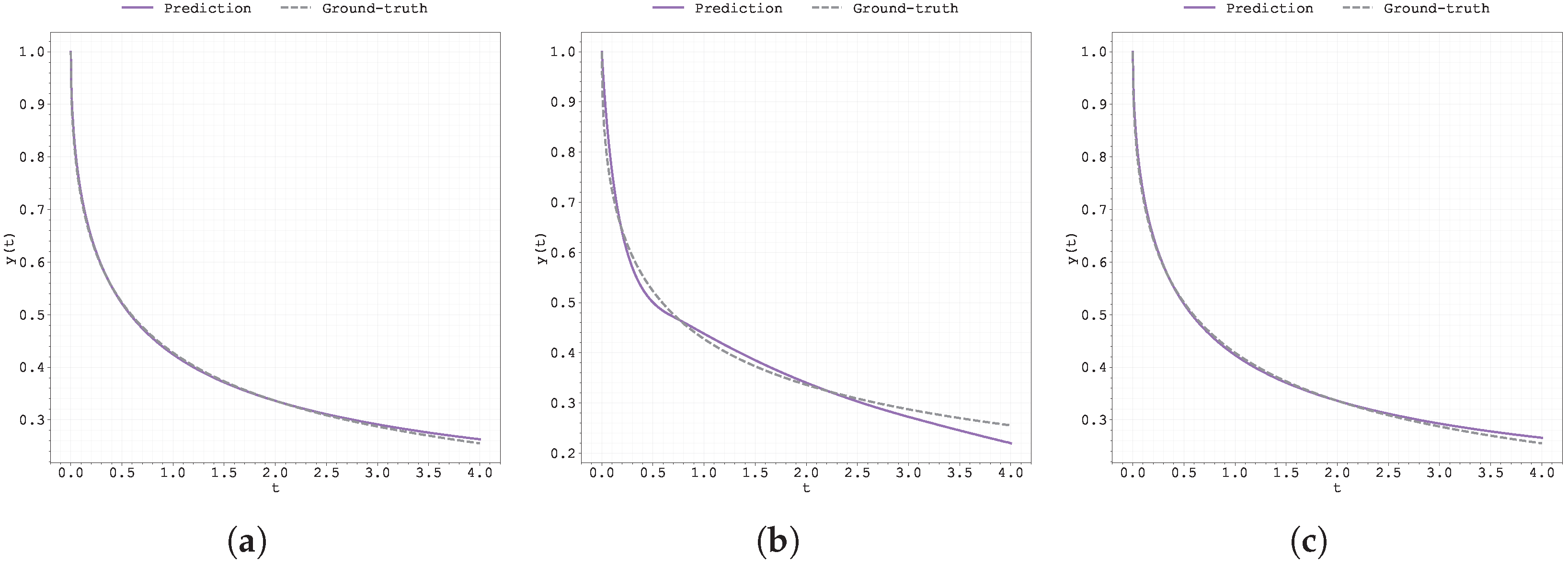
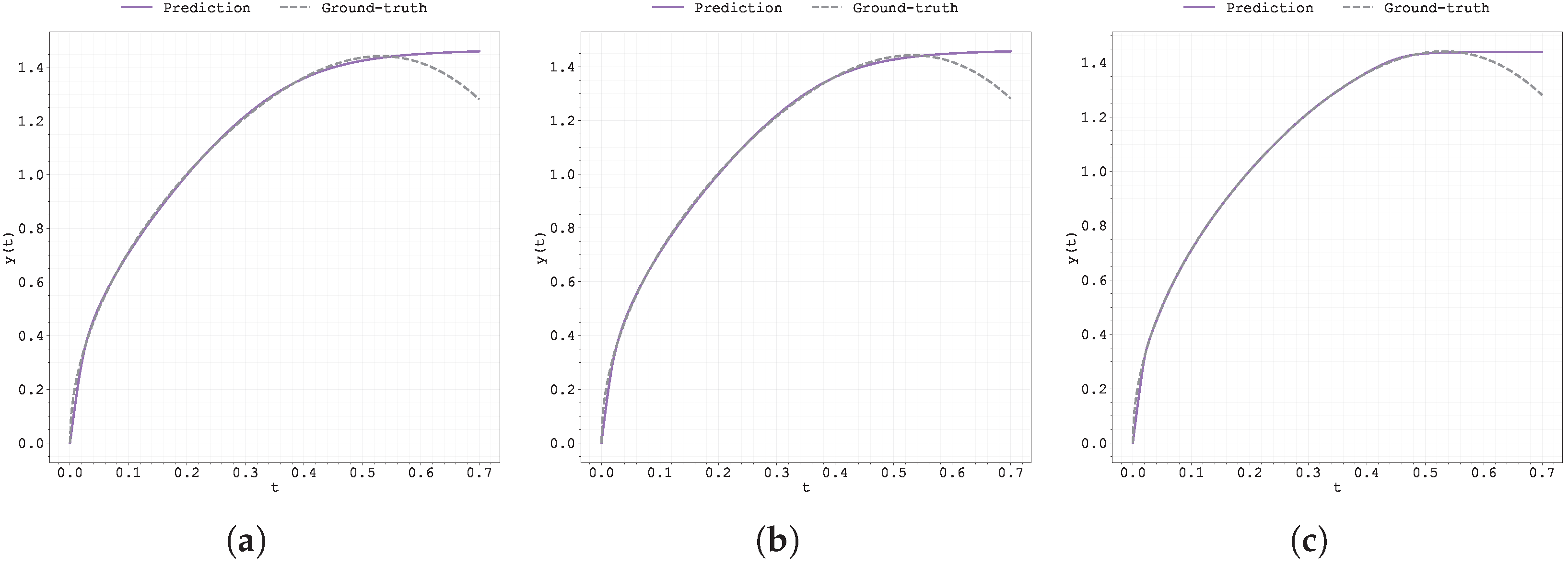
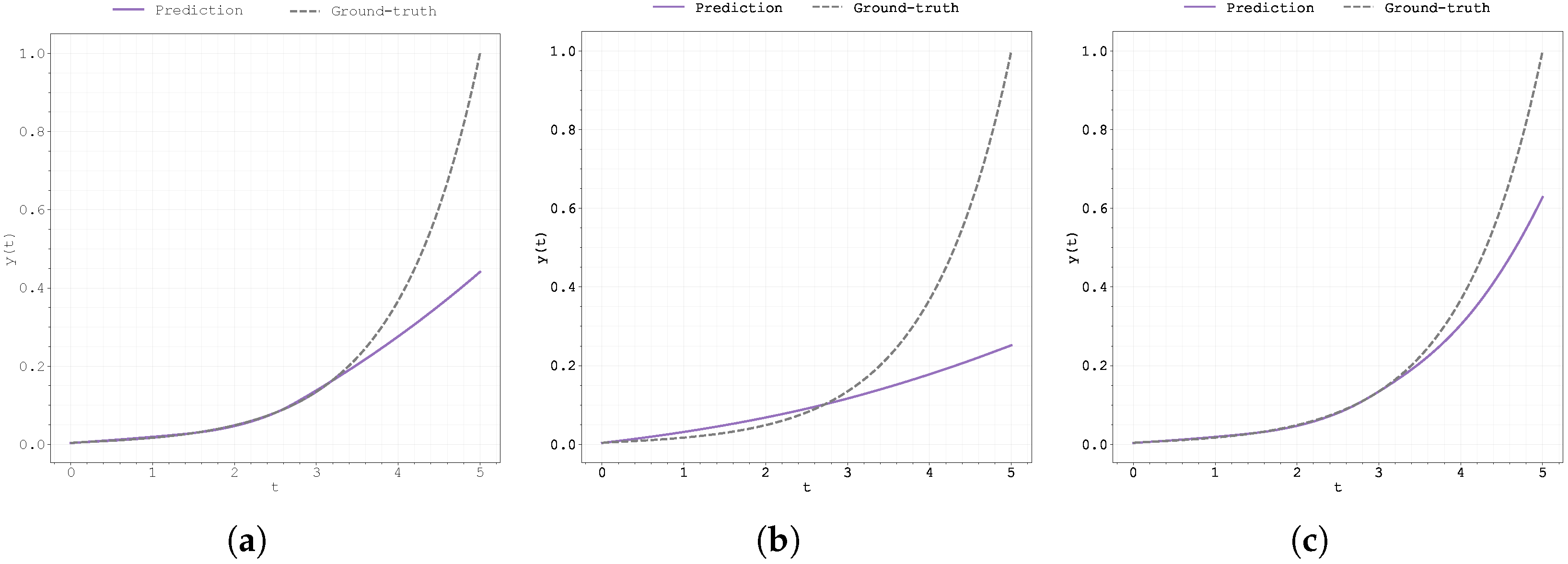
Figure 1.
Plot of the predicted and ground-truth curves from the best run in Case Study 1 with : (a) the original, (b) clipped, and (c) pre-trained Neural FDE models.
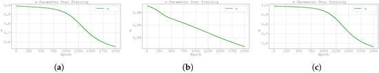
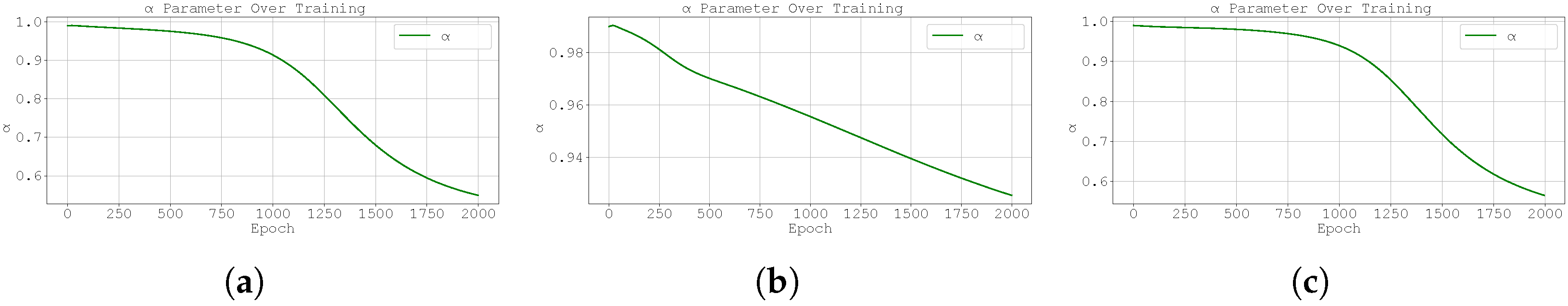
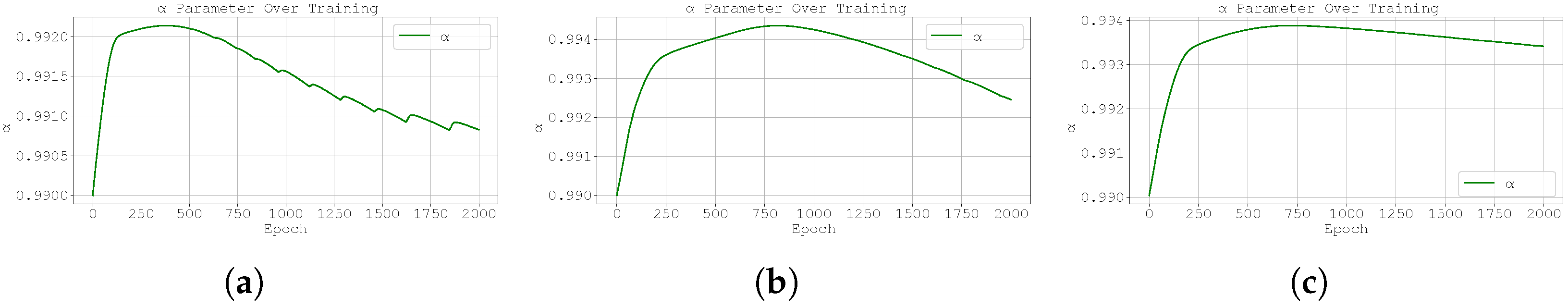
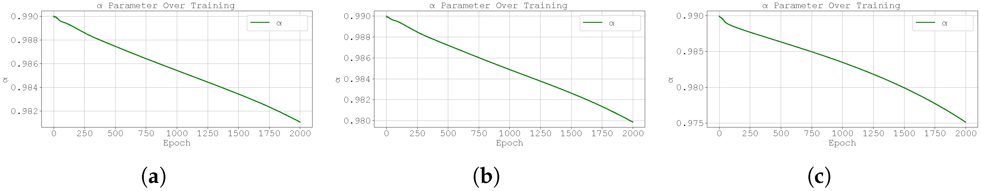
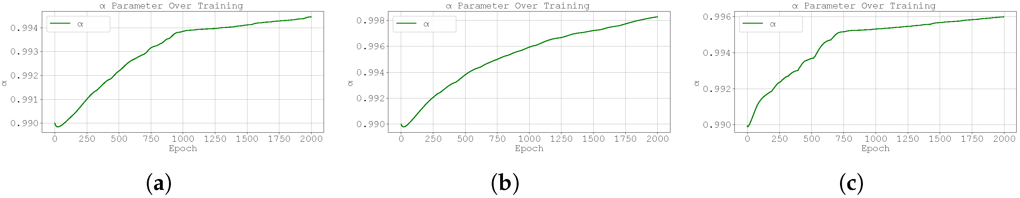
Figure 2.
Evolution of the best run’s during training for Case Study 1 with : (a) original Neural FDE, (b) clipped Neural FDE, and (c) pre-trained Neural FDE.
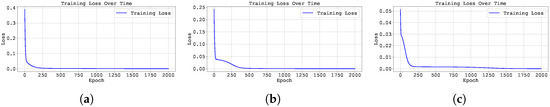
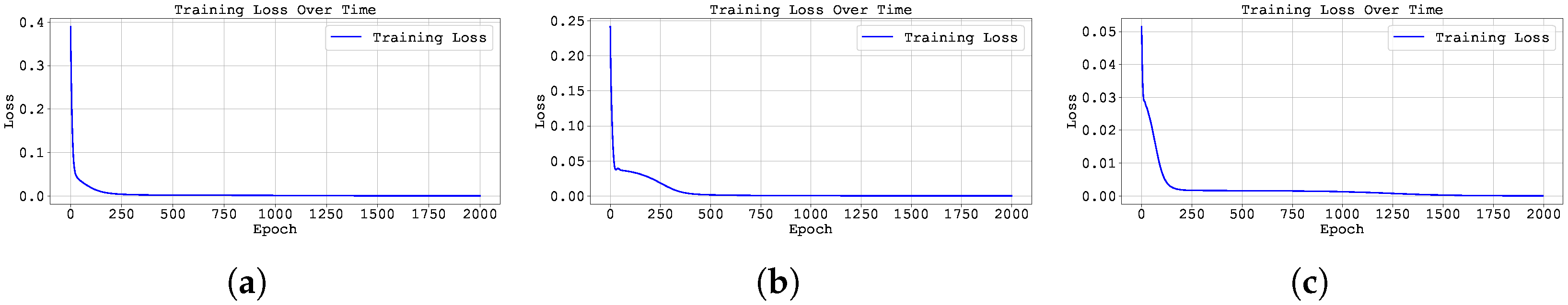
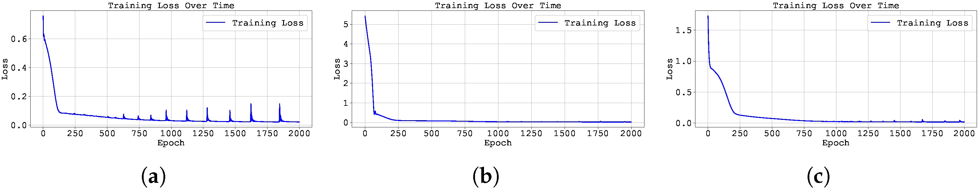
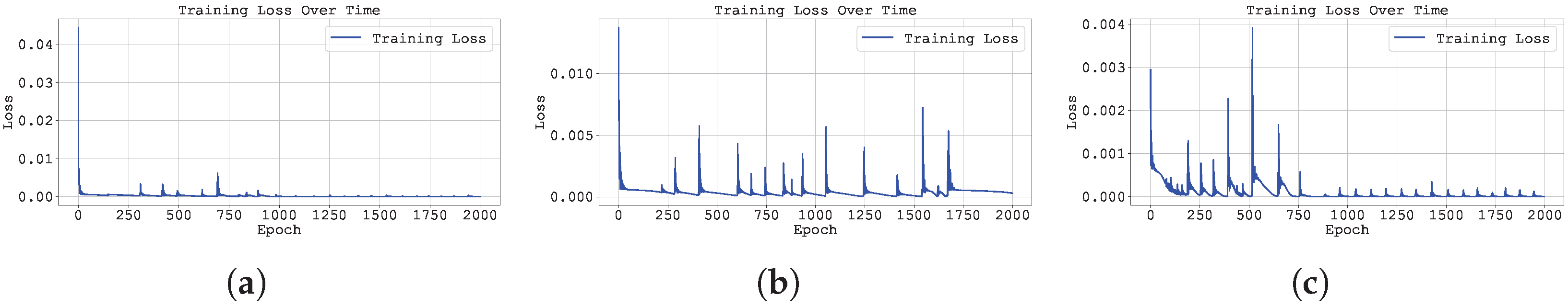
Figure 3.
Training loss across epochs for the best run in Case Study 1 with with : (a) the original, (b) clipped, and (c) pre-trained Neural FDE models.
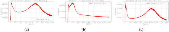
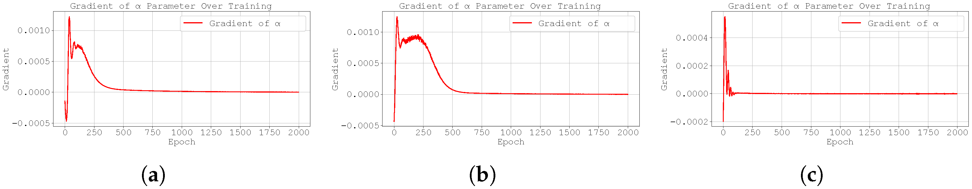
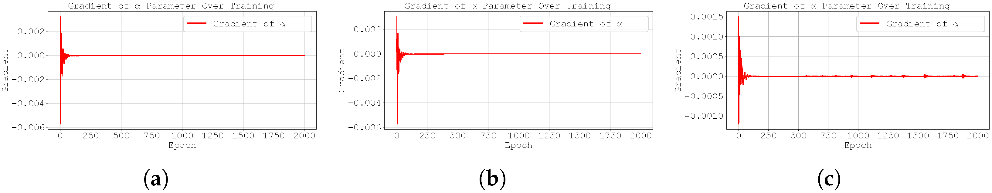
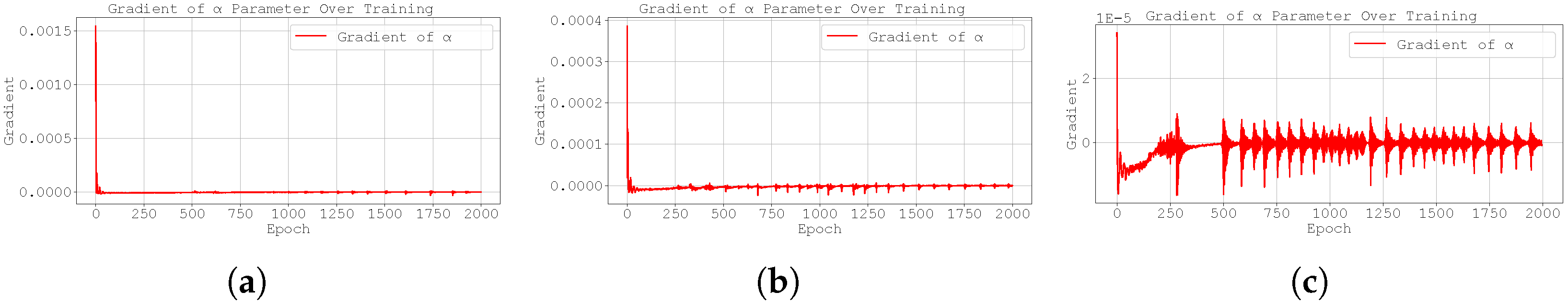
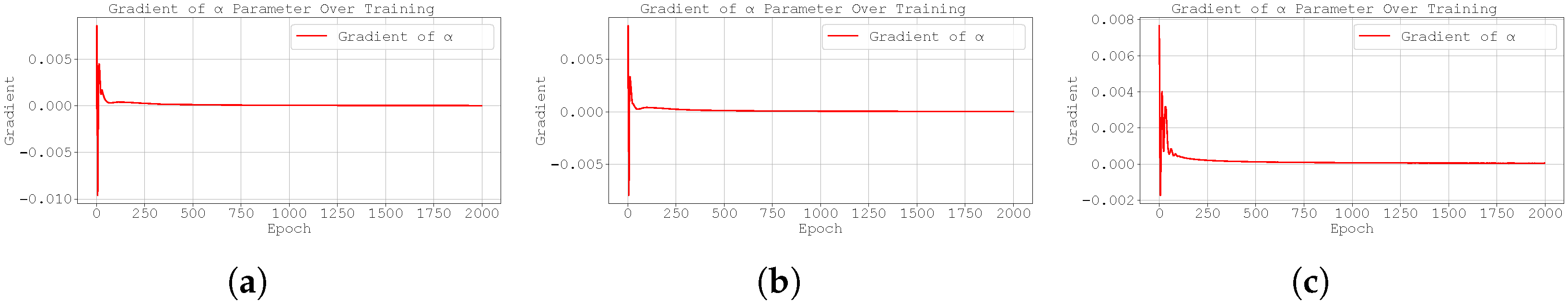
Figure 4.
Evolution of the best run’s gradient during training for Case Study 1 with with : (a) original Neural FDE, (b) clipped Neural FDE, and (c) pre-trained Neural FDE.
Table 2 (final training losses) and Table 3 (test MSE over 3 runs) confirm that, as expected, there are no significant differences in performance between the original Neural FDE method [2] and the two strategies proposed in this work.
However, Table 4 shows that while both the original Neural FDE and the pre-trained version produce predicted values of close to the ground truth, the pre-trained model significantly outperforms the original method by achieving notably more accurate estimates of , demonstrating a clear improvement in learning.
In contrast, the worst performance is observed with the gradient clipping approach, as illustrated also in Figure 1, which displays the data fitting for the case .
The good fitting performance of the original Neural FDE method (also visible in Figure 1) may be attributed to one of two reasons: either the neural network with parameters adapted effectively to the learnt value , or the discrepancy between the true value and the learnt one was not significant enough to affect the prediction quality in this particular case. The latter explanation is consistent with the sensitivity analysis discussed earlier (Table 1).
Figure 2 (evolution of during training) and Figure 3 (evolution of the loss function) indicate that gradient clipping negatively affects the update dynamics of . Specifically, the clipped- strategy appears to slow down convergence, requiring more training epochs to achieve the same level of accuracy as the other two methods.
Figure 4 shows that the gradients of the loss function with respect to are very small in this case study. This may explain why the gradient clipping technique does not yield improved results. The Adam optimiser combines momentum and adaptive learning rates by computing exponential moving averages of both the gradients and their squared values. As a result, it adjusts the step size dynamically based on the history of gradients. However, when the gradients are consistently small, the adaptive nature of Adam may result in updates that are too conservative, thereby limiting the optimiser’s ability to escape flat regions of the loss landscape or to sufficiently update . The effectiveness of the gradient clipping methodology will be better assessed in the following case studies, where larger gradients are expected to arise.
For the remaining values of , namely 0.4, 0.8 and 0.99, the results are qualitative similar to those observed for . These results are presented in Appendix A.1 to avoid cluttering of figures.
3.2. Case Study 2
Consider the following initial value problem involving a Caputo fractional derivative of order :
subject to the initial condition , where the right-hand side is given by,
The analytical solution to this problem is [26].
This particular example is noteworthy because the analytical solution does not depend on the value of , allowing the model to converge to an arbitrary fractional order. However, it is important to note that the neural network is trained to approximate the fractional derivative itself, not the solution . As such, its output inherently depends on the order . Although it is not possible to directly compute the error between the predicted and the true value of in this case, the model’s behaviour during the search for the optimal solution provides insight into how it adapts to the problem structure.
- Smoothness and Singularities: The polynomial is on withso it exhibits uniform convexity and a single turning point at . No singularities arise in y.The function is on and tends to zero as , because both exponents and are positive. Its derivatives,diverge as with orders and , respectively. Thus f has a mild slope singularity but a strong curvature singularity at the origin. On , f changes sign once and its curvature also changes sign, making f non-monotonic and non-convex overall.
The Neural FDEs considered in this case study consist of a neural network with one input layer containing a single neuron using a ReLU activation function; one hidden layer with 10 neurons and ReLU activation; and one output layer with a single neuron.
A dataset was generated from the analytical solution, with each training set comprising 500 points over the interval , and testing sets containing 700 points over . To examine the influence of the learnt and its initialisation on the Neural FDE models, we present results for two initial values of : 0.5 and 0.99.
The outcomes are summarised in Table 5, Table 6 and Table 7, while Figure 5, Figure 6, Figure 7, Figure 8, Figure 9 and Figure 10 display the training evolution of the learnt , its gradient , and the loss for both initialisations.
Table 5.
Final training loss (average MSE ± standard deviation over 3 runs) of the Neural FDE model using the three different training methods for Case Study 2.
Table 6.
Test MSE (average MSE ± standard deviation over 3 runs) of the Neural FDE using the three training methods, applied to Case Study 2.
Table 7.
Learnt values of across three runs of the Neural FDE model using the three different training methods for Case Study 2. initialised at .
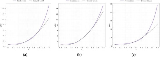
Figure 5.
Plot of the predicted and ground-truth curves from the best run in Case Study 2 with initialised at : (a) the original, (b) clipped, and (c) pre-trained Neural FDE models.
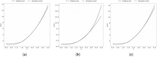
Figure 6.
Plot of the predicted and ground-truth curves from the best run in Case Study 2 with initialised at : (a) the original, (b) clipped, and (c) pre-trained Neural FDE models.
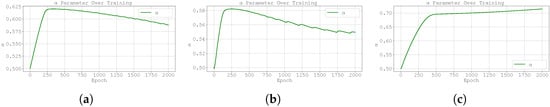
Figure 7.
Evolution of the best run’s during training for Case Study 2 with initialised at : (a) original Neural FDE, (b) clipped Neural FDE, and (c) pre-trained Neural FDE.
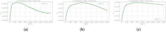
Figure 8.
Evolution of the best run’s during training for Case Study 2 with initialised at : (a) original Neural FDE, (b) clipped Neural FDE, and (c) pre-trained Neural FDE.
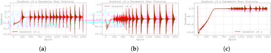
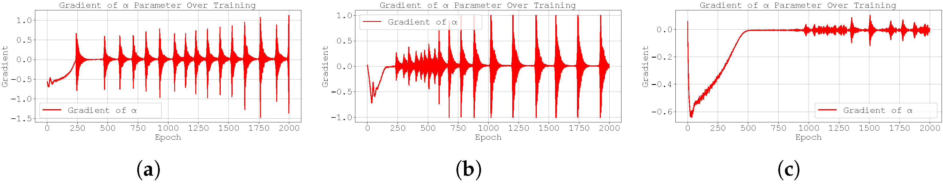
Figure 9.
Evolution of the best run’s gradient during training for Case Study 1 with initialised at : (a) original Neural FDE, (b) clipped Neural FDE, and (c) pre-trained Neural FDE.
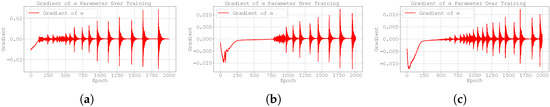
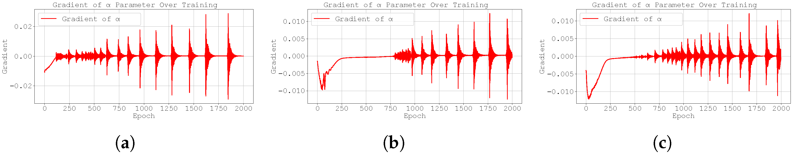
Figure 10.
Evolution of the best run’s gradient during training for Case Study 1 with initialised at : (a) original Neural FDE, (b) clipped Neural FDE, and (c) pre-trained Neural FDE.
From Table 5 and Table 6, it is evident that the initialisation of slightly influences the training performance, with an initial value of consistently yielding better results across all three methodologies. In the testing dataset, performances are comparable among the different initialisations; however, initialising at results in less consistency across training runs, as reflected by a higher standard deviation.
All three Neural FDE training approaches learn values of that remain extremely close to their initialisation value of (and ) (see Table 7 and Table 8). This indicates that, in this particular case where any should (in theory) yield a good solution (the analytical solution does not depend on ), the methodology is robust enough not to deviate significantly from the initialised .
Table 8.
Learnt values of across three runs of the Neural FDE model using the three different training methods for Case Study 2. initialised at .
Note that when is initialised at , the learnt values across the three runs exhibit greater variability (see Table 7).
Figure 5 and Figure 6 display the predicted and ground-truth curves from the best runs in Case Study 2, with initialised at 0.5 and 0.99, respectively. For the case , the pre-trained methodology appears to deviate from the ground truth in the testing region; however, overall, this approach delivers the best results.
During training (Figure 7, where ), the parameter exhibits a sharp increase for both the original and gradient-clipped Neural FDEs. A similar trend is observed when , although in this case, the clipped model displays a smoother evolution compared to the scenario with (Figure 8).
Furthermore, both the original and clipped models show significant oscillations in the gradient throughout training. While the pre-trained Neural FDE exhibits similar behaviour, the oscillations are noticeably more stable, suggesting that the pre-training phase contributes to a more robust and consistent learning process (see Figure 9 and Figure 10).
It is also worth noting that the amplitude of the oscillations is substantially larger in the case where (the scales used in Figure 9 and Figure 10 are different). For values of closer to 1, the right-hand-side function becomes smoother and, in principle, easier to learn. As a result, the optimisation process may tend to favour higher values of within the range .
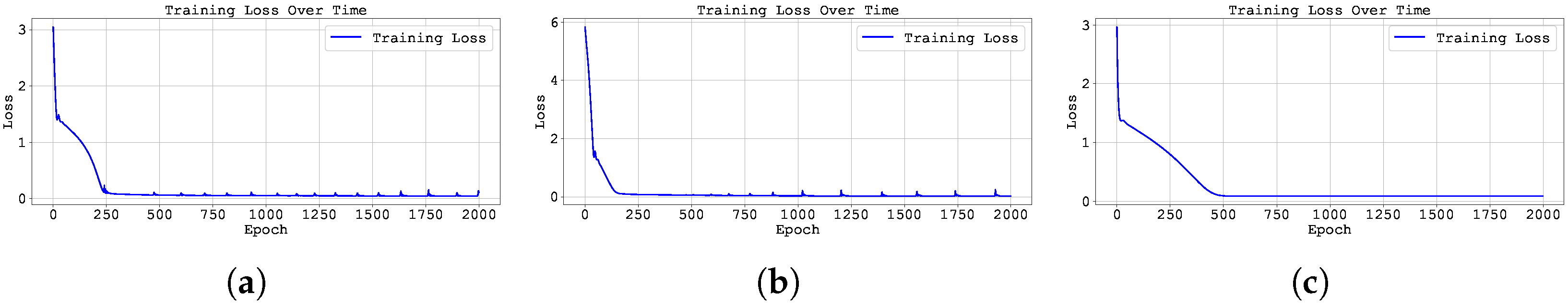
These oscillations are reflected in the behaviour of the loss function. Figure 11 and Figure 12 show that the pre-training method exhibits a smoother evolution of the loss compared to the other two approaches.
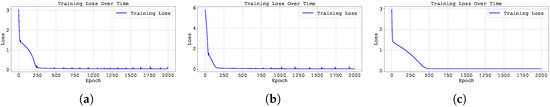
Figure 11.
Training loss across epochs for the best run in Case Study 2 with initialised at : (a) the original, (b) clipped, and (c) pre-trained Neural FDE models.
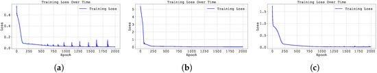
Figure 12.
Training loss across epochs for the best run in Case Study 2 with initialised at : (a) the original, (b) clipped, and (c) pre-trained Neural FDE models.
3.3. Case Study 3
Consider the following initial value problem involving the Caputo fractional derivative of order :
subject to the initial condition , where the right-hand side is defined as,
We consider the interval , for which the analytical solution is given by
as established in [9]. In this case, the analytical solution includes a term of the form , which introduces a more pronounced non-smoothness to the solution.
We compare the solution for with a perturbed order . Table 9 shows the values of for both cases and the absolute differences , at selected time points.
Table 9.
Comparison between the solutions and right-hand-side terms of the fractional ODE for and .
Varying induces small changes in both the solution and the right-hand-side function. However, these variations are slightly more pronounced than those observed in Case Study 1.
- Smoothness and Singularities:Near , the term in and in dominate, producing a weak slope singularity of order and a strong curvature singularity of order . As t increases, the high-degree monomials and prevail, introducing inflection points and reversals of concavity.The function is a sum of fractional powers and highly nonlinear terms. Its first and second derivatives consist of sums of powers , where near the most singular exponent arises from differentiating . One finds curvature singularities of order up to , which can be exceptionally strong if is small. Throughout , f exhibits multiple sign changes, several inflection points, and rapid oscillations of curvature, reflecting high analytical complexity.
For this case study, four datasets were generated corresponding to different values of the fractional order, namely , , and . The training set consists of 300 data points uniformly distributed over the interval , while the testing set includes 400 points in the extended range .
The Neural FDE models employ a neural network with the following architecture: one input layer with a single neuron using a tanh activation function; two hidden layers with 128 neurons each—where the first uses the exponential linear unit (ELU) activation and the second uses tanh; and a final output layer with one neuron. The fractional order was initialised at . In this case, a more robust neural network was considered in order to deal the characteristics of the problem at hands.
The corresponding results are presented in Table 10, Table 11 and Table 12. Figure 13, Figure 14, Figure 15 and Figure 16 illustrate the training dynamics for the case , including the evolution of the learnt order , its gradient , and the loss function. Additional results for and are provided in Appendix A.2, in Figure A13, Figure A14, Figure A15, Figure A16, Figure A17, Figure A18, Figure A19 and Figure A20.
Table 10.
Final training loss (average MSE ± standard deviation over 3 runs) of the Neural FDE model using the three different training methods for Case Study 3.
Table 11.
Test MSE (average MSE ± standard deviation over 3 runs) of the Neural FDE using the three training methods, applied to Case Study 3.
Table 12.
Learnt values of across three runs of the Neural FDE model using the three different training methods for Case Study 3. Results are reported as the mean MSE ± standard deviation.
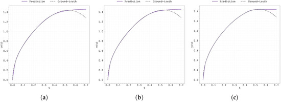
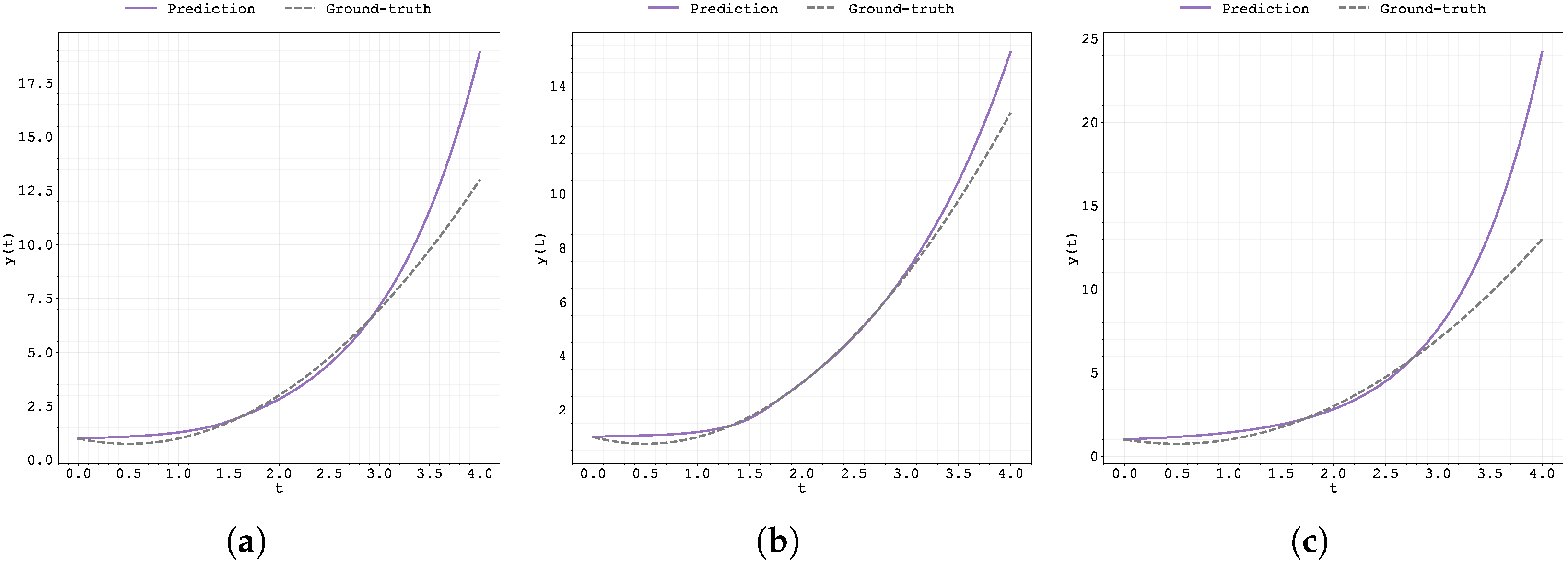
Figure 13.
Plot of the predicted and ground-truth curves from the best run in Case Study 3 with : (a) the original, (b) clipped, and (c) pre-trained Neural FDE models.
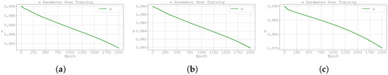
Figure 14.
Evolution of the best run’s during training for Case Study 3 with : (a) original Neural FDE, (b) clipped Neural FDE, and (c) pre-trained Neural FDE.
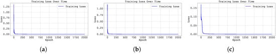
Figure 15.
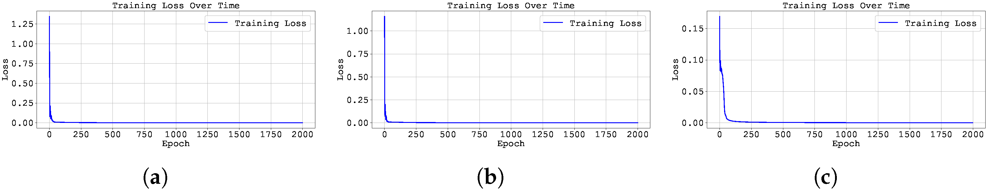
Training loss across epochs for the best run in Case Study 3 with : (a) the original, (b) clipped, and (c) pre-trained Neural FDE models.
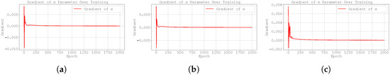
Figure 16.
Evolution of the best run’s gradient during training for Case Study 3 with : (a) original Neural FDE, (b) clipped Neural FDE, and (c) pre-trained Neural FDE.
From Table 10 and Table 11, all three methodologies have similar training and testing performance. Furthermore, the learnt of all three methodologies are similar, close to 0.99, independently of the ground-truth value of the dataset being modelled. These results highlight the difficulty the model faces in accurately learning the correct value of using any of the methods. The loss function consistently favours values of close to 1 (even when considering different initialisations of ).
Remark:
It should be noted, however, that increasing the number of training epochs leads to a gradual decrease in the value of towards its expected value. Nevertheless, the convergence rate is so slow that the associated computation times become prohibitively high, rendering this approach inefficient in practice.
From Figure 13, Figure 14, Figure 15, Figure 16, Figure 17, Figure 18, Figure 19, Figure 20, Figure A1, Figure A2, Figure A3, Figure A4, Figure A5, Figure A6, Figure A7, Figure A8, Figure A9, Figure A10, Figure A11, Figure A12, Figure A13, Figure A14, Figure A15, Figure A16, Figure A17, Figure A18, Figure A19 and Figure A20, unlike in the previous case study, both the loss and the gradient with respect to remain stable throughout training. However, when analysing the prediction curves (Figure 13, Figure A13 and Figure A17), it becomes clear that although the models fit the data well up to , they struggle to generalise beyond that point.
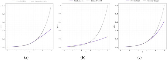
Figure 17.
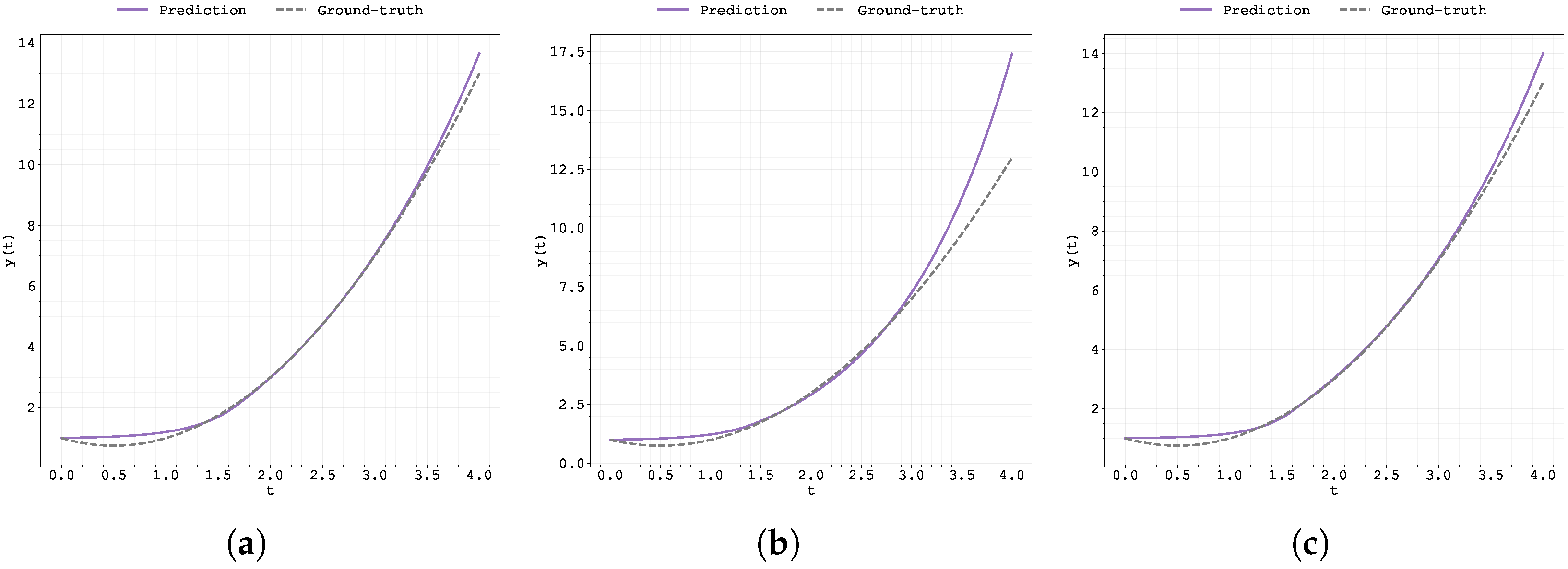
Plot of the predicted and ground-truth curves from the best run in Case Study 4 with : (a) the original, (b) clipped, and (c) pre-trained Neural FDE models.
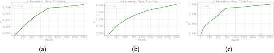
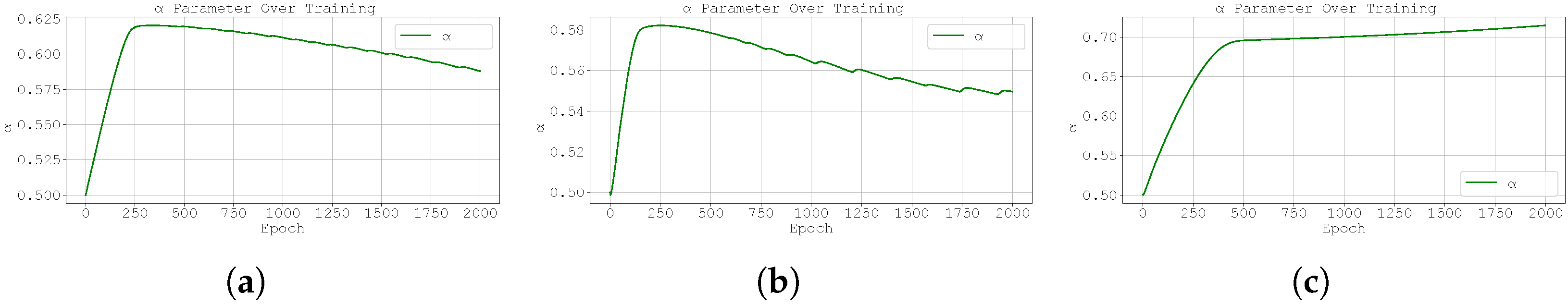
Figure 18.
Evolution of the best run’s during training for Case Study 4 with : (a) original Neural FDE, (b) clipped Neural FDE, and (c) pre-trained Neural FDE.
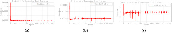
Figure 19.
Plot of the best run gradient value through training for Case Study 4, with : (a) original, (b) clipped and (c) pre-trained Neural FDE.
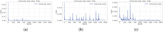
Figure 20.
Training loss across epochs for the best run in Case Study 4 with : (a) the original, (b) clipped, and (c) pre-trained Neural FDE models.
This weaker performance in the latter part of the time interval is likely due to a shift in the underlying dynamics, which were not present in the training data. For the models to successfully extrapolate, additional training data in the interval would be necessary.
3.4. Case Study 4
Consider again the initial value problem:
but now with . We compare the solution () for with a perturbed order . Table 13 shows the values of for both cases and the absolute difference at selected time points:
Table 13.
Comparison between the solutions of problem (11), with , for the fractional orders and .
For , we observe that:
This difference satisfies the inequality
where , which implies that 32,392.
Such a large value of K highlights the strong sensitivity of the solution with respect to small perturbations in the fractional order , particularly for large t. This indicates that the problem may exhibit a not so well-posed behaviour, where small variations in the problem data result in substantial changes in the solution (or right-hand-side function).
- Smoothness and Singularities: Similar to Case Study 1. Both and diverge with orders and . For , all derivatives exist and remain positive, so y grows monotonically and stays strictly convex (no inflection). The right-hand side shares these properties exactly.
Using the analytical solution, four datasets were generated for , , and . Each dataset contains 1500 points in the interval for training and 1500 points in the interval for testing. The Neural FDE models use a neural network with the following architecture: one input layer with a single neuron and a hyperbolic tangent (tanh) activation function; two hidden layers with 64 neurons each and ReLU activations; and one output layer with a single neuron. The fractional order was initialised at for all experiments.
The corresponding results are summarised in Table 14, Table 15 and Table 16. The evolution of the learnt order , its gradient , and the training loss are depicted in Figure 17, Figure 18, Figure 19 and Figure 20 for , and in Appendix A.3, Figure A21, Figure A22, Figure A23, Figure A24, Figure A25, Figure A26, Figure A27 and Figure A28, for and .
Table 14.
Final training loss (average MSE ± standard deviation over 3 runs) of the Neural FDE model using the three different training methods for Case Study 4.
Table 15.
Test MSE (average MSE ± standard deviation over 3 runs) of the Neural FDE using the three training methods, applied to Case Study 4.
Table 16.
Learnt values of across three runs of the Neural FDE model using the three different training methods for Case Study 4. Results are reported as the mean MSE ± standard deviation.
The results presented in Table 14, Table 15 and Table 16 indicate that all three methodologies exhibit similar performance in terms of fitting the data and predicting the solution’s evolution. However, as shown in Figure 18, the best results for the most successful run were achieved using the pre-trained methodology.
It is worth noting that the clipped methodology produced very poor results, despite achieving a low final training loss. This discrepancy suggests a potential issue or instability with the training process that may depend on the initialisations used.
Once again, the model failed to accurately learn the correct order of the derivative. In all cases, the optimal value of converged to approximately 1, regardless of the true value used during training (see also Figure 18). Furthermore, the gradient of exhibited large-amplitude oscillations when using the pre-trained method, suggesting that this approach struggles to handle the irregular behaviour observed in this particular case study (see Table 13).
4. Conclusions
This work presents a fundamental study of two methodologies for the joint optimisation of the fractional derivative order and the parameters of the right-hand-side neural network in Neural FDE models. One approach involves bounding the gradient magnitude of the loss function with respect to , promoting more stable and effective updates. Another strategy introduces an online pre-training scheme, in which the network parameters are first optimised over progressively longer time intervals, while is updated more conservatively using the full time trajectory.
Several case studies were analysed, encompassing problems where the analytical solution and the right-hand-side function exhibit different levels of regularity and varying degrees of dependence on data.
In every case the solution and the forcing are on the open interval, but typically admit a weak slope singularity of order and a stronger curvature singularity of order (or worse) at . The quadratic case (Study 2) is the only example without singularities in y itself; all others exhibit algebraic bends near the origin whose strength and complexity depend on the lowest fractional exponent. The curvature profiles range from simple constant concavity (Study 2) to multiple inflections and high nonlinearity (Study 3).
In scenarios with mildly smooth solutions, the proposed methodologies successfully converged to values of that approximate the ground truth. In cases where the solution itself does not depend on , but the right-hand-side function does, the optimisation algorithm was able to maintain the initial value of , without drifting unnecessarily.
The final two case studies demonstrated the limitations of the proposed methods. In Case Study 3, convergence to the correct fractional order was not achieved within a practical number of epochs, although it is likely that significantly increasing the training time could improve results. In the last case study, small perturbations in the fractional order caused large variations in the right-hand-side function. As a result, despite a good fit to the data, the optimisation algorithm consistently drifted towards (even for different initialisations of ).
This work aims to encourage further developments towards methods that not only achieve a good fit to data (a goal successfully attained in the present study) but also ensure convergence to the ground-truth order of the derivative. While the proposed approaches demonstrate promising results in favourable scenarios, they fall short in more challenging problems, particularly those involving low regularity or high sensitivity to the fractional order. These limitations highlight the need for more robust optimisation strategies capable of addressing such complexities.
While our experiments demonstrate the efficacy of Neural FDEs, fractional derivatives are indeed known to enhance the modelling of periodic and chaotic dynamics in nonlinear systems. For instance, fractional-order variants of the Lorenz and Rössler systems exhibit rich bifurcation behaviours and chaotic attractors, while fractional extensions of the KdV and nonlinear Schrödinger equations support soliton solutions with anomalous dispersion [27,28,29,30]. Although such cases are beyond the scope of this work, our framework is theoretically compatible with these systems, as it learns the fractional dynamics directly from data without presuming a specific structure. Future research will explore Neural FDEs for chaotic systems and soliton dynamics, where the non-local memory effects of fractional derivatives could prove particularly advantageous.
Author Contributions
Conceptualisation, C.C., M.F.P.C. and L.L.F.; methodology, C.C., M.F.P.C. and L.L.F.; software, C.C.; validation, C.C. and L.L.F.; formal analysis, C.C. and L.L.F.; investigation, C.C. and L.L.F.; resources, C.C. and L.L.F.; data curation, C.C. and L.L.F.; writing—original draft preparation, C.C. and L.L.F.; writing—review and editing, C.C., M.F.P.C. and L.L.F.; visualisation, C.C.; supervision, M.F.P.C., O.N. and L.L.F.; project administration, O.N. and L.L.F.; funding acquisition, C.C., O.N. and L.L.F. All authors have read and agreed to the published version of the manuscript.
Funding
The authors acknowledge funding by Fundação para a Ciência e Tecnologia (Portuguese Foundation for Science and Technology) through CMAT projects UIDB/00013/2020 and the support of the High-Performance Computing Center at the University of Évora funded by FCT I.P. under the project “OptXAI: Constrained optimisation in NNs for Explainable, Ethical and Greener AI”, reference 2024.00191.CPCA.A1, platform Vision. C. Coelho would like to thank the KIBIDZ project funded by dtec.bw—Digitalization and Technology Research Center of the Bundeswehr; dtec.bw is funded by the European Union—NextGenerationEU. This work was also financially supported by national funds through the FCT/MCTES (PIDDAC) under the project 2022.06672.PTDC—iMAD (Improving the Modelling of Anomalous Diffusion and Viscoelasticity: solutions to industrial problems), DOI 10.54499/2022.06672.PTDC (https://doi.org/10.54499/2022.06672.PTDC); and by the projects LA/P/0045/2020 (ALiCE), UIDB/00532/2020, and UIDP/00532/2020 (CEFT). It was also financially supported by Fundação “la Caixa”|BPI and FCT through project PL24-00057: “Inteligência Artificial na Otimização da Rega para Olivais Resilientes às Alterações Climáticas”.
Data Availability Statement
The original contributions presented in this study are included in the article. Further inquiries can be directed to the corresponding author.
Conflicts of Interest
The authors declare no conflicts of interest.
Appendix A. Additional Plots
Appendix A.1. Case Study 1
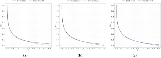
Figure A1.
Plot of the predicted and ground-truth curves from the best run in Case Study 1 with initialised at : (a) the original, (b) clipped, and (c) pre-trained Neural FDE models.
Figure A1.
Plot of the predicted and ground-truth curves from the best run in Case Study 1 with initialised at : (a) the original, (b) clipped, and (c) pre-trained Neural FDE models.
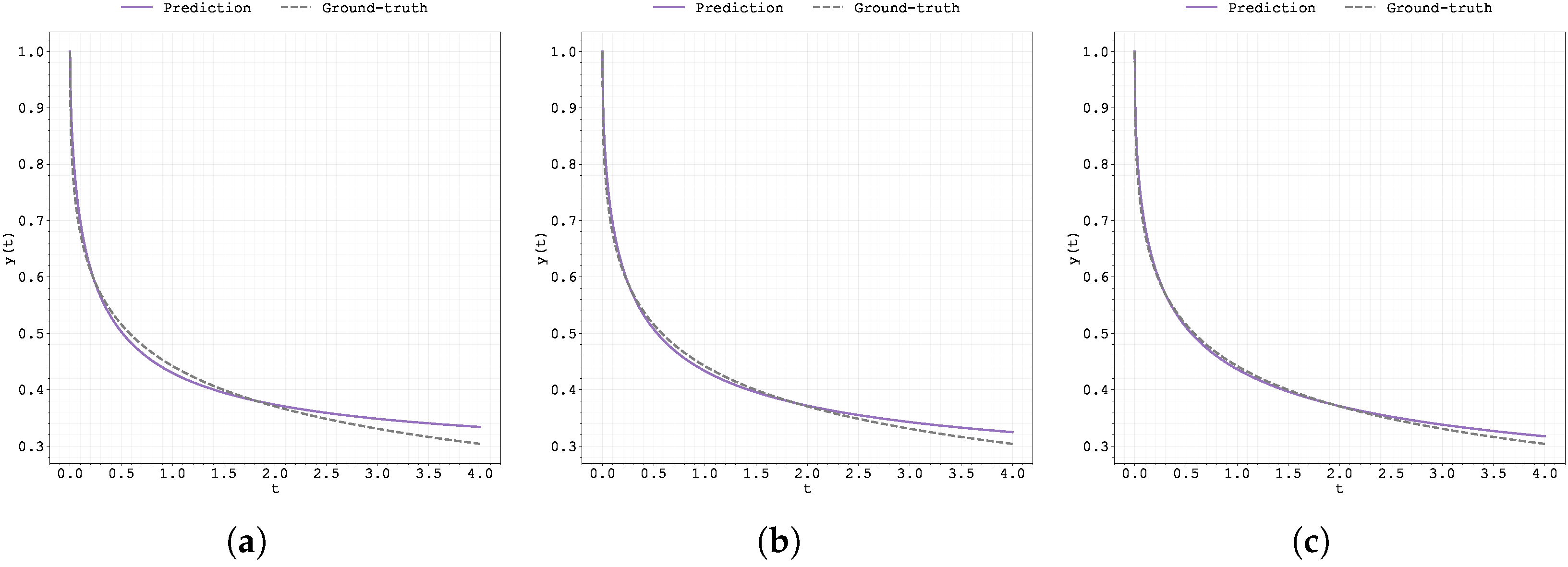
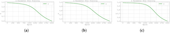
Figure A2.
Evolution of the best run’s during training for Case Study 1 with : (a) original Neural FDE, (b) clipped Neural FDE, and (c) pre-trained Neural FDE.
Figure A2.
Evolution of the best run’s during training for Case Study 1 with : (a) original Neural FDE, (b) clipped Neural FDE, and (c) pre-trained Neural FDE.
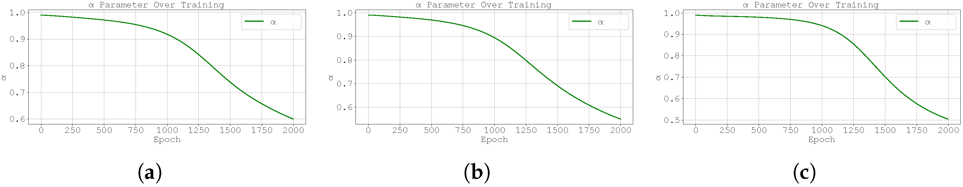
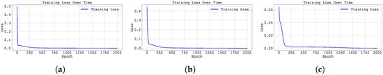
Figure A3.
Training loss across epochs for the best run in Case Study 1 with : (a) the original, (b) clipped, and (c) pre-trained Neural FDE models.
Figure A3.
Training loss across epochs for the best run in Case Study 1 with : (a) the original, (b) clipped, and (c) pre-trained Neural FDE models.
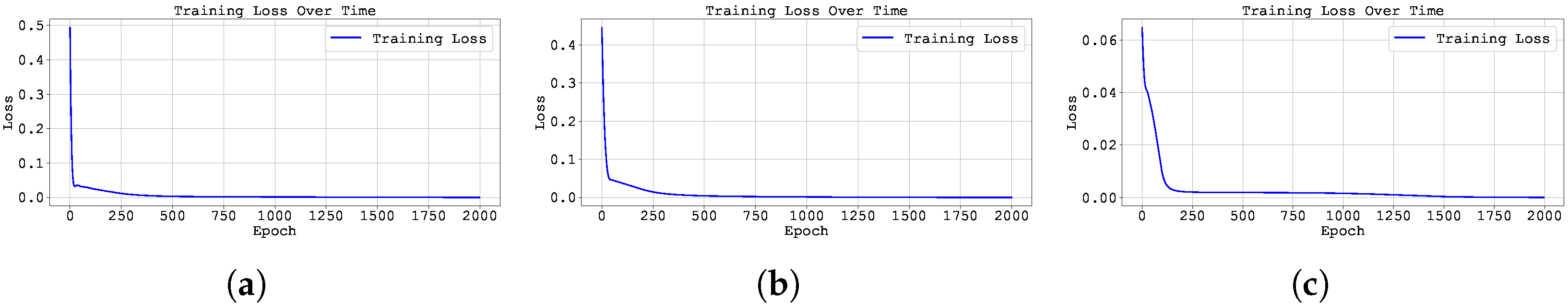
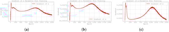
Figure A4.
Plot of the best run gradient value through training for Case Study 1, with , for (a) original, (b) clipped and (c) pre-trained Neural FDE.
Figure A4.
Plot of the best run gradient value through training for Case Study 1, with , for (a) original, (b) clipped and (c) pre-trained Neural FDE.

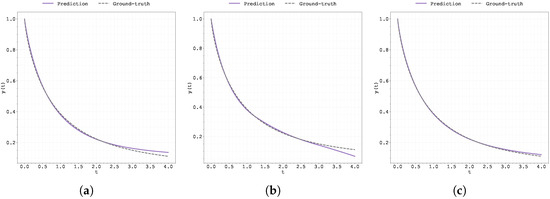
Figure A5.
Plot of the predicted and ground-truth curves from the best run in Case Study 1 with initialised at : (a) the original, (b) clipped, and (c) pre-trained Neural FDE models.
Figure A5.
Plot of the predicted and ground-truth curves from the best run in Case Study 1 with initialised at : (a) the original, (b) clipped, and (c) pre-trained Neural FDE models.
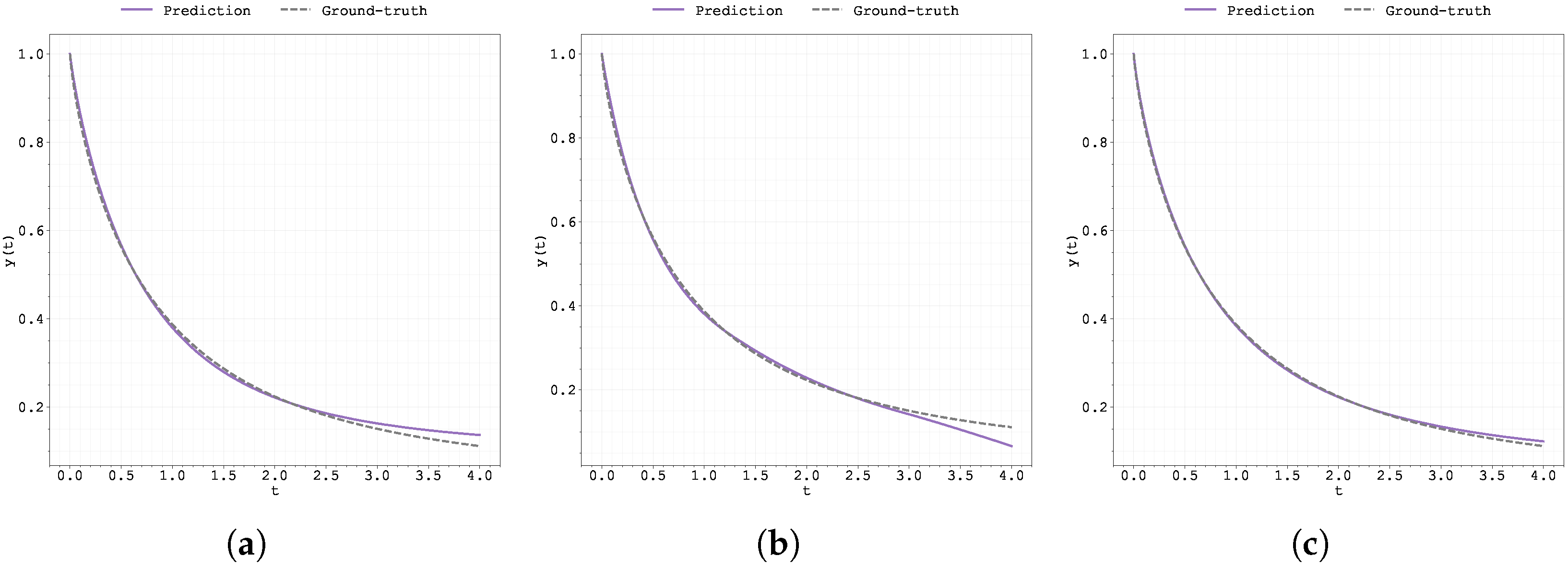
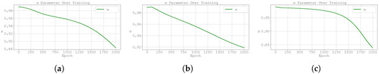
Figure A6.
Evolution of the best run’s during training for Case Study 1 with : (a) original Neural FDE, (b) clipped Neural FDE, and (c) pre-trained Neural FDE.
Figure A6.
Evolution of the best run’s during training for Case Study 1 with : (a) original Neural FDE, (b) clipped Neural FDE, and (c) pre-trained Neural FDE.
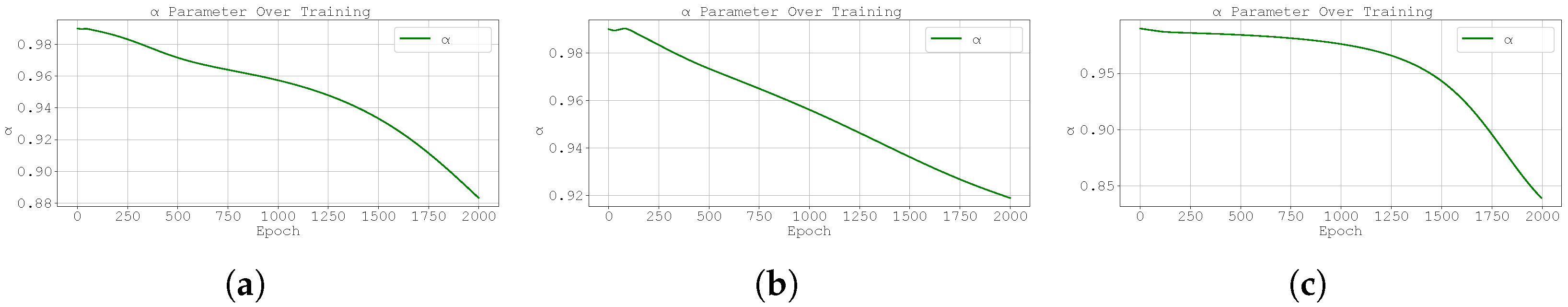
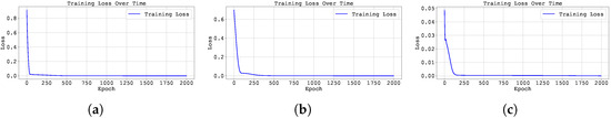
Figure A7.
Training loss across epochs for the best run in Case Study 1 with : (a) the original, (b) clipped, and (c) pre-trained Neural FDE models.
Figure A7.
Training loss across epochs for the best run in Case Study 1 with : (a) the original, (b) clipped, and (c) pre-trained Neural FDE models.
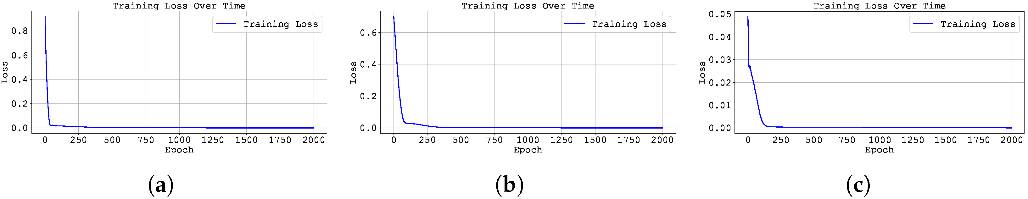
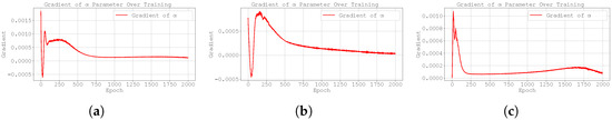
Figure A8.
Plot of the best run gradient value through training for Case Study 1, with , for (a) original, (b) clipped and (c) pre-trained Neural FDE.
Figure A8.
Plot of the best run gradient value through training for Case Study 1, with , for (a) original, (b) clipped and (c) pre-trained Neural FDE.
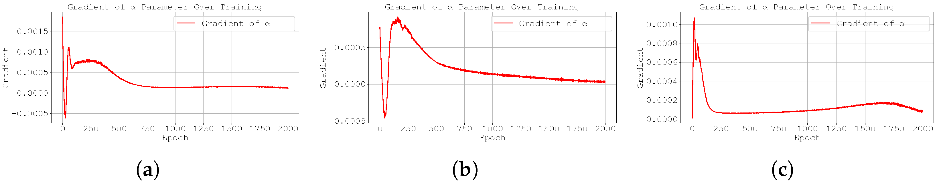
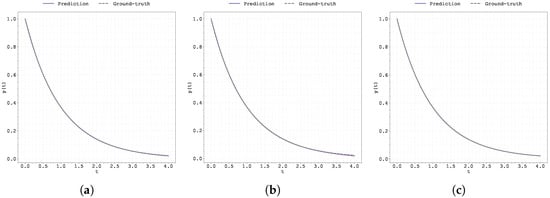
Figure A9.
Plot of the predicted and ground-truth curves from the best run in Case Study 1 with initialised at : (a) the original, (b) clipped, and (c) pre-trained Neural FDE models.
Figure A9.
Plot of the predicted and ground-truth curves from the best run in Case Study 1 with initialised at : (a) the original, (b) clipped, and (c) pre-trained Neural FDE models.

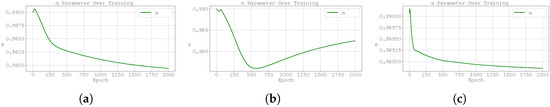
Figure A10.
Evolution of the best run’s during training for Case Study 1 with : (a) original Neural FDE, (b) clipped Neural FDE, and (c) pre-trained Neural FDE.
Figure A10.
Evolution of the best run’s during training for Case Study 1 with : (a) original Neural FDE, (b) clipped Neural FDE, and (c) pre-trained Neural FDE.
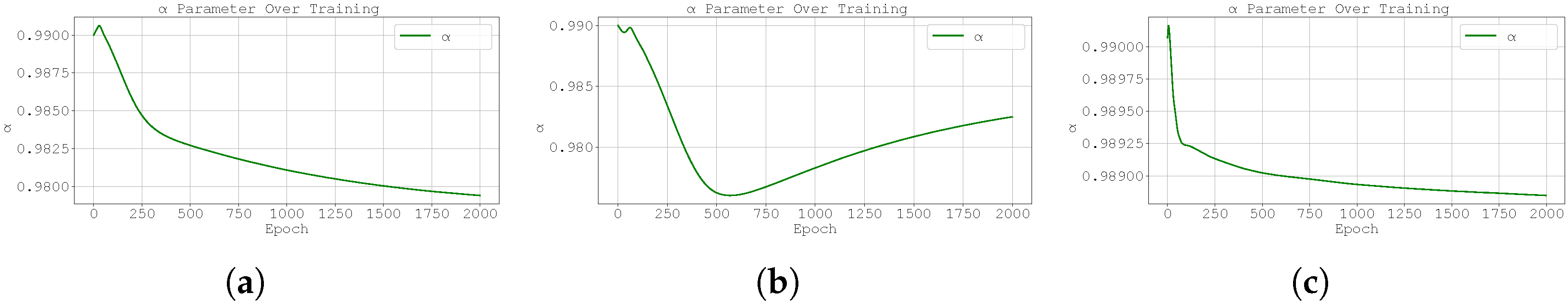
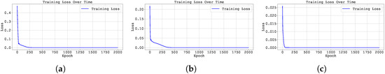
Figure A11.
Training loss across epochs for the best run in Case Study 1 with : (a) the original, (b) clipped, and (c) pre-trained Neural FDE models.
Figure A11.
Training loss across epochs for the best run in Case Study 1 with : (a) the original, (b) clipped, and (c) pre-trained Neural FDE models.
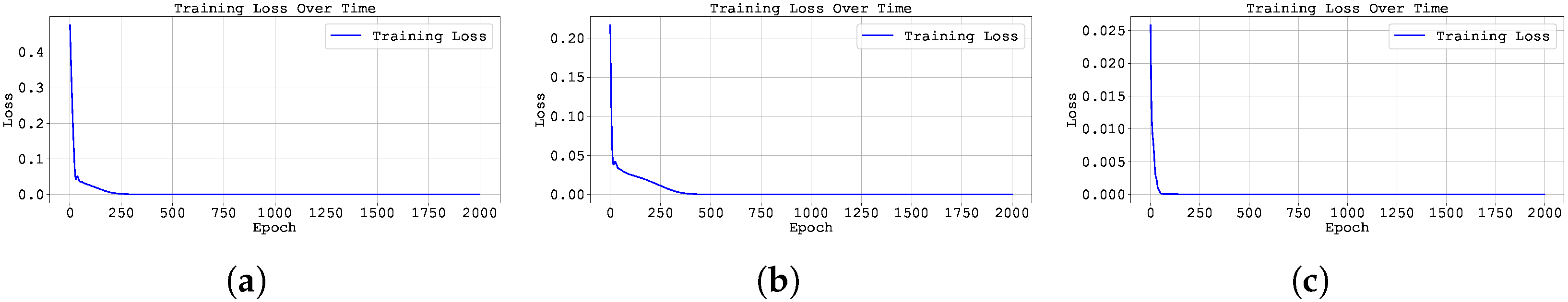
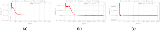
Figure A12.
Plot of the best run gradient value through training for Case Study 1, with , for (a) original, (b) clipped and (c) pre-trained Neural FDE.
Figure A12.
Plot of the best run gradient value through training for Case Study 1, with , for (a) original, (b) clipped and (c) pre-trained Neural FDE.
Appendix A.2. Case Study 3
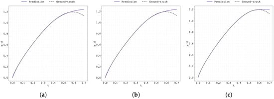
Figure A13.
Plot of the predicted and ground-truth curves from the best run in Case Study 3 with initialised at : (a) the original, (b) clipped, and (c) pre-trained Neural FDE models.
Figure A13.
Plot of the predicted and ground-truth curves from the best run in Case Study 3 with initialised at : (a) the original, (b) clipped, and (c) pre-trained Neural FDE models.
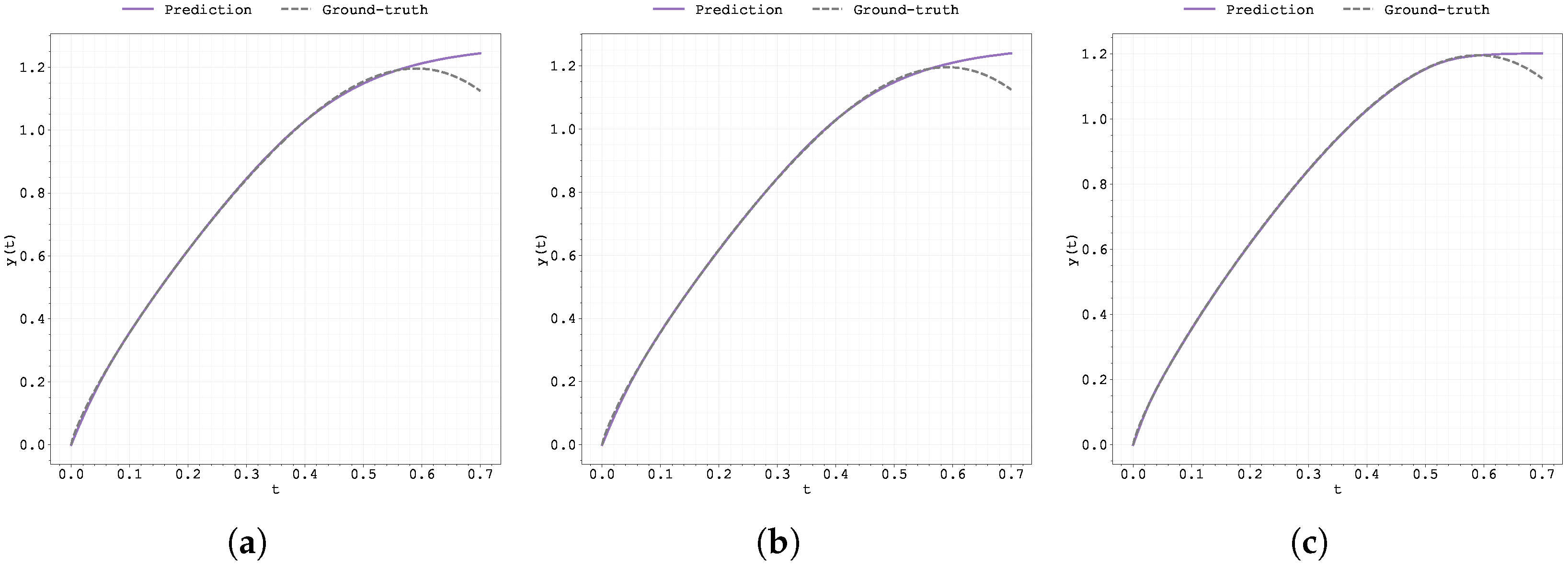
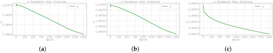
Figure A14.
Evolution of the best run’s during training for Case Study 3 with : (a) original Neural FDE, (b) clipped Neural FDE, and (c) pre-trained Neural FDE.
Figure A14.
Evolution of the best run’s during training for Case Study 3 with : (a) original Neural FDE, (b) clipped Neural FDE, and (c) pre-trained Neural FDE.
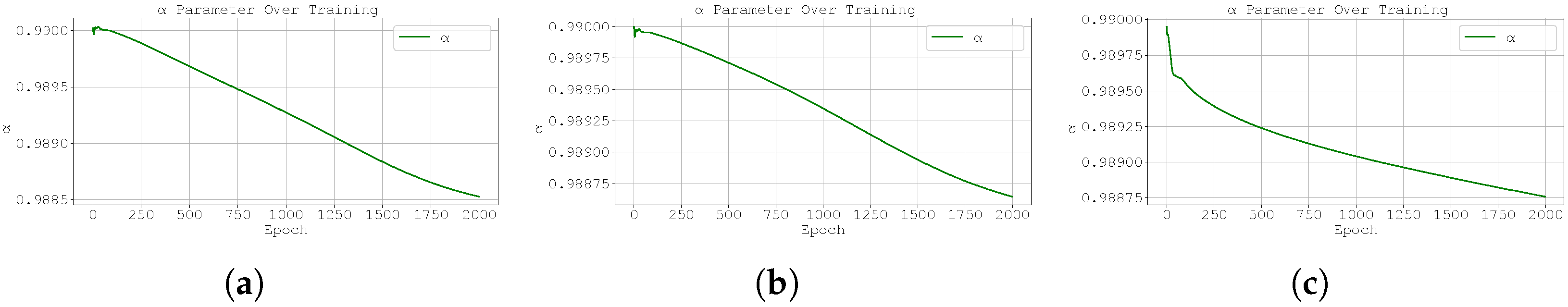
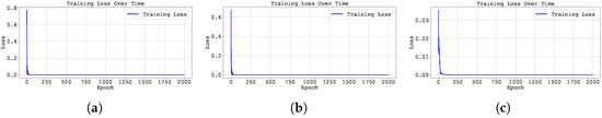
Figure A15.
Training loss across epochs for the best run in Case Study 3 with : (a) the original, (b) clipped, and (c) pre-trained Neural FDE models.
Figure A15.
Training loss across epochs for the best run in Case Study 3 with : (a) the original, (b) clipped, and (c) pre-trained Neural FDE models.
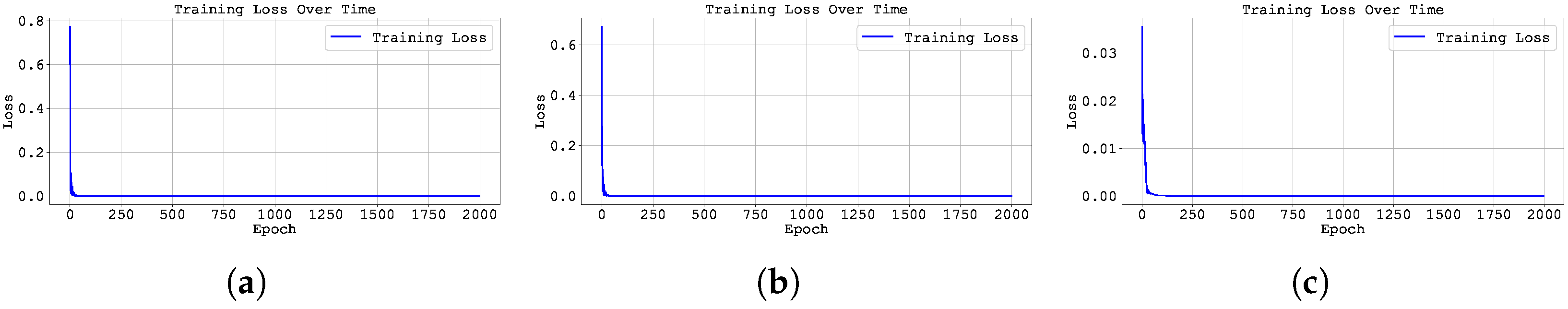
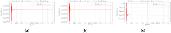
Figure A16.
Plot of the best run gradient value through training for Case Study 3, with , for (a) original, (b) clipped and (c) pre-trained Neural FDE.
Figure A16.
Plot of the best run gradient value through training for Case Study 3, with , for (a) original, (b) clipped and (c) pre-trained Neural FDE.
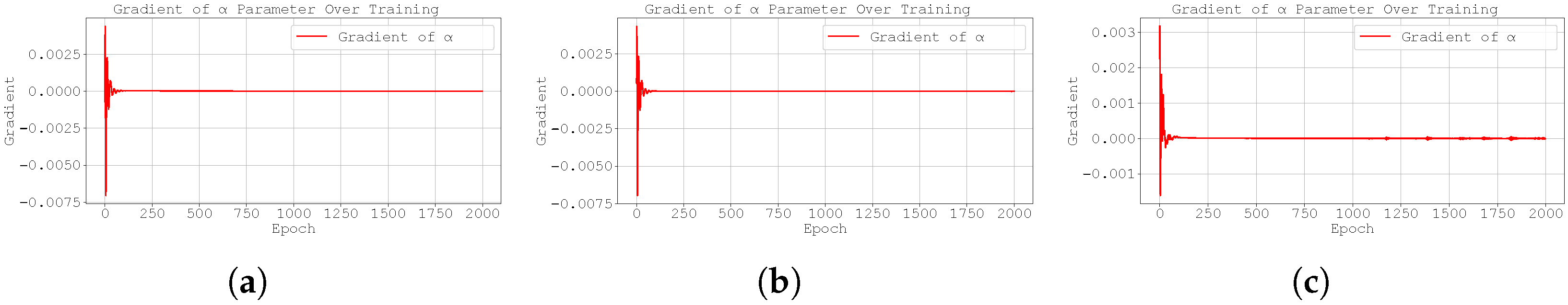
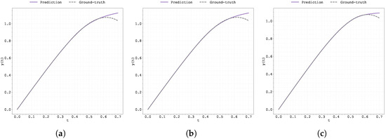
Figure A17.
Plot of the predicted and ground-truth curves from the best run in Case Study 3 with initialised at : (a) the original, (b) clipped, and (c) pre-trained Neural FDE models.
Figure A17.
Plot of the predicted and ground-truth curves from the best run in Case Study 3 with initialised at : (a) the original, (b) clipped, and (c) pre-trained Neural FDE models.
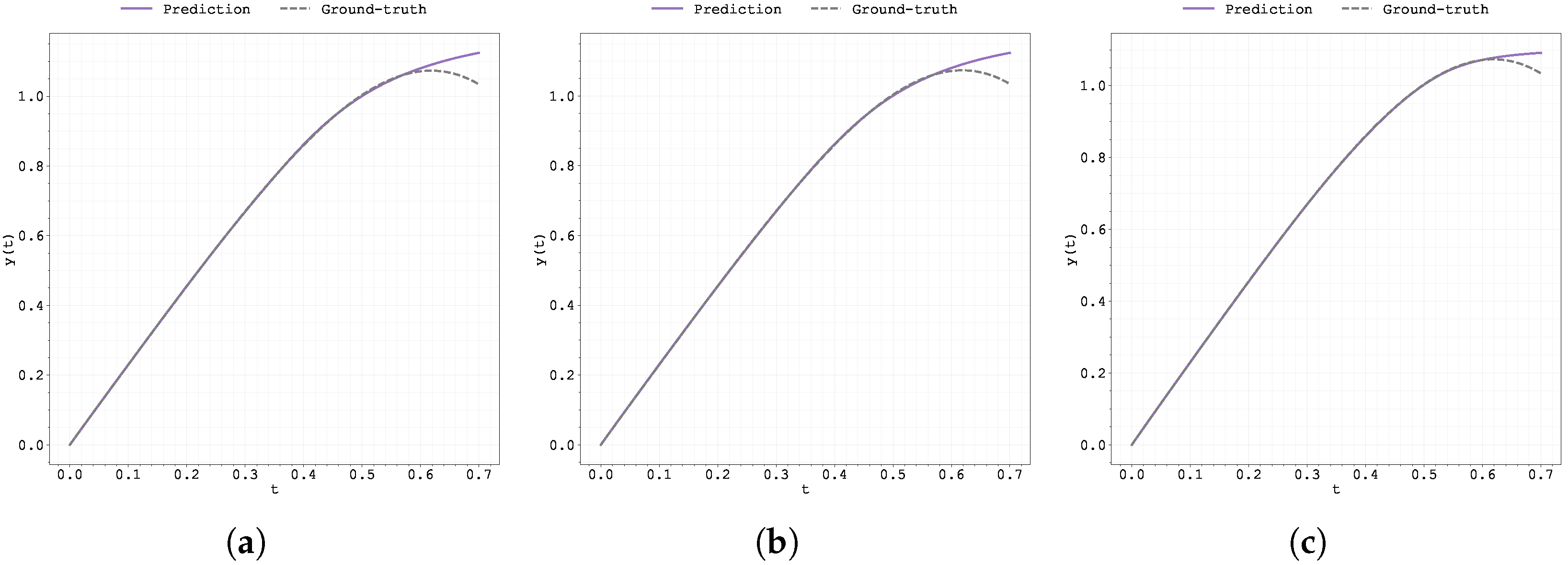
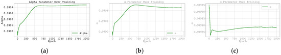
Figure A18.
Evolution of the best run’s during training for Case Study 3 with : (a) original Neural FDE, (b) clipped Neural FDE, and (c) pre-trained Neural FDE.
Figure A18.
Evolution of the best run’s during training for Case Study 3 with : (a) original Neural FDE, (b) clipped Neural FDE, and (c) pre-trained Neural FDE.
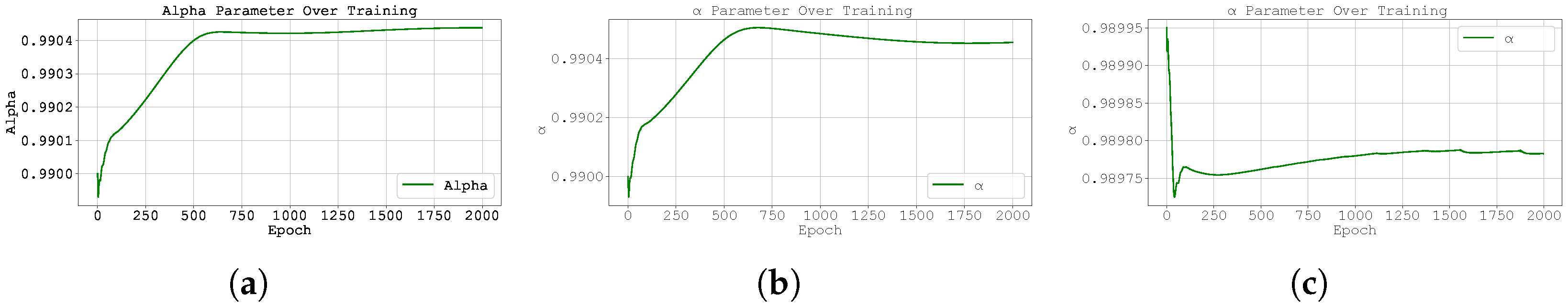
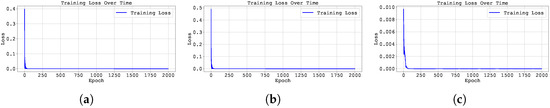
Figure A19.
Training loss across epochs for the best run in Case Study 2 with : (a) the original, (b) clipped, and (c) pre-trained Neural FDE models.
Figure A19.
Training loss across epochs for the best run in Case Study 2 with : (a) the original, (b) clipped, and (c) pre-trained Neural FDE models.
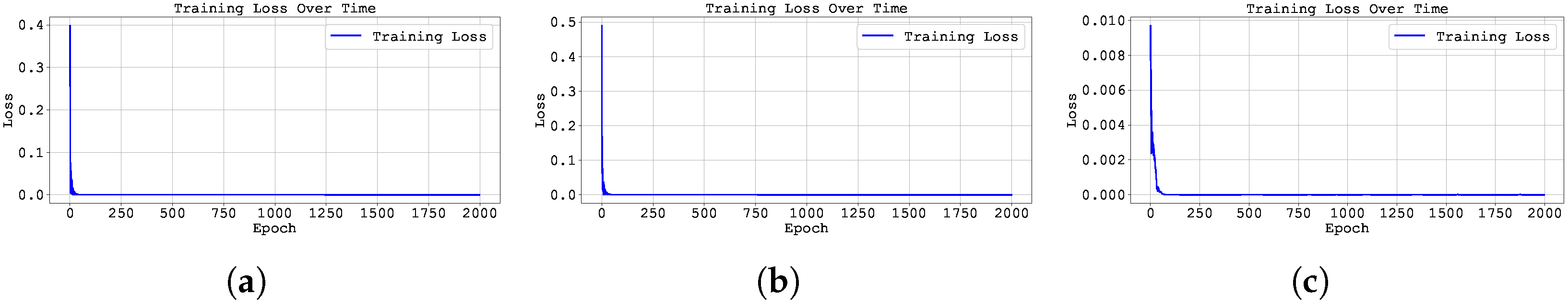
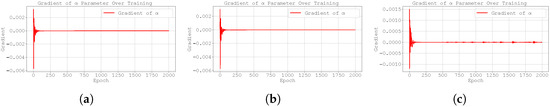
Figure A20.
Plot of the best run gradient value through training for Case Study 3, with , for (a) original, (b) clipped and (c) pre-trained Neural FDE.
Figure A20.
Plot of the best run gradient value through training for Case Study 3, with , for (a) original, (b) clipped and (c) pre-trained Neural FDE.
Appendix A.3. Case Study 4
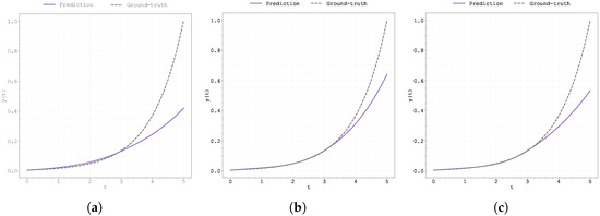
Figure A21.
Plot of the predicted and ground-truth curves from the best run in Case Study 4 with initialised at : (a) the original, (b) clipped, and (c) pre-trained Neural FDE models.
Figure A21.
Plot of the predicted and ground-truth curves from the best run in Case Study 4 with initialised at : (a) the original, (b) clipped, and (c) pre-trained Neural FDE models.
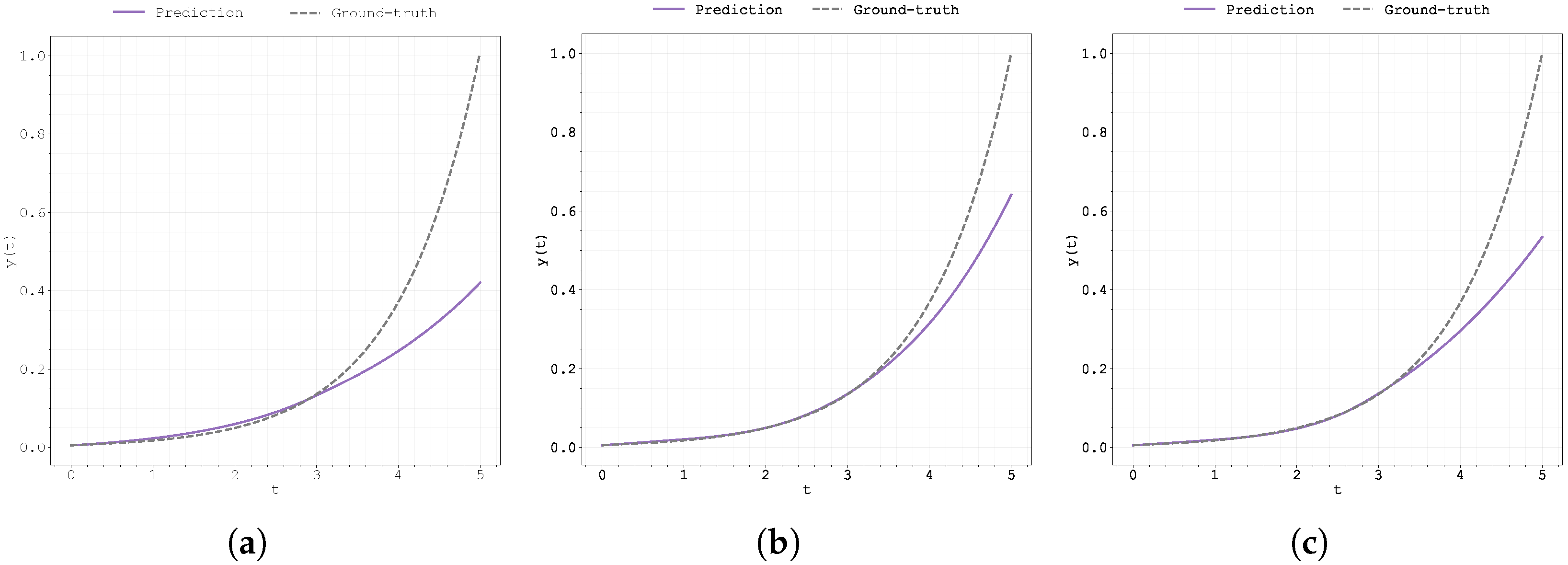
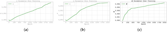
Figure A22.
Evolution of the best run’s during training for Case Study 4 with : (a) original Neural FDE, (b) clipped Neural FDE, and (c) pre-trained Neural FDE.
Figure A22.
Evolution of the best run’s during training for Case Study 4 with : (a) original Neural FDE, (b) clipped Neural FDE, and (c) pre-trained Neural FDE.
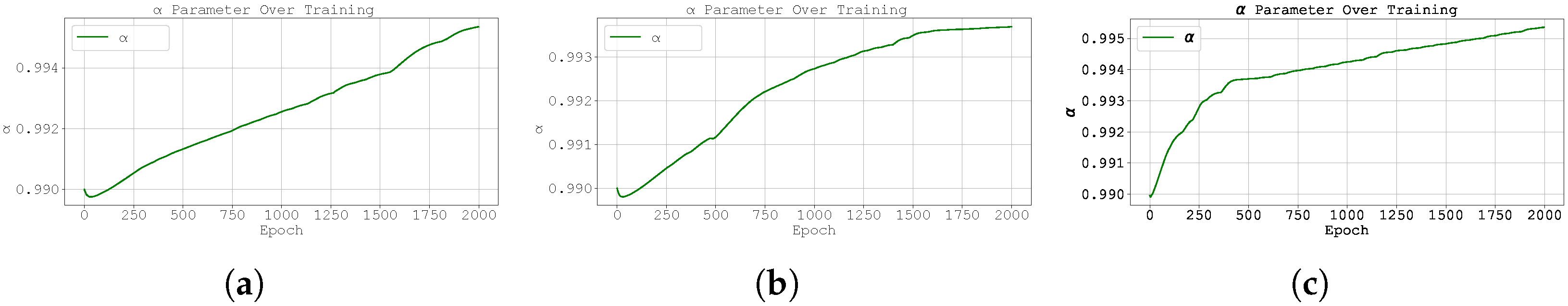
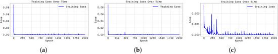
Figure A23.
Training loss across epochs for the best run in Case Study 4 with : (a) the original, (b) clipped, and (c) pre-trained Neural FDE models.
Figure A23.
Training loss across epochs for the best run in Case Study 4 with : (a) the original, (b) clipped, and (c) pre-trained Neural FDE models.
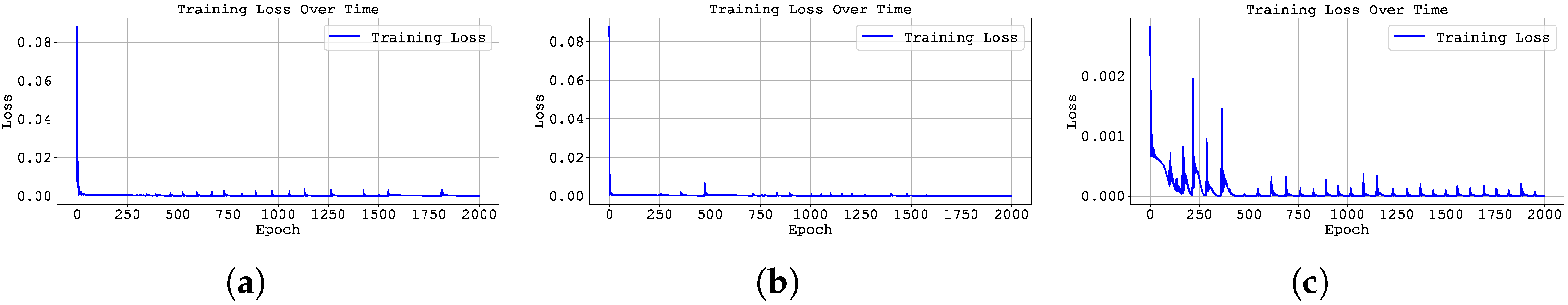
Figure A24.
Plot of the best run gradient value through training for Case Study 2, with , for (a) original, (b) clipped and (c) pre-trained Neural FDE.
Figure A24.
Plot of the best run gradient value through training for Case Study 2, with , for (a) original, (b) clipped and (c) pre-trained Neural FDE.
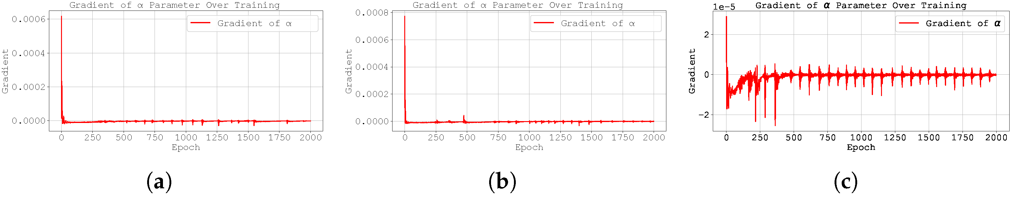
Figure A25.
Plot of the predicted and ground-truth curves from the best run in Case Study 4 with initialised at : (a) the original, (b) clipped, and (c) pre-trained Neural FDE models.
Figure A25.
Plot of the predicted and ground-truth curves from the best run in Case Study 4 with initialised at : (a) the original, (b) clipped, and (c) pre-trained Neural FDE models.
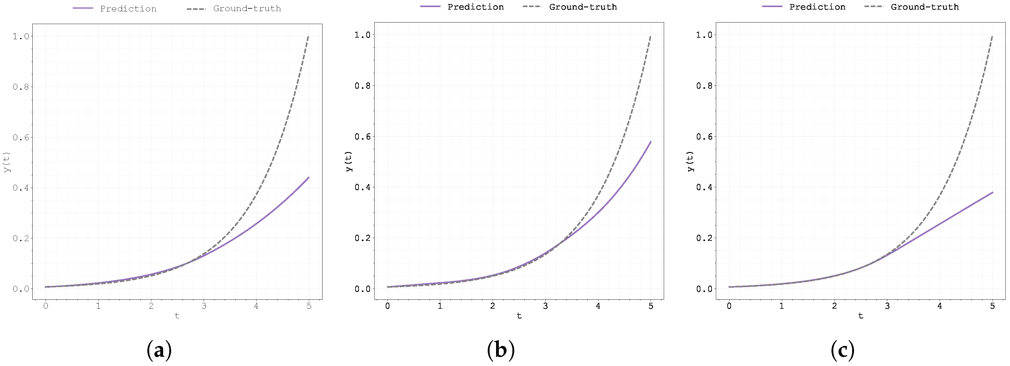
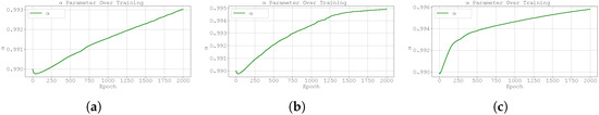
Figure A26.
Evolution of the best run’s during training for Case Study 4 with : (a) original Neural FDE, (b) clipped Neural FDE, and (c) pre-trained Neural FDE.
Figure A26.
Evolution of the best run’s during training for Case Study 4 with : (a) original Neural FDE, (b) clipped Neural FDE, and (c) pre-trained Neural FDE.
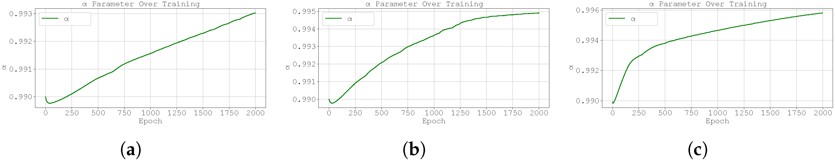
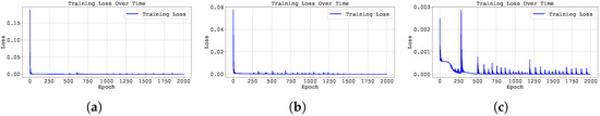
Figure A27.
Training loss across epochs for the best run in Case Study 4 with : (a) the original, (b) clipped, and (c) pre-trained Neural FDE models.
Figure A27.
Training loss across epochs for the best run in Case Study 4 with : (a) the original, (b) clipped, and (c) pre-trained Neural FDE models.
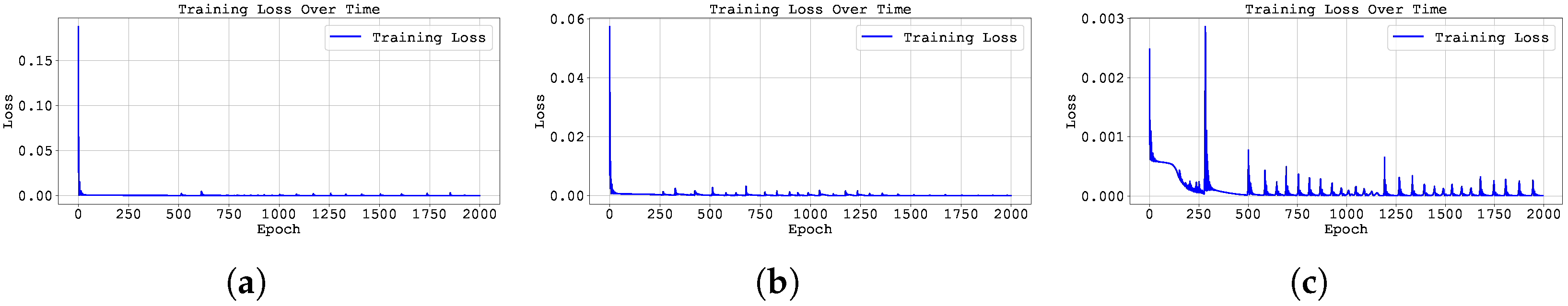
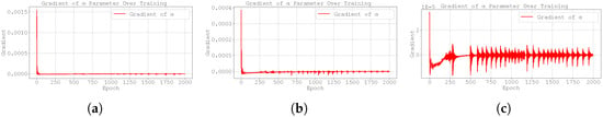
Figure A28.
Plot of the best run gradient value through training for Case Study 2, with , for (a) original, (b) clipped and (c) pre-trained Neural FDE.
Figure A28.
Plot of the best run gradient value through training for Case Study 2, with , for (a) original, (b) clipped and (c) pre-trained Neural FDE.
References
- Coelho, C.; Costa, M.F.P.; Ferrás, L.L. Tracing Footprints: Neural Networks Meet Non-integer Order Differential Equations For Modelling Systems with Memory. In Proceedings of the The Second Tiny Papers Track at ICLR 2024, Tiny Papers @ ICLR 2024, Vienna, Austria, 11 May 2024. [Google Scholar]
- Coelho, C.; Costa, M.F.P.; Ferrás, L.L. Neural Fractional Differential Equations. Appl. Math. Model. 2025, 144, 116060. [Google Scholar] [CrossRef]
- Kang, Q.; Zhao, K.; Ding, Q.; Ji, F.; Li, X.; Liang, W.; Song, Y.; Tay, W.P. Unleashing the potential of fractional calculus in graph neural networks with FROND. arXiv 2024, arXiv:2404.17099. [Google Scholar] [CrossRef]
- Cui, W.; Kang, Q.; Li, X.; Zhao, K.; Tay, W.P.; Deng, W.; Li, Y. Neural variable-order Fractional Differential Equation networks. In Proceedings of the AAAI Conference on Artificial Intelligence, Philadelphia, PA, USA, 25 February–4 March 4 2025; Volume 39, pp. 16109–16117. [Google Scholar]
- Vellappandi, M.; Lee, S. Physics-informed Neural Fractional Differential Equations. Appl. Math. Model. 2025, 145, 116127. [Google Scholar] [CrossRef]
- Kang, Q.; Li, X.; Zhao, K.; Cui, W.; Zhao, Y.; Deng, W.; Tay, W.P. Efficient training of neural fractional-order differential equation via adjoint backpropagation. In Proceedings of the AAAI Conference on Artificial Intelligence, Philadelphia, PA, USA, 25 February–4 March 2025; Volume 39, pp. 17750–17759. [Google Scholar]
- Zhang, X.; Zhang, L.; Wei, W.; Sun, Y.; Tian, C.; Zhang, Y. FDE-Net: A memory-efficiency densely connected network inspired from fractional-order differential equations for single image super-resolution. Neurocomputing 2024, 600, 128143. [Google Scholar] [CrossRef]
- Caputo, M. Linear Models of Dissipation whose Q is almost Frequency Independent—II. Geophys. J. Int. 1967, 13, 529–539. [Google Scholar] [CrossRef]
- Diethelm, K. The Analysis of Fractional Differential Equations: An Application-Oriented Exposition Using Differential Operators of Caputo Type; Springer: Berlin/Heidelberg, Germany, 2010. [Google Scholar] [CrossRef]
- Podlubny, I. Fractional Differential Equations: An Introduction to fRactional Derivatives, Fractional Differential Equations, to Methods of Their Solution and Some of Their Applications; Elsevier: Amsterdam, The Netherlands, 1998; Volume 198. [Google Scholar]
- Kilbas, A.A.; Srivastava, H.M.; Trujillo, J.J. Theory and Applications of Fractional Differential Equations; North-Holland Mathematics Studies; Elsevier Science & Technology: Amsterdam, The Netherlands, 2014. [Google Scholar]
- Jin, B. Fractional Differential Equations: An Approach via Fractional Derivatives; Springer International Publishing: Cham, Switzerland, 2021. [Google Scholar] [CrossRef]
- Zhou, Y.; Wang, J.; Zhang, L. Basic Theory of Fractional Differential Equations; WORLD SCIENTIFIC: Singapore, 2016. [Google Scholar] [CrossRef]
- Abbas, S.; Benchohra, M.; N’Guérékata, G.M. Topics in Fractional Differential Equations; Springer: New York, NY, USA, 2012. [Google Scholar] [CrossRef]
- Milici, C.; Drăgănescu, G.; Tenreiro Machado, J. Introduction to Fractional Differential Equations; Springer International Publishing: Cham, Switzerland, 2019. [Google Scholar] [CrossRef]
- Almeida, R.; Bastos, N.R.O.; Monteiro, M.T.T. Modeling some real phenomena by Fractional Differential Equations. Math. Methods Appl. Sci. 2015, 39, 4846–4855. [Google Scholar] [CrossRef]
- Chen, R.T.; Rubanova, Y.; Bettencourt, J.; Duvenaud, D.K. Neural ordinary differential equations. Adv. Neural Inf. Process. Syst. 2018, 31. [Google Scholar]
- Coelho, C.; Costa, M.F.P.; Ferrás, L.L. Neural Fractional Differential Equations: Optimising the Order of the Fractional Derivative. Fractal Fract. 2024, 8, 529. [Google Scholar] [CrossRef]
- Diethelm, K.; Ford, N.J. Analysis of Fractional Differential Equations. J. Math. Anal. Appl. 2002, 265, 229–248. [Google Scholar] [CrossRef]
- Zhang, J.; He, T.; Sra, S.; Jadbabaie, A. Why gradient clipping accelerates training: A theoretical justification for adaptivity. arXiv 2019, arXiv:1905.11881. [Google Scholar]
- Zhang, B.; Jin, J.; Fang, C.; Wang, L. Improved analysis of clipping algorithms for non-convex optimization. Adv. Neural Inf. Process. Syst. 2020, 33, 15511–15521. [Google Scholar]
- Jain, L.C.; Seera, M.; Lim, C.P.; Balasubramaniam, P. A review of online learning in supervised neural networks. Neural Comput. Appl. 2014, 25, 491–509. [Google Scholar] [CrossRef]
- Paszke, A.; Gross, S.; Massa, F.; Lerer, A.; Bradbury, J.; Chanan, G.; Killeen, T.; Lin, Z.; Gimelshein, N.; Antiga, L.; et al. PyTorch: An Imperative Style, High-Performance Deep Learning Library. In Advances in Neural Information Processing Systems 32; Wallach, H., Larochelle, H., Beygelzimer, A., d’Alché-Buc, F., Fox, E., Garnett, R., Eds.; Curran Associates, Inc.: Red Hook, NY, USA, 2019; pp. 8024–8035. [Google Scholar]
- Zimmering, B.; Coelho, C.; Niggemann, O. Optimising Neural Fractional Differential Equations for Performance and Efficiency. In Proceedings of the 1st ECAI Workshop on “Machine Learning Meets Differential Equations: From Theory to Applications”, Santiago de Compostela, Spain, 20 October 2024; Volume 255, pp. 1–22. [Google Scholar]
- Kingma, D.P.; Ba, J. Adam: A method for stochastic optimization. arXiv 2014, arXiv:1412.6980. [Google Scholar]
- Liu, Y.; Roberts, J.; Yan, Y. A note on finite difference methods for nonlinear fractional differential equations with non-uniform meshes. Int. J. Comput. Math. 2018, 95, 1151–1169. [Google Scholar] [CrossRef]
- Luo, C.; Wang, X. Chaos in the fractional-order complex Lorenz system and its synchronization. Nonlinear Dyn. 2012, 71, 241–257. [Google Scholar] [CrossRef]
- Yu, Y.; Li, H.X. The synchronization of fractional-order Rössler hyperchaotic systems. Phys. A Stat. Mech. Its Appl. 2008, 387, 1393–1403. [Google Scholar] [CrossRef]
- El-Wakil, S.A.; Abulwafa, E.M.; Zahran, M.A.; Mahmoud, A.A. Time-fractional KdV equation: Formulation and solution using variational methods. Nonlinear Dyn. 2011, 65, 55–63. [Google Scholar] [CrossRef]
- Laskin, N. Fractional schrödinger equation. Phys. Rev. E 2002, 66, 056108. [Google Scholar] [CrossRef] [PubMed]


Disclaimer/Publisher’s Note: The statements, opinions and data contained in all publications are solely those of the individual author(s) and contributor(s) and not of MDPI and/or the editor(s). MDPI and/or the editor(s) disclaim responsibility for any injury to people or property resulting from any ideas, methods, instructions or products referred to in the content. |
© 2025 by the authors. Licensee MDPI, Basel, Switzerland. This article is an open access article distributed under the terms and conditions of the Creative Commons Attribution (CC BY) license (https://creativecommons.org/licenses/by/4.0/).