Efficient Hybrid Parallel Scheme for Caputo Time-Fractional PDEs on Multicore Architectures

Abstract

We present a hybrid parallel scheme for efficiently solving Caputo time-fractional partial differential equations (CTFPDEs) with integer-order spatial derivatives on multicore CPU and GPU platforms. The approach combines a second-order spatial discretization with the $L1$ time-stepping scheme and employs MATLAB parfor parallelization to achieve significant reductions in runtime and memory usage. A theoretical third-order convergence rate is established under smooth-solution assumptions, and the analysis also accounts for the loss of accuracy near the initial time $t=t_0$ caused by weak singularities inherent in time-fractional models. Unlike many existing approaches that rely on locally convergent strategies, the proposed method ensures global convergence even for distant or randomly chosen initial guesses. Benchmark problems from fractional biological models—including glucose–insulin regulation, tumor growth under chemotherapy, and drug diffusion in tissue—are used to validate the robustness and reliability of the scheme. Numerical experiments confirm near-linear speedup on up to four CPU cores and show that the method outperforms conventional techniques in terms of convergence rate, residual error, iteration count, and efficiency. These results demonstrate the method’s suitability for large-scale CTFPDE simulations in scientific and engineering applications.

1. Introduction

The past few decades have witnessed rapid progress in computational biology, personalized medicine, and medical diagnostics, driven in part by advances in the modeling and simulation of biological processes [1,2,3]. Classical approaches, typically formulated through integer-order differential equations, have played a central role in describing many physiological phenomena. Yet, such models often fall short when applied to complex biological systems characterized by long-range spatial interactions, memory effects, anomalous transport, and nonlocal behavior—features that classical partial differential equations (PDEs) do not adequately capture. To overcome these limitations, Caputo time-fractional-order partial differential equations (CTFPDEs) have emerged as a flexible and powerful framework for the simulation of real-world problems in biomedical engineering [4,5].

CTFPDEs, defined by derivatives of non-integer order in time or space, provide an enriched modeling framework capable of capturing hereditary and memory-dependent properties inherent in many biological tissues and systems [6]. They naturally generalize classical integer-order models, allowing for a more faithful interpretation of experimental data in contexts such as anomalous drug diffusion [7], electrical signal propagation in cardiac tissue [8], viscoelastic behavior of soft biological materials [9], and neural signal transmission [10]. Despite these advantages, CTFPDEs also give rise to significant analytical and computational challenges, particularly in the presence of nonlinear dynamics, multi-scale geometries, or patient-specific parameters. A representative form of such equations is

$$\left\{\begin{array}{cc}{\displaystyle \frac{{\partial }^{\sigma }u}{\partial t^{\sigma }}}+{\displaystyle \frac{{\partial }^{2}u}{\partial x^2}}+{\displaystyle \frac{\partial u}{\partial x}}+u(x,t)=f(x,t),\hfill & x\in [x^{\left[0\right]},x^{\left[n\right]}],t\in [t^{\left[0\right]},t^{\left[n\right]}],\hfill \\ u(x,0)=g_1\left(x\right),\hfill \\ u(0,t)=g_2\left(t\right), u(L,t)=g_3\left(t\right).\hfill \end{array}\right.$$

(1)

where $\sigma \in (0,1]$ denotes the Caputo fractional order of the differential operator.

More generally, let

$$\Sigma =\sum _{i=1}^l{\sigma }_i, {\sigma }_i\in (m_i-1,m_i), m_i\in {\mathbb{Z}}^{+}, i=1,\dots ,l.$$

The Caputo fractional derivative of order $\Sigma$ with respect to the variables $(x_1,\dots ,x_l)$ is defined as [11]:

$${}_{ }{}^{C}D_{\gamma ,x_1^{{\sigma }_1},···,x_l^{{\sigma }_l}}^{\Sigma }f(t_1,\dots ,t_l)={\int }_{\gamma }^{x_l}\dots {\int }_{\gamma }^{x_1}{\displaystyle \frac{{\displaystyle \prod _{i=1}^l}{(t_i-{\xi }_i)}^{m_i-{\sigma }_i-1}{\displaystyle \frac{{\partial }^{m_1+···+m_l}f({\xi }_1,\dots ,{\xi }_l)}{\partial {\xi }_1^{m_1}···\partial {\xi }_l^{m_l}}}}{{\displaystyle \prod _{i=1}^l}\Gamma (m_i-{\sigma }_i)}}d{\xi }_1···d{\xi }_l,$$

(2)

where ${\sigma }_i$ denotes the fractional order associated with $x_i$, $m_i=\lceil {\sigma }_i\rceil$, and $\Gamma (·)$ is the Gamma function.

As a special case with $l=1$, we obtain the Caputo time-fractional derivative. For a function $u(x,t)$, the Caputo fractional derivative of order $\sigma$ with respect to time t is defined as

$${}_{ }{}^{C}D_t^{\sigma }u(x,t)={\displaystyle \frac{1}{\Gamma (m-\sigma )}}{\int }_0^t{(t-\tau )}^{m-\sigma -1}{\displaystyle \frac{{\partial }^{m}u}{\partial {\tau }^m}}(x,\tau )d\tau , m-1<\sigma <m,m=\lceil \sigma \rceil .$$

(3)

In particular, for $0<\sigma <1$, we recover the commonly used form

$${}_{ }{}^{C}D_t^{\sigma }u(x,t)={\displaystyle \frac{1}{\Gamma (1-\sigma )}}{\int }_0^t{(t-\tau )}^{-\sigma }{\displaystyle \frac{\partial u}{\partial \tau }}(x,\tau )d\tau .$$

(4)

Equations (1)–(4) illustrate the mathematical structure of CTFPDEs frequently encountered in biomedical modeling. Due to their complexity, such equations generally do not admit closed-form solutions. In addition, biological systems often give rise to highly nonlinear, stiff, and spatially inhomogeneous CTFPDEs [12]. The presence of memory terms further increases the computational cost, rendering traditional methods impractical for realistic simulations—particularly in high-dimensional or real-time settings. This work is motivated by the need to bridge this gap, addressing the lack of scalable, parallel, and memory-efficient numerical solvers for CTFPDEs in biomedical imaging [13,14].

A wide range of methods has been proposed to tackle these challenges, spanning exact and semi-analytical approaches to fully numerical techniques. Analytical methods such as Laplace and Fourier transforms [15], Mittag-Leffler representations [16], and Green’s functions [17] offer valuable theoretical insights, but their applicability is largely confined to a limited class of linear, time-invariant CTFPDEs with idealized boundary conditions. These approaches become inadequate when applied to realistic biomedical models that involve nonlinear reaction–diffusion systems, irregular domains, or patient-specific heterogeneities [18,19]. To address these limitations, various analytical approximation techniques have been proposed, including the Adomian decomposition method [20], homotopy perturbation method [21], variational iteration method [22], and the fractional reduced differential transform method [23]. These methods are commonly used for solving nonlinear CTFPDEs and can provide closed-form-like series solutions. However, they often suffer from convergence issues, slow series truncation, and limited applicability—typically being effective only for weakly nonlinear problems.

In biological systems, nonlinearity often arises from feedback loops, saturation effects, or bifurcation dynamics, rendering analytical methods either divergent or symbolically intractable. As a result, research efforts have increasingly focused on numerical approaches, including the finite difference method [24], finite element method [25], spectral methods [26], convolution quadrature [27], and fractional Runge–Kutta methods [28]. These techniques offer broader applicability and have been employed in modeling cardiac conduction, tumor growth, neural activity, and drug delivery.

Nevertheless, numerical schemes for CTFPDEs are substantially more challenging than those for integer-order equations. The nonlocal nature of fractional derivatives necessitates storing the entire solution history, leading to significant memory consumption and computational overhead, particularly in long-time or high-dimensional simulations. Additionally, such schemes are subject to stability constraints, discretization errors, and complications in the implementation of fractional boundary conditions—especially in complex biomedical geometries [29,30]. Despite sustained research efforts, many of these challenges remain unresolved.

The limited scalability, high memory requirements, and inadequate real-time performance of existing methods provide the primary motivation for developing novel high-performance computational techniques. To overcome these challenges, we adopt parallel computational methodologies specifically designed for CTFPDEs. In contrast to conventional schemes that rely on sequential time-stepping or global matrix assembly, parallel methods leverage modern hardware architectures—such as multi-core processors and GPUs—to evolve solution components concurrently in space and time. These approaches are particularly well suited to CTFPDEs, as they

• Alleviate memory bottlenecks by distributing historical data across processors;
• Accelerate convergence through the concurrent evaluation of memory integrals and local operators;
• Enable adaptive domain decomposition for efficient modeling of complex anatomical geometries;
• Support real-time simulations for applications such as drug-response prediction, ECG signal reconstruction, and patient-specific medical imaging.

This study introduces a new class of parallel iterative methods for nonlinear fractional partial differential equations (FPDEs), specifically designed to address the stiffness, degeneracy and memory-dependent dynamics commonly encountered in biomedical applications. The proposed methodology is based on the following key components:

• A generalized parallel fractional framework capable of handling Caputo-type time derivatives and nonlinear spatial operators;
• A domain-decomposed architecture that enables concurrent computation of local solution components, thereby reducing overall simulation time;
• A symbolic–numeric hybrid strategy, in which the nonlinear systems arising from CTFPDE discretizations are solved using Newton-type methods;
• Comprehensive evaluation metrics, including convergence rate, CPU usage, residual error dynamics, memory efficiency, and biological interpretability.

The efficiency and applicability of the proposed schemes are demonstrated through three biomedical case studies:

• A fractional cardiac conduction system with nonlinear reaction–diffusion terms;
• A dynamical model of depression incorporating feedback mechanisms and long-term memory;
• A sub-diffusion drug delivery model in layered biological tissues.

Overall, this study offers the following contributions in comparison to existing work:

• Problem Scope: We address CTFPDEs derived from biomedical models that exhibit spatial heterogeneity and memory effects, extending beyond the idealized benchmark problems commonly considered in the literature.
• Parallelization Strategy: The proposed schemes implement parfor-based parallelization in MATLAB, enabling efficient utilization of multi-core processors and yielding measurable reductions in computational time.
• Benchmarking and Validation: Comprehensive tests are conducted, encompassing comparisons with analytical solutions, performance benchmarks, and application-driven case studies, in order to confirm the accuracy and robustness of the proposed approach.

The remainder of this paper is organized as follows. Section 2 introduces the class of CTFPDEs under consideration and outlines the proposed parallel scheme, including its construction and preliminary analysis. Section 3 presents the theoretical foundations of the method, covering discretization procedures, memory management, and convergence results. It also details the computational implementation, including parallel matrix assembly, solver design, and performance evaluation. Benchmarking against standard methods is provided, along with three biomedical case studies that demonstrate the effectiveness of the proposed approach. For each case study, we discuss the biological background, the formulation of the fractional model, and the simulation results, including error analysis, stability assessment, and physiological validation. Finally, Section 4 concludes the paper by summarizing the main findings and highlighting the translational potential of the method for clinical applications.

2. Construction and Analysis of the Next-Generation Computational Schemes

Building on the contributions outlined above, we now turn to the construction and analysis of the proposed computational framework. The numerical solution of CTFPDEs provides a practical approach to modeling complex phenomena that are analytically intractable, particularly in biomedical applications. Such methods are essential for capturing memory effects, nonlocal interactions, and anomalous diffusion that characterize many physiological processes.

Spatial and temporal discretization can be performed using finite difference, finite element, spectral, or convolution quadrature methods, with suitable adaptations for handling nonlinearities, heterogeneous coefficients, and irregular boundary conditions. These procedures typically lead to a system of nonlinear equations of the form

$$\begin{array}{c}{f}_1\left(x_1,···,x_n\right)=0,\\ f_2\left(x_1,···,x_n\right)=0,\\ ⋮\\ f_n\left(x_1,···,x_n\right)=0,\end{array}$$

(5)

where each function $f_i$ maps a vector $\mathbf{x}={(x_1,x_2,\dots ,x_n)}^t\in {\mathbb{R}}^n$ to $\mathbb{R}$. Defining

$$\mathbf{F}\left(\mathbf{x}\right)={(f_1(\mathbf{x}),···,f_n(\mathbf{x}\left)\right)}^t$$

(6)

system (5) can be compactly written as $\mathbf{F}\left(\mathbf{x}\right)=0$.

Numerical techniques for solving CTFPDEs via the nonlinear system formulation in (6) are often classified as local methods, most notably the classical Newton method [31] and its higher-order extensions [32,33,34]. These methods offer high accuracy and fast local convergence in the neighborhood of a solution, but they are highly sensitive to the choice of initial guess and generally lack guarantees of global convergence. Representative higher-order schemes include:

(i) The two-step, third-order method of Noor et al. [35]:

$${\mathbf{x}}^{[\hslash +1]}={\mathbf{x}}^{[\hslash ]}-{\displaystyle \frac{\mathbf{F}({\mathbf{x}}^{[\hslash ]})}{{\mathbf{F}}^{\prime }\left({\mathbf{x}}^{[\hslash ]}\right)+3{\mathbf{F}}^{\prime }\left(\frac{{\mathbf{x}}^{[\hslash ]}+\mathbf{2}{\mathbf{y}}^{[\hslash ]}}{3}\right)}},$$

(7)

where

$${\mathbf{y}}^{[\hslash ]}={\mathbf{x}}^{[\hslash ]}-{\displaystyle \frac{\mathbf{F}\left({\mathbf{x}}^{[\hslash ]}\right)}{{\mathbf{F}}^{\prime }\left({\mathbf{x}}^{[\hslash ]}\right)}},$$

(8)

(ii) The third-order method of Dehgan [36]:

$${\mathbf{x}}^{[\hslash +1]}={\mathbf{x}}^{[\hslash ]}-{\displaystyle \frac{\frac{1}{2}\mathbf{F}\left(2{\mathbf{x}}^{[\hslash ]}-{\mathbf{y}}^{[\hslash ]}\right)-\frac{3}{2}\mathbf{F}\left({\mathbf{y}}^{[\hslash ]}\right)}{{\mathbf{F}}^{\prime }\left({\mathbf{y}}^{[\hslash ]}\right)}},$$

(9)

(iii) The super-cubic method of Darvishi et al. [37]:

$${\mathbf{x}}^{[\hslash +1]}={\mathbf{x}}^{[\hslash ]}-{\displaystyle \frac{\mathbf{F}\left({\mathbf{x}}^{[\hslash ]}\right)}{2}}\left({\displaystyle \frac{1}{{\mathbf{F}}^{\prime }\left({\mathbf{x}}^{[\hslash ]}\right)}}+{\displaystyle \frac{1}{{\mathbf{F}}^{\prime }\left({\mathbf{y}}^{[\hslash ]}\right)}}\right),$$

(10)

(iv) The third-order method of Sharma et al. [38]:

$${\mathbf{x}}^{[\hslash +1]}={\mathbf{x}}^{[\hslash ]}-\frac{1}{2}\left(-I+{\displaystyle \frac{9}{4}}{\displaystyle \frac{{\mathbf{F}}^{\prime }\left({\mathbf{x}}^{[\hslash ]}\right)}{{\mathbf{F}}^{\prime }\left({\mathbf{y}}^{[\hslash ]}\right)}}+{\displaystyle \frac{3}{4}}{\displaystyle \frac{{\mathbf{F}}^{\prime }\left({\mathbf{z}}^{[\hslash ]}\right)}{{\mathbf{F}}^{\prime }\left({\mathbf{x}}^{[\hslash ]}\right)}}\right){\displaystyle \frac{\mathbf{F}\left({\mathbf{x}}^{[\hslash ]}\right)}{{\mathbf{F}}^{\prime }\left({\mathbf{x}}^{[\hslash ]}\right)}},$$

(11)

where

$${\mathbf{z}}^{[\hslash ]}={\mathbf{x}}^{[\hslash ]}-{\displaystyle \frac{2}{3}}{\displaystyle \frac{\mathbf{F}\left({\mathbf{x}}^{[\hslash ]}\right)}{{\mathbf{F}}^{\prime }\left({\mathbf{x}}^{[\hslash ]}\right)}};$$

(v) The fourth-order method of Cordero et al. [39]:

$${\mathbf{x}}^{[\hslash +1]}={\mathbf{y}}^{[\hslash ]}-\left(2-{\displaystyle \frac{{\mathbf{F}}^{\prime }\left({\mathbf{y}}^{[\hslash ]}\right)}{{\mathbf{F}}^{\prime }\left({\mathbf{x}}^{[\hslash ]}\right)}}\right){\displaystyle \frac{\mathbf{F}\left({\mathbf{x}}^{[\hslash ]}\right)}{{\mathbf{F}}^{\prime }\left({\mathbf{x}}^{[\hslash ]}\right)}}.$$

(12)

Several other single- and multi-step iterative methods for solving (6) have been proposed; see, for example, refs. [40,41,42,43] and the references therein. These conventional solvers, however, remain highly sensitive to the choice of initial guess and may fail to converge for strongly nonlinear or ill-conditioned systems. Their convergence is typically local and can be affected by parameter perturbations. For large-scale problems, repeated evaluations of the function and Jacobian lead to substantial computational overhead. Furthermore, their inherently sequential structure limits scalability, reducing their effectiveness for high-dimensional or time-dependent problems encountered in practice.

To address these limitations, we turn to parallel techniques that distribute computational tasks across multiple processors to achieve faster runtimes. Such approaches also enhance resilience and scalability, making them well suited for solving large nonlinear systems. One example is a generalized version of the classical Weierstrass–Durand–Kerner (WDK) method [44], which can be written as

$$\begin{gathered} {\mathbf{x}}_i^{[\hslash +1]}={\mathbf{x}}_i^{[\hslash ]}-{\displaystyle \frac{\mathbf{F}\left({\mathbf{x}}_j^{[\hslash ]}\right)}{{\prod }_{\begin{array}{c}t=1 \\ t\ne i\end{array}}^n\mathbf{G}({\mathbf{x}}_i^{[\hslash ]},{\mathbf{x}}_t^{[\hslash ]})}}, \end{gathered}$$

(13)

and which converges quadratically to the exact solution of (6). Here, $\mathbf{G}({\mathbf{x}}_i^{[\hslash ]},{\mathbf{x}}_t^{[\hslash ]})$ computes the WDK updates to find all solutions simultaneously, with $\mathbf{x}\in {\mathbb{C}}^n$ and $\mathbf{F}:{\mathbb{C}}^n\to {\mathbb{C}}^n$ We refer to method (13) as WDM^[C₂].

A generalized version of the Abreth–Ehrlich method [45] for solving (6), denoted ELM^[C₃], is given by

$${\mathbf{x}}_i^{[\hslash +1]}={\mathbf{x}}_i^{[\hslash ]}-{\displaystyle \frac{\mathbf{F}\left({\mathbf{x}}_i^{[\hslash ]}\right)}{\left(\frac{J_{\mathbf{F}}\left({\alpha }_i\right)}{\mathbf{F}\left({\mathbf{x}}_i^{[\hslash ]}\right)}-{\sum }_{\begin{array}{c}t=1\\ t\ne i\end{array}}^{d_i}\left(\frac{1}{{\mathbf{x}}_i^{[\hslash ]}-{\mathbf{x}}_t^{[\hslash ]}}\right)\right)\mathbf{F}\left({\mathbf{x}}_i^{[\hslash ]}\right)}},$$

(14)

where

$${\displaystyle \frac{J_{\mathbf{F}}\left({\alpha }_i\right)}{\mathbf{F}\left({\mathbf{x}}_i^{[\hslash ]}\right)}}={\displaystyle \frac{J_{\mathbf{F}}\left({\alpha }_i\right){\mathbf{F}}^T\left({\mathbf{x}}_i^{[\hslash ]}\right)}{{\mathbf{F}}^T\left({\mathbf{x}}_i^{[\hslash ]}\right)\mathbf{F}\left({\mathbf{x}}_i^{[\hslash ]}\right)}},$$

and

$$J_{\mathbf{F}}\left({\alpha }_i\right)=\left[\begin{array}{cccc}{\displaystyle \frac{\partial f_1}{\partial x_1}}& {\displaystyle \frac{\partial f_1}{\partial x_2}}& \dots & {\displaystyle \frac{\partial f_1}{\partial x_n}}\\ {\displaystyle \frac{\partial f_2}{\partial x_1}}& {\displaystyle \frac{\partial f_2}{\partial x_2}}& \dots & {\displaystyle \frac{\partial f_2}{\partial x_n}}\\ ⋮& ⋮& \ddots & ⋮\\ {\displaystyle \frac{\partial f_n}{\partial x_1}}& {\displaystyle \frac{\partial f_n}{\partial x_2}}& \dots & {\displaystyle \frac{\partial f_n}{\partial x_n}}\end{array}\right].$$

Cordero et al. [46] proposed a parallel scheme with convergence order $2p$ (for $p=1$), expressed as

$$\begin{gathered} {\displaystyle {\mathbf{x}}_i^{[\hslash +1]}={\mathbf{x}}_i^{[\hslash ]}-\frac{\mathbf{F}\left({\mathbf{x}}_i^{[\hslash ]}\right)}{{\displaystyle \mathbf{F}\left[{\mathbf{x}}_i^{[\hslash ]},{\mathbf{x}}_i^{[\hslash ]}+\beta \mathbf{F}\left({\mathbf{x}}_i^{[\hslash ]}\right)\right]-\mathbf{F}\left({\mathbf{x}}_i^{[\hslash ]}\right){\displaystyle \sum _{\begin{array}{c}t=1 \\ t\ne i\end{array}}^{d_i}}\left(\frac{1}{{\mathbf{x}}_i^{[\hslash ]}-{\mathbf{x}}_t^{[\hslash ]}}\right)}},} \end{gathered}$$

(15)

where ${\mathbf{x}}_i^{[\hslash ]}\in \mathbb{R}$ We refer to method (15) as ACM^[C₂].

Building on these earlier methods, the present work seeks to improve efficiency, stability, and scalability in solving nonlinear systems arising from CTFPDEs. The proposed scheme is examined through memory complexity estimates, stability analysis, and convergence theorems, thereby ensuring both theoretical rigor and practical feasibility.

2.1. Construction of the Scheme

Motivated by the methods discussed above, the primary goal of this study is to develop more efficient variants of single-step and two-step parallel techniques. The proposed single-step scheme is defined as

$${\mathbf{x}}_i^{\left[\hslash +1\right]}={\mathbf{x}}_i^{\left[\hslash \right]}-{\displaystyle \frac{\mathbf{F}\left({\mathbf{x}}_j^{\left[\hslash \right]}\right)}{\underset{\stackrel{t=1}{t\ne i}}{\stackrel{n}{\Pi }}\mathbf{G}({\mathbf{x}}_i^{\left[\hslash \right]},{\mathbf{z}}_t^{\left[\hslash \right]})}},$$

(16)

where

$${\mathbf{z}}_t^{\left[\hslash \right]}={\mathbf{x}}_t^{\left[\hslash \right]}-{\displaystyle \frac{\mathbf{F}\left({\mathbf{x}}_j^{\left[\hslash \right]}\right)}{{\mathbf{F}}^{\prime }\left({\mathbf{x}}_j^{\left[\hslash \right]}\right)}}.$$

We refer to method (16) as ${\mathrm{CMM}}_1^{\left[C_3\right]}$.

Building on this formulation, we construct a two-step parallel method given by

$${\mathbf{x}}_i^{[\hslash +1]}={\mathbf{y}}_i^{[\hslash ]}-\left(2I-{\displaystyle \frac{\underset{\stackrel{t=1}{t\ne i}}{\stackrel{n}{\Pi }}\mathbf{G}({\mathbf{y}}_i^{\left[\hslash \right]},{\mathbf{y}}_t^{\left[\hslash \right]})}{\underset{\stackrel{t=1}{t\ne i}}{\stackrel{n}{\Pi }}\mathbf{G}({\mathbf{x}}_i^{\left[\hslash \right]},{\mathbf{z}}_t^{\left[\hslash \right]})}}\right){\displaystyle \frac{\mathbf{F}\left({\mathbf{x}}_i^{[\hslash ]}\right)}{\underset{\stackrel{t=1}{t\ne i}}{\stackrel{n}{\Pi }}\mathbf{G}({\mathbf{x}}_i^{\left[\hslash \right]},{\mathbf{z}}_t^{\left[\hslash \right]})}},$$

(17)

where

$${\mathbf{y}}_i^{\left[\hslash \right]}={\mathbf{x}}_i^{\left[\hslash \right]}-{\displaystyle \frac{\mathbf{F}\left({\mathbf{x}}_j^{\left[\hslash \right]}\right)}{\underset{\stackrel{t=1}{t\ne i}}{\stackrel{n}{\Pi }}\mathbf{G}({\mathbf{x}}_i^{\left[\hslash \right]},{\mathbf{z}}_t^{\left[\hslash \right]})}}.$$

We refer to method (17) as ${\mathrm{CMM}}_2^{\left[C_3\right]}$.

2.2. Theoretical Convergence Analysis

The convergence of parallel iterative algorithms is typically established through local convergence analysis, which guarantees convergence to the exact solution of (6) provided that the initial guess is sufficiently close. Such analysis not only determines the order of convergence but also offers valuable guidance for designing stable and efficient algorithms. In high-performance computing contexts, local convergence analysis plays a key role in preventing divergence, enhancing robustness, and ensuring consistent performance across processors, particularly when synchronization is required for large-scale nonlinear problems.

Theorem 1. 

Let$\mathit{\alpha }=({\alpha }_1,\dots ,{\alpha }_n)$denote the solutions of nonlinear system (5). If the initial approximations${\mathbf{x}}_1^{\left[0\right]},\dots ,{\mathbf{x}}_n^{\left[0\right]}$are sufficiently close to and distinct from the exact solutions, then method ${\mathit{WDM}}^{\left[C_2\right]}$ converges with order 2.

Proof. 

Define the errors

$${\mathbf{e}}_i^{[\hslash ]}={\mathbf{x}}_i^{[\hslash ]}-{\alpha }_i,{\mathbf{e}}_i^{[\hslash +1]}={\mathbf{x}}_i^{[\hslash +1]}-{\alpha }_i.$$

Then,

$$\begin{gathered} {\mathbf{x}}_i^{[\hslash +1]}-{\alpha }_i={\mathbf{x}}_i^{[\hslash ]}-{\alpha }_i-{\displaystyle \frac{\mathbf{F}\left(x_i^{[\hslash ]}\right)}{{\prod }_{\begin{array}{c}t=1 \\ t\ne i\end{array}}^n\mathbf{G}({\mathbf{x}}_i^{[\hslash ]},{\mathbf{x}}_t^{[\hslash ]})}}, \end{gathered}$$

(18)

which implies

$$\begin{gathered} {\mathbf{e}}_i^{[\hslash +1]}={\mathbf{e}}_i^{[\hslash ]}-{\displaystyle \frac{\mathbf{F}\left(x_i^{[\hslash ]}\right)}{{\prod }_{\begin{array}{c}t=1 \\ t\ne i\end{array}}^n\mathbf{G}({\mathbf{x}}_i^{[\hslash ]},{\mathbf{x}}_t^{[\hslash ]})}}. \end{gathered}$$

(19)

A Taylor expansion gives

$$\mathbf{F}\left({\mathbf{x}}_j^{[\hslash ]}\right)=J_{\mathbf{F}}\left({\alpha }_i\right){\mathbf{e}}_i^{[\hslash ]}+O\left(\parallel {\mathbf{e}}_i^{[\hslash ]}{\parallel }^2\right),$$

(20)

where $J_{\mathbf{F}}\left({\alpha }_i\right)$ denotes the Jacobian of $\mathbf{F}$ at ${\alpha }_i$, assumed to be nonsingular. Similarly,

$$\begin{gathered} {\displaystyle \prod _{\begin{array}{c}t=1 \\ t\ne i\end{array}}^n}\mathbf{G}({\mathbf{x}}_i^{[\hslash ]},{\mathbf{x}}_t^{[\hslash ]})={\mathbf{D}}_i+O\left(\underset{i}{max}{\parallel {\mathbf{e}}_i^{[\hslash ]}\parallel }^2\right), \end{gathered}$$

(21)

with ${\mathbf{D}}_i\ne 0$. Substituting into (19) yields

$${\mathbf{e}}_i^{[\hslash +1]}={\mathbf{e}}_i^{[\hslash ]}-{\displaystyle \frac{J_{\mathbf{F}}\left({\alpha }_i\right){\mathbf{e}}_i^{[\hslash ]}+O(\parallel {\mathbf{e}}_i^{[\hslash ]}{\parallel }^2)}{{\mathbf{D}}_i+ O({max}_t\parallel {\mathbf{e}}_t^{[\hslash ]}\parallel )}}+\mathrm{higher-order}\mathrm{terms}.$$

(22)

Assuming $\parallel {\mathbf{e}}_i^{[\hslash ]}\parallel \approx \parallel {\mathbf{e}}_t^{[\hslash ]}\parallel$, we obtain

$$\begin{array}{cc}\hfill {\mathbf{e}}_i^{[\hslash +1]}& ={\mathbf{e}}_i^{[\hslash ]}O\left(\underset{t}{max}\parallel {\mathbf{e}}_t^{[\hslash ]}\parallel \right),\hfill \end{array}$$

(23)

$$\begin{array}{cc}\hfill & =O\left(\underset{t}{max}{\parallel {\mathbf{e}}_t^{[\hslash ]}\parallel }^2\right).\hfill \end{array}$$

(24)

Hence, the method converges quadratically.    □

Theorem 2. 

Let ${\alpha }_1,\dots ,{\alpha }_n$ denote the solutions of nonlinear system (5). If the initial approximations ${\mathbf{x}}_1^{\left[0\right]},\dots ,{\mathbf{x}}_n^{\left[0\right]}$ are sufficiently close to and distinct from the exact solutions, then method ${\mathit{CMM}}_1^{\left[C_3\right]}$ converges with order 3.

Proof. 

Define the errors

$${\mathbf{e}}_i^{[\hslash ]}={\mathbf{x}}_i^{[\hslash ]}-{\alpha }_i,{\mathbf{e}}_i^{[\hslash +1]}={\mathbf{x}}_i^{[\hslash +1]}-{\alpha }_i.$$

Then,

$$\begin{gathered} {\mathbf{x}}_i^{[\hslash +1]}-{\alpha }_i={\mathbf{x}}_i^{[\hslash ]}-{\alpha }_i-{\displaystyle \frac{\mathbf{F}\left(x_i^{[\hslash ]}\right)}{{\prod }_{\begin{array}{c}t=1 \\ t\ne i\end{array}}^n\mathbf{G}({\mathbf{x}}_i^{[\hslash ]},{\mathbf{z}}_t^{[\hslash ]})}}, \end{gathered}$$

(25)

which implies

$$\begin{gathered} {\mathbf{e}}_i^{[\hslash +1]}={\mathbf{e}}_i^{[\hslash ]}-{\displaystyle \frac{\mathbf{F}\left(x_i^{[\hslash ]}\right)}{{\prod }_{\begin{array}{c}t=1 \\ t\ne i\end{array}}^n\mathbf{G}({\mathbf{x}}_i^{[\hslash ]},{\mathbf{z}}_t^{[\hslash ]})}}. \end{gathered}$$

A Taylor expansion yields

$$\mathbf{F}({\mathbf{x}}_j^{[\hslash ]})=J_{\mathbf{F}}({\alpha }_i){\mathbf{e}}_i^{[\hslash ]}+{\mathbf{R}}_i({\mathbf{e}}_i^{[\hslash ]}),$$

(26)

where

• $J_{\mathbf{F}}\left({\alpha }_i\right)$ is the Jacobian of $\mathbf{F}$ at ${\alpha }_i$, assumed nonsingular;
• ${\mathbf{R}}_i({\mathbf{e}}_i^{[\hslash ]})$ collects higher-order terms, with ${\mathbf{R}}_i({\mathbf{e}}_i^{[\hslash ]})=O(\parallel {\mathbf{e}}_i^{[\hslash ]}{\parallel }^2)$.

Expanding ${\prod }_{\begin{array}{c}t=1\\ t\ne i\end{array}}^n\mathbf{G}({\mathbf{x}}_i^{[\hslash ]},{\mathbf{z}}_t^{[\hslash ]})$ around the solution and assuming it is nonzero and continuous near ${\zeta }_i$, we obtain

$$\begin{gathered} {\displaystyle \prod _{\begin{array}{c}t=1 \\ t\ne i\end{array}}^n}\mathbf{G}({\mathbf{x}}_i^{[\hslash ]},{\mathbf{z}}_t^{[\hslash ]})={\mathbf{D}}_i^{[\hslash ]}+{\mathbf{S}}_j\left({\mathbf{e}}_i^{[\hslash ]}\right), \end{gathered}$$

(27)

where ${\mathbf{D}}_i^{[\hslash ]}\ne 0$, and 

$${\mathbf{S}}_j({\mathbf{e}}_i^{[\hslash ]})=O\left(\underset{t}{max}{\parallel {\mathbf{e}}_t^{[\hslash ]}\parallel }^2\right).$$

(28)

Hence,

$$\begin{gathered} {\displaystyle \prod _{\begin{array}{c}t=1 \\ t\ne i\end{array}}^n}\mathbf{G}({\mathbf{x}}_i^{[\hslash ]},{\mathbf{z}}_t^{[\hslash ]})={\mathbf{D}}_i+O\left(\underset{t}{max}{\parallel {\mathbf{e}}_t^{[\hslash ]}\parallel }^2\right). \end{gathered}$$

(29)

Since $J_{\mathbf{F}}\left({\alpha }_i\right)$ is invertible and bounded, and $1/{\mathbf{D}}_i$ is also bounded, it follows that

$$\begin{gathered} {\mathbf{e}}_i^{[\hslash +1]}={\mathbf{e}}_i^{[\hslash ]}-{\displaystyle \frac{J_{\mathbf{F}}\left({\alpha }_i\right){\mathbf{e}}_i^{[\hslash ]}+{\mathbf{R}}_i\left({\mathbf{e}}_i^{[\hslash ]}\right)}{{\prod }_{\begin{array}{c}t=1 \\ t\ne i\end{array}}^n\mathbf{G}({\mathbf{x}}_i^{[\hslash ]},{\mathbf{z}}_t^{[\hslash ]})}}+\mathrm{higher-order}\mathrm{terms}, \end{gathered}$$

(30)

or equivalently,

$${\mathbf{e}}_i^{[\hslash +1]}={\mathbf{e}}_i^{[\hslash ]}-{\displaystyle \frac{J_{\mathbf{F}}\left({\alpha }_i\right){\mathbf{e}}_i^{[\hslash ]}+{\mathbf{R}}_i\left({\mathbf{e}}_i^{[\hslash ]}\right)}{{\mathbf{D}}_i^{[\hslash ]}+{\mathbf{S}}_t\left({\mathbf{e}}_t^{[\hslash ]}\right)}}+\mathrm{higher-order}\mathrm{terms}.$$

(31)

Assuming $\parallel {\mathbf{e}}_i^{[\hslash ]}\parallel =\parallel {\mathbf{e}}_t^{[\hslash ]}\parallel =\parallel {\mathbf{e}}^{[\hslash ]}\parallel$, we obtain

$$\begin{array}{cc}\hfill {\mathbf{e}}_i^{[\hslash +1]}& ={\mathbf{e}}_i^{[\hslash ]}O\left(\underset{t}{max}{\parallel {\mathbf{e}}_t^{[\hslash ]}\parallel }^2\right),\hfill \end{array}$$

(32)

$$\begin{array}{cc}\hfill & =O\left(\parallel {\mathbf{e}}^{[\hslash ]}{\parallel }^3\right).\hfill \end{array}$$

(33)

Therefore, method ${\mathrm{CMM}}_1^{\left[C_3\right]}$ converges cubically.    □

Theorem 3. 

Let ${\mathit{\alpha }}_1,\dots ,{\mathit{\alpha }}_{\sigma }$ be simple solutions of (5). If the initial approximations ${\mathbf{x}}_1^{\left[0\right]},\dots ,{\mathbf{x}}_n^{\left[0\right]}$ are sufficiently close to and distinct from these roots, then method ${\mathit{CMM}}_2^{\left[C_3\right]}$ converges with order 3.

Proof. 

Define the errors

$${\mathbf{e}}_{ix}^{[\hslash ]}={\mathbf{x}}_i^{[\hslash ]}-{\mathit{\alpha }}_i,{\mathbf{e}}_{iy}^{[\hslash ]}={\mathbf{y}}_i^{[\hslash ]}-{\mathit{\alpha }}_i,{\mathbf{e}}_i^{[\hslash +1]}={\mathbf{x}}_i^{[\hslash +1]}-{\mathit{\alpha }}_i.$$

Then,

$${\mathbf{y}}_i^{\left[j\right]}-{\mathit{\alpha }}_i={\mathbf{x}}_i^{\left[j\right]}-{\mathit{\alpha }}_i-{\displaystyle \frac{\mathbf{F}\left({\mathbf{x}}_i^{\left[j\right]}\right)}{\underset{\stackrel{t=1}{t\ne i}}{\stackrel{n}{\Pi }}\mathbf{G}({\mathbf{x}}_i^{\left[j\right]},{\mathbf{z}}_t^{\left[j\right]})}},$$

(34)

and a Taylor expansion gives

$$\mathbf{F}\left({\mathbf{x}}_j^{[\hslash ]}\right)=J_{\mathbf{F}}\left({\mathit{\alpha }}_i\right){\mathbf{e}}_i^{[\hslash ]}+{\mathbf{R}}_i\left({\mathbf{e}}_i^{[\hslash ]}\right),$$

(35)

where

• $J_{\mathbf{F}}\left({\mathit{\alpha }}_i\right)$ is the Jacobian of $\mathbf{F}$ evaluated at ${\mathit{\alpha }}_i$, assumed nonsingular;
• ${\mathbf{R}}_i\left({\mathbf{e}}_i^{[\hslash ]}\right)$ collects the higher-order terms, with ${\mathbf{R}}_i\left({\mathbf{e}}_i^{[\hslash ]}\right)=O(\parallel {\mathbf{e}}_i^{[\hslash ]}{\parallel }^2)$.

Expanding ${\prod }_{\begin{array}{c}t=1\\ t\ne i\end{array}}^n\mathbf{G}({\mathbf{x}}_i^{[\hslash ]},{\mathbf{z}}_t^{[\hslash ]})$ around the solution and assuming it is nonzero and continuous near ${\zeta }_i$, we obtain

$$\begin{gathered} {\displaystyle \prod _{\begin{array}{c}t=1 \\ t\ne i\end{array}}^n}\mathbf{G}({\mathbf{x}}_i^{[\hslash ]},{\mathbf{z}}_t^{[\hslash ]})={\mathbf{D}}_i^{[\hslash ]}+{\mathbf{S}}_t\left({\mathbf{e}}_t^{[\hslash ]}\right), \end{gathered}$$

(36)

where ${\mathbf{D}}_i^{[\hslash ]}\ne 0$, and 

$${\mathbf{S}}_j\left({\mathbf{e}}_{ix}^{[\hslash ]}\right)=O\left(\underset{t}{max}{\parallel {\mathbf{e}}_{tx}^{[\hslash ]}\parallel }^2\right).$$

(37)

Hence,

$$\begin{gathered} {\displaystyle \prod _{\begin{array}{c}t=1 \\ t\ne i\end{array}}^n}\mathbf{G}({\mathbf{x}}_i^{[\hslash ]},{\mathbf{z}}_t^{[\hslash ]})={\mathbf{D}}_i+O\left(\underset{t}{max}{\parallel {\mathbf{e}}_{tx}^{[\hslash ]}\parallel }^2\right). \end{gathered}$$

(38)

Since $J_{\mathbf{F}}\left({\mathit{\alpha }}_i\right)$ is invertible and bounded, and $1/{\mathbf{D}}_i$ is also bounded, it follows that

$$\begin{gathered} {\mathbf{e}}_{iy}^{[\hslash ]}={\mathbf{e}}_{ix}^{[\hslash ]}-{\displaystyle \frac{J_{\mathbf{F}}\left({\mathit{\alpha }}_i\right){\mathbf{e}}_i^{[\hslash ]}+{\mathbf{R}}_i\left({\mathbf{e}}_i^{[\hslash ]}\right)}{{\prod }_{\begin{array}{c}t=1 \\ t\ne i\end{array}}^n\mathbf{G}({\mathbf{x}}_i^{[\hslash ]},{\mathbf{z}}_t^{[\hslash ]})}}+\mathrm{higher-order}\mathrm{terms}. \end{gathered}$$

(39)

$${\mathbf{e}}_{iy}^{[\hslash +1]}={\mathbf{e}}_{ix}^{[\hslash ]}-{\displaystyle \frac{J_{\mathbf{F}}\left({\mathit{\alpha }}_i\right){\mathbf{e}}_{ix}^{[\hslash ]}+{\mathbf{R}}_i\left({\mathbf{e}}_{ix}^{[\hslash ]}\right)}{{\mathbf{D}}_i^{[\hslash ]}+{\mathbf{S}}_t\left({\mathbf{e}}_{tx}^{[\hslash ]}\right)}}+\mathrm{higher-order}\mathrm{terms}.$$

(40)

Thus,

$${\mathbf{e}}_i^{[\hslash +1]}={\mathbf{e}}_i^{[\hslash ]}O\left(\underset{t}{max}{\parallel {\mathbf{e}}_t^{[\hslash ]}\parallel }^2\right).$$

(41)

Assuming $\parallel {\mathbf{e}}_{ix}^{[\hslash ]}\parallel =\parallel {\mathbf{e}}_{tx}^{[\hslash ]}\parallel =\parallel {\mathbf{e}}^{[\hslash ]}\parallel$, we deduce

$${\mathbf{e}}_{iy}^{[\hslash ]}=O\left(\parallel {\mathbf{e}}^{[\hslash ]}{\parallel }^3\right).$$

(42)

Now, considering the second sub-step of scheme ${\mathrm{CMM}}_2^{\left[C_3\right]}$, we obtain

$$\begin{gathered} {\mathbf{x}}_i^{[\hslash +1]}-{\mathit{\alpha }}_i={\mathbf{y}}_i^{[\hslash ]}-{\mathit{\alpha }}_i-\left(2I-{\displaystyle \frac{{\prod }_{\begin{array}{c}t=1\\ t\ne i\end{array}}^n\mathbf{G}({\mathbf{y}}_i^{[\hslash ]},{\mathbf{y}}_t^{[\hslash ]})}{{\prod }_{\begin{array}{c}t=1\\ t\ne i\end{array}}^n\mathbf{G}({\mathbf{x}}_i^{[\hslash ]},{\mathbf{z}}_t^{[\hslash ]})}}\right){\displaystyle \frac{\mathbf{F}\left({\mathbf{x}}_i^{[\hslash ]}\right)}{{\prod }_{\begin{array}{c}t=1 \\ t\ne i\end{array}}^n\mathbf{G}({\mathbf{x}}_i^{[\hslash ]},{\mathbf{x}}_t^{[\hslash ]})}}, \end{gathered}$$

(43)

which yields

$$\begin{gathered} {\mathbf{e}}_i^{[\hslash +1]}={\mathbf{e}}_{iy}^{[\hslash ]}-\left(2I-{\displaystyle \frac{{\prod }_{\begin{array}{c}t=1\\ t\ne i\end{array}}^n\mathbf{G}({\mathbf{y}}_i^{[\hslash ]},{\mathbf{y}}_t^{[\hslash ]})}{{\prod }_{\begin{array}{c}t=1\\ t\ne i\end{array}}^n\mathbf{G}({\mathbf{x}}_i^{[\hslash ]},{\mathbf{z}}_t^{[\hslash ]})}}\right){\displaystyle \frac{\mathbf{F}\left({\mathbf{x}}_i^{[\hslash ]}\right)}{{\prod }_{\begin{array}{c}t=1 \\ t\ne i\end{array}}^n\mathbf{G}({\mathbf{x}}_i^{[\hslash ]},{\mathbf{x}}_t^{[\hslash ]})}}. \end{gathered}$$

(44)

Since

$$\begin{gathered} {\displaystyle \prod _{\begin{array}{c}t=1 \\ t\ne i\end{array}}^n}\left({\displaystyle \frac{\mathbf{G}({\mathbf{y}}_i^{[\hslash ]},{\mathbf{y}}_t^{[\hslash ]})}{\mathbf{G}({\mathbf{x}}_i^{[\hslash ]},{\mathbf{z}}_t^{[\hslash ]})}}\right)\approx I, \end{gathered}$$

we obtain

$${\mathbf{e}}_i^{[\hslash +1]}={\mathbf{e}}_{iy}^{[\hslash ]}-\left(2I-{\displaystyle \prod _{\begin{array}{c}t=1\\ t\ne i\end{array}}^n}\left({\displaystyle \frac{\mathbf{G}({\mathbf{y}}_i^{[\hslash ]},{\mathbf{y}}_t^{[\hslash ]})}{\mathbf{G}({\mathbf{x}}_i^{[\hslash ]},{\mathbf{z}}_t^{[\hslash ]})}}\right)\right){\displaystyle \frac{J_{\mathbf{F}}\left({\xi }_i\right){\mathbf{e}}_i^{[\hslash ]}+{\mathbf{R}}_i\left({\mathbf{e}}_i^{[\hslash ]}\right)}{{\mathbf{D}}_i^{[\hslash ]}+{\mathbf{S}}_t\left({\mathbf{e}}_t^{[\hslash ]}\right)}}+\mathrm{higher-order}\mathrm{terms},$$

(45)

and therefore,

$${\mathbf{e}}_i^{[\hslash +1]}={\mathbf{e}}_{iy}^{[\hslash ]}O\left(\underset{t}{max}{\parallel {\mathbf{e}}_{tx}^{[\hslash ]}\parallel }^2\right).$$

(46)

Assuming $\parallel {\mathbf{e}}_{ix}^{[\hslash ]}\parallel =\parallel {\mathbf{e}}_{ty}^{[\hslash ]}\parallel =\parallel {\mathbf{e}}^{[\hslash ]}\parallel$, it follows that

$${\mathbf{e}}_i^{[\hslash +1]}=O\left(\parallel {\mathbf{e}}^{[\hslash ]}{\parallel }^3\right).$$

(47)

Hence, method ${\mathrm{CMM}}_2^{\left[C_3\right]}$ converges cubically.    □

3. Computational Efficiency and Numerical Outcomes

Parallel methods are particularly valued in computational mathematics for their ability to approximate all solutions of (5) simultaneously. In contrast to classical root-finding techniques, which compute one solution at a time, parallel updating schemes improve the approximations of all solutions concurrently. This inherent parallelism reduces the overall computational time, which is especially advantageous for high-degree systems arising in engineering and biomedical applications.

The proposed method demonstrates global convergence in the neighborhood of the solutions and achieves rapid convergence to high-accuracy results when provided with suitable initial guesses. Its iterative formula is simple and does not require explicit Jacobian evaluations or matrix factorizations, both of which are computationally expensive for large nonlinear systems. Furthermore, the method can be implemented in either element-wise or diagonalized form, allowing additional optimization depending on the problem structure and the available computational resources. This combination of fast convergence, parallelizability, and low per-iteration cost makes parallel schemes especially well suited for solving large-scale nonlinear systems arising from fractional PDE discretizations in biomedical engineering, where robustness and efficiency are critical.

Computational efficiency: Parallel approaches enhance computational efficiency in biomedical FPDE applications by updating distinct solutions simultaneously, thereby reducing execution time while preserving accuracy and convergence stability in complex nonlinear models. The computational cost of parallel schemes depends on both the number of iterations and the dimension of (5). It can be quantified through the percentage computational efficiency, defined as [47]:

$$\wp \left[{\varsigma }_i,{\varsigma }_j\right]=\left[{\displaystyle \frac{\mathbf{E}\left({\varsigma }_i\right)}{\mathbf{E}\left({\varsigma }_j\right)}}-1\right]\times 100,$$

(48)

where

$$\mathbf{E}\left({\varsigma }_i\right)={\displaystyle \frac{log\mathbf{r}}{{\mathbf{W}}_{as}AS+{\mathbf{W}}_{m}M+{\mathbf{W}}_{d}D}},$$

(49)

and ${\mathbf{W}}_{as}$, ${\mathbf{W}}_m$, and ${\mathbf{W}}_d$ denote the weights associated with addition/subtraction, multiplication, and division operations, respectively.

Figure 1 and

Table 1. Arithmetic operation counts per iteration for different parallel iterative methods. Here, ${\phi }^{[\ast ]}$ denotes the dominant operation count proportional to the problem size, and ℘ indicates the percentage computational efficiency relative to ${\mathrm{CMM}}_2^{\left[C_3\right]}$.

Metric	${\mathrm{WDM}}^{\left[{\mathit{C}}_2\right]}$	${\mathrm{ACM}}^{\left[{\mathit{C}}_2\right]}$	${\mathrm{ELM}}^{\left[{\mathit{C}}_3\right]}$	${\mathrm{CMM}}_1^{\left[{\mathit{C}}_3\right]}$
Additions/Subtractions	$3{\phi }^{[\ast ]}$	$4{\phi }^{[\ast ]}$	$5{\phi }^{[\ast ]}$	$4{\phi }^{[\ast ]}$
Multiplications	$2{\phi }^{[\ast ]}$	$3{\phi }^{[\ast ]}$	$2{\phi }^{[\ast ]}$	$2{\phi }^{[\ast ]}$
Efficiency $\wp [{\varsigma }_i,{\mathrm{CMM}}_2^{\left[C_3\right]}]$	$35\%$	$45\%$	$35\%$	$27\%$

demonstrate that the proposed method outperforms existing approaches in terms of computational efficiency and the number of arithmetic operations required to reach a prescribed tolerance. Here, ${\phi }^{[\ast ]}=n^2+O\left(n\right)$, with all schemes requiring the same number of divisions per iteration.

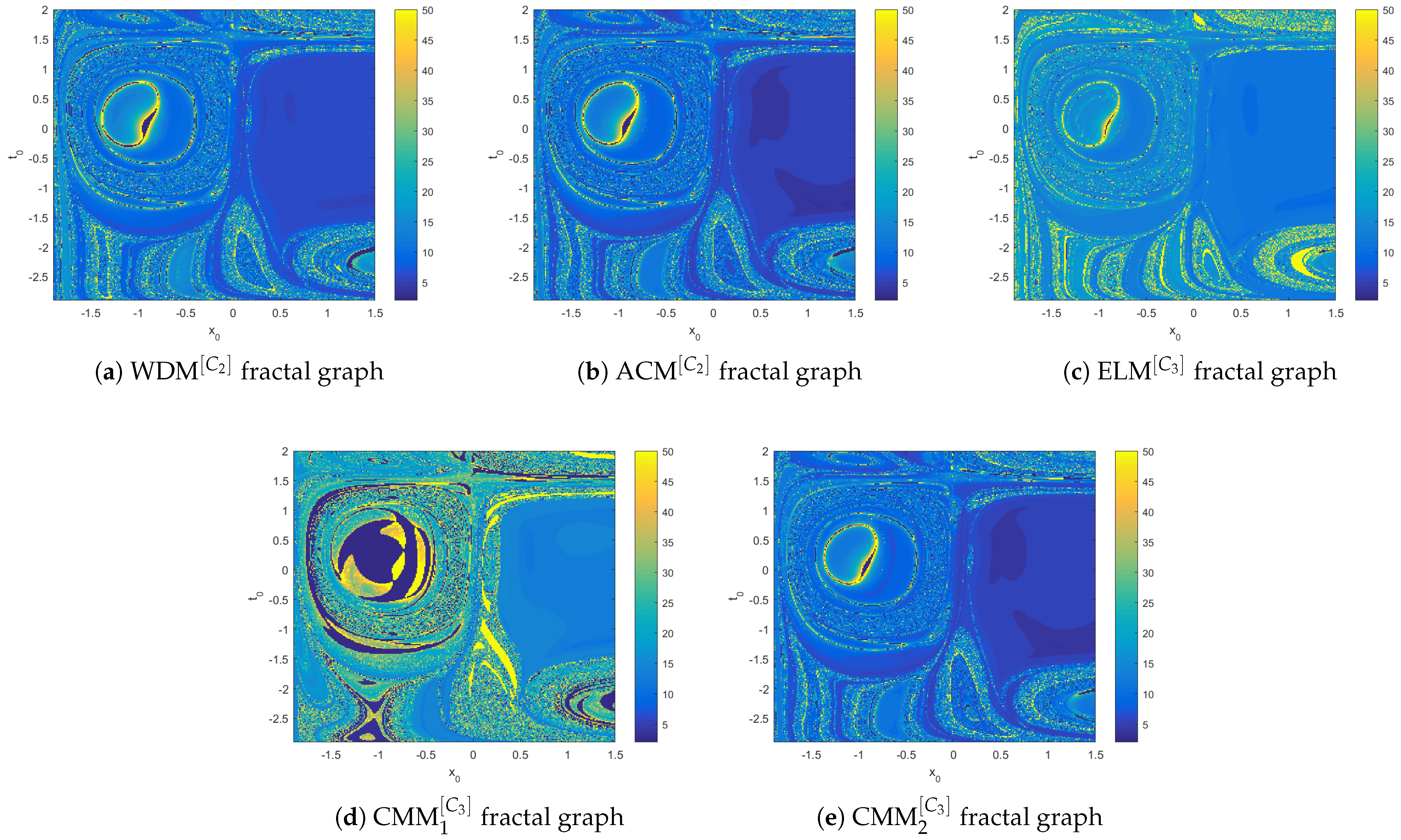
Fractal analysis: Fractal analysis is employed to identify favorable regions in the complex plane for initial guesses, thereby enabling faster and more reliable convergence of iterative schemes. Fractal patterns were generated for a system of $2\times 2$ nonlinear equations by considering a mesh of $2000\times 2000$ points over the complex domain $[-2,2]\times [-2,2]$. Each grid point corresponds to a distinct initial guess, and the assigned color indicates the root to which the iterative process converges. The resulting fractal boundaries highlight the method’s sensitivity near basin edges, thus providing insight into its global convergence behavior. The dense and well-structured basins of attraction confirm the robustness and stability of the technique. Moreover, the observed regularity of the patterns suggests limited chaotic behavior, further supporting the efficiency and reliability of the proposed scheme. To illustrate fractal analysis, we considered the nonlinear system

$$\left\{\begin{array}{c}{x}_1^2+x_2^2-e^{x_1}=0,\hfill \\ x_1{x}_2-e^{x_2}+1=0,\hfill \end{array}\right.$$

(50)

which has the approximate solutions $(x_1,x_2)\approx (-0.7035,0.0)$ and $(1.5407,1.3119)$.

The dynamical results in

Table 2. Numerical results of the dynamical analysis for solving (50) using different parallel iterative schemes. The metrics include the number of iterations (n), maximum error, percentage convergence (Per-C), arithmetic operations per iteration ($[+,-,\times ,÷]$), memory usage (MB), and elapsed time (s).

Method	n	Max-Error	Per-C	Ops [$+,-,\times ,÷$]	Memory (MB)	Elapsed Time (s)
${\mathrm{WDM}}^{\left[C_2\right]}$	20	$1.5\times {10}^{-3}$	$11.09\%$	19	87.657	87.657
${\mathrm{ACM}}^{\left[C_2\right]}$	9	$1.5\times {10}^{-7}$	$19.76\%$	65	55.657	55.657
${\mathrm{ELM}}^{\left[C_3\right]}$	12	$1.5\times {10}^{-15}$	$55.76\%$	53	47.764	47.764
${\mathrm{CMM}}_1^{\left[C_3\right]}$	8	$1.5\times {10}^{-18}$	$63.54\%$	54	45.567	45.567
${\mathrm{CMM}}_2^{\left[C_3\right]}$	7	$1.5\times {10}^{-35}$	$87.87\%$	36	34.453	34.453

and Figure 2a–e clearly demonstrate that the proposed method outperforms existing schemes in terms of convergence efficiency for solving CTFPDEs. It requires fewer iterations, uses less memory, and consequently reduces the overall computational cost. Moreover, Table 2 shows that the number of basic arithmetic operations, computed using Equation (48), is significantly smaller compared with competing approaches (${\mathrm{WDM}}^{\left[C_2\right]}$, ${\mathrm{ACM}}^{\left[C_2\right]}$, ${\mathrm{ELM}}^{\left[C_3\right]}$). The elapsed time required to generate the corresponding fractals is also markedly lower, confirming the speed advantage of our scheme. These results indicate that the method not only accelerates convergence but also preserves numerical stability across all test cases. In contrast, earlier approaches produce less uniform basins with broader chaotic regions, whereas our scheme yields well-defined convergence zones and improved robustness against divergence in challenging scenarios. Consequently, the newly developed methods ${\mathrm{CMM}}_1^{\left[C_3\right]}$–${\mathrm{CMM}}_2^{\left[C_3\right]}$ provide a reliable and effective framework for accurately solving (50).

3.1. Implementation of Methodology, Convergence Enhancement, and Result Visualization

This section introduces the numerical framework for solving fractional-order partial differential equations (PDEs) arising in biomedical engineering applications. The approach comprises three main stages: discretization of the fractional PDEs using the L1 scheme, solution of the resulting nonlinear system via a parallel root-finding algorithm, and convergence enhancement through initial vector sampling combined with adaptive stopping criteria. All simulations were performed in MATLAB R2023b (The MathWorks, Natick, MA, USA) on a PC equipped with an Intel Core i7 processor (Intel Corporation, Santa Clara, CA, USA) and 16 GB RAM. Convergence was defined as the residual norm falling below tol. The following performance metrics were recorded:

-

Iteration count;

-

Percentage convergence (P-Con);

-

Computational time (CPU seconds);

-

Memory usage (MB);

-

Percentage convergence under random initial values.

Discretization of CTFPDEs Using the L1 Scheme: Consider a CTFPDE defined on the spatial domain $[0,L]$ and time interval $[0,T]$, governed by a Caputo derivative of order $\alpha \in (0,1]$:

$$\left\{\begin{array}{c}{\displaystyle \frac{{\partial }^{\sigma }u}{\partial t^{\sigma }}}+{\displaystyle \frac{{\partial }^{2}u}{\partial x^2}}+{\displaystyle \frac{\partial u}{\partial x}}+u(x,t)=f(x,t),x\in [x^{\left[0\right]},x^{\left[n\right]}],t\in [t^{\left[0\right]},t^{\left[n\right]}],\hfill \\ u(x,0)=g_1\left(x\right),u(0,t)=g_2\left(t\right),u(L,t)=g_3\left(t\right).\hfill \end{array}\right.$$

(51)

Here, $\frac{{\partial }^{\sigma }u}{\partial t^{\sigma }}$ denotes the Caputo fractional derivative in time, $\frac{{\partial }^{2}u}{\partial x^2}$ represents diffusion, and $f(x,t)$ is a nonlinear source term. At discrete times $t_n=n\tau$, the Caputo derivative is approximated using the L1 scheme [48]:

$${\displaystyle \frac{{\partial }^{\sigma }u}{\partial t^{\sigma }}}\approx {\displaystyle \frac{1}{{\tau }^{\sigma }\Gamma (2-\sigma )}}\left[b_0{u}_i^n-{\displaystyle \sum _{k=1}^{n-1}}(b_{n-k-1}-b_{n-k})u_i^k-b_{n-1}{u}_i^0\right],$$

(52)

where $b_k={(k+1)}^{1-\sigma }-k^{1-\sigma }$. For compactness, this can be rewritten as

$${\displaystyle \frac{{\partial }^{\alpha }u}{\partial t^{\alpha }}}\approx {\displaystyle \frac{1}{{\tau }^{\sigma }\Gamma (2-\sigma )}}{\displaystyle \sum _{k=0}^n}{w}_k^{\left(n\right)}{u}_i^k,$$

(53)

with $w_0^{\left(n\right)}=b_0$, $w_k^{\left(n\right)}=b_{n-k-1}-b_{n-k}$ for $1\le k<n$, and $w_n^{\left(n\right)}=-b_{n-1}$. The spatial derivatives are approximated using standard central differences:

$${\displaystyle \frac{{\partial }^{2}u}{\partial x^2}}\approx {\displaystyle \frac{u_{i+1}^n-2u_i^n+u_{i-1}^n}{h^2}},{\displaystyle \frac{\partial u}{\partial x}}\approx {\displaystyle \frac{u_{i+1}^n-u_{i-1}^n}{2h}}.$$

(54)

Combining the temporal and spatial discretizations reduces the CTFPDE to a system of nonlinear algebraic equations at each time step:

$$\mathbf{F}\left(\mathbf{u}\right)=0,$$

(55)

where $\mathbf{u}\in {\mathbb{R}}^n$ denotes the vector of unknowns at time $t_n$.

Implementation: To solve $\mathbf{F}\left(\mathbf{u}\right)=0$, we employ a parallel iterative scheme designed to approximate all roots of the nonlinear system simultaneously. At iteration ℏ, the vector of approximations is

$${\mathbf{u}}^{[\hslash ]}={\left[{\mathbf{u}}_1^{[\hslash ]},\dots ,{\mathbf{u}}_n^{[\hslash ]}\right]}^t.$$

(56)

The scheme was implemented in two forms:

-

Criteria I: Element-wise scheme. Each solution component is updated independently in parallel:

$${\mathbf{u}}_i^{[\hslash +1]}={\mathbf{u}}_i^{[\hslash ]}-{\displaystyle \frac{\mathbf{F}\left({\mathbf{u}}_j^{[\hslash ]}\right)}{\underset{\begin{array}{c}t=1\\ t\ne i\end{array}}{\stackrel{n}{\Pi }}(u_i^{[\hslash ]},u_t^{[\hslash ]})}}.$$

(57)

-

Criteria II: Diagonalized scheme. The system is reformulated in matrix form and updated via

$${\mathbf{u}}_i^{[\hslash +1]}={\mathbf{u}}_i^{[\hslash ]}-{\displaystyle \frac{\mathbf{F}\left({\mathbf{u}}_j^{[\hslash ]}\right)}{\underset{\begin{array}{c}t=1\\ t\ne i\end{array}}{\stackrel{n}{\Pi }}\mathbf{G}({\mathbf{u}}_i^{[\hslash ]},{\mathbf{u}}_t^{[\hslash ]})}},$$

(58)

where $\mathbf{G}$ is a diagonal matrix that approximates a suitable operator to accelerate convergence.

-

Parallel implementation with MATLAB parfor. Both element-wise and diagonalized schemes were parallelized using MATLAB’s parfor construct, which distributes independent computations across multiple CPU cores. The main iteration loop was executed in parallel while ensuring data consistency and avoiding race conditions. Unlike OpenMP, MATLAB’s parfor replicates loop variables for each worker rather than automatically sharing memory, which may affect large-scale memory usage.

This parallelization reduces computational time while preserving the accuracy of the serial version. To quantify performance, we measured the serial CPU time (T_seri), parallel CPU time (T_para), and the speedup ratio, defined as

$$\mathrm{Speedup}\mathrm{Ratio}={\varphi }_{sp}={\displaystyle \frac{{\mathrm{T}}_{\mathrm{seri}}}{{\mathrm{T}}_{\mathrm{para}}}},$$

(59)

where T_seri corresponds to execution on a single core without MATLAB parfor, and T_para to execution on four cores with MATLAB parfor. Algorithm 1 and the flow chart in Figure 3 illustrate the complete implementation, including the computation of the COC and residual error for approximating the solution of (55). A higher speedup ratio indicates greater efficiency.

Acceleration of Convergence and Stopping Criteria. To enhance both convergence speed and reliability, the following steps were applied:

-

Initial Vector Sampling. For each numerical experiment, a single initial guess vector ${\mathbf{x}}_0$ is drawn randomly from a feasible domain, with magnitude close to ${10}^{-1}$ to improve the convergence rate. This unbiased initialization avoids selection bias and provides a fair evaluation of algorithmic robustness.

-

Selection Criterion. The iterative scheme is run on all sampled vectors, and the one yielding the highest accuracy is retained, measured by

$$∥{\mathbf{u}}_i^{[\hslash +1]}-{\mathbf{u}}_i^{[\hslash ]}∥<tol,$$

(60)

where $tol={10}^{-32}$. This high precision is achieved in MATLAB using the vpa function with digits = 64.

-

Stopping Criteria. The iteration is terminated once any of the following conditions is satisfied:

$${∥\mathbf{F}\left({\mathbf{u}}_i^{[\hslash ]}\right)∥}_2<tol,{∥\mathbf{F}\left({\mathbf{u}}_i^{[\hslash ]}\right)∥}_{\infty }<tol.$$

(61)

Visualization and Validation. The approximate solution ${\mathbf{u}}^{[\hslash ]}$ obtained from the iterative scheme is validated against exact or benchmark solutions. Both are plotted to illustrate the accuracy and convergence behavior. Algorithm 2 summarizes the complete approach, and Figure 3 presents the corresponding computational workflow.

3.2. Applications in Biomedical Engineering

Benchmark models play a central role in assessing the effectiveness and reliability of numerical methods for real-world biomedical problems. They provide a controlled setting in which computational performance can be tested under challenging conditions, such as highly nonlinear systems of equations. The inclusion of fractional-order parallel systems in these benchmarks allows researchers to evaluate accuracy, stability, and convergence when applied to medical and biological processes.

Algorithm 1 Parallel VPA Weierstrass method for solving fractional PDEs

Require:  Number of spatial nodes n, domain length L, time step $\tau$, fractional order $\alpha$, diffusion coefficient D, maximum number of iterations MaxIter, tolerance Tol, Weierstrass relaxation factor ${\lambda }_W$, small epsilon $\epsilon$ for VPA. Ensure:  Approximate solution $u_{\mathrm{approx}}$ at current time $t=\tau$, absolute error with respect to exact solution.   1: Initialize spatial grid: $x\leftarrow \mathrm{linspace}(0,L,n)$   2: Compute spatial step: $h\leftarrow x_2-x_1$   3: Initialize previous solution: $u_{\mathrm{prev}}\leftarrow \mathrm{vpa}(sin\left(\pi x\right))$   4: Define symbolic variables for unknowns: $u=\mathrm{sym}\left([u_1,u_2,\dots ,u_n]{,}^{\prime }rea{l}^{\prime }\right)$   5: Apply boundary conditions: $u_1=0$, $u_n=0$   6: Approximate Caputo derivative using L1 formula: $$L{1}_{\mathrm{Caputo}}={\displaystyle \frac{u-u_{\mathrm{prev}}}{{\tau }^{\alpha }\Gamma (2-\alpha )}}$$   7: Construct system of nonlinear equations for internal nodes $i=2$ to $n-1$: $$F_i=L{1}_{\mathrm{Caputo}}\left(i\right)-D{\displaystyle \frac{u_{i+1}-2u_i+u_{i-1}}{h^2}}$$   8: Reduce system to internal unknowns: $F_{\mathrm{red}}=[F_2,\dots ,F_{n-1}]$, $vars=[u_2,\dots ,u_{n-1}]$   9: Convert symbolic function to MATLAB function handle: $F_{\mathrm{func}}\left(vars\right)$ 10: Initialize guess for unknowns: $rootsApprox\leftarrow u_{\mathrm{prev}}(2:end-1)$ 11: Initialize new roots: $newRoots\leftarrow rootsApprox$ 12: for$iter=1$ to MaxIter do 13:       Store previous iteration: $tempRoots\leftarrow rootsApprox$ 14:       Parallel Weierstrass Step: 15:       for all $i=1$ to $n_{\mathrm{int}}$ in parallel (parfor loop) do 16:             Initialize product term: $prodTerm\leftarrow 1$ 17:             Evaluate system: $F_{\mathrm{val}}\leftarrow F_{\mathrm{func}}\left(rootsApprox\right)$ 18:             for $j=1$ to $n_{\mathrm{int}}$ do 19:                   if $j\ne i$ then 20:                         $diff\leftarrow rootsApprox\left(i\right)-rootsApprox\left(j\right)$ 21:                         if $\left|diff\right|<\epsilon$ then 22:                               $diff\leftarrow \epsilon$                                                                                            ▹avoid division by zero 23:                         end if 24:                         $prodTerm\leftarrow prodTerm·diff$ 25:                   end if 26:             end for 27:             Update root: $newRoots\left(i\right)\leftarrow rootsApprox\left(i\right)-{\lambda }_W·F_{\mathrm{val}}\left(i\right)/prodTerm$ 28:       end for 29:       Convergence Check: 30:       if $max\left(\right|newRoots-rootsApprox\left|\right)<\mathrm{Tol}$ then 31:             $rootsApprox\leftarrow newRoots$ 32:             break 33:       end if 34:       Update roots: $rootsApprox\leftarrow newRoots$ 35: end for 36: Construct full approximate solution: $u_{\mathrm{approx}}\leftarrow u_{\mathrm{prev}}$ 37: $u_{\mathrm{approx}}(2:end-1)\leftarrow rootsApprox$ 38: Compute exact solution using Mittag-Leffler function: $$u_{\mathrm{exact}}\left(i\right)=\mathrm{vpa}\left(e^{-x-t^{\sigma }}\right)$$ 39: Compute absolute error: $Error\leftarrow |u_{\mathrm{approx}}-u_{\mathrm{exact}}|$ 40: Output: $u_{\mathrm{approx}}$, $u_{\mathrm{exact}}$, $Error$ 41: Optional: Generate 3D plots for visual comparison between $u_{\mathrm{approx}}$ and $u_{\mathrm{exact}}$ along with error graph.

Algorithm 2 Parallel scheme for solving (55) using MATLAB parfor parallelization on multiple cores

1: Input: Nonlinear system $F\left(x\right)$, initial guesses $X^{\left(0\right)}=[x_1^{\left(0\right)},x_2^{\left(0\right)},\dots ,x_n^{\left(0\right)}]$ 2: Parameters: Tolerance $\epsilon$, maximum number of iterations $N_{max}$, version (pointwise or diagonalized) 3: Set $k\leftarrow 0$ 4: while  $k<N_{max}$  do 5:       Compute $F\left(X^{\left(k\right)}\right)=[f_1\left(x^{\left(k\right)}\right),f_2\left(x^{\left(k\right)}\right),\dots ,f_n\left(x^{\left(k\right)}\right)]$ 6:       if pointwise version then 7:             for $i=1$ to n do 8:                   Compute the product $P_i={\prod }_{j\ne i}(x_i^{\left(k\right)}-x_j^{\left(k\right)})$ 9:                   Update $x_i^{(k+1)}=x_i^{\left(k\right)}-{\displaystyle \frac{f_i\left(x_i^{\left(k\right)}\right)}{P_i}}$ 10:             end for 11:       else if diagonalized version then 12:             Construct diagonal matrix D with $D_{ii}={\prod }_{j\ne i}(x_i^{\left(k\right)}-x_j^{\left(k\right)})$ 13:             $X^{(k+1)}=X^{\left(k\right)}-D^{-1}F\left(X^{\left(k\right)}\right)$ 14:       end if 15:       if $\parallel X^{(k+1)}-X^{\left(k\right)}\parallel <\epsilon$ then 16:             Converged: Return $X^{(k+1)}$ 17:       end if 18:       $k\leftarrow k+1$ 19: end while 20: Return: $X^{(k+1)}$, "Maximum iterations reached"

3.2.1. Drug Diffusion in Tissue with Nonlinear Reaction [49]

Drug diffusion in tissue with nonlinear reactions is a fundamental process in biomedical engineering, pharmacology, and treatment design. In therapeutic applications such as targeted drug delivery, cancer therapy, and tissue engineering, drugs diffuse through biological tissue while simultaneously undergoing metabolic reactions, receptor binding, or cellular uptake. These reactions are often nonlinear due to saturation effects, cooperative binding, or enzymatic kinetics (e.g., Michaelis–Menten).

To capture these dynamics, mathematical modeling is essential for describing the spatiotemporal evolution of drug concentration, predicting therapeutic efficacy, and minimizing side effects. The governing equations typically couple diffusion—the passive transport of drug molecules through the extracellular matrix—with nonlinear reaction terms representing biochemical interactions. Incorporating fractional-order derivatives enables the model to capture anomalous diffusion observed in heterogeneous tissues, where transport deviates from classical Fickian behavior due to structural barriers and memory effects.

Such models, when implemented numerically, enable realistic simulation of drug–tissue interactions, optimization of dosing strategies, and the design of treatment protocols tailored to patient-specific conditions.

A time-fractional reaction–diffusion equation is used to model the spatiotemporal evolution of the drug concentration $u(x,t)$ in a one-dimensional tissue segment $x\in [0,L]$ [50]:

$$\left\{\begin{array}{cc}{\displaystyle \frac{{\partial }^{\sigma }u}{\partial t^{\sigma }}=\frac{{\partial }^{2}u}{\partial x^2}+\frac{\partial u}{\partial x}+u+\lambda u^2(1-u)+f(x,t),}\hfill & x\in [x^{\left[0\right]},x^{\left[n\right]}],t\in [t^{\left[0\right]},t^{\left[n\right]}],\hfill \\ u(x,0)=e^{-x},\hfill \\ u(0,t)=e^{-t^{\sigma }},u(2,t)=e^{-2-t^{\sigma }},\hfill \end{array}\right.$$

(62)

where the source term $f(x,t)$ is chosen such that the exact solution

$$u(x,t)=e^{-x-t^{\sigma }}$$

(63)

satisfies the PDE exactly. In particular, the source term is defined as

$$f(x,t)=\lambda \left(e^{-3x-3t^{\sigma }}-e^{-2x-2t^{\sigma }}\right)-e^{-x-t^{\sigma }}+Q_1^{[\ast ]},$$

(64)

where

$$Q_1^{[\ast ]}={\Gamma }^{-1}(-\sigma ){\int }_0^t{\tau }^{\sigma -2}{e}^{-x-{\tau }^{\sigma }}{(t-\tau )}^{-\sigma }d\tau .$$

Remark 1. 

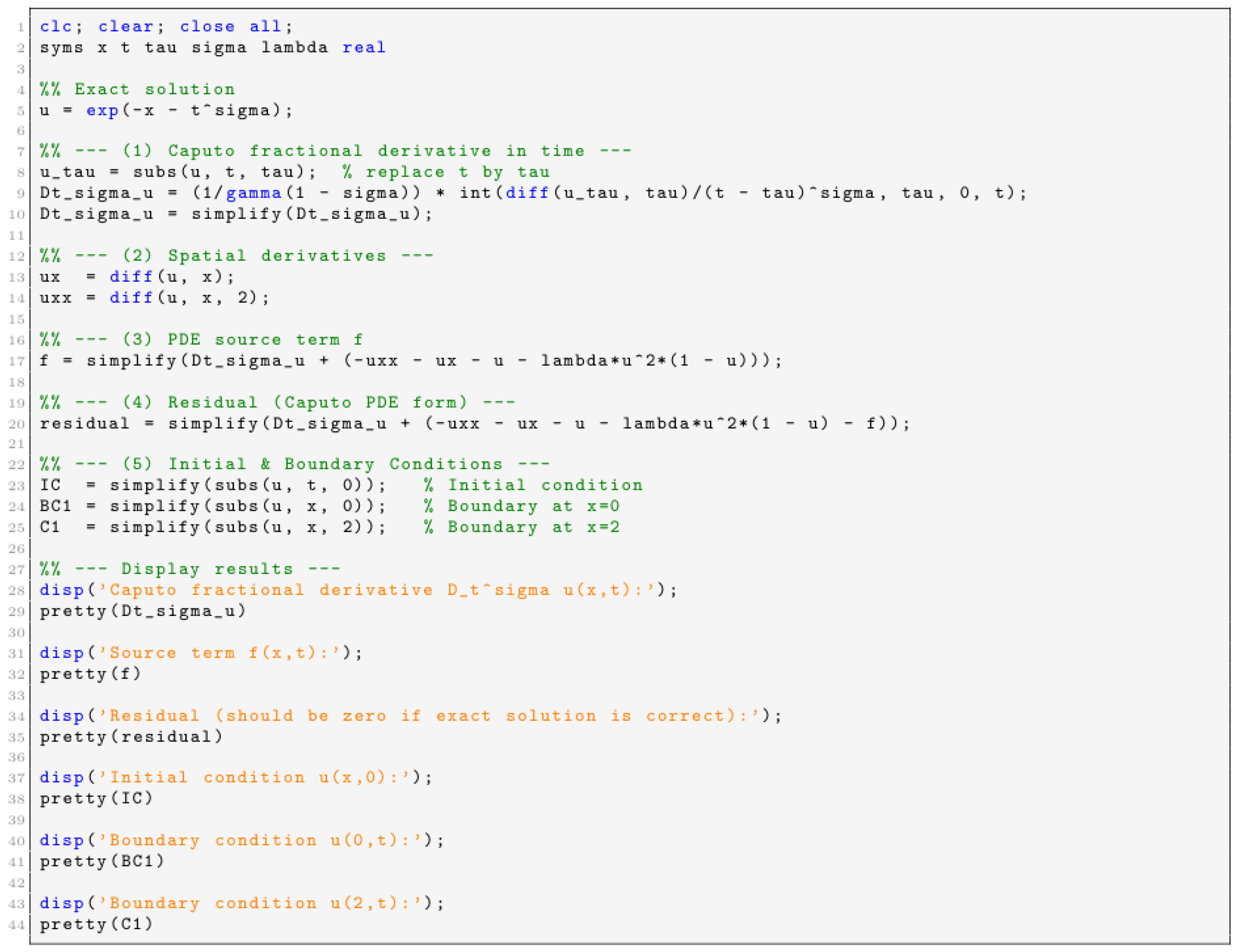
The exact solution (81) is consistent with the initial and boundary conditions, while the source term (64) guarantees that the PDE residual vanishes. This construction provides a valid and unbiased benchmark for error assessment (see MATLAB symbolic script in Appendix A.1, Figure A1).

The problem setup is characterized as follows:

• Spatial domain: $x\in [0,2]$, discretized into N intervals with spacing $h=L/N$.
• Time domain: $t\in [0,1]$, discretized into M intervals with spacing $\tau =T/M$.
• Grid nodes: $x_i=ih,i=0,\dots ,N$, and $t_n=n\tau ,n=0,\dots ,M$.
• Unknown: $u_i^n\approx u(x_i,t_n)$.

The Caputo fractional PDE is discretized in time using the L1 scheme:

$${\displaystyle \frac{{\partial }^{\sigma }u}{\partial t^{\sigma }}}\approx {\displaystyle \frac{1}{{\tau }^{\sigma }\Gamma (2-\sigma )}}\left[b_0{u}_i^n-{\displaystyle \sum _{k=1}^{n-1}}(b_{n-k-1}-b_{n-k})u_i^k-b_{n-1}{u}_i^0\right],$$

(65)

where $b_k={(k+1)}^{1-\sigma }-k^{1-\sigma }$. For convenience, this expression can be rewritten as

$${\displaystyle \frac{{\partial }^{\sigma }u}{\partial t^{\sigma }}}\approx {\displaystyle \frac{1}{{\tau }^{\sigma }\Gamma (2-\sigma )}}{\displaystyle \sum _{k=0}^n}{w}_k^{\left(n\right)}{u}_i^k,$$

(66)

with weights defined as $w_0^{\left(n\right)}=b_0$, $w_k^{\left(n\right)}=b_{n-k-1}-b_{n-k}$ for $1\le k<n$, and $w_n^{\left(n\right)}=-b_{n-1}$. The spatial derivatives are discretized using finite differences:

$${\displaystyle \frac{{\partial }^{2}u}{\partial x^2}}\approx {\displaystyle \frac{u_{i+1}^n-2u_i^n+u_{i-1}^n}{h^2}},$$

(67)

$${\displaystyle \frac{\partial u}{\partial x}}\approx {\displaystyle \frac{u_{i+1}^n-u_{i-1}^n}{2h}}.$$

(68)

By substituting (66)–(68) into (62), the fully discretized system at each spatial point can be written as

$${\displaystyle \frac{1}{{\tau }^{\sigma }\Gamma (2-\sigma )}}{\displaystyle \sum _{k=1}^{n-1}}{w}_k^{\left(n\right)}{u}_i^k={\displaystyle \frac{u_{i+1}^n-2u_i^n+u_{i-1}^n}{h^2}}+{\displaystyle \frac{u_{i+1}^n-u_{i-1}^n}{2h}}+u_i^n+\lambda {\left(u_i^n\right)}^2\left(1-u_i^n\right)+f_i^n,$$

(69)

where

$$f_i^n=f(x_i,t^n)=\lambda exp(-2x_i-2t_n^{\alpha })\left(1-exp(-x_i-t_n^{\sigma })\right).$$

(70)

In matrix form, the system can be expressed as

$${\displaystyle \frac{1}{{\tau }^{\sigma }\Gamma (2-\sigma )}}{\displaystyle \sum _{k=1}^{n-1}}{w}_k^{\left(n\right)}{\mathbf{u}}^k={\mathbf{D}}_1{\mathbf{u}}^n+{\mathbf{D}}_2{\mathbf{u}}^n+{\mathbf{u}}^n+\lambda {\left({\mathbf{u}}^n\right)}^2\odot (1-{\mathbf{u}}^n)+{\mathbf{f}}^n,$$

(71)

where

• ⊙ denotes element-wise operations;
• ${\mathbf{f}}^n={[f_1^n,f_2^n,\dots ,f_{N-1}^n]}^T$.

The discrete differential operators are defined as

$${\mathbf{D}}_1={\displaystyle \frac{1}{h^2}}\mathrm{tridig}(1,-2,1)={\displaystyle \frac{1}{h^2}}\left[\begin{array}{ccccc}-2& 1& 0& \dots & 0\\ 1& -2& 1& \dots & 0\\ 0& \ddots & \ddots & \ddots & 0\\ 0& \dots & 1& -2& 1\\ 0& \dots & 0& 1& -2\end{array}\right],$$

(72)

and

$${\mathbf{D}}_2={\displaystyle \frac{1}{2h}}\mathrm{tridig}(-1,0,1)={\displaystyle \frac{1}{2h}}\left[\begin{array}{ccccc}0& 1& 0& \dots & 0\\ -1& 0& 1& \dots & 0\\ 0& \ddots & \ddots & \ddots & 0\\ 0& \dots & -1& 0& 1\\ 0& \dots & 0& -1& 0\end{array}\right].$$

(73)

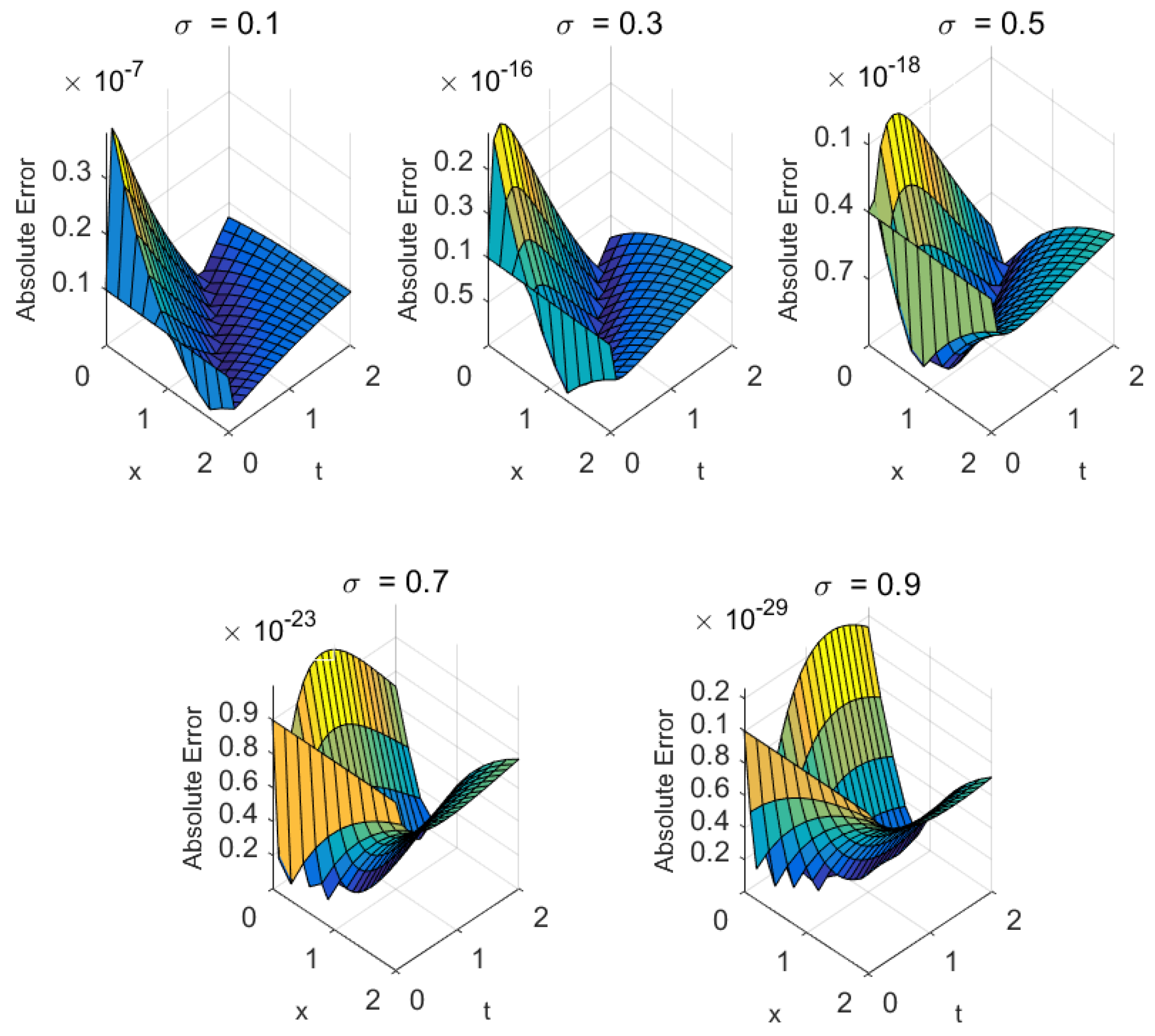
The numerical results obtained with the proposed parallel scheme ${\mathrm{CMM}}_1^{\left[C_3\right]}$ for solving the considered problem are summarized in

Table 3. Maximum error norms of parallel scheme ${\mathrm{CMM}}_2^{\left[C_3\right]}$ without MATLAB parfor for different fractional orders $\sigma$. Results are reported for varying grid sizes.

Grid Points	${\parallel .\parallel }_2$-Norm	${\parallel .\parallel }_{\mathit{\infty }}$-Norm	CPU Time (s)
	$\sigma =0.1$
30, 50	$8.543\times {10}^{-5}$	$5.034\times {10}^{-6}$	0.056
60, 90	$5.024\times {10}^{-6}$	$5.053\times {10}^{-6}$	0.120
120, 180	$2.753\times {10}^{-6}$	$1.235\times {10}^{-7}$	0.250
	$\sigma =0.3$
30, 50	$9.541\times {10}^{-16}$	$5.376\times {10}^{-11}$	0.060
60, 90	$5.540\times {10}^{-13}$	$1.897\times {10}^{-13}$	0.125
120, 180	$1.587\times {10}^{-12}$	$8.760\times {10}^{-15}$	0.260
	$\sigma =0.5$
30, 50	$7.565\times {10}^{-17 †}$	$1.008\times {10}^{-15}$	0.065
60, 90	$1.554\times {10}^{-18 †}$	$5.744\times {10}^{-17 †}$	0.130
120, 180	$3.577\times {10}^{-17 †}$	$9.898\times {10}^{-16 †}$	0.270
	$\sigma =0.7$
30, 50	$5.340\times {10}^{-22 †}$	$1.744\times {10}^{-21 †}$	0.070
60, 90	$6.589\times {10}^{-23 †}$	$2.395\times {10}^{-22 †}$	0.135
120, 180	$7.550\times {10}^{-21 †}$	$7.890\times {10}^{-21 †}$	0.280
	$\sigma =0.9$
30, 50	$3.567\times {10}^{-26 †}$	$1.535\times {10}^{-29 †}$	0.075
60, 90	$4.776\times {10}^{-27 †}$	$3.876\times {10}^{-27 †}$	0.145
120, 180	$1.755\times {10}^{-27 †}$	$4.890\times {10}^{-26 †}$	0.301

^† All computations were performed using MATLAB VPA with digits = 64 and a numerical tolerance of 10⁻³⁰.

. In these simulations, the initial guess vectors were chosen sufficiently close to the exact solution (within a tolerance of $0.01$) to ensure rapid convergence and to avoid the instability associated with poor initial approximations. Table 3 reports the computed solutions for different spatial grid sizes and fractional-order parameters $\sigma$, demonstrating the robustness and accuracy of the scheme across varying problem scales and fractional dynamics. Figure 4 and Figure 5 display the exact and approximate solutions of (71), together with the corresponding absolute errors.

To provide a comprehensive performance evaluation,

Table 4. Error comparison between parallel schemes for solving (71) with $\sigma \approx 1$, under Criterion I and Criterion II, without MATLAB parfor.

Metric	${\mathrm{WDM}}^{\left[{\mathit{C}}_2\right]}$	${\mathrm{ACM}}^{\left[{\mathit{C}}_2\right]}$	${\mathrm{ELM}}^{\left[{\mathit{C}}_3\right]}$	${\mathrm{CMM}}_1^{\left[{\mathit{C}}_3\right]}$	${\mathrm{CMM}}_2^{\left[{\mathit{C}}_3\right]}$
		Criterion I
${\parallel .\parallel }_2$-norm	$1.10\times {10}^{-8}$	$1.35\times {10}^{-8}$	$4.80\times {10}^{-9}$	$1.89\times {10}^{-19 †}$	$1.39\times {10}^{-27 †}$
${\parallel .\parallel }_{\infty }$-norm	$4.51\times {10}^{-5}$	$6.72\times {10}^{-6}$	$5.84\times {10}^{-9}$	$7.06\times {10}^{-23 †}$	$9.44\times {10}^{-24 †}$
		Criterion II
${\parallel .\parallel }_2$-norm	$5.70\times {10}^{-6}$	$3.00\times {10}^{-8}$	$1.65\times {10}^{-7}$	$1.50\times {10}^{-21 †}$	$1.04\times {10}^{-25 †}$
${\parallel .\parallel }_{\infty }$-norm	$9.41\times {10}^{-6}$	$5.35\times {10}^{-7}$	$3.00\times {10}^{-10}$	$1.14\times {10}^{-23 †}$	$4.10\times {10}^{-26 †}$

^† All computations were performed using MATLAB variable precision arithmetic (VPA) with digits = 64 and a numerical tolerance of ${10}^{-30}$.

compares the proposed approach with other well-established methods from the literature for selected grid sizes ($120,180$) and fractional parameter $\sigma \approx 1$, thus assessing performance in the near-integer order regime. This comparative analysis highlights the efficiency, precision, and computational advantages of the ${\mathrm{CMM}}_1^{\left[C_3\right]}$ scheme, confirming its suitability for high-accuracy fractional-order simulations in practical applications.

Table 4 presents the numerical results obtained with the proposed method, where the initial approximations were deliberately chosen close to the exact solutions to ensure stable and rapid convergence. The results confirm the accuracy and efficiency of the method across different test configurations. A comparative analysis with state-of-the-art parallel iterative schemes—${\mathrm{WDM}}^{\left[C_2\right]}$, ${\mathrm{ACM}}^{\left[C_2\right]}$, and  ${\mathrm{ELM}}^{\left[C_3\right]}$—shows that the proposed ${\mathrm{CMM}}_1^{\left[C_3\right]}$–${\mathrm{CMM}}_2^{\left[C_3\right]}$ approaches consistently achieve substantially lower residual errors. This improvement underscores the enhanced stability and convergence properties of the scheme, making it a strong candidate for high-precision computations in nonlinear systems. The overall performance of the parallel schemes is summarized in

Table 5. Overall performance of parallel schemes for solving (71) without MATLAB parfor. Here, “Basic Ops” denotes the number of basic arithmetic operations ($+,-,\times ,÷$).

Metric	Iter. (n)	Max Error	Conv. (%)	Basic Ops	Memory (MB)	COC
${\mathrm{WDM}}^{\left[C_2\right]}$	13	$4.51\times {10}^{-5}$	11.09	47	87.657	2.0014
${\mathrm{ACM}}^{\left[C_2\right]}$	13	$6.72\times {10}^{-6}$	19.76	51	55.657	2.0346
${\mathrm{ELM}}^{\left[C_3\right]}$	11	$1.65\times {10}^{-7}$	55.76	50	47.764	1.9993
${\mathrm{CMM}}_1^{\left[C_3\right]}$	9	$1.89\times {10}^{-11}$	63.54	54	45.567	3.1164
${\mathrm{CMM}}_2^{\left[C_3\right]}$	9	$4.10\times {10}^{-12}$	87.87	36	34.453	3.0087

, for a fractional parameter $\sigma =0.9$ and grid sizes of 120 and 180.

Table 5 demonstrates that, across all key performance metrics—number of iterations, maximum error, percentage convergence, total arithmetic operations, memory usage, and computational order of convergence (COC)—the proposed ${\mathrm{CMM}}_1^{\left[C_3\right]}$–${\mathrm{CMM}}_2^{\left[C_3\right]}$ methods significantly outperform the existing approaches ${\mathrm{WDM}}^{\left[C_2\right]}$, ${\mathrm{ACM}}^{\left[C_2\right]}$, and ${\mathrm{ELM}}^{\left[C_3\right]}$. Random initial guess vectors were used to analyze the global convergence of parallel techniques for solving (71). This procedure ensured accuracy up to two decimal places relative to the exact solution. The adaptive selection process markedly improved robustness and efficiency across a wide range of problem instances. The random initial guess vectors employed for the bio-heat problem are reported in

Table 6. Discretization details of the bio-heat transfer problem used for generating random initial guess vectors.

Application	Domain $(\mathit{x},\mathit{t})$	Recorded Variables	Approx. Data Size
Bio-heat transfer	$x\in [0,1],t\in [0,1]$	$x_i,t^k,u_{i-1}^{k-1},u_i^{k-1},u_{i+1}^{k-1}$	$\sim M\times N$

and

Table 7. Example of a random initial guess vector drawn from 100 MATLAB-generated test samples.

${\mathit{x}}_{\mathit{i}}$	${\mathit{t}}^{\mathit{k}}$	${\mathit{u}}_{\mathit{i}-1}^{\mathit{k}-1}$	${\mathit{u}}_{\mathit{i}}^{\mathit{k}-1}$	${\mathit{u}}_{\mathit{i}+1}^{\mathit{k}-1}$	${\mathit{u}}_{\mathit{i}}^{\mathit{k}}$
0.03333	0.02000	0.98020	0.96722	0.95444	0.96724
0.73333	0.04000	0.47924	0.47237	0.46561	0.47240
0.46667	0.08000	0.62101	0.61653	0.61208	0.61655
⋮ (remaining entries omitted)

.

The results of the adaptive self-adjustment of initial guess values, as described in Algorithm 1, are presented in

Table 8. Maximum error outcomes of parallel schemes ${\mathrm{CMM}}_1^{\left[C_3\right]}$–${\mathrm{CMM}}_2^{\left[C_3\right]}$ implemented via MATLAB parfor for solving (71).

$\mathit{\sigma }$	0.1	0.3	0.5	0.7	0.9	Mem U
		Using Criterion I
${\mathrm{CMM}}_1^{\left[C_3\right]}$	$1.09\times {10}^{-3}$	$0.67\times {10}^{-7}$	$2.43\times {10}^{-11}$	$0.16\times {10}^{-15}$	$2.52\times {10}^{-19 †}$	$57.155$
${\mathrm{CMM}}_2^{\left[C_3\right]}$	$3.10\times {10}^{-4}$	$5.67\times {10}^{-6}$	$0.45\times {10}^{-10}$	$9.05\times {10}^{-13}$	$0.41\times {10}^{-17 †}$	$56.007$
		Using Criterion II
${\mathrm{CMM}}_1^{\left[C_3\right]}$	$0.09\times {10}^{-3}$	$2.76\times {10}^{-5}$	$3.07\times {10}^{-9}$	$0.69\times {10}^{-11}$	$1.17\times {10}^{-16 †}$	$56.644$
${\mathrm{CMM}}_2^{\left[C_3\right]}$	$6.25\times {10}^{-5}$	$5.13\times {10}^{-7}$	$4.55\times {10}^{-14}$	$1.13\times {10}^{-19 †}$	$1.67\times {10}^{-21 †}$	$49.177$

^† All computations were performed using MATLAB variable precision arithmetic (VPA) with digits = 64, employing a numerical tolerance of 10⁻³⁰.

for both Criteria I and II.

Table 8 demonstrates the accuracy of the proposed schemes in solving CTFPDEs for different parameter values. For grid sizes of 120 and 180, the methods ${\mathrm{CMM}}_1^{\left[C_3\right]}$–${\mathrm{CMM}}_2^{\left[C_3\right]}$ outperform earlier approaches (${\mathrm{WDM}}^{\left[C_2\right]}$, ${\mathrm{ACM}}^{\left[C_2\right]}$, and ${\mathrm{ELM}}^{\left[C_3\right]}$) in terms of accuracy. Table 8 also reports the overall consistency analysis, performed using randomly generated initial values. Furthermore, the results in

Table 9. Consistency analysis using random initial guess vectors for parallel schemes ${\mathrm{CMM}}_1^{\left[C_3\right]}$–${\mathrm{CMM}}_2^{\left[C_3\right]}$ implemented with MATLAB parfor for solving (71).

Metric	Average Iterations	COC	CPU Time (s)	Percentage Convergence	Memory Usage (MB)
Using Criterion I
${\mathrm{CMM}}_1^{\left[C_3\right]}$	17	$4.0975$	$1.3425$	$76.77\%$	$41.14$
${\mathrm{CMM}}_2^{\left[C_3\right]}$	16	$6.0126$	$1.6766$	$97.56\%$	$46.60$
Using Criterion II
${\mathrm{CMM}}_1^{\left[C_3\right]}$	15	$6.0126$	$1.6766$	$97.56\%$	$47.12$
${\mathrm{CMM}}_2^{\left[C_3\right]}$	16	$6.0126$	$1.6766$	$97.56\%$	$46.40$

confirm that the proposed method achieves higher accuracy and stability than existing schemes. Across all evaluation metrics—including the average number of iterations, computational time (seconds), percentage convergence, and memory utilization—our approach consistently outperforms the alternatives under both Criterion I and Criterion II.

The results obtained from the MATLAB parfor parallel implementation are reported in

Table 10. Outcomes of parallel schemes ${\mathrm{CMM}}_1^{\left[C_3\right]}$–${\mathrm{CMM}}_2^{\left[C_3\right]}$ implemented with MATLAB parfor for solving (71). Reported errors are capped at double-precision limits; see footnote for full VPA residuals.

Metric	${\mathit{T}}_{\mathbf{seri}}$ (s)	${\mathit{T}}_{\mathbf{para}}$ (s)	${\mathit{\varphi }}_{\mathbf{speed}}$	Maximum Error	Percentage Convergence	Memory Usage (MB)
Using Criterion I
${\mathrm{CMM}}_1^{\left[C_3\right]}$	1.45	0.52	2.79	$\le 2.12\times {10}^{-17 †}$	86.01%	35.03
${\mathrm{CMM}}_2^{\left[C_3\right]}$	3.87	1.35	2.87	$\le 2.22\times {10}^{-17 †}$	87.56%	36.11
Using Criterion II
${\mathrm{CMM}}_1^{\left[C_3\right]}$	8.59	2.95	2.91	$\le 2.22\times {10}^{-16 †}$	91.57%	29.11
${\mathrm{CMM}}_2^{\left[C_3\right]}$	9.14	3.10	2.95	$\le 2.22\times {10}^{-16 †}$	92.12%	23.12

^† All computations used MATLAB VPA (digits = 64). Raw VPA residuals for the maximum error were $2.13\times {10}^{-28}$, $9.85\times {10}^{-29}$ (Criterion I) and $1.573\times {10}^{-27}$, $1.567\times {10}^{-30}$ (Criterion II). For consistent reporting across floating-point environments, the displayed values are $min\{\mathrm{VPA}\mathrm{residual},2.22\times {10}^{-16}\}$, ensuring comparability with IEEE double precision.

.

The proposed MATLAB parfor-based parallelization of the schemes achieves significant acceleration across all test cases. As shown in Table 10, the parallel implementation attains a speedup ratio of $2.95$–$3\times$ on a four-core machine, indicating efficient utilization of the available cores. Notably, the maximum error and percentage convergence remain consistent with the serial approach, confirming that accuracy is preserved. Moreover, memory usage shows slight improvements due to optimized data handling within the parallel loops.

Physical Behavior of Drug Diffusion in Tissue with Nonlinear Reaction Model.

In the drug diffusion model, the fractional-order time derivative governs the temporal evolution of concentration, while the nonlinear reaction term regulates saturation effects. To ensure both accuracy and computational efficiency, numerical parameters were selected according to these structural properties, including time step and spatial discretization.

• Step size and tolerance were chosen to balance accuracy and convergence.
• Numerical results showed that the proposed approach preserved the model’s physical behavior over time and space.
• The interaction between fractional order, nonlinearity, and numerical discretization directly affected computational cost and convergence speed.

3.2.2. Brain Signal Propagation with Nonlinear Blood Flow Effects [51]

Brain signal propagation with nonlinear blood flow effects is an emerging interdisciplinary research area at the intersection of neuroscience, biofluid mechanics, and mathematical physics. Neural signal transmission is governed by complex electrochemical processes along neuronal pathways, while cerebral blood flow delivers the oxygen and nutrients required for proper neuronal activity. The coupling between vascular hemodynamics, neuronal firing dynamics, and ionic transport produces inherently nonlinear interactions—both under physiological conditions and more prominently in pathological states such as stroke, epilepsy, or traumatic brain injury.

From a mathematical perspective, these interactions are often modeled by coupling nonlinear reaction–diffusion or fractional-order cable equations (describing axonal signal diffusion and membrane potential dynamics) with Navier–Stokes-type or Darcy–Forchheimer equations (representing nonlinear blood flow through microvasculature). Additional nonlinearities may arise from synaptic saturation, threshold-based action potentials, or rheological effects of blood such as shear-dependent viscosity. Fractional calculus has gained increasing importance in this context, as it captures memory effects in vascular and neural components, including anomalous diffusion in the extracellular space and delayed hemodynamic responses.

The resulting coupled models enable the simulation of realistic patterns of brain signal propagation, the prediction of delays induced by impaired blood flow, and the evaluation of therapeutic interventions such as modulation of neurovascular coupling. By integrating electrophysiological and hemodynamic processes into a unified mathematical framework, these models provide deeper insight into brain function and pathology, supporting advances in brain–computer interfaces, diagnostic imaging, and targeted therapeutic strategies [52].

Let $u(x,t)$ denote the neural field (e.g., membrane potential, averaged activity, or signal amplitude) on a one-dimensional tissue domain $x\in [0,L]$. To capture anomalous temporal dynamics, we employ a Caputo fractional derivative of order $0<\sigma \le 1$. The governing FPDE is given by

$$\left\{\begin{array}{cc}{\displaystyle \frac{{\partial }^{\sigma }u}{\partial t^{\sigma }}=v_1^{[\ast ]}\frac{{\partial }^{2}u}{\partial x^2}+v_2^{[\ast ]}\frac{\partial u}{\partial x}+u(x,t)+f(x,t),}\hfill & x\in [0,2],t\in [0,1],\hfill \\ u(x,0)=2.09+sin\left(\pi x\right),\hfill \\ u(0,t)=0,u(2,t)=2(t^{\sigma }+1.09)+sin\left(2\pi \right),\hfill \end{array}\right.$$

(74)

where the source term $f(x,t)$ is chosen such that the exact solution

$$u(x,t)=\left(2t^{\sigma }+2.18\right)+sin\left(\pi x\right)$$

(75)

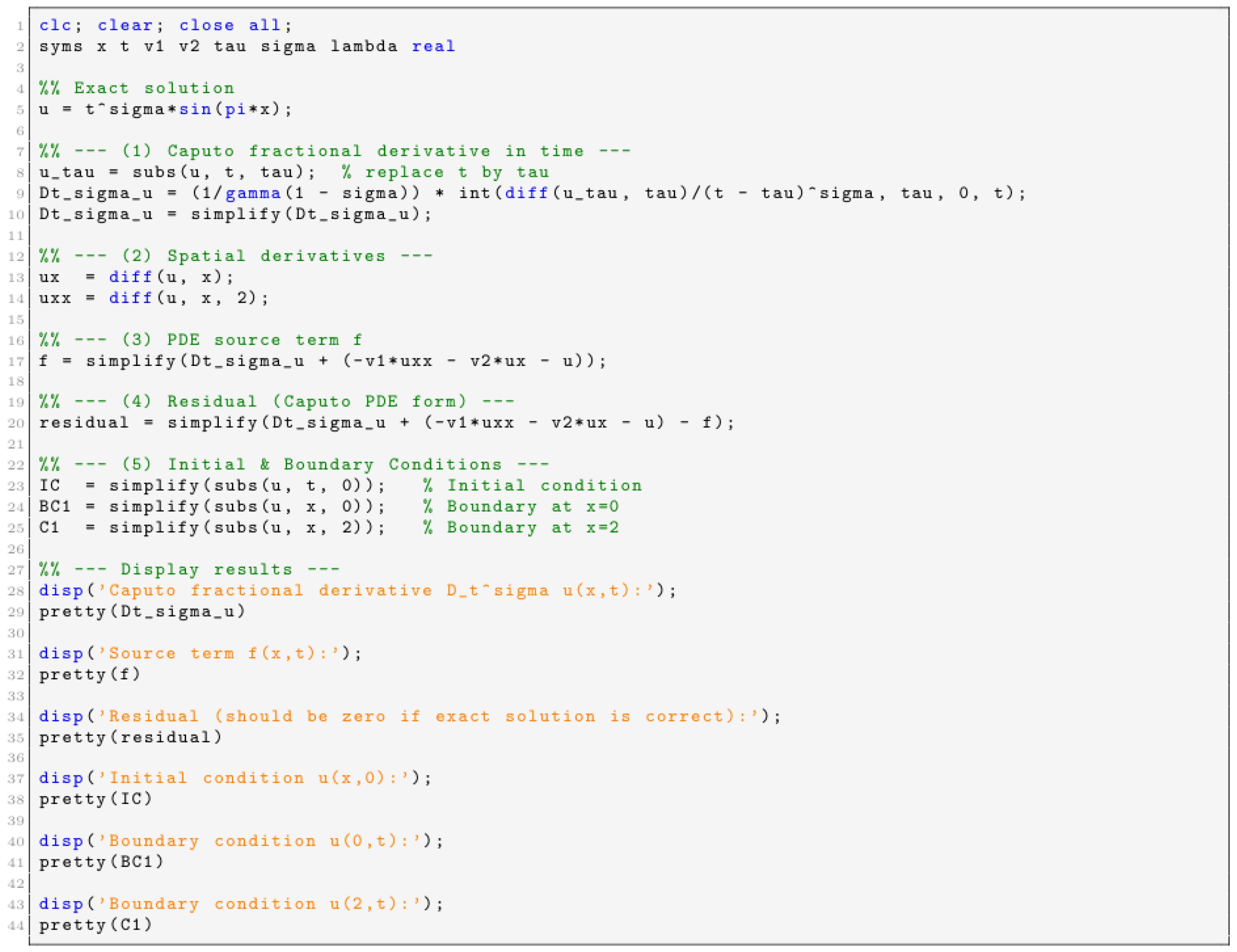
satisfies the PDE exactly (see MATLAB symbolic script in Appendix A.2, Figure A2). In particular, the source term is defined as

$$f(x,t)=t^{\sigma }\left(({\pi }^2{v}_1^{[\ast ]}-1)sin\left(\pi x\right)-\pi v_2^{[\ast ]}cos\left(\pi x\right)\right)-sin\left(\pi x\right)Q_2^{[\ast ]},$$

(76)

where

$$Q_2^{[\ast ]}={\Gamma }^{-1}(-\sigma ){\int }_0^t{\tau }^{\sigma -2}{(t-\tau )}^{-\sigma }d\tau .$$

Model parameters and discretization:

• $v_1^{[\ast ]}$: effective diffusion coefficient of the electrical signal (axonal/dendritic spread).
• $v_2^{[\ast ]}$: advective drift term (typically small; set $v_2^{[\ast ]}=0$ unless modeling directed flow).
• $f(x,t)$: external source term.
• Spatial domain: $x\in [0,2]$, discretized into N intervals with spacing $h=L/N$.
• Temporal domain: $t\in [0,1]$, discretized into M intervals with spacing $\tau =T/M$.
• Grid nodes: $x_i=ih$, $i=0,\dots ,N$; $t_n=n\tau$, $n=0,\dots ,M$.
• Unknowns: $u_i^n\approx u(x_i,t_n)$.

Using approximations (66)–(68) in (74), we obtain the following nonlinear system of equations:

$${\displaystyle \frac{1}{\tau \Gamma (2-\sigma )}}{\displaystyle \sum _{k=1}^{n-1}}{w}_k^{\left(n\right)}{u}_i^k={\displaystyle \frac{u_{i+1}^n-2u_i^n+u_{i-1}^n}{h^2}}+{\displaystyle \frac{u_{i+1}^n-u_{i-1}^n}{2h}}+u_i^n+f_i^n,$$

(77)

where

$$f_i^n=f(x_i,t^n)=sin\left(u_i^n\right).$$

(78)

In matrix form, the system can be expressed as

$${\displaystyle \frac{1}{\tau \Gamma (2-\sigma )}}{\displaystyle \sum _{k=1}^{n-1}}{w}_k^{\left(n\right)}{\mathbf{u}}^k={\mathbf{D}}_1{\mathbf{u}}^n+{\mathbf{D}}_2{\mathbf{u}}^n+{\mathbf{u}}^n+{\mathbf{f}}^n,$$

(79)

where

• ⊙ denotes element-wise operations;
• ${\mathbf{f}}^n={[f_1^n,f_2^n,\dots ,f_{N-1}^n]}^T$;
• ${\mathbf{D}}_1$ and ${\mathbf{D}}_2$ are defined in (72)–(73), respectively.

Table 11. Maximum error norm of parallel scheme ${\mathrm{CMM}}_2^{\left[C_3\right]}$ without MATLAB parfor function for different $\sigma$ values.

Grid Points	${\parallel .\parallel }_2$-Norm	${\parallel .\parallel }_{\mathit{\infty }}$-Norm	C-Time
	$\sigma =0.1$
30, 50	$7.71\times {10}^{-4}$	$6.00\times {10}^{-3}$	0.058
60, 90	$1.99\times {10}^{-4}$	$7.07\times {10}^{-3}$	0.115
120, 180	$1.87\times {10}^{-3}$	$6.24\times {10}^{-2}$	0.235
	$\sigma =0.3$
30, 50	$1.00\times {10}^{-6}$	$3.37\times {10}^{-6}$	0.065
60, 90	$7.98\times {10}^{-7}$	$1.15\times {10}^{-5}$	0.134
120, 180	$6.48\times {10}^{-5}$	$1.18\times {10}^{-5}$	0.260
	$\sigma =0.5$
30, 50	$7.12\times {10}^{-9}$	$1.00\times {10}^{-11}$	0.070
60, 90	$1.50\times {10}^{-8}$	$5.47\times {10}^{-9}$	0.135
120, 180	$4.55\times {10}^{-7}$	$9.90\times {10}^{-8}$	0.270
	$\sigma =0.7$
30, 50	$1.60\times {10}^{-15}$	$1.74\times {10}^{-14}$	0.075
60, 90	$6.00\times {10}^{-13}$	$2.33\times {10}^{-11}$	0.140
120, 180	$7.55\times {10}^{-12}$	$7.90\times {10}^{-15}$	0.283
	$\sigma =0.9$
30, 50	$5.65\times {10}^{-29 †}$	$1.03\times {10}^{-27 †}$	0.080
60, 90	$4.38\times {10}^{-25 †}$	$3.18\times {10}^{-24 †}$	0.146
120, 180	$1.76\times {10}^{-25 †}$	$4.14\times {10}^{-23 †}$	0.311

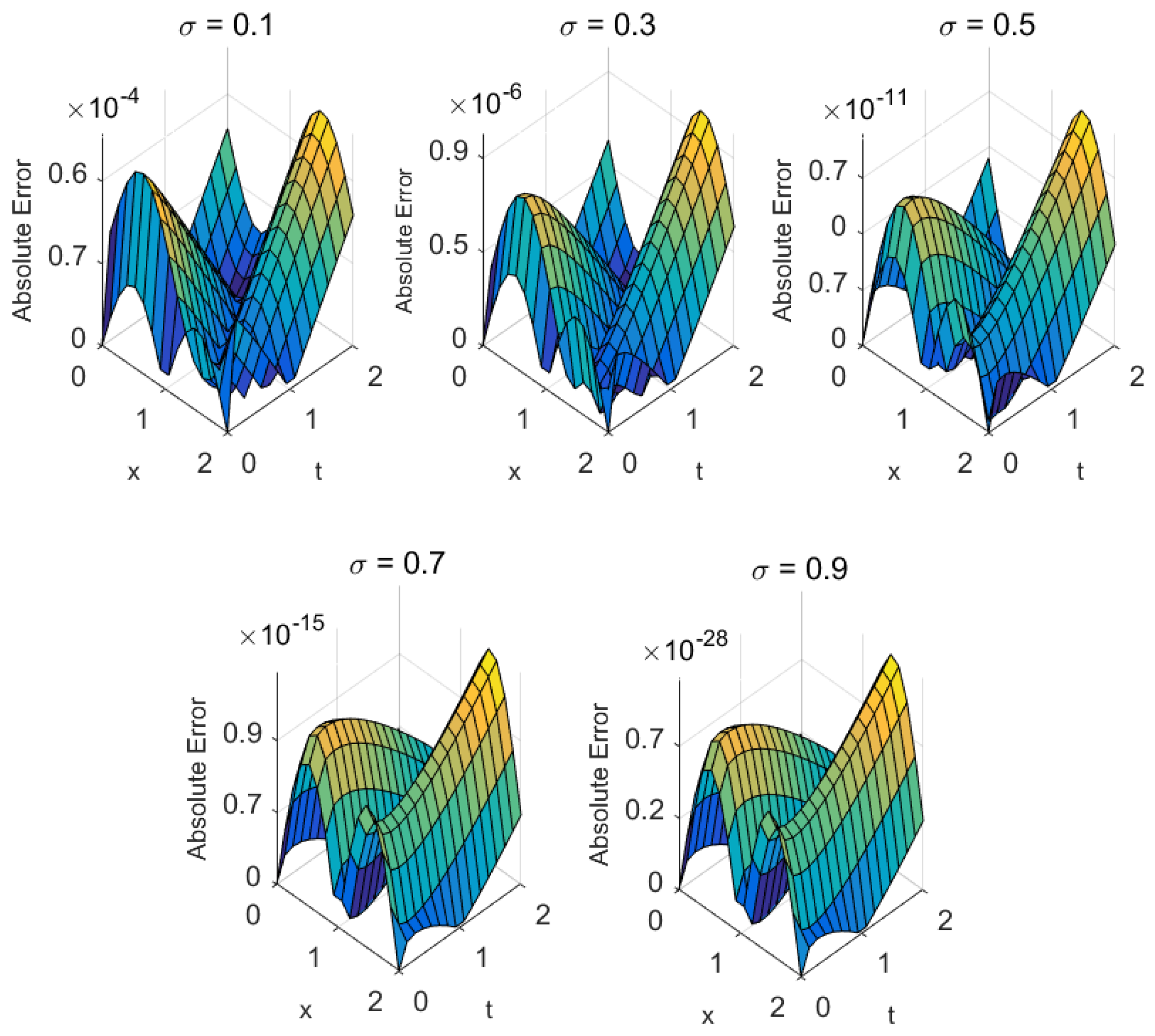
^† All computations were performed using MATLAB VPA with digits = 64, employing a numerical tolerance of ${10}^{-30}$.

summarizes the numerical results obtained with the proposed parallel scheme ${\mathrm{CMM}}_1^{\left[C_3\right]}$ for the considered problem. In these simulations, the initial guess vectors were chosen close to the exact solution (within a tolerance of $0.001$), ensuring efficient convergence while avoiding instabilities that may arise from poor initial approximations. To demonstrate the accuracy and robustness of the scheme across different problem scales and fractional dynamics, the table reports computed solutions for a range of spatial grid sizes and fractional-order parameters $\sigma$. Table 11 also provides a direct comparison between the proposed methodology and established approaches from the literature, offering a comprehensive performance assessment. Based on these results, Figure 6 and Figure 7 illustrate the exact and approximate solutions of (71), together with the corresponding absolute errors. For fractional parameters $\sigma \approx 1$, the comparison was carried out with grid sizes of 120 and 180, enabling evaluation in the near-integer regime. This analysis confirms the efficacy, accuracy, and computational advantages of the ${\mathrm{CMM}}_1^{\left[C_3\right]}$ scheme, validating its suitability for high-precision fractional-order simulations in practical applications.

Table 12. Error comparison between parallel schemes for solving (79) with $\sigma \approx 1$ using Criteria I and II without using the parfor function in MATLAB.

Metric	${\mathrm{WDM}}^{\left[{\mathit{C}}_2\right]}$	${\mathrm{ACM}}^{\left[{\mathit{C}}_2\right]}$	${\mathrm{ELM}}^{\left[{\mathit{C}}_3\right]}$	${\mathrm{CMM}}_1^{\left[{\mathit{C}}_3\right]}$	${\mathrm{CMM}}_2^{\left[{\mathit{C}}_3\right]}$
		Using Criterion I
${\parallel .\parallel }_2$-norm	$1.03\times {10}^{-5}$	$8.39\times {10}^{-9}$	$6.17\times {10}^{-11}$	$6.00\times {10}^{-25 †}$	$5.54\times {10}^{-20 †}$
${\parallel .\parallel }_{\infty }$-norm	$2.05\times {10}^{-6}$	$2.63\times {10}^{-8}$	$8.70\times {10}^{-12}$	$1.47\times {10}^{-22 †}$	$6.01\times {10}^{-27 †}$
		Using Criterion II
${\parallel .\parallel }_2$-norm	$1.53\times {10}^{-6}$	$3.17\times {10}^{-7}$	$1.05\times {10}^{-12}$	$9.30\times {10}^{-19 †}$	$5.04\times {10}^{-23 †}$
${\parallel .\parallel }_{\infty }$-norm	$6.04\times {10}^{-4}$	$3.40\times {10}^{-10}$	$8.50\times {10}^{-11}$	$1.31\times {10}^{-25 †}$	$4.50\times {10}^{-29 †}$

^† All computations were performed using MATLAB variable precision arithmetic (VPA) with digits = 64, employing a numerical tolerance of ${10}^{-30}$.

reports the numerical results obtained with the proposed parallel scheme ${\mathrm{CMM}}_2^{\left[C_3\right]}$ for the problem under consideration. In these simulations, the initial vector estimates were selected within $0.001$ of the exact solution to ensure an efficient iterative process and to avoid instabilities that may arise from inaccurate initial approximations. To demonstrate the stability and reliability of the combined ${\mathrm{CMM}}_1^{\left[C_3\right]}$–${\mathrm{CMM}}_2^{\left[C_3\right]}$ framework across different problem scales and fractional dynamics, the table presents computed solutions for a range of spatial grid points and fractional-order parameters $\sigma$.

Table 13. Overall performance of parallel schemes for solving (79) without MATLAB parfor parallelization.

Metric	Iterations (n)	Max- Error	Percentage Convergence	Basic Ops $[\pm ,\times ,÷]$	Memory Usage (MB)	COC
${\mathrm{WDM}}^{\left[C_2\right]}$	23	$4.55\times {10}^{-5}$	35.09%	47	76.147	2.00
${\mathrm{ACM}}^{\left[C_2\right]}$	21	$5.08\times {10}^{-8}$	41.96%	51	67.347	2.03
${\mathrm{ELM}}^{\left[C_3\right]}$	16	$6.51\times {10}^{-10}$	65.13%	50	53.704	2.01
${\mathrm{CMM}}_1^{\left[C_3\right]}$	11	$7.52\times {10}^{-13}$	77.04%	54	49.500	3.12
${\mathrm{CMM}}_2^{\left[C_3\right]}$	10	$8.55\times {10}^{-15}$	93.98%	36	44.413	3.00

further provides a performance assessment by comparing the proposed strategy against established methods from the literature. In particular, for fractional parameters $\sigma \approx 1$, grid sizes of 120 and 180 were considered, allowing evaluation in the near-integer regime. This comparison highlights the efficiency, accuracy, and computational advantages of the ${\mathrm{CMM}}_1^{\left[C_3\right]}$ scheme, confirming its suitability for high-precision fractional-order simulations in practical applications.

The overall performance of the proposed parallel schemes is summarized in Table 13, for a fractional parameter $\sigma =0.9$ and grid sizes of 120 and 180.

Table 13 clearly demonstrates that, across key performance metrics—including the number of iterations, maximum error, percentage convergence, total arithmetic operations, memory usage, and computational order of convergence (COC)—the proposed method significantly outperforms existing approaches. Random initial guess vectors were employed to analyze the global convergence of parallel techniques for solving (79). This procedure substantially enhanced robustness and efficiency across a wide range of problem instances. The random initial guess vectors used for the bio-heat problem are reported in

Table 14. Discretization details of the bio-heat transfer problem used for generating random initial guess vectors.

Application	Domain $(\mathit{x},\mathit{t})$	Recorded Variables	Approx. Data Size
Bio-heat transfer	$x\in [0,1],t\in [0,1]$	$x_i,t^k,u_{i-1}^{k-1},u_i^{k-1},u_{i+1}^{k-1}$	$\sim M\times N$

and

Table 15. Example of a random initial guess vector drawn from 100 MATLAB-generated test samples.

${\mathit{x}}_{\mathit{i}}$	${\mathit{t}}^{\mathit{k}}$	${\mathit{u}}_{\mathit{i}-1}^{\mathit{k}-1}$	${\mathit{u}}_{\mathit{i}}^{\mathit{k}-1}$	${\mathit{u}}_{\mathit{i}+1}^{\mathit{k}-1}$	${\mathit{u}}_{\mathit{i}}^{\mathit{k}}$
0.03333	0.02000	2.1967	2.1976	2.1984	2.1980
0.73333	0.04000	2.8693	2.8712	2.8730	2.8721
0.46667	0.08000	2.6587	2.6599	2.6610	2.6605
⋮ (remaining entries omitted)

.

The results of the adaptive self-adjustment of initial guess values, as outlined in Algorithm 2, are presented in

Table 16. Maximum error outcomes of parallel schemes ${\mathrm{CMM}}_1^{\left[C_3\right]}$–${\mathrm{CMM}}_2^{\left[C_3\right]}$ implemented via MATLAB parfor for solving (79).

$\mathit{\sigma }$	0.1	0.3	0.5	0.7	0.9	Mem U
		Using Criteria-I
${\mathrm{CMM}}_1^{\left[C_3\right]}$	$2.50\times {10}^{-6}$	$7.55\times {10}^{-7}$	$4.00\times {10}^{-13}$	$7.56\times {10}^{-21 †}$	$4.25\times {10}^{-27 †}$	$67.100$
${\mathrm{CMM}}_2^{\left[C_3\right]}$	$4.50\times {10}^{-6}$	$8.45\times {10}^{-9}$	$9.80\times {10}^{-18}$	$6.54\times {10}^{-25 †}$	$6.55\times {10}^{-30 †}$	$69.537$
		Using Criteria-II
${\mathrm{CMM}}_1^{\left[C_3\right]}$	$2.50\times {10}^{-4}$	$3.56\times {10}^{-6}$	$7.50\times {10}^{-14}$	$3.56\times {10}^{-19 †}$	$7.52\times {10}^{-23 †}$	$58.641$
${\mathrm{CMM}}_2^{\left[C_3\right]}$	$5.52\times {10}^{-5}$	$7.54\times {10}^{-8}$	$3.65\times {10}^{-15}$	$4.65\times {10}^{-23 †}$	$1.14\times {10}^{-26 †}$	$51.112$

^† All computations were performed using MATLAB variable precision arithmetic (VPA) with digits = 64, employing a numerical tolerance of ${10}^{-30}$.

for both Criterion I and Criterion II.

Table 16 presents the accuracy of the proposed scheme in solving CTFPDEs for various parameter values. The results for grid sizes of 120 and 180 clearly demonstrate that the methods achieve higher accuracy than earlier approaches.

Table 17. Consistency analysis using random initial guess vectors for parallel schemes ${\mathrm{CMM}}_1^{\left[C_3\right]}$–${\mathrm{CMM}}_2^{\left[C_3\right]}$ implemented with MATLAB parfor for solving (79).

Metric	Average Iterations	COC	CPU Time (s)	Percentage Convergence	Memory Usage (MB)
Using Criterion I
${\mathrm{CMM}}_1^{\left[C_3\right]}$	17	$2.0905$	$2.3995$	$76.47\%$	$41.14$
${\mathrm{CMM}}_2^{\left[C_3\right]}$	16	$3.0336$	$2.1887$	$97.64\%$	$46.60$
Using Criterion II
${\mathrm{CMM}}_1^{\left[C_3\right]}$	15	$2.0126$	$2.1166$	$91.33\%$	$47.12$
${\mathrm{CMM}}_2^{\left[C_3\right]}$	16	$3.3268$	$2.0066$	$94.57\%$	$46.40$

provides the overall consistency analysis, performed with a random set of initial values. The results in Table 17 confirm that the combined ${\mathrm{CMM}}_1^{\left[C_3\right]}$–${\mathrm{CMM}}_2^{\left[C_3\right]}$ scheme outperforms existing methods (${\mathrm{WDM}}^{\left[C_2\right]}$, ${\mathrm{ACM}}^{\left[C_2\right]}$, ${\mathrm{ELM}}^{\left[C_3\right]}$) in both accuracy and stability. Across all evaluation metrics—including the average number of iterations, computational time (seconds), percentage convergence, and memory usage—the proposed methods consistently surpass competing approaches under both Criterion I and Criterion II.

The results obtained from the MATLAB parfor-based parallel implementation are reported in

Table 18. Outcomes of parallel schemes ${\mathrm{CMM}}_1^{\left[C_3\right]}$–${\mathrm{CMM}}_2^{\left[C_3\right]}$ implemented via MATLAB parfor for solving (79). Errors are reported with a double-precision cap; see footnote for VPA residuals.

Metric	${\mathit{T}}_{\mathbf{seri}}$ (s)	${\mathit{T}}_{\mathbf{para}}$ (s)	${\mathit{\varphi }}_{\mathbf{speed}}$	Maximum Error	Percentage Convergence	Memory Usage (MB)
		Using Criterion I
${\mathrm{CMM}}_1^{\left[C_3\right]}$	$2.34$	$1.67$	$1.40$	$\le 2.22\times {10}^{-16 †}$	$91.47\%$	$25.93$
${\mathrm{CMM}}_2^{\left[C_3\right]}$	$3.91$	$1.05$	$3.73$	$\le 2.22\times {10}^{-16 †}$	$93.17\%$	$20.12$
		Using Criterion II
${\mathrm{CMM}}_1^{\left[C_3\right]}$	$7.61$	$2.45$	$3.11$	$\le 2.22\times {10}^{-16 †}$	$95.57\%$	$19.19$
${\mathrm{CMM}}_2^{\left[C_3\right]}$	$8.81$	$2.81$	$3.13$	$\le 2.22\times {10}^{-16 †}$	$97.78\%$	$17.20$

^† All computations used MATLAB VPA (with digits = 64). Raw VPA residuals for Max-Error were $1.3\times {10}^{-31}$, $4.1\times {10}^{-27}$ (Criterion I) and $1.1\times {10}^{-26}$, $5.1\times {10}^{-23}$ (Criterion II). For consistent reporting across floating-point environments, the displayed Max-Error values are $min\{\mathrm{VPA}\mathrm{residual},2.22\times {10}^{-16}\}$, ensuring comparability with IEEE double precision.

.

All test cases demonstrate substantial acceleration with the proposed MATLAB parfor-based parallelization of the schemes. On a four-core machine, the parallel implementation achieved a speedup ratio of approximately $3.73$–$4\times$, as reported in Table 18, confirming efficient utilization of the available cores. Importantly, both the maximum error and percentage convergence remained unchanged compared to the serial implementation, indicating that accuracy is fully preserved under parallel execution.

Physical Behavior of the Brain Signal Propagation Model. In the brain signal propagation model, the fractional-order derivative incorporates memory effects in neuronal and hemodynamic dynamics, while nonlinear blood flow terms account for feedback between vascular response and signal transmission. These structural properties were reflected in the choice of numerical parameters, such as time step and spatial discretization, which were selected to ensure both accuracy and computational efficiency.

• Step size and tolerance were chosen to balance accuracy and convergence in the presence of fractional dynamics and nonlinear flow effects.
• Numerical results showed that the proposed parallel scheme accurately reproduced signal propagation patterns while preserving key physiological features.
• Fractional order, nonlinear blood flow, and discretization parameters jointly influenced computational cost and convergence rate.

3.2.3. Fractional Heart Tissue Electrical Conduction with Nonlinear Reaction [53]

The fractional heart tissue electrical conduction model with nonlinear response provides a refined mathematical framework for describing the propagation of electrical signals in cardiac tissue, incorporating memory effects and complex cell interactions through fractional calculus. Unlike classical integer-order models, this approach employs fractional derivatives—typically in the Caputo or Riemann–Liouville form—to capture anomalous diffusion and hereditary properties that reflect the heterogeneity and microstructural complexity of heart tissue.

This framework is particularly valuable for modeling the dynamics of gap junctions and ion channels, where nonlinear reaction terms reproduce the biochemical processes and voltage-dependent ionic currents responsible for generating and propagating action potentials. By coupling fractional reaction–diffusion equations with nonlinear source terms, the model effectively replicates realistic processes such as wavefront slowing, reentry phenomena, and the complex spatiotemporal patterns characteristic of cardiac arrhythmia. The fractional-order parameter serves as a tuning mechanism, interpolating between normal diffusion and sub-diffusion, thereby enabling a more accurate representation of delayed conduction and memory-dependent effects typical of diseased or fibrotic myocardium.

This enhanced modeling capability not only deepens the understanding of pathological conduction but also provides a powerful tool for designing targeted therapeutic strategies, including electrical pacing and ablation therapy in clinical electrophysiology.

In a one-dimensional tissue segment $x\in [0,2]$, the spatiotemporal evolution of the fractional cardiac tissue electrical conduction with nonlinear reaction $u(x,t)$ is modeled by a time-fractional reaction–diffusion equation [54]:

$$\left\{\begin{array}{cc}{\displaystyle \frac{{\partial }^{\sigma }u}{\partial t^{\sigma }}=\frac{{\partial }^{2}u}{\partial x^2}+\frac{\partial u}{\partial x}+u(x,t)+u^3(x,t)+f(x,t),}\hfill & x\in [0,2],t\in [0,2],\hfill \\ u(x,0)=0,\hfill \\ u(0,t)=t^{\sigma },u(2,t)=0.\hfill \end{array}\right.$$

(80)

where the source term $f(x,t)$ is chosen so that the exact solution

$$u(x,t)=\left(1-{\displaystyle \frac{x}{2}}\right)t^{\sigma }$$

(81)

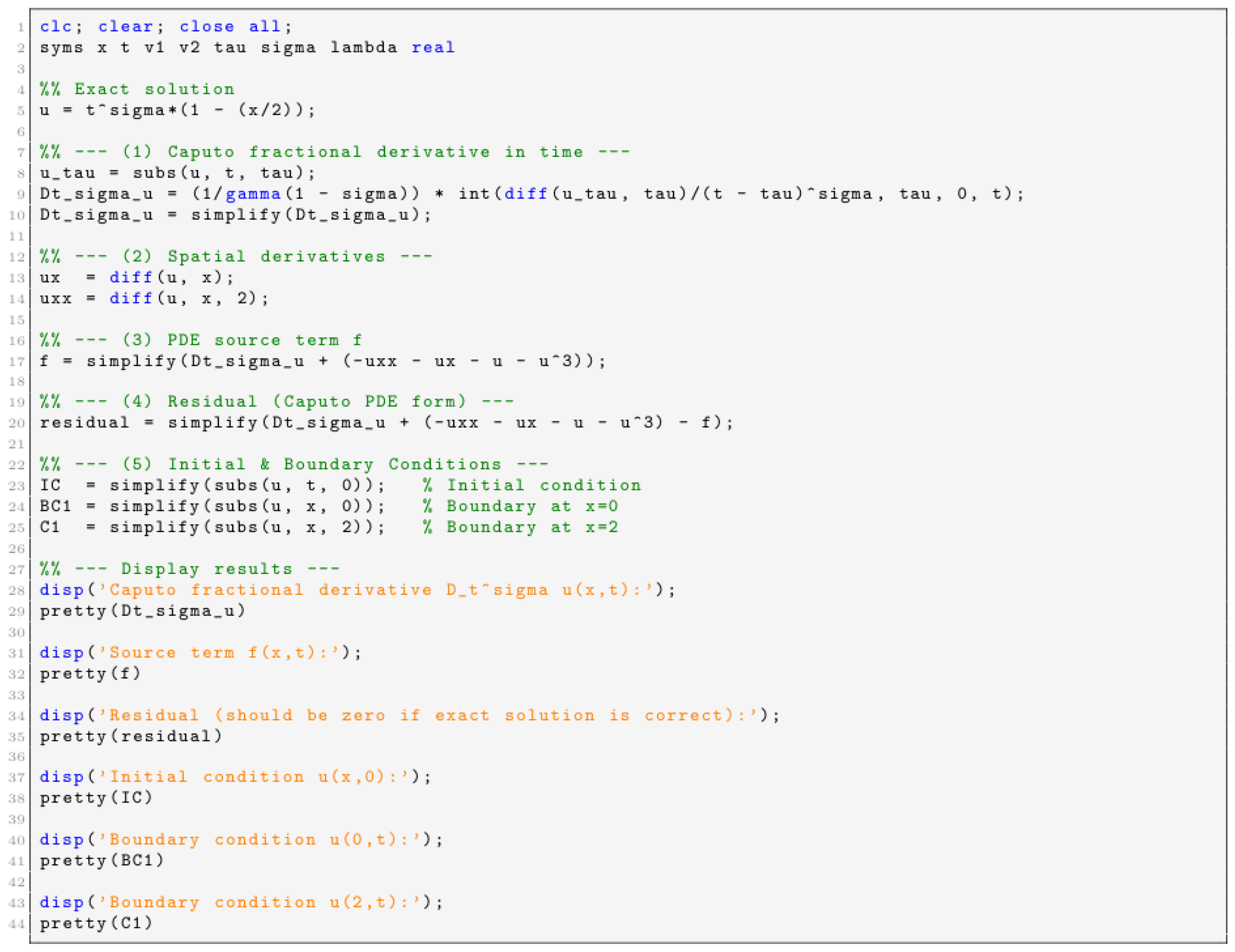
satisfies the PDE exactly (see MATLAB symbolic script in Appendix A.3, Figure A3). In particular, the source term is defined as

$$f(x,t)={\displaystyle \frac{1}{8}}\left({(-2+x)}^3{t}^{3\sigma }+4t^{\sigma }(-1+x)\right)+{\displaystyle \frac{4x-8}{8}}{Q}_2^{[\ast ]},$$

(82)

where

$$Q_2^{[\ast ]}={\Gamma }^{-1}(-\sigma ){\int }_0^t{\tau }^{\sigma -2}{(t-\tau )}^{-\sigma }d\tau .$$

(83)

Problem characterization:

• Spatial domain: $x\in [0,2]$, discretized into N intervals with spacing $h=L/N$.
• Time domain: $t\in [0,2]$, discretized into M intervals with spacing $\tau =T/M$.
• Grid nodes: $x_i=ih$, $i=0,\dots ,N$; $t_n=n\tau$, $n=0,\dots ,M$.
• Unknowns: $u_i^n\approx u(x_i,t_n)$.

By applying approximations (66)–(68) to (80), the following nonlinear system of equations is obtained:

$${\displaystyle \frac{1}{\tau \Gamma (2-\sigma )}}{\displaystyle \sum _{k=1}^{n-1}}{w}_k^{\left(n\right)}{u}_i^k={\displaystyle \frac{u_{i+1}^n-2u_i^n+u_{i-1}^n}{h^2}}+{\displaystyle \frac{u_{i+1}^n-u_{i-1}^n}{2h}}+u_i^n+{\left(u_i^n\right)}^3+f_i^n,$$

(84)

where

$$f_i^n=f(x_i,t^n)={\displaystyle \frac{\Gamma (1+\sigma )}{1+x_i^2}}-{\left(t^n\right)}^{\sigma }\left({\displaystyle \frac{6x_i^2-2}{{(1+x_i^2)}^3}}-{\displaystyle \frac{2x_i}{{(1+x_i^2)}^2}}+{\displaystyle \frac{1}{1+x_i^2}}\right).$$

(85)

The system can be written in matrix form as

$${\displaystyle \frac{1}{\tau \Gamma (2-\sigma )}}{\displaystyle \sum _{k=1}^{n-1}}{w}_k^{\left(n\right)}{\mathbf{u}}^k={\mathbf{D}}_1{\mathbf{u}}^n+{\mathbf{D}}_2{\mathbf{u}}^n+{\mathbf{u}}^n+{\left({\mathbf{u}}^n\right)}^3+{\mathbf{f}}^n,$$

(86)

where

• ⊙ denotes element-wise operations;
• ${\mathbf{f}}^n={[f_1^n,f_2^n,\dots ,f_{N-1}^n]}^T,$

and the matrices ${\mathbf{D}}_1$ and ${\mathbf{D}}_2$ are defined in (72)–(73).

The numerical results obtained with the proposed parallel scheme ${\mathrm{CMM}}_1^{\left[C_3\right]}$ are summarized in

Table 19. Maximum error norms of parallel scheme ${\mathrm{CMM}}_2^{\left[C_3\right]}$ without MATLAB parfor for different $\sigma$ values.

Grid Points	${\parallel .\parallel }_2$-Norm	${\parallel .\parallel }_{\mathit{\infty }}$-Norm	CPU Time (s)
	$\sigma =0.1$
$30,50$	$9.030\times {10}^{-4}$	$1.117\times {10}^{-3}$	$0.049$
$60,90$	$1.051\times {10}^{-4}$	$9.853\times {10}^{-4}$	$0.124$
$120,180$	$7.790\times {10}^{-4}$	$5.201\times {10}^{-3}$	$0.258$
	$\sigma =0.3$
$30,50$	$1.901\times {10}^{-8}$	$9.376\times {10}^{-9}$	$0.065$
$60,90$	$5.587\times {10}^{-9}$	$7.807\times {10}^{-7}$	$0.129$
$120,180$	$1.007\times {10}^{-8}$	$7.056\times {10}^{-8}$	$0.208$
	$\sigma =0.5$
$30,50$	$6.155\times {10}^{-15}$	$1.110\times {10}^{-14}$	$0.071$
$60,90$	$5.009\times {10}^{-12}$	$5.004\times {10}^{-11}$	$0.135$
$120,180$	$6.509\times {10}^{-15}$	$9.008\times {10}^{-14}$	$0.286$
	$\sigma =0.7$
$30,50$	$1.117\times {10}^{-19 †}$	$1.727\times {10}^{-21 †}$	$0.081$
$60,90$	$1.009\times {10}^{-17 †}$	$3.345\times {10}^{-20 †}$	$0.142$
$120,180$	$5.450\times {10}^{-19 †}$	$2.010\times {10}^{-19 †}$	$0.299$
	$\sigma =0.9$
$30,50$	$3.337\times {10}^{-30 †}$	$7.598\times {10}^{-29 †}$	$0.087$
$60,90$	$7.060\times {10}^{-29 †}$	$8.760\times {10}^{-28 †}$	$0.237$
$120,180$	$7.150\times {10}^{-27 †}$	$4.840\times {10}^{-25 †}$	$0.358$

^† All computations were performed using MATLAB VPA with digits = 64, employing a numerical tolerance of ${10}^{-30}$.

. In these simulations, the initial guess vectors were selected within a tolerance of $0.001$ from the exact solution to ensure efficient convergence and to avoid instabilities due to poor initialization. The table reports computed solutions for a range of spatial grid points and fractional-order parameters $\sigma$, illustrating the robustness and accuracy of the scheme across varying problem scales and fractional dynamics.

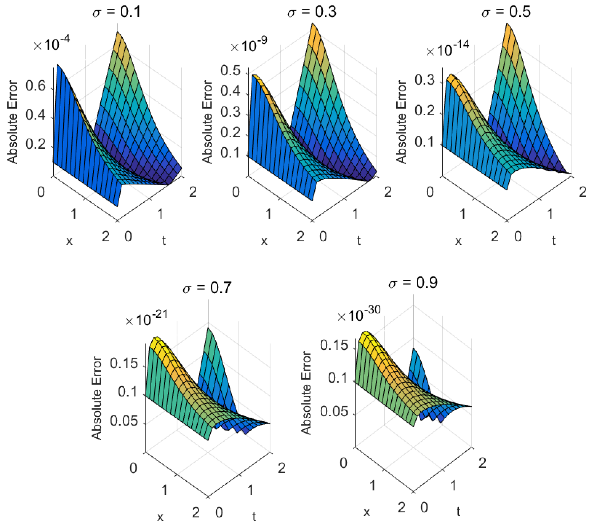
To assess performance, Table 19 also provides a direct comparison with well-established methods from the literature. Based on these results, Figure 8 and Figure 9 present the exact and approximate solutions of (86), together with the corresponding absolute errors, for selected grid sizes 120 and 180 with fractional parameter $\sigma \approx 1$. This near-integer regime highlights the efficiency, accuracy, and computational advantages of the ${\mathrm{CMM}}_1^{\left[C_3\right]}$ scheme, confirming its suitability for high-precision fractional-order simulations in practical applications.

Table 20. Error comparison of parallel schemes for solving (86) with $\sigma \approx 1$, using Criterion I and Criterion II without MATLAB parfor.

Metric	${\mathrm{WDM}}^{\left[{\mathit{C}}_2\right]}$	${\mathrm{ACM}}^{\left[{\mathit{C}}_2\right]}$	${\mathrm{ELM}}^{\left[{\mathit{C}}_3\right]}$	${\mathrm{CMM}}_1^{\left[{\mathit{C}}_3\right]}$	${\mathrm{CMM}}_2^{\left[{\mathit{C}}_3\right]}$
		Using Criterion I
${\parallel .\parallel }_2$-norm	$1.05\times {10}^{-5}$	$9.16\times {10}^{-8}$	$5.43\times {10}^{-11}$	$5.76\times {10}^{-23 †}$	$6.37\times {10}^{-29 †}$
${\parallel .\parallel }_{\infty }$-norm	$7.11\times {10}^{-4}$	$2.98\times {10}^{-6}$	$9.75\times {10}^{-11}$	$4.87\times {10}^{-19 †}$	$1.07\times {10}^{-27 †}$
		Using Criterion II
${\parallel .\parallel }_2$-norm	$3.53\times {10}^{-4}$	$1.41\times {10}^{-7}$	$9.39\times {10}^{-14}$	$2.30\times {10}^{-23 †}$	$1.04\times {10}^{-26 †}$
${\parallel .\parallel }_{\infty }$-norm	$1.14\times {10}^{-6}$	$7.07\times {10}^{-13}$	$4.00\times {10}^{-26}$	$1.40\times {10}^{-28 †}$	$3.45\times {10}^{-21 †}$

^† All computations were performed using MATLAB variable precision arithmetic (VPA) with digits = 64, employing a numerical tolerance of ${10}^{-30}$.

reports the numerical results obtained with the proposed parallel schemes ${\mathrm{CMM}}_1^{\left[C_3\right]}$–${\mathrm{CMM}}_2^{\left[C_3\right]}$ for the problem under consideration. In these simulations, the initial guess vectors were selected within a tolerance of $0.001$ from the exact solution to ensure efficient convergence and to avoid instabilities that may arise from poor initial approximations. The table presents computed solutions for different spatial grid points and fractional-order parameters $\sigma$, demonstrating the stability and accuracy of the scheme across varying problem scales and fractional dynamics.

For a meaningful performance assessment,

Table 21. Overall performance of parallel schemes for solving (86) without MATLAB parfor parallelization.

Metric	Iterations (n)	Max- Error	Percentage Convergence	Basic Ops $[\pm ,\times ,÷]$	Memory Usage (MB)	COC
${\mathrm{WDM}}^{\left[C_2\right]}$	23	$7.65\times {10}^{-7}$	35.05%	47	91.147	2.00
${\mathrm{ACM}}^{\left[C_2\right]}$	17	$6.50\times {10}^{-7}$	39.56%	51	86.000	1.99
${\mathrm{ELM}}^{\left[C_3\right]}$	16	$5.24\times {10}^{-9}$	57.74%	50	68.764	1.86
${\mathrm{CMM}}_1^{\left[C_3\right]}$	15	$3.64\times {10}^{-10}$	76.55%	54	64.007	3.01
${\mathrm{CMM}}_2^{\left[C_3\right]}$	9	$5.70\times {10}^{-14}$	93.86%	36	59.453	3.11

provides a direct comparison with established methods from the literature, namely, ${\mathrm{WDM}}^{\left[C_2\right]}$, ${\mathrm{ACM}}^{\left[C_2\right]}$, and ${\mathrm{ELM}}^{\left[C_3\right]}$. This comparison, conducted for grid sizes 120 and 180 with fractional parameter $\sigma \approx 1$, highlights the superior efficiency, precision, and computational advantages of the proposed ${\mathrm{CMM}}_1^{\left[C_3\right]}$–${\mathrm{CMM}}_2^{\left[C_3\right]}$ schemes, confirming their suitability for high-accuracy fractional-order simulations in practical applications.

The overall performance of the parallel schemes is summarized in Table 21, considering a fractional parameter $\sigma =0.9$ and grid sizes of 120 and 180.

Table 21 demonstrates that, across key performance metrics—including the number of iterations, maximum error, percentage convergence, total arithmetic operations, memory usage, and computational order of convergence (COC)—the proposed method significantly outperforms existing approaches. To analyze the global convergence of the parallel techniques for solving (86), random initial guess vectors were employed. This procedure substantially improves robustness and efficiency across a wide range of problem instances. The random initial guess vectors used for the bio-heat problem are reported in

Table 22. Discretization details of the bio-heat transfer problem used for generating random initial guess vectors.

Application	Domain $(\mathit{x},\mathit{t})$	Recorded Variables	Data Size (Approx.)
Bio-heat transfer	$x\in [0,1],t\in [0,1]$	$x_i,t^k,u_{i-1}^{k-1},u_i^{k-1},u_{i+1}^{k-1}$	$\sim M\times N$

and

Table 23. Example of a random initial guess vector drawn from 100 MATLAB-generated test samples.

${\mathit{x}}_{\mathit{i}}$	${\mathit{t}}^{\mathit{k}}$	${\mathit{u}}_{\mathit{i}-1}^{\mathit{k}-1}$	${\mathit{u}}_{\mathit{i}}^{\mathit{k}-1}$	${\mathit{u}}_{\mathit{i}+1}^{\mathit{k}-1}$	${\mathit{u}}_{\mathit{i}}^{\mathit{k}}$
0.03333	0.02000	0.00000	0.00000	0.00000	0.01967
0.73333	0.04000	0.00000	0.01967	0.00000	0.02533
0.46667	0.08000	0.02533	0.00000	0.00000	0.06133
⋮ (remaining entries omitted)

.

The outcomes of the adaptive self-adjustment of the initial guess values, as described in Algorithm 2, are reported in

Table 24. Maximum error outcomes of parallel schemes ${\mathrm{CMM}}_1^{\left[C_3\right]}$–${\mathrm{CMM}}_2^{\left[C_3\right]}$ implemented via MATLAB parfor for solving (86).

$\mathit{\sigma }$	0.1	0.3	0.5	0.7	0.9	Mem U
		Using Criterion I
${\mathrm{CMM}}_1^{\left[C_3\right]}$	$8.70\times {10}^{-4}$	$7.13\times {10}^{-8}$	$6.87\times {10}^{-11}$	$3.47\times {10}^{-23}$	$8.11\times {10}^{-27}$	$71.906$
${\mathrm{CMM}}_2^{\left[C_3\right]}$	$7.64\times {10}^{-5}$	$9.51\times {10}^{-9}$	$3.34\times {10}^{-15}$	$2.21\times {10}^{-19}$	$7.00\times {10}^{-25}$	$56.617$
		Using Criterion II
${\mathrm{CMM}}_1^{\left[C_3\right]}$	$4.53\times {10}^{-3}$	$4.32\times {10}^{-6}$	$1.80\times {10}^{-12}$	$7.98\times {10}^{-23 †}$	$2.70\times {10}^{-26 †}$	$66.755$
${\mathrm{CMM}}_2^{\left[C_3\right]}$	$3.05\times {10}^{-5}$	$1.72\times {10}^{-7}$	$5.77\times {10}^{-14}$	$3.60\times {10}^{-26 †}$	$3.41\times {10}^{-29 †}$	$51.975$

^† All computations were performed using MATLAB variable precision arithmetic (VPA) with digits = 64, employing a numerical tolerance of ${10}^{-30}$.

for both Criterion I and Criterion II.

The accuracy of the proposed approaches, ${\mathrm{CMM}}_1^{\left[C_3\right]}$–${\mathrm{CMM}}_2^{\left[C_3\right]}$, in solving CTFPDEs for various parameter values is reported in Table 24. For grid sizes of 120 and 180, the methods achieve higher accuracy than previously established approaches.

Table 25. Consistency analysis using random initial guess vectors in parallel schemes ${\mathrm{CMM}}_1^{\left[C_3\right]}$–${\mathrm{CMM}}_2^{\left[C_3\right]}$ implemented in MATLAB parfor for solving (86).

Method	Average Iterations	COC	CPU Time (s)	Percentage Convergence	Memory Usage (MB)
Using Criterion I
${\mathrm{CMM}}_1^{\left[C_3\right]}$	23	$2.0995$	$2.3005$	$74.74\%$	$87.20$
${\mathrm{CMM}}_2^{\left[C_3\right]}$	19	$3.0746$	$2.8745$	$97.91\%$	$76.60$
Using Criterion II
${\mathrm{CMM}}_1^{\left[C_3\right]}$	14	$2.1187$	$2.6146$	$87.06\%$	$81.12$
${\mathrm{CMM}}_2^{\left[C_3\right]}$	8	$3.0199$	$2.6006$	$93.33\%$	$64.40$

presents the overall consistency analysis, performed with a random set of initial values. The results clearly indicate that ${\mathrm{CMM}}_1^{\left[C_3\right]}$–${\mathrm{CMM}}_2^{\left[C_3\right]}$ outperform existing methods (${\mathrm{WDM}}^{\left[C_2\right]}$, ${\mathrm{ACM}}^{\left[C_2\right]}$, ${\mathrm{ELM}}^{\left[C_3\right]}$) in both accuracy and stability. Under both Criterion I and Criterion II, the schemes consistently deliver superior performance across all evaluation metrics, including the average number of iterations, computational time (seconds), percentage convergence, and memory usage.

The results obtained from the MATLAB parfor-based parallelization of the proposed schemes are presented in

Table 26. Outcomes of parallel schemes ${\mathrm{CMM}}_1^{\left[C_3\right]}$–${\mathrm{CMM}}_2^{\left[C_3\right]}$ implemented via MATLAB parfor for solving (86). Errors are reported with a double-precision cap; see footnote for VPA residuals.

Metric	${\mathit{T}}_{\mathbf{seri}}$ (s)	${\mathit{T}}_{\mathbf{para}}$ (s)	${\mathit{\varphi }}_{\mathbf{speed}}$	Maximum Error	Percentage Convergence	Memory Usage (MB)
		Using Criterion I
${\mathrm{CMM}}_1^{\left[C_3\right]}$	$3.87$	$1.99$	$1.94$	$\le 2.22\times {10}^{-16 †}$	$80.14\%$	$45.13$
${\mathrm{CMM}}_2^{\left[C_3\right]}$	$4.90$	$1.37$	$3.59$	$\le 2.22\times {10}^{-16 †}$	$83.55\%$	$39.23$
		Using Criterion II
${\mathrm{CMM}}_1^{\left[C_3\right]}$	$7.59$	$3.15$	$2.41$	$\le 2.22\times {10}^{-16 †}$	$89.34\%$	$31.88$
${\mathrm{CMM}}_2^{\left[C_3\right]}$	$8.15$	$2.17$	$3.76$	$\le 2.22\times {10}^{-16 †}$	$93.01\%$	$29.69$

^† All computations used MATLAB VPA (with digits = 64). Raw VPA residuals for Max-Error were $8.3\times {10}^{-27}$, $2.0\times {10}^{-29}$ (Criterion I) and $6.0\times {10}^{-28}$, $1.9\times {10}^{-25}$ (Criterion II). For consistent reporting across floating-point environments, the displayed Max-Error values are $min\{\mathrm{VPA}\mathrm{residual},2.22\times {10}^{-16}\}$, ensuring comparability with IEEE double precision.

.

Physical Behavior of the Heart Tissue Electrical Conduction Model: In the fractional heart tissue model, the fractional-order time derivative captures memory effects in electrical conduction, while the nonlinear reaction term characterizes ionic current dynamics and cardiac cell excitability. To enable accurate and efficient simulation of cardiac electrical activity, numerical parameters such as the time step and spatial discretization were carefully selected in accordance with these structural properties.

• Step size and tolerance were adjusted to balance precision and convergence in the presence of fractional dynamics and nonlinear ionic interactions.
• Numerical results confirmed that the proposed approach accurately reproduced the spatiotemporal propagation of electrical signals in cardiac tissue.

3.3. Comparative Discussion of Biomedical Examples

To evaluate the performance of the proposed parallel approaches, we conducted a comparative study across the three biomedical models, using both deterministic closed-form initial guesses and random initial vectors, together with MATLAB’s parfor implementation. Table 2, Table 17 and Table 25 provide a summary of the main findings.

First, Table 3, Table 4 and Table 5, Table 11, Table 12 and Table 13 and Table 19, Table 20 and Table 21 show that the proposed ${\mathrm{CMM}}_2^{\left[C_3\right]}$ scheme consistently achieves lower error norms than existing iterative approaches for fixed fractional orders $\sigma$. In particular, when $\sigma \approx 1$, the method yields a notable reduction in residual error, confirming its stability in the classical limit. Moreover, the results in Table 4 indicate that the proposed methods are both faster and more accurate than earlier schemes, even without parallelization.

Second, Table 17 and Table 25 examine the effect of random initial vectors. The results demonstrate that the proposed strategies maintain robust convergence and consistency across trials, even with randomly generated initializations, highlighting improved algorithmic stability.

Finally, Table 9, Table 10, Table 16, Table 18, Table 24 and Table 26 assess the influence of MATLAB’s parfor-based parallelization. Although parfor differs from OpenMP in memory management, the implementation significantly reduces CPU time, particularly for problems with dense fractional memory terms. Importantly, accuracy is fully preserved under parallel execution, and the observed speedup confirms the scalability of the proposed methods to multi-core architectures.

Overall, the comparative results across the biomedical examples reveal several key trends:

• Mathematical structure: Biomedical models with higher-order nonlinearities or significant fractional memory effects (e.g., cardiac conduction) tend to exhibit slower convergence. Nonetheless, the proposed methods ensure steady residual decay and maintain accuracy even under stiff nonlinear dynamics (see Figure 4, Figure 5, Figure 6, Figure 7, Figure 8 and Figure 9).
• Numerical parameters: Smaller step sizes and high-precision VPA computations reduce local truncation error and further improve accuracy. In addition, adaptive random initialization yields consistent results across all three biomedical applications.
• Efficiency: The proposed parallel schemes, particularly ${\mathrm{CMM}}_2^{\left[C_3\right]}$, reliably reduce CPU time and maximum error compared to classical fractional iterative methods. Performance gains become increasingly pronounced for larger problem sizes and denser fractional memory terms.
• Stability under perturbations: Convergence is preserved even when random initial vectors, parameter fluctuations, or noise in boundary conditions are introduced. This resilience is especially important for biomedical applications, where data uncertainty is inherent.
• Parallel scalability: Although MATLAB’s parfor differs from OpenMP in memory distribution, the results confirm effective parallel speedup on multi-core architectures. The scalability of the proposed approach makes it suitable for high-dimensional and long-time fractional simulations.
• Computational cost: The hierarchical formulation of the parallel schemes controls memory usage, delivering a favorable cost-to-accuracy ratio. Even for nonlinear biological PDEs with strong fractional effects, the proposed methods remain computationally competitive.
• Biomedical relevance: Each biomedical application represents a distinct physiological process—drug transport, neuronal dynamics, and cardiac tissue excitation. In all cases, the proposed methods produced reliable results, underscoring their translational potential in real-world biomedical modeling.

This comparative analysis demonstrates that the proposed approaches not only enhance accuracy and efficiency but also provide a reliable foundation for solving a broad class of biomedical fractional models, thereby extending their practical applicability beyond existing methods.

4. Conclusions

In this paper, two parallel techniques for solving CTFPDEs were developed and analyzed. Theoretical results established second- and third-order convergence, while the implementation exploited diagonal and element-wise multiplications of the Weierstrass correction to efficiently approximate the solutions. Several benchmark problems from biomedical engineering were employed to evaluate the accuracy, stability, and consistency of the proposed schemes.

The numerical results, summarized in Table 1, Table 2, Table 3, Table 4, Table 5, Table 6, Table 7, Table 8, Table 9, Table 10, Table 11, Table 12, Table 13, Table 14, Table 15, Table 16, Table 17, Table 18, Table 19, Table 20, Table 21, Table 22, Table 23, Table 24, Table 25 and Table 26 and Figure 1, Figure 2, Figure 3, Figure 4, Figure 5, Figure 6, Figure 7, Figure 8 and Figure 9, demonstrate that the new methods consistently outperform existing approaches in terms of residual errors (in both ${\ell }_2$- and ${\ell }_{\infty }$-norms), memory efficiency, computational time, and percentage convergence. The use of random initial test vectors combined with an adaptive optimization step further enhanced robustness by automatically selecting effective starting points and accelerating convergence. In addition, fractal-based dynamical analysis (Table 2 and Figure 2) confirmed the stability and reliability of the schemes across diverse problem scales.

• Limitations. The present study has some limitations:
  • Parallelization was implemented using MATLAB’s parfor construct rather than low-level OpenMP or GPU-based solutions, which may limit scalability for large-scale problems.
  • Higher-dimensional cases may require additional stability and memory considerations; the numerical studies presented here were restricted to two-dimensional biological PDEs.
  • Exact solutions were constructed for validation, whereas real biomedical data typically contain noise and parameter uncertainty, which were not considered in this work.
• Future work. Several directions are envisioned for extending this study:
  • Implementing the techniques in hybrid CPU–GPU environments to improve scalability and computational speed.
  • Extending the framework to multidimensional biomedical models, such as three-dimensional heart wave propagation.
  • Incorporating uncertainty quantification to account for variability and noise in physiological data.
  • Exploring adaptive step-size control and machine learning-assisted initialization to further improve reliability and convergence.

In summary, the proposed parallel techniques provide a theoretically sound and computationally efficient framework for solving fractional-order PDEs in biomedical engineering. By combining rigorous convergence guarantees with practical efficiency, they offer a powerful tool for modeling complex physiological processes with memory effects, thereby extending the applicability of fractional models in biomedical research and clinical simulation.

References

1. Rathore, A.S.; Mishra, S.; Nikita, S.; Priyanka, P. Bioprocess control: Current progress and future perspectives. Life 2021, 11, 557. [Google Scholar] [CrossRef]
2. Su, W.H.; Chou, C.S.; Xiu, D. Deep learning of biological models from data: Applications to ODE models. Bull. Math. Biol. 2021, 83, 19. [Google Scholar] [CrossRef]
3. Cruz, D.A.; Kemp, M.L. Hybrid computational modeling methods for systems biology. Prog. Biomed. Eng. 2021, 4, 012002. [Google Scholar] [CrossRef]
4. Enderle, J.D.; Ropella, K.M.; Kelsa, D.M.; Hallowell, B. Ensuring that biomedical engineers are ready for the real world. IEEE Eng. Med. Biol. Mag. 2002, 21, 59–66. [Google Scholar] [CrossRef] [PubMed]
5. Gu, X.M.; Wu, S.L. A parallel-in-time iterative algorithm for Volterra partial integro-differential problems with weakly singular kernel. J. Comput. Phys. 2020, 417, 109576. [Google Scholar] [CrossRef]
6. Wen, J.; Tian, Y.E.; Skampardoni, I.; Yang, Z.; Cui, Y.; Anagnostakis, F.; Mamourian, E.; Zhao, B.; Toga, A.W.; Zalesky, A.; et al. The genetic architecture of biological age in nine human organ systems. Nat. Aging 2024, 4, 1290–1307. [Google Scholar] [CrossRef]
7. Ghezal, A.; Al Ghafli, A.A.; Al Salman, H.J. Anomalous Drug Transport in Biological Tissues: A Caputo Fractional Approach with Non-Classical Boundary Modeling. Fractal Fract. 2025, 9, 508. [Google Scholar] [CrossRef]
8. Sachse, F.B.; Moreno, A.P.; Seemann, G.; Abildskov, J.A. A model of electrical conduction in cardiac tissue including fibroblasts. Ann. Biomed. Eng. 2009, 37, 874–889. [Google Scholar] [CrossRef]
9. Dai, X.; Wu, D.; Xu, K.; Ming, P.; Cao, S.; Yu, L. Viscoelastic Mechanics: From Pathology and Cell Fate to Tissue Regeneration Biomaterial Development. Acs Appl. Mater. Interfaces 2025, 17, 8751–8770. [Google Scholar] [CrossRef]
10. Peng, C.; Guo, T.; Xie, C.; Bai, X.; Zhou, J.; Zhao, X.; He, E.; Xia, F. mBGT: Encoding brain signals with multimodal brain graph transformer. IEEE Trans. Consum. Electron. 2024, 71, 5812–5823. [Google Scholar] [CrossRef]
11. Kaltenbacher, B.; Rundell, W. Inverse Problems for Fractional Partial Differential Equations; American Mathematical Society: Providence, RI, USA, 2023; Volume 230. [Google Scholar]
12. Mubaraki, A.M.; Nuruddeen, R.I.; Gomez-Aguilar, J.F. Closed-form asymptotic solution for the transport of chlorine concentration in composite pipes. Phys. Scr. 2024, 99, 075201. [Google Scholar] [CrossRef]
13. Lin, C.H.; Liu, C.H.; Chien, L.S.; Chang, S.C. Accelerating pattern matching using a novel parallel algorithm on GPUs. IEEE Trans. Comput. 2012, 62, 1906–1916. [Google Scholar] [CrossRef]
14. Zhao, Y.L.; Gu, X.M.; Ostermann, A. A preconditioning technique for an all-at-once system from Volterra subdiffusion equations with graded time steps. J. Sci. Comput. 2021, 88, 11. [Google Scholar] [CrossRef]
15. He, J.H.; Anjum, N.; He, C.H.; Alsolami, A.A. Beyond laplace and fourier transforms: Challenges and future prospects. Therm. Sci. 2023, 27 Pt B, 5075–5089. [Google Scholar] [CrossRef]
16. Haubold, H.J.; Mathai, A.M.; Saxena, R.K. Mittag-Leffler functions and their applications. J. Appl. Math. 2011, 2011, 298628. [Google Scholar] [CrossRef]
17. Duffy, D.G. Green’s Functions with Applications; Chapman and Hall/CRC: Boca Raton, FL, USA, 2015. [Google Scholar]
18. Hedin, L. New method for calculating the one-particle Green’s function with application to the electron-gas problem. Phys. Rev. 1965, 139, A796. [Google Scholar] [CrossRef]
19. Rainer, B.; Kaltenbacher, B. Existence, uniqueness, and numerical solutions of the nonlinear periodic Westervelt equation. ESAIM Math. Model. Numer. Anal. 2025, 59, 2279–2304. [Google Scholar] [CrossRef]
20. Kumar, M.; Umesh. Recent development of Adomian decomposition method for ordinary and partial differential equations. Int. J. Appl. Comput. Math. 2022, 8, 81. [Google Scholar] [CrossRef]
21. Nadeem, M.; He, J.H.; Islam, A. The homotopy perturbation method for fractional differential equations: Part 1 Mohand transform. Int. J. Numer. Methods Heat Fluid Flow 2021, 31, 3490–3504. [Google Scholar] [CrossRef]
22. Shihab, M.A.; Taha, W.M.; Hameed, R.A.; Jameel, A.; Ibrahim, S.M. Implementation of variational iteration method for various types of linear and nonlinear partial differential equations. Int. J. Electr. Comput. Eng. 2023, 13, 2131–2141. [Google Scholar] [CrossRef]
23. Kamil Jassim, H.; Vahidi, J. A new technique of reduce differential transform method to solve local fractional PDEs in mathematical physics. Int. J. Nonlinear Anal. Appl. 2021, 12, 37–44. [Google Scholar]
24. Li, C.; Zeng, F. Finite difference methods for fractional differential equations. Int. J. Bifurc. Chaos 2012, 22, 1230014. [Google Scholar] [CrossRef]
25. Sacchetti, A.; Bachmann, B.; Löffel, K.; Künzi, U.M.; Paoli, B. Neural networks to solve partial differential equations: A comparison with finite elements. IEEE Access 2022, 10, 32271–32279. [Google Scholar] [CrossRef]
26. Sheng, C.; Cao, D.; Shen, J. Efficient spectral methods for PDEs with spectral fractional Laplacian. J. Sci. Comput. 2021, 88, 4. [Google Scholar] [CrossRef]
27. Rieder, A. A p-version of convolution quadrature in wave propagation. SIAM J. Numer. Anal. 2025, 63, 1729–1756. [Google Scholar] [CrossRef]
28. Figueroa, A.; Jackiewicz, Z.; Löhner, R. Explicit two-step Runge-Kutta methods for computational fluid dynamics solvers. Int. J. Numer. Methods Fluids 2021, 93, 429–444. [Google Scholar] [CrossRef]
29. Salem, M.G.; Abouelregal, A.E.; Elzayady, M.E.; Sedighi, H.M. Biomechanical response of skin tissue under ramp-type heating by incorporating a modified bioheat transfer model and the Atangana–Baleanu fractional operator. Acta Mech. 2024, 235, 5041–5060. [Google Scholar] [CrossRef]
30. Li, J.M.; Wang, X.J.; He, R.S.; Chi, Z.X. An efficient fine-grained parallel genetic algorithm based on gpu-accelerated. In Proceedings of the 2007 IFIP International Conference on Network and Parallel Computing Workshops (NPC 2007), Dalian, China, 18–21 September 2007; pp. 855–862. [Google Scholar]
31. Kelley, C.T. Solving Nonlinear Equations with Newton’s Method; Society for Industrial and Applied Mathematics: Philadelphia, PA, USA, 2003. [Google Scholar]
32. Langtangen, H.P. Solving Nonlinear ODE and PDE Problems; Center for Biomedical Computing, Simula Research Laboratory and Department of Informatics, University of Oslo: Oslo, Norway, 2016. [Google Scholar]
33. Nofal, T.A. Simple equation method for nonlinear partial differential equations and its applications. J. Egypt. Math. Soc. 2016, 24, 204–209. [Google Scholar] [CrossRef]
34. Ramos, H.; Monteiro, M.T.T. A new approach based on the Newton’s method to solve systems of nonlinear equations. J. Comput. Appl. Math. 2017, 318, 3–13. [Google Scholar] [CrossRef]
35. Noor, M.A.; Waseem, M. Some iterative methods for solving a system of nonlinear equations. Comput. Math. Appl. 2009, 57, 101–106. [Google Scholar] [CrossRef]
36. Dehghan, M.; Shirilord, A. Three-step iterative methods for numerical solution of systems of nonlinear equations. Eng. Comput. 2022, 38, 1015–1028. [Google Scholar] [CrossRef]
37. Darvishi, M.T.; Barati, A. Super cubic iterative methods to solve systems of nonlinear equations. Appl. Math. Comput. 2007, 188, 1678–1685. [Google Scholar] [CrossRef]
38. Sharma, J.R.; Guha, R.K.; Sharma, R. An efficient fourth order weighted-Newton method for systems of nonlinear equations. Numer. Algorithms 2013, 62, 307–323. [Google Scholar] [CrossRef]
39. Cordero, A.; Martínez, E.; Torregrosa, J.R. Iterative methods of order four and five for systems of nonlinear equations. J. Comput. Appl. Math. 2009, 231, 541–551. [Google Scholar] [CrossRef]
40. Hueso, J.L.; Martínez, E.; Teruel, C. Convergence, efficiency and dynamics of new fourth and sixth order families of iterative methods for nonlinear systems. J. Comput. Appl. Math. 2015, 275, 412–420. [Google Scholar] [CrossRef]
41. George, S.; Sadananda, R.; Padikkal, J.; Argyros, I.K. On the order of convergence of the Noor–Waseem method. Mathematics 2022, 10, 4544. [Google Scholar] [CrossRef]
42. Solaiman, O.S.; Hashim, I. An iterative scheme of arbitrary odd order and its basins of attraction for nonlinear systems. Comput. Mater. Contin. Comput. 2021, 66, 1427–1444. [Google Scholar] [CrossRef]
43. Bate, I.; Murugan, M.; George, S.; Senapati, K.; Argyros, I.K.; Regmi, S. On extending the applicability of iterative methods for solving systems of nonlinear equations. Axioms 2024, 13, 601. [Google Scholar] [CrossRef]
44. Petković, M.; Carstensen, C.; Trajković, M. Weierstrass formula and zero-finding methods. Numer. Math. 1995, 69, 353–372. [Google Scholar] [CrossRef]
45. Ehrlich, L.W. A modified Newton method for polynomials. Commun. ACM 1967, 10, 107–108. [Google Scholar] [CrossRef]
46. Cordero, A.; Torregrosa, J.R.; Triguero-Navarro, P. Jacobian-Free Vectorial Iterative Scheme to Find Simple Several Solutions Simultaneously. Math. Methods Appl. Sci. 2025, 48, 5718–5730. [Google Scholar] [CrossRef]
47. Petković, M. Computational efficiency of simultaneous methods. In Iterative Methods for Simultaneous Inclusion of Polynomial Zeros; Springer: Berlin/Heidelberg, Germany, 2006; pp. 221–249. [Google Scholar]
48. Zhang, R.; Bai, H.; Zhao, F. L1-Finite Difference Method for Inverse Source Problem of Fractional Diffusion Equation. J. Phys. Conf. Ser. 2020, 1624, 032001. [Google Scholar] [CrossRef]
49. King, C. Non-Linear Reaction-Diffusion of Oxygen in Biological Systems. Ph.D. Thesis, Washington State University, Pullman, WA, USA, 2023. [Google Scholar]
50. Pujol, M.J.; Grimalt, P. A non-linear model of cerebral diffusion: Stability of finite differences method and resolution using the Adomian method. Int. J. Numer. Methods Heat Fluid Flow 2003, 13, 473–485. [Google Scholar] [CrossRef]
51. Akay, M. (Ed.) Nonlinear Biomedical Signal Processing, Volume 2: Dynamic Analysis and Modeling; John Wiley & Sons: Hoboken, NJ, USA, 2000; Volume 2. [Google Scholar]
52. Toronov, V.; Myllylä, T.; Kiviniemi, V.; Tuchin, V.V. Dynamics of the brain: Mathematical models and non-invasive experimental studies. Eur. Phys. J. Spec. Top. 2013, 222, 2607–2622. [Google Scholar] [CrossRef]
53. David, S.A.; Valentim, C.A.; Debbouche, A. Fractional modeling applied to the dynamics of the action potential in cardiac tissue. Fractal Fract. 2022, 6, 149. [Google Scholar] [CrossRef]
54. Magin, R.L.; Ovadia, M. Modeling the cardiac tissue electrode interface using fractional calculus. J. Vib. Control 2008, 14, 1431–1442. [Google Scholar] [CrossRef]
Figure 1. Percentage computational efficiency of the proposed parallel schemes, plotted as a function of problem dimension. Each subplot compares one scheme against another (as indicated in the legends), showing relative efficiency growth with increasing dimensions.
Fractalfract 09 00607 g001
Figure 2. Fractal behavior of the iterative schemes for solving problem (50) with different values of μ . Subfigures (ae) show the fractal graphs associated with WDM [ C 2 ] , ACM [ C 2 ] , ELM [ C 3 ] , CMM 1 [ C 3 ] , and CMM 2 [ C 3 ] , respectively.
Fractalfract 09 00607 g002
Figure 3. Flow chart of the hybrid parallel scheme for solving problem (55), illustrating the pointwise and diagonalized update strategies.
Fractalfract 09 00607 g003
Figure 4. Approximate solutions of problem (62) obtained with the parallel scheme for different values of σ .
Fractalfract 09 00607 g004
Figure 5. Absolute error surface plots of the parallel scheme for problem (62), shown for different values of σ .
Fractalfract 09 00607 g005
Figure 6. Approximate solution surfaces of the parallel scheme for problem (74), shown for different values of σ .
Fractalfract 09 00607 g006
Figure 7. Absolute error surfaces of the parallel scheme for problem (74), shown for different values of σ .
Fractalfract 09 00607 g007
Figure 8. Approximate solution surfaces of the parallel scheme for problem (80), shown for different values of σ .
Fractalfract 09 00607 g008
Figure 9. Absolute error surfaces of the parallel scheme for problem (80), shown for different values of σ .
Fractalfract 09 00607 g009