Learning Model Discrepancy of an Electric Motor with Bayesian Inference ^†

Abstract

Uncertainty Quantification (UQ) is highly requested in computational modeling and simulation, especially in an industrial context. With the continuous evolution of modern complex systems demands on quality and reliability of simulation models increase. A main challenge is related to the fact that the considered computational models are rarely able to represent the true physics perfectly and demonstrate a discrepancy compared to measurement data. Further, an accurate knowledge of considered model parameters is usually not available. e.g., fluctuations in manufacturing processes of hardware components or noise in sensors introduce uncertainties which must be quantified in an appropriate way. Mathematically, such UQ tasks are posed as inverse problems, requiring efficient methods to solve. This work investigates the influence of model discrepancies onto the calibration of physical model parameters and further considers a Bayesian inference framework including an attempt to correct for model discrepancy. A polynomial expansion is used to approximate and learn model discrepancy. This work extends by discussion and specification of a guideline on how to define the model discrepancy term complexity, based on the available data. Application to an electric motor model with synthetic measurements illustrates the importance and promising perspective of the method.

1. Introduction

The increasing complexity of technical systems yields high demands on model quality and numerical accuracy. Quantification of these models under uncertainty is desired to make statements about reliability and accuracy. Consequently, there is a need for efficient solvers and new additional Uncertainty Quantification (UQ) methods, which are able to cope with the soaring complexity of models and that take into account all sources of uncertainty. Model calibration requires the solution of an inverse problem with uncertainties, such as parametric, observation, structural model and solution method uncertainty. Let $\mathcal{G}:\mathcal{X}\to \mathcal{Y}$, for $\mathcal{X}\subseteq {\mathbb{R}}^d,\mathcal{Y}\subseteq {\mathbb{R}}^n$, represent a simulation model that maps some input x to an output $y=\mathcal{G}\left(x\right)$. An inverse problem is the task of finding an $x\in \mathcal{X}$ for a given measurement $y\in {\mathbb{R}}^n$ such that $y=\mathcal{G}\left(x\right)$. Generally, this equality does not hold as the measurements y are usually corrupted. Hence, one considers $y=\mathcal{G}\left(x\right)+\eta$, where $\eta \in {\mathbb{R}}^n$ represents the observation uncertainty due to measurement noise or other errors. Simply inverting $\mathcal{G}$ is not possible as $\eta$ is unknown and in general ${\mathcal{G}}^{-1}$ does not exist. A classical approach to solve this problem is by minimizing the data misfit, i.e., ${min}_{x\in \mathcal{X}}\frac{1}{2}{\parallel y-\mathcal{G}\left(x\right)\parallel }_{\mathcal{Y}}^2$. However, this problem is typically ill-posed in the sense of Hadamard, i.e., multiple solutions might exist and stability might be a problem. To obtain a well-posed problem regularization is necessary. One approach is Tikhonov regularization, also known as ridge regression in statistics [1]. However, the particular choice of regularization is somewhat arbitrary [2]. With the Bayesian approach one is interested in finding a probability measure ${\mu }^y\left(x\right)$ on $\mathcal{X}$ with probability density $\pi \left(x\right|y)$ that expresses how likely $\mathcal{G}\left(x\right)$ for a certain $x\in \mathcal{X}$ describes y under consideration of noise. Then the problem is well-posed under slight assumptions and leads to a natural way of regularization due to the definition of prior distributions ${\pi }_0\left(x\right)$ for unknown parameters, see [1,2,3]. Generally, the posterior distribution $\pi \left(x\right|y)$ is intractable and one can not sample from it directly, hence approximative methods, such as filtering, variational and sampling methods, are required [2,4,5]. Metropolis-Hastings Markov-Chain Monte-Carlo (MH-MCMC) sampling is used in this work [4,6,7]. Note that methods to improve sampler efficiency [8,9,10] and surrogate modeling of $\mathcal{G}$, e.g. by Polynomial Chaos expansions [11,12] or GPs [13,14], could leverage overall simulation time and speed up the inference, if required.

A difficulty in solving the inverse problem is to capture and separate all sources of uncertainty, often called “identification problem”. A main challenge is related to the fact that the considered computational models $\mathcal{G}$ are rarely able to represent the true physics perfectly and demonstrate a discrepancy compared to measurement data. To be more specific the term model discrepancy in this work denotes the difference between simulation model for the true physical parameters and the true system, hence structural model uncertainty (e.g., lack of knowledge, missing physics), but also implementation and numerical errors. However, this model discrepancy is usually unknown.

The Kennedy and O’Hagan (KO) framework [13] is one of the first attempts to model and explicitly take account of all the uncertainty sources that arise in the calibration of computer models. Model discrepancy is considered by an additional term and modeled by an Gaussian process (GP). Following [13], Arendt et al. [15,16] suggest a modular Bayesian approach and discuss the identification problem. Examples illustrate that sometimes this separation is possible under mild assumptions, e.g., smoothness of the model discrepancy, but also that it is not possible in other cases. In the companion work [16] they show an approach how to improve identifiability by using multiple responses and representing correlation between responses. Another work using multiple responses is [17]. Brynjarsdóttir and O’Hagan [18] state that with the KO framework in order to infer physical parameters and model discrepancy simultaneously sufficient prior distributions for at least one of those must be given. However, Tuo and Wu [19,20] showed that the choice of the model discrepancy prior has a permanent influence onto the parameter posterior distribution even in the large data limit. Plumlee [21] presented an approach to improve identifiability by defining a prior distribution of the model discrepancy that is orthogonal to the gradient of the model. However, computational costs are high. Nagel et al. [22] modeled the model discrepancy term by an polynomial expansion, assuming smoothness for the true underlying model discrepancy.

Following all these works we consider a Bayesian model with a term for measurement noise and a model discrepancy. We adapt the idea of representing model discrepancy by a polynomial expansion [22]. The major contribution of this work is to provide answers on how to select a polynomial degree by keeping the complexity of the model low while still providing high accuracy in discrepancy modeling. This is shown in a practical guideline, which recommends how to select a sufficient maximum polynomial degree of the truncated polynomial expansion, based on the available data and the estimation of measurement noise. Furthermore, critical points conditioning the choice of the model discrepancy term are discussed in detail. The framework is applied to the calibration of a direct current (DC) electric motor model in a synthetic setting. i.e., synthetic measurements are created and a modified electric motor model, containing an artificial model error are used to infer model parameters. Due to the synthetic setup, available references allow a quantitative evaluation of the considered methods performance and accuracy.

This paper is structured in the following way: Section 2 formulates the considered example setup. Section 3 specifies a Bayesian inference model, followed by a discussion of the model discrepancy term complexity. Numerical results are presented in Section 4. This work concludes in Section 5.

2. Electric Motor Model

A DC electric motor is a rotating electrical machine converting electrical energy into mechanical energy. Let $I\left[A\right]$ denote the electric current and $\omega [rad/s]$ the angular velocity. For $t>0$, the ODEs

$$\begin{array}{cc}\hfill L\dot{I}\left(t\right)& =-RI\left(t\right)-c_m\omega \left(t\right)+U,\hfill \end{array}$$

(1)

$$\begin{array}{cc}\hfill J\dot{\omega }\left(t\right)& =c_{g}I\left(t\right)-d\omega \left(t\right)+T_L,\hfill \end{array}$$

(2)

with initial conditions $I\left(0\right)=0,\omega \left(0\right)=0$, describe the electro-mechanical behavior of a DC electric motor [23]. The real valued parameters are: cable harness resistance $R\left[\mathsf{\Omega }\right]$, motor constants $c_m[Vs/rad],c_g[Nm/A]$, voltage $U\left[V\right]$, friction $d[kgm/s]$, inductivity $L\left[H\right]$, inertia $J\left[kg{m}^2\right]$ and constant torque $T_L\left[Nm\right]$ required by the load. Here, only R is considered uncertain and all other parameters are fixed to $c_m=0.01,c_g=0.01,U=24,d={10}^{-6},L={10}^{-4},J=5\times {10}^{-5},T_L=0$.

Let $\widehat{I}\left(t_i\right)$ and $\widehat{\omega }\left(t_i\right)$ denote numerical approximations of I and $\omega$ at equidistant time points ${\left\{t_i\right\}}_{i=1,\cdots ,M}\in D:=[0,T]$ for $M=501$ and $T=0.5\left[s\right]$. For this work the explicit Runge-Kutta method dopri5 (Dormand and Prince) is used, see [24]. For notational convenience we define

$$\begin{array}{c}\hfill \mathcal{G}\left(R\right):=[\widehat{I}\left(t_1\right),\cdots ,\widehat{I}\left(t_M\right),\widehat{\omega }\left(t_1\right),\cdots ,\widehat{\omega }\left(t_M\right)]\in {\mathbb{R}}^{2M},\end{array}$$

(3)

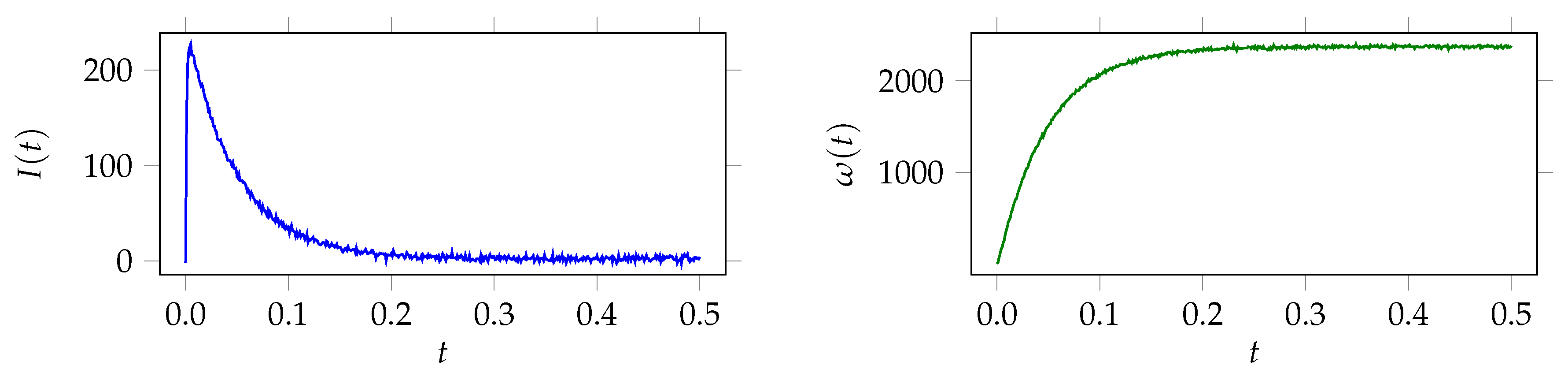
depending only on $R\in \mathcal{X}$. Synthetic measurements for a fixed reference value $R_0=0.1$ are created by $\mathit{y}:=\mathcal{G}\left(R_0\right)+\mathit{\epsilon }$, where $\mathit{\epsilon }:=[{\mathit{\epsilon }}_I,{\mathit{\epsilon }}_{\omega }]$ is a realization of $\mathcal{N}(0,\mathsf{\Sigma })$, with covariance $\mathsf{\Sigma }\in {\mathbb{R}}^{2M\times 2M}$. For independent and identically distributed (iid) measurement noise for current and angular velocity at each time step let $\mathsf{\Sigma }:=diag({\sigma }_I^2{\mathit{I}}_M,{\sigma }_{\omega }^2{\mathit{I}}_M)$, with ${\sigma }_{I,\omega }>0$. Figure 1 displays a measurement of I and $\omega$ with ${\sigma }_{I,0}=2,{\sigma }_{\omega ,0}=10$.

Figure 1. Noisy synthetic measurements of electric current $I\left(t\right)$ and angular velocity $\omega \left(t\right)$.

As the goal of this work is to learn about model discrepancy an artificial model error $\varphi \in \mathbb{R}$ is introduced into $J\dot{\omega }\left(t\right)=\varphi c_{g}I\left(t\right)-d\omega \left(t\right)+T_L$. Let ${\mathcal{G}}_{\varphi }\left(R\right)$ be the numerical approximation of the model for a given $\varphi$ and denote it as simulation model. Obviously, $\mathcal{G}={\mathcal{G}}_{\varphi }\iff \varphi =1$. $\varphi \ne 1$ can be interpreted as missing physics, i.e. by damping or amplifying a part of the equation, or as a misspecified model. Define the discrepancy $\mathit{d}\left(R\right)=[{\mathit{d}}_I,{\mathit{d}}_{\omega }]\left(R\right):=\mathcal{G}\left(R_0\right)-{\mathcal{G}}_{\varphi }\left(R\right)\in {\mathbb{R}}^{2M}$ and the noisy discrepancy ${\mathit{d}}^{\mathit{\epsilon }}\left(R\right)=[{\mathit{d}}_I^{\mathit{\epsilon }},{\mathit{d}}_{\omega }^{\mathit{\epsilon }}]\left(R\right):=\mathit{y}-{\mathcal{G}}_{\varphi }\left(R\right)\in {\mathbb{R}}^{2M}$. Denote for $\varphi =0.9$ the reference discrepancies by ${\mathit{d}}_0:=\mathit{d}\left(R_0\right)$ and ${\mathit{d}}_0^{\mathit{\epsilon }}:={\mathit{d}}^{\mathit{\epsilon }}\left(R_0\right)$.

3. Bayesian Inference Solution Process

Consider the inverse problem of finding an $R\in \mathcal{X}$ such that $\mathit{y}={\mathcal{G}}_{\varphi }\left(R\right)$, where $\mathit{y}\in {\mathbb{R}}^{2M}$ are noisy measurements and ${\mathcal{G}}_{\varphi }$ is the simulation model containing an artificial model error $\varphi$. The goal here is not just to infer an optimal $R\in \mathcal{X}$, but also one that is as close as possible to the reference $R_0$, i.e., the true physical value, which was used to create the measurements $\mathit{y}$. Following [22] we introduce two Bayesian models that differ in their complexity. The simpler model only considers measurement noise, whereas the more complex model considers model discrepancy additionally.

3.1. Bayesian Model 1 (BM1): Measurement Noise

As the measurements $\mathit{y}$ are noisy, additive noise $\mathit{\epsilon }=[{\mathit{\epsilon }}_I,{\mathit{\epsilon }}_{\omega }]\in {\mathbb{R}}^{2M}$ is added to the simulation model. Here, ${\mathit{\epsilon }}_I,{\mathit{\epsilon }}_{\omega }$ are considered as zero mean Gaussian $\mathcal{N}(\mathbf{0},{\sigma }_I^2{\mathit{I}}_M)$ and $\mathcal{N}(0,{\sigma }_{\omega }^2{\mathit{I}}_M)$ with unknown standard deviations ${\sigma }_I,{\sigma }_{\omega }>0$, respectively. The Bayesian model 1 (BM1) is

$$\begin{array}{c}\hfill \mathit{y}={\mathcal{G}}_{\varphi }\left(R\right)+\mathit{\epsilon }({\sigma }_I,{\sigma }_{\omega }).\end{array}$$

(4)

Hence, the likelihood is $\mathit{y}|R,{\sigma }_I,{\sigma }_{\omega }\sim \mathcal{N}({\mathcal{G}}_{\varphi }\left(R\right),\mathsf{\Sigma }({\sigma }_I,{\sigma }_{\omega }))$, with $\mathsf{\Sigma }({\sigma }_I,{\sigma }_{\omega })=diag({\sigma }_I^2{\mathit{I}}_M,{\sigma }_{\omega }^2{\mathit{I}}_M)$. By expressing a-priori knowledge in terms of a prior probability density function $\pi (R,{\sigma }_I,{\sigma }_{\omega })=\pi \left(R\right)\pi \left({\sigma }_I\right)\pi \left({\sigma }_{\omega }\right)$, Bayes’ formula yields for the posterior probability density $\pi (R,{\sigma }_I,{\sigma }_{\omega }|\mathit{y})\sim \pi \left(\mathit{y}\right|R,{\sigma }_I,{\sigma }_{\omega })\pi (R,{\sigma }_I,{\sigma }_{\omega })$. The $\pi \left({\sigma }_I\right),\pi \left({\sigma }_{\omega }\right)$ are defined as uninformative Inverse Gamma distributions $InvGamma(1,1)$. This is a common choice for conjugate priors of scale parameters in Bayesian statistics [4], in particular for a Gaussian likelihood with given mean.

3.2. Bayesian Model 2 (BM2): Measurement Noise and Model Discrepancy

BM2 extends BM1 by considering model discrepancy with an additive term $\mathit{\delta }=[{\mathit{\delta }}_I,{\mathit{\delta }}_{\omega }]\in {\mathbb{R}}^{2M}$, additionally to iid measurement noise. Note that this is already the discretized version and ${\mathit{\delta }}_I=[{\delta }_I\left(t_0\right),\cdots ,{\delta }_I\left(t_M\right)]$, ${\mathit{\delta }}_{\omega }=[{\delta }_{\omega }\left(t_1\right),\cdots ,{\delta }_{\omega }\left(t_M\right)]$ are vectors of the, yet to define, model discrepancy terms ${\delta }_I,{\delta }_{\omega }:D\to \mathbb{R}$ evaluated at $t_i,i=1,\cdots ,M$. Omitting the superscripts for a moment, we now assume that $\delta \in L^2\left(D\right)$. Let ${\left\{p_j\right\}}_{j\in \mathbb{N}}\subseteq L^2\left(D\right)$ be a basis of functions $p_j:D\to \mathbb{R}$ dense in $L^2\left(D\right)$. Then $\delta$ can be represented by the expansion $\delta \left(t\right)={\sum }_{j=0}^{\infty }{a}_j{p}_j\left(t\right).$ For practicability reasons the expansion is truncated after a $K\in \mathbb{N}$. Such an truncated expansion was also used in [22]. With this let, for the truncation parameter $K\in \mathbb{N}$, the truncated functional expansions

$$\begin{array}{c}\hfill {\delta }_I^K\left(t\right)=\sum _{j=0}^K{a}_j^{\left(I\right)}{p}_j\left(t\right),{\delta }_{\omega }^K\left(t\right)=\sum _{j=0}^K{a}_j^{\left(\omega \right)}{q}_j\left(t\right),\end{array}$$

(5)

be approximative models for the model discrepancy terms ${\delta }_I,{\delta }_{\omega }$. The bases ${\left\{p_j\right\}}_{j=0,\cdots ,K}$ and ${\left\{q_j\right\}}_{j=0,\cdots ,K}$ are not necessarily identical. Note that each expansion could be truncated with own truncation parameters $K_I,K_{\omega }$, but for notational convenience and due to later usage we stick to $K=K_I=K_{\omega }$. Let $\mathit{a}=[{\mathit{a}}^{\left(I\right)},{\mathit{a}}^{\left(\omega \right)}]=[a_0^{\left(I\right)},\cdots ,a_K^{\left(I\right)},a_0^{\left(\omega \right)},\cdots ,a_K^{\left(\omega \right)}]\in {\mathbb{R}}^{2K+2}$ be the coefficient vector and ${\mathit{\delta }}_I^K\left(\mathit{a}\right)=[{\delta }_I^K\left(t_0\right),\cdots ,{\delta }_I^K\left(t_M\right)]$, ${\mathit{\delta }}_{\omega }^K\left(\mathit{a}\right)=[{\delta }_{\omega }^K\left(t_1\right),\cdots ,{\delta }_{\omega }^K\left(t_M\right)]$. Hence ${\mathit{\delta }}^K\left(\mathit{a}\right)=[{\mathit{\delta }}_I^K,{\mathit{\delta }}_{\omega }^K]\left(\mathit{a}\right)\in {\mathbb{R}}^{2M}$ denotes the approximation of the true underlying model discrepancy $\mathit{\delta }$.The Bayesian model 2 (BM2) is

$$\begin{array}{c}\hfill \mathit{y}={\mathcal{G}}_{\varphi }\left(R\right)+{\mathit{\delta }}^K\left(\mathit{a}\right)+\mathit{\epsilon }({\sigma }_I,{\sigma }_{\omega }).\end{array}$$

(6)

The number of unknown parameters is $3+2K+2$. With the additional unknown coefficients $\mathit{a}$, the prior probability density function is defined as $\pi (R,{\sigma }_I,{\sigma }_{\omega },\mathit{a})=\pi \left(R\right)\pi \left({\sigma }_I\right)\pi \left({\sigma }_{\omega }\right)\pi \left(\mathit{a}\right),$ where $\pi \left(\mathit{a}\right)={\prod }_{j=0}^K\pi \left(a_j^{\left(I\right)}\right)\pi \left(a_j^{\left(\omega \right)}\right)$. The prior distributions for $\pi \left({\sigma }_I\right)$ and $\pi \left({\sigma }_{\omega }\right)$ are specified as above. Now, with the likelihood $\mathit{y}|R,{\sigma }_I,{\sigma }_{\omega },\mathit{a}\sim \mathcal{N}({\mathcal{G}}_{\varphi }\left(R\right)+{\mathit{\delta }}^K\left(\mathit{a}\right),\mathsf{\Sigma }({\sigma }_I,{\sigma }_{\omega })),$ the posterior is given by ${\pi }^K(R,{\sigma }_I,{\sigma }_{\omega },\mathit{a}|\mathit{y})\sim \pi \left(\mathit{y}\right|R,{\sigma }_I,{\sigma }_{\omega },\mathit{a})\pi (R,{\sigma }_I,{\sigma }_{\omega },\mathit{a}),$ where ${\pi }^K$ denotes the dependence on K.

Choosing basis functions and priors for the coefficients: If knowledge about the discrepancy is available, this should be modeled accordingly by defining an appropriate prior distribution for $\mathit{\delta }$, i.e., in the case of ${\mathit{\delta }}^K\left(\mathit{a}\right)$ appropriate choices for $\mathit{a},K$ and ${\left\{p_j\right\}}_{j=0,\cdots ,K}\subset L^2\left(D\right)$. However, in general this knowledge is not available and some modeling assumptions need to be made. With the assumption that $\mathit{\delta }$ is rather smooth, orthonormal polynomials $p_j:D\to \mathbb{R}$ with $deg\left(p_j\right)=j$ are a reasonable choice. As [22], we also opt for Legendre polynomials that are orthogonal to a constant weight. In [22] they argue about the prior for the coefficients $\pi \left(a_j^{\left(I\right)}\right),\pi \left(a_j^{\left(\omega \right)}\right)$ and decide for zero mean Laplace distribution $Laplace(0,b)$ with the arbitrary choice of $b=10$. It assigns the highest probability around zero and decays exponentially towards the tails, see [25].

Choosing the truncation parameter K: With the choice of Legendre polynomials K corresponds to the maximum polynomial degree. This K determines the complexity of the model discrepancy term ${\mathit{\delta }}^K\left(\mathit{a}\right)$. Important factors in order to specify the model discrepancy term complexity are: accuracy, computational costs, bias-variance tradeoff and non-identifiability. An optimal K should be large enough such that ${\mathit{\delta }}^K\left(\mathit{a}\right)$ is accurate enough to approximate the underlying discrepancy correct, but at the same time it should be as small as possible since a large K increases the number of unknown parameters and consequently computational costs. Furthermore, a large K might yield non-identifiability of all unknowns, as the prior of ${\mathit{\delta }}^K\left(\mathit{a}\right)$ gets non-informative. In [18] they state that in order to infer model discrepancy and model parameters at the same time, at least for one of those an informative prior must be given. The term bias-variance tradeoffdescribes the fact that with increasing model complexity K the bias of an estimator decreases, but at the same time the variance increases with the model complexity [26]. Consequently, the overall error as sum of squared bias and variance is minimal for an optimal model complexity.

Taking all these factors into account the approach in this work on how to find an optimal K is following: Start with an initial $K=K_0\in \mathbb{N}$ and increase K iteratively until the marginal posterior distribution ${\pi }^K({\sigma }_I,{\sigma }_{\omega }|\mathit{y})$ of the noise standard deviations stabilizes. i.e., that some distance $D({\pi }^K({\sigma }_I,{\sigma }_{\omega }|\mathit{y}),{\pi }^{K+L}({\sigma }_I,{\sigma }_{\omega }|\mathit{y}))<tol$ for a given tolerance $tol>0$ and $L\in \mathbb{N}$. Then select the K such that this condition holds. Why is this sufficient? If a model discrepancy is present in BM1, then the noise term is the only instance to capture it. As the noise term is modeled with zero mean, the standard deviation might be overestimated consequently. By adding the model discrepancy term in BM2 captures a fraction of the model discrepancy. As a consequence, the noise term $\mathit{\epsilon }$ needs to represent only the remaining discrepancy and is estimated by a smaller value. If the estimated standard deviation of the noise does not change anymore (within the tolerance) from K to $K+L$ for $L\in \mathbb{N}$ the smallest sufficient K is found. For this K the model discrepancy term ${\mathit{\delta }}^K\left(\mathit{a}\right)$ should represent the underlying model discrepancy best within its current specification and a separation of model uncertainty and measurement uncertainty is achieved.

4. Numerical Results

The numerical results for BM1 and BM2 applied to the electric motor model are presented and compared to the reference. The prior distribution for R is chosen as $\mathcal{N}(R_0,0.2R_0)$. Variations of the prior mean by +/−15% did not influence the upcoming results much, thus simply $R_0$ was chosen as mean. An MH-MCMC implementation of the Python package PyMC3 [7] is used to approximate the posterior distribution probability density function. The marginal posterior moments are empirically approximated using Monte Carlo integration with a certain number of the obtained MH-MCMC samples. In order to compare and evaluate the solutions we define error measures.

Definition 1. 

Define the relative error for a parameter estimate $\widehat{x}$ as ${ϵ}_{rel}\left(x\right)=|\widehat{x}-x_0|/\left|x_0\right|$, where $x_0$ is the reference value. $\widehat{x}$ might be the empirical approximation of the marginal posterior mean $\mathbb{E}\left[x\right|\mathit{y}]$.

Definition 2. 

Let x with $\pi \left(x\right|\mathit{y})$ be an estimation for $x_0\in \mathbb{R}$ and given $\mathit{y}$. The mean square error (MSE) of x is $MSE\left(x\right):=\mathbb{E}\left[{(x-x_0)}^2\right|\mathit{y}]=Bias{\left(x\right)}^2+V\left[x\right|\mathit{y}]$, with $Bias\left(x\right)=(\mathbb{E}\left[x\right|\mathit{y}]-x_0)$. The mean is with respect to $\pi \left(x\right|\mathit{y})$. In case of ${\pi }^K\left(x\right|\mathit{y})$ depending on K write $MS{E}_K\left(x\right)={\mathbb{E}}_K\left[{(x-x_0)}^2\right|\mathit{y}]=Bia{s}_K{\left(x\right)}^2+V_K\left[x\right|\mathit{y}]$.

4.1. Results Bayesian Model 1

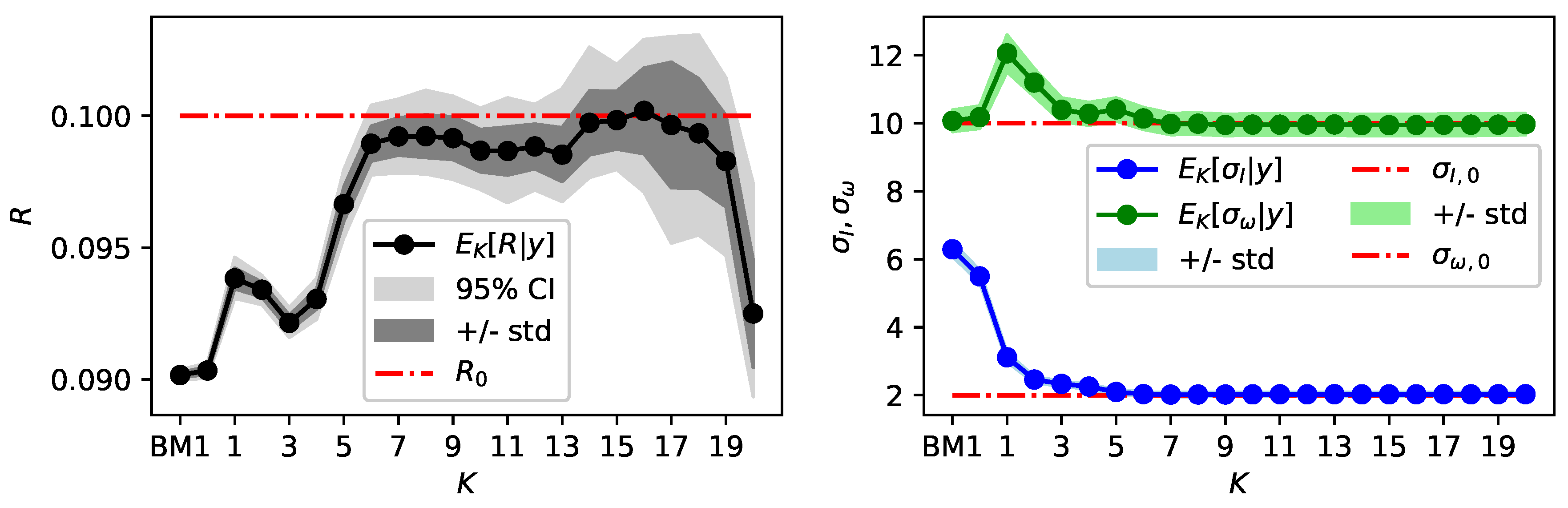
In Figure 2 the index BM1 denotes marginal posterior moments for parameters $R,{\sigma }_I$ and ${\sigma }_{\omega }$ obtained with BM1 in comparison to the reference and BM2. With respect to a burn in phase, only the last 700 samples of three independently sampled Markov chains, each of total length 1500, are used to obtain the results. The marginal posterior distribution for ${\sigma }_{\omega }$ is close to the reference, but for R and ${\sigma }_I$ the marginal posteriors concentrate at values different to the references and do not even assign a significant probability to the references. The marginal posterior mean values of $R,{\sigma }_I$ and ${\sigma }_{\omega }$ and their respective relative error with respect to the reference are displayed in Table 1.

Figure 2. Results obtained with BM1 (noted by index BM1) and BM2 for $K=0,\cdots ,20$. Moments of the marginal posterior distributions of R are displayed on the left and moments of ${\sigma }_I,{\sigma }_{\omega }$ on the right.

Table 1. Marginal posterior mean and relative error of parameters $R,{\sigma }_I$ and ${\sigma }_{\omega }$ for BM1 and BM2 with $K=9$. The relative errors are with respect to the reference values $R_0=0.1,{\sigma }_{I,0}=2$, and ${\sigma }_{\omega ,0}=10$.

	Marginal Posterior Mean			Relative Error
	$\widehat{\mathit{R}}$	${\widehat{\mathit{\sigma }}}_{\mathit{I}}$	${\widehat{\mathit{\sigma }}}_{\mathit{\omega }}$	${\mathit{ϵ}}_{\mathit{rel}}\left(\widehat{\mathit{R}}\right)$	${\mathit{ϵ}}_{\mathit{rel}}\left({\widehat{\mathit{\sigma }}}_{\mathit{I}}\right)$	${\mathit{ϵ}}_{\mathit{rel}}\left({\widehat{\mathit{\sigma }}}_{\mathit{\omega }}\right)$
BM1	9.03 × ${10}^{-2}$	6.29 × ${10}^0$	1.03 × ${10}^1$	9.66 × ${10}^{-2}$	2.14 × ${10}^0$	2.79 × ${10}^{-2}$
BM2 ($K=9$)	9.92 × ${10}^{-2}$	2.02 × ${10}^0$	9.95 × ${10}^0$	8.48 × ${10}^{-3}$	1.03 × ${10}^{-2}$	4.89 × ${10}^{-3}$

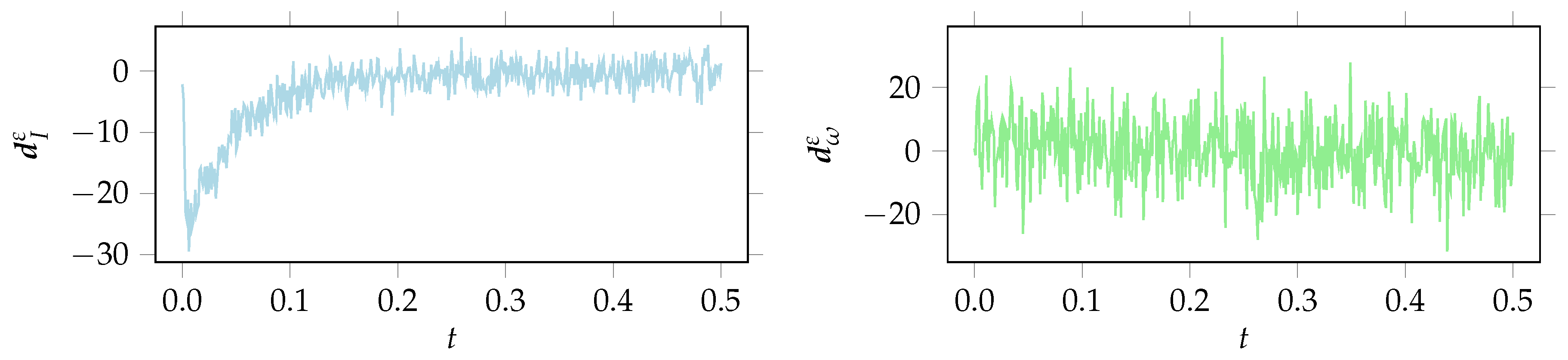
The noisy discrepancy ${\mathit{d}}^{\mathit{\epsilon }}\left(\widehat{R}\right)$ for $\widehat{R}$ is displayed in Figure 3. (Remark: For simplicity the mean $\mathbb{E}\left[{\mathit{d}}^{\mathit{\epsilon }}\left(R\right)\right|\mathit{y}]=\mathit{y}-\mathbb{E}\left[{\mathcal{G}}_{\varphi }\left(R\right)\right|\mathit{y}]\approx \mathit{y}-{\mathcal{G}}_{\varphi }\left(\mathbb{E}\left[R\right|\mathit{y}]\right)$ is approximated by assuming linearity for ${\mathcal{G}}_{\varphi }$ in a neighborhood of $\widehat{R}$.) For $\omega$ this is basically the measurement noise, since $\mathbb{E}\left[{\mathit{d}}_{\omega }^{\mathit{\epsilon }}\right]\approx 0$ and $V{\left[{\mathit{d}}_{\omega }^{\mathit{\epsilon }}\right]}^{1/2}=10.18\approx {\sigma }_{\omega ,0}\approx {\widehat{\sigma }}_{\omega }$. But for ${\mathit{d}}_I^{\mathit{\epsilon }}$ there is some discrepancy, at least in the first half of the time interval, different to measurement noise. Calculating the empirical standard deviation for a fixed zero mean ${\sigma }_I^{†}:=\frac{1}{M-1}{\sum }_{i=1}^M{\left({\mathit{d}}_I^{\mathit{\epsilon }}{\left(\widehat{R}\right)}_i\right)}^2$, where ${\mathit{d}}_I^{\mathit{\epsilon }}{\left(\widehat{R}\right)}_i$ denotes the i-th component of ${\mathit{d}}_I^{\mathit{\epsilon }}\left(\widehat{R}\right)$, one obtains ${\sigma }_I^{†}=6.23\approx {\widehat{\sigma }}_I$. The obtained value corresponds to the overestimated marginal posterior distribution of ${\sigma }_I$ that centers around a similar value, see Figure 2 and Table 1. Obviously, BM1 leads to biased and overconfident parameter estimates.

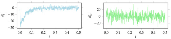
Figure 3. Remaining discrepancy ${\mathit{d}}^{\mathit{\epsilon }}\left(\widehat{R}\right)=[{\mathit{d}}_I^{\mathit{\epsilon }},{\mathit{d}}_{\omega }^{\mathit{\epsilon }}]\left(\widehat{R}\right)=\mathit{y}-{\mathcal{G}}_{\varphi }\left(\widehat{R}\right)$, for $\widehat{R}$ obtained with BM1.

4.2. Results Bayesian Model 2

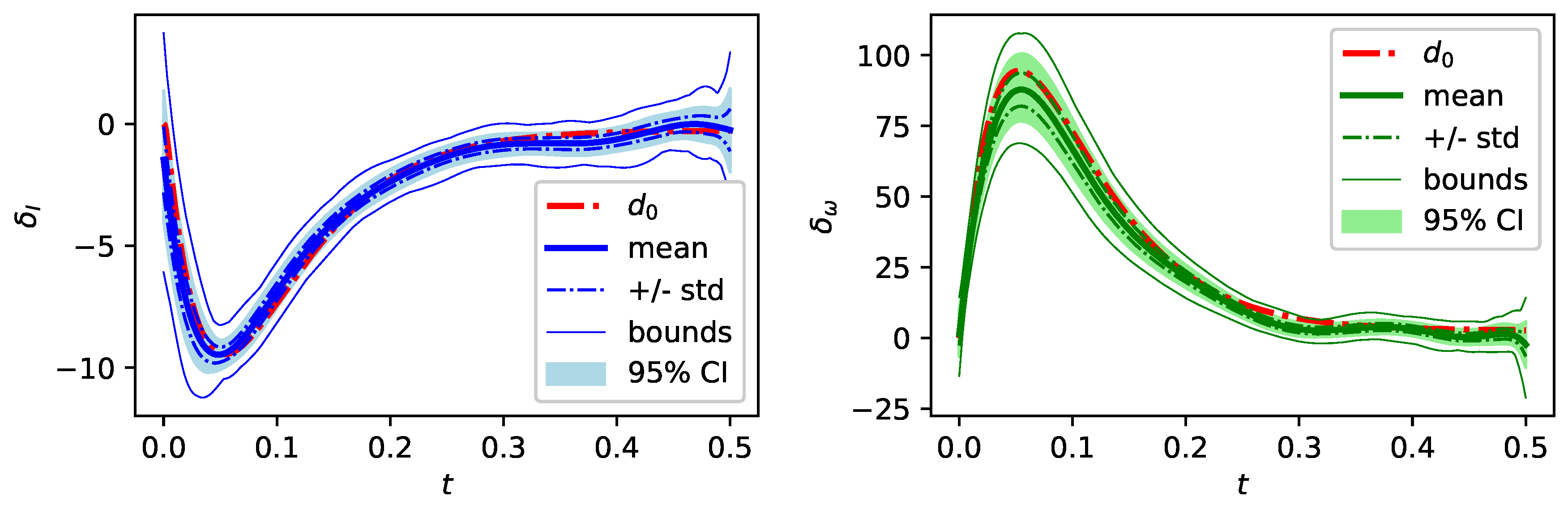
Figure 2 also displays moments of the marginal posterior distributions of $R,{\sigma }_I$ and ${\sigma }_{\omega }$, obtained via BM2 for $K=0,\cdots ,20$. For each K the last $0.4\times {10}^5$ samples of three independently sampled Markov chains of length ${10}^5$ are used to approximate the moments. In contrast to BM1 a larger number of MH-MCMC samples is required for convergence, due to an increased number of unknowns in BM2. For comparison, the index BM1 in the following figures denotes results without $\mathit{\delta }$. Following the guideline specified in Section 3 the marginal posterior distributions of the noise standard deviations of ${\sigma }_I$ and ${\sigma }_{\omega }$ in Figure 2 are considered to pick an appropriate K. Both marginal posterior distributions ${\pi }^K\left({\sigma }_I\right|\mathit{y})$ and ${\pi }^K\left({\sigma }_{\omega }\right|\mathit{y})$ stabilize for $K\ge 7$ and are almost identical for $K\ge 9$, considering mean and standard deviation of the marginal posterior distribution. This indicates that $K=9$ is a sufficient polynomial degree and increasing K further does not improve the results with the current specification of the model discrepancy term. Figure 4 displays for $K=9$ the concentration of the posterior distribution of ${\mathit{\delta }}^K\left(\mathit{a}\right)=[{\mathit{\delta }}_I^K,{\mathit{\delta }}_{\omega }^K]\left(\mathit{a}\right)$ around the reference discrepancy ${\mathit{d}}_0$.

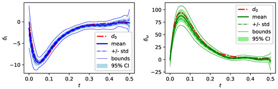
Figure 4. Posterior moments of model discrepancy ${\mathit{\delta }}^K\left(\mathit{a}\right)=[{\mathit{\delta }}_I^K,{\mathit{\delta }}_{\omega }^K]\left(\mathit{a}\right)$ for $K=9$ in comparison to the reference discrepancy ${\mathit{d}}_0=[{\mathit{d}}_{I,0},{\mathit{d}}_{\omega ,0}]$.

The relative error $nBia{s}_K({\mathit{\delta }}_{*}^K-d_{0,*})/\parallel d_{0,*}\parallel$ is 1.0 ×${10}^{-1}$ for I and 9.2 ×${10}^{-2}$ for $\omega$. Also the marginal posterior distribution of R concentrates close to the reference value and the relative error of the posterior mean reduces around one order of magnitude compared to the result of BM1, see Table 1. Also, both noise standard deviations concentrate around the reference and significantly improve in relative errors compared to BM1. Overall, the posterior distribution of ${\mathcal{G}}_{\varphi }\left(R\right)+{\mathit{\delta }}^K\left(\mathit{a}\right)+\mathit{\epsilon }$ yields a good approximation of the measurements $\mathit{y}$ with only a small variance band. Figure 2 shows that for $K=6,\cdots ,19$ the marginal posterior mean of R roughly stabilizes in some kind of a plateau close to the reference $R_0$, but the posterior standard deviation increases with K. For $K=0,\cdots ,5$ the model discrepancy term ${\mathit{\delta }}^K\left(\mathit{a}\right)$ is not flexible enough to approximate the underlying discrepancy appropriate enough. As a consequence, the standard deviations of the measurement noise are overestimated and the estimation of the parameter R is still biased for those values of K.

Adding on this, Figure 5 displays $Bia{s}_K$, variance $V_K$ and $MS{E}_K$ of R. The MSE of R is minimal around $K=7,8,9$ and $K=15$, indicating those values as an optimal model complexity and backing up the decision of $K=9$ as sufficient polynomial degree. Figure 5 largely corresponds to the bias-variance tradeoff, since the variance increases with K and the bias decreases with K, at least until $K=15$. For $K\ge 15$ the bias increases as non-identifiability occurs additionally. Especially for $K=20$ overfitting and non-identifiability can be observed as the posterior distribution of R is spread out and biased, see Figure 2. For complimentary numerical results (e.g., posterior moments of ${\mathit{\delta }}^K\left(\mathit{a}\right)$ for $K=20$) see the accompanying preprint of this work [27].

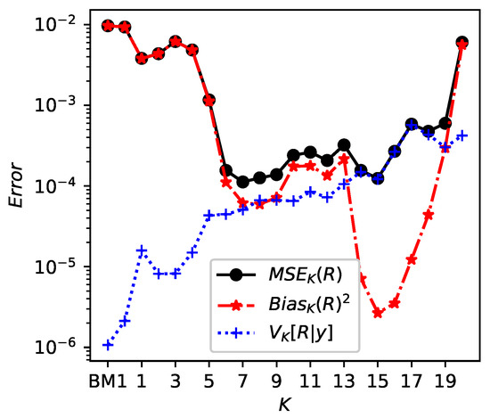
Figure 5. Bias-variance tradeoff: Bias $Bia{s}_K\left(R\right)$, variance $V_K\left[R\right|\mathit{y}]$ and mean square error $MS{E}_K\left(R\right)$ of R with respect to $R_0$, depending on K, for $K=0,\cdots ,20$ from BM2. The index BM1 denotes the previous results without $\mathit{\delta }$, obtained via Bayesian model 1.

5. Conclusions

In this work a method to infer model parameters and model discrepancy is considered and applied to synthetic measurement data of an electric motor. The suggested Bayesian model 2 (BM2) considers measurement noise and model discrepancy, in order to separate these two sources of uncertainty and improve physical parameter estimation. The model discrepancy term is modeled as a truncated polynomial expansion ${\mathit{\delta }}^K\left(\mathit{a}\right)$ with unknown coefficients $\mathit{a}$ and an maximum polynomial degree K. A discussion and a guideline on how to define appropriate model discrepancy term complexity, i.e., here the maximum polynomial degree K, based on the marginal posterior distribution of measurement noise standard deviation is presented. The framework applied to the electric motor showed promising perspectives by an improved estimation of the model parameters. Furthermore a good approximation of the a-priori unknown model discrepancy is learned with BM2 for a sufficient maximum polynomial degree $K=9$. An appropriate choice of K is crucial. For K too small the accuracy of ${\mathit{\delta }}^K\left(\mathit{a}\right)$ is not sufficient and estimation is just slightly improved. If K is too large the prior contains to less information about the reference discrepancy and consequently the posterior distribution does not converge anymore. Consequently, in order to identify both, the underlying parameter value and the reference discrepancy of the test scenario, it is important to find an optimal K and with this formulate at least for one of the unknowns a prior containing some information about the reference.

Next steps are to apply this approach to higher dimensional problems and further to real field data to test its capabilities. Then, as real data implies a more complex simulator, surrogate modeling will be mandatory to leverage computational expenses. Additionally, evidence approximation could be an another criteria to select a Bayesian model, which will be considered in future work.

References

- Kaipio, J.; Somersalo, E. Statistical and Computational Inverse Problems; Applied Mathematical Sciences; Springer Science+Business Media, Inc.: New York, NY, USA, 2005. [Google Scholar]
- Stuart, A.M. Inverse problems: A Bayesian perspective. Acta Numer. 2010, 19, 451–559. [Google Scholar] [CrossRef]
- Dashti, M.; Stuart, A.M. The Bayesian Approach to Inverse Problems. In Handbook of Uncertainty Quantification; Ghanem, R., Higdon, D., Owhadi, H., Eds.; Springer: Cham, Switzerland, 2017; pp. 311–428. [Google Scholar]
- Gelman, A.; Carlin, J.B.; Stern, H.S.; Dunson, D.B.; Vehtari, A.; Rubin, D.B.; Stern, H.S. Bayesian Data Analysis, 3rd ed.; Texts in Statistical Science Series; CHAPMAN & HALL/CRC and CRC Press: Boca Raton, FL, USA, 2013. [Google Scholar]
- Sullivan, T.J. Introduction to Uncertainty Quantification; Texts in Applied Mathematics 0939-2475; Springer: Berlin, Germany, 2015; Volume 63. [Google Scholar]
- Hastings, W.K. Monte Carlo Sampling Methods Using Markov Chains and Their Applications. Biometrika 1970, 57, 97. [Google Scholar] [CrossRef]
- Salvatier, J.; Wiecki, T.V.; Fonnesbeck, C. Probabilistic programming in Python using PyMC3. PeerJ Comput. Sci. 2016, 2, e55. [Google Scholar] [CrossRef]
- Schillings, C.; Schwab, C. Scaling limits in computational Bayesian inversion. ESAIM Math. Model. Numer. Anal. 2016, 50, 1825–1856. [Google Scholar] [CrossRef]
- Sprungk, B. Numerical Methods for Bayesian Inference in Hilbert Spaces, 1st ed.; Universitätsverlag der TU Chemnitz: Chemnitz, Germany, 2018. [Google Scholar]
- Hoffman, M.D.; Gelman, A. The No-U-turn sampler: adaptively setting path lengths in Hamiltonian Monte Carlo. J. Mach. Learn. Res. 2014, 15, 1593–1623. [Google Scholar]
- Xiu, D.; Karniadakis, G.E. The Wiener-Askey polynomial chaos for stochastic differential equations. SIAM J. Sci. Comput. 2002, 24, 619–644. [Google Scholar] [CrossRef]
- Glaser, P.; Schick, M.; Petridis, K.; Heuveline, V. Comparison between a Polynomial Chaos surrogate model and Markov Chain Monte Carlo for inverse Uncertainty Quantification based on an electric drive test bench. In Proceedings of the ECCOMAS Congress 2016, Crete Island, Greece, 5–10 June 2016. [Google Scholar]
- Kennedy, M.C.; O’Hagan, A. Bayesian calibration of computer models. J. R. Stat. Soc. Ser. B Stat. Methodol. 2001, 63, 425–464. [Google Scholar] [CrossRef]
- Rasmussen, C.E.; Williams, C.K. Gaussian Process for Machine Learning; MIT Press: Cambridge, MA, USA, 2006. [Google Scholar]
- Arendt, P.D.; Apley, D.W.; Chen, W. Quantification of Model Uncertainty: Calibration, Model Discrepancy, and Identifiability. J. Mech. Des. 2012, 134, 100908. [Google Scholar] [CrossRef]
- Arendt, P.D.; Apley, D.W.; Chen, W.; Lamb, D.; Gorsich, D. Improving Identifiability in Model Calibration Using Multiple Responses. J. Mech. Des. 2012, 134, 100909. [Google Scholar] [CrossRef]
- Paulo, R.; García-Donato, G.; Palomo, J. Calibration of computer models with multivariate output. Comput. Stat. Data Anal. 2012, 56, 3959–3974. [Google Scholar] [CrossRef]
- Brynjarsdóttir, J.; O’Hagan, A. Learning about physical parameters: The importance of model discrepancy. Inverse Probl. 2014, 30, 114007. [Google Scholar] [CrossRef]
- Tuo, R.; Wu, C.F.J. Efficient calibration for imperfect computer models. Ann. Stat. 2015, 43, 2331–2352. [Google Scholar] [CrossRef]
- Tuo, R.; Jeff Wu, C.F. A Theoretical Framework for Calibration in Computer Models: Parametrization, Estimation and Convergence Properties. SIAM/ASA J. Uncertain. Quantif. 2016, 4, 767–795. [Google Scholar] [CrossRef]
- Plumlee, M. Bayesian Calibration of Inexact Computer Models. J. Am. Stat. Assoc. 2016, 112, 1274–1285. [Google Scholar] [CrossRef]
- Nagel, J.B.; Rieckermann, J.; Sudret, B. Uncertainty Quantification in Urban Drainage Simulation: Fast Surrogates for Sensitivity Analysis and Model Calibration. 2017. Available online: http://arxiv.org/abs/1709.03283 (accessed on 23 March 2018).
- Toliyat, H.A. (Ed.) Handbook of Electric Motors, 2nd ed.; Electrical and Computer Engineering; Dekker: New York, NY, USA; Basel, Switzerland, 2004; Volume 120. [Google Scholar]
- Wanner, G.; Hairer, E. Solving Ordinary Differential Equations I; Springer: Berlin, Germany, 1991; Volume 1. [Google Scholar]
- Kotz, S.; Kozubowski, T.; Podgorski, K. The Laplace Distribution and Generalizations: A Revisit with Applications to Communications, Economics, Engineering, and Finance; Springer Science & Business Media: Berlin, Germany, 2012. [Google Scholar]
- Hastie, T.; Tibshirani, R.; Friedman, J.H. The Elements of Statistical Learning: Data Mining, Inference, and Prediction, 2nd ed.; Springer Series in Statistics; Springer: New York, NY, USA, 2009. [Google Scholar]
- John, D.; Schick, M.; Heuveline, V. Learning model discrepancy of an electric motor with Bayesian inference. Eng. Math. Comput. Lab 2018. [Google Scholar] [CrossRef]
Publisher’s Note: MDPI stays neutral with regard to jurisdictional claims in published maps and institutional affiliations. |
© 2019 by the authors. Licensee MDPI, Basel, Switzerland. This article is an open access article distributed under the terms and conditions of the Creative Commons Attribution (CC BY) license (https://creativecommons.org/licenses/by/4.0/).