


Efficient UAV Exploration for Large-Scale 3D Environments Using Low-Memory Map

Abstract
:1. Introduction
- A novel representation of the environment is presented to provide the essential information for exploration: only obstacle and frontier information are maintained, requiring less onboard memory. And a method is designed to update the representation immediately whenever new environmental data are received.
- A hierarchical exploration approach incorporating the proposed environmental representation is developed to enable fast planning and generate high-quality exploration paths, allowing for quick responses to environmental changes and improving overall exploration efficiency.
- Comprehensive simulations and real-world experiments demonstrate that the proposed environmental representation is memory-efficient, and the proposed exploration method is able to promptly plan efficient exploration paths in large-scale environments.
2. Related Work
2.1. Autonomous Exploration Methods
2.2. Environmental Representation
3. System Overview
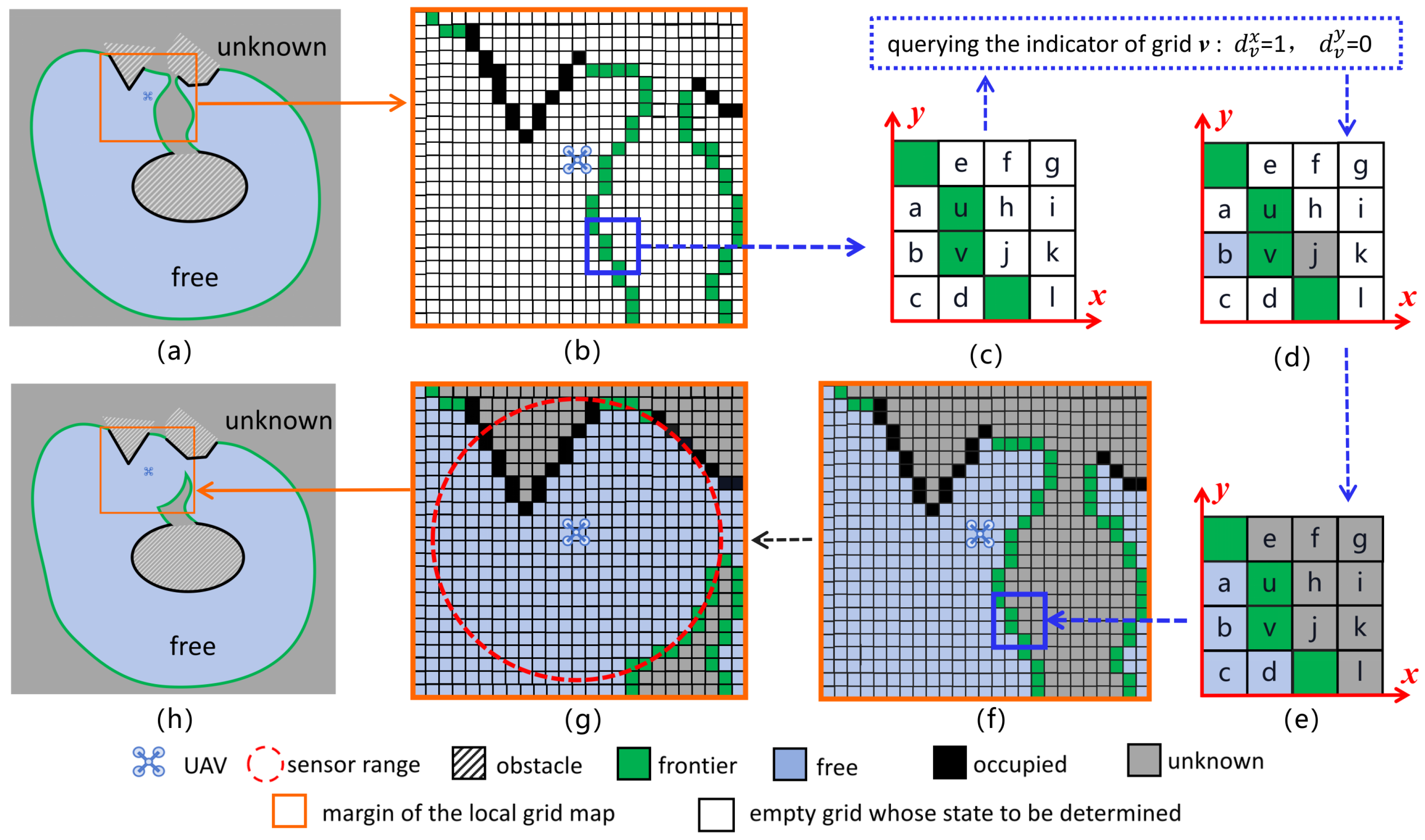
4. A 3D Environmental Representation for Exploration
4.1. Representation of FAOmap
4.2. Data Structure of FAOmap
4.3. Updating of FAOmap
- (1)
- After the UAV moves, the local 3D grid map is centered at the UAV’s current position, and all grids in G are reset to the empty state (the real state has yet to be determined).
- (2)
- Based on the coordinates, the frontiers and the occupied grids in the range of are retrieved from FAOmap and stored in their corresponding grids in , as shown in Figure 4b. And then, they are erased in FAOmap.
- (3)
- The grids in are clustered according to their current states (frontier, occupied, and empty). The possible occupancy states of a grid in are frontier, free, occupied, and unknown, as shown in Figure 2c. Since the frontiers and occupied grids are identified in step 2, the empty grids are free or unknown. The real states of empty grids in the same cluster are determined by the indicators of the frontiers or the occupied grids adjacent to . For example, as shown in Figure 4c–e, supposing that along the positive direction of the x-coordinate, there is a frontier v adjacent to the grid b, which is in cluster . After querying the indicator of grid v, whose value is 1, it can be inferred that the state of grid b is known, according to Figure 2d. However, there are only two types of known grids: free and occupied. But occupied grids have already been identified in step (2), so the real state of grid b is free. Then the real states of all grids in are free. Similarly, the real states of all empty grids in other clusters can be determined.
- (4)
- The occupancy states of all grids in are updated based on newly received data using a ray-cast approach, as in Octomap [38].
- (5)
- All new frontiers and occupied grids in are extracted and added to FAOmap.
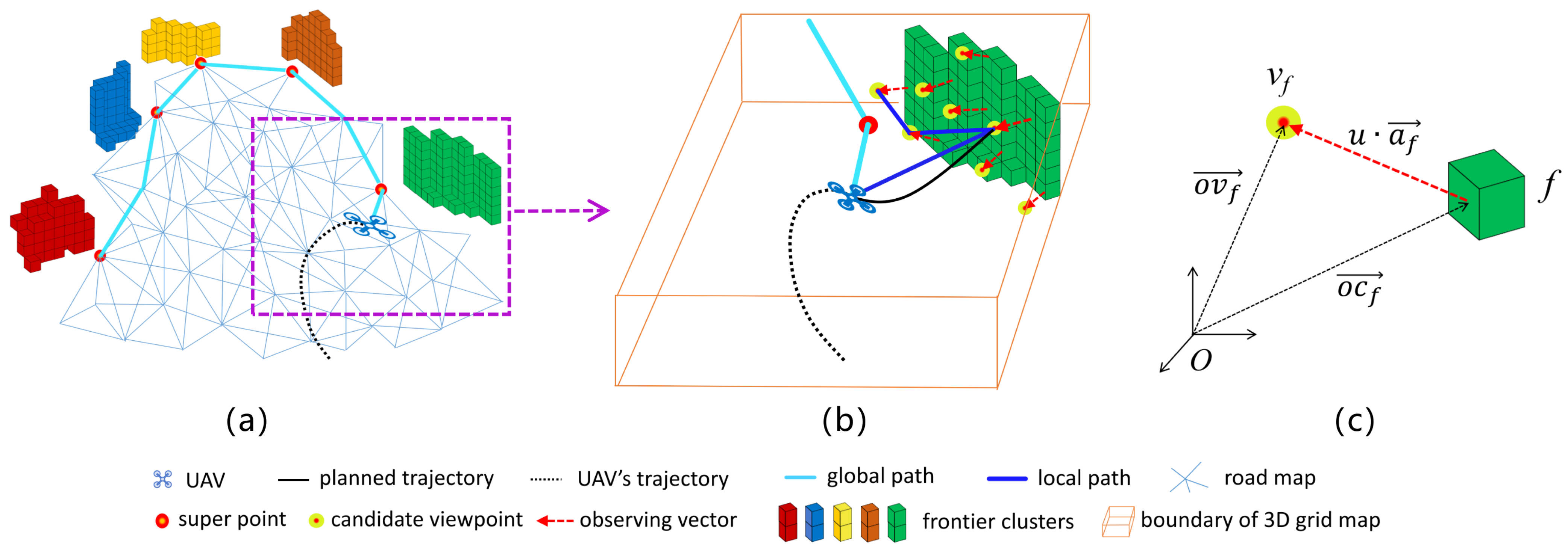
5. Hierarchical Exploration Approach
5.1. Global Planning
5.1.1. Fast Incremental Frontier Clustering
- (1)
- Find all clusters that currently overlap with the local 3D grid map G. If a cluster falls inside the range of G, then delete it (as with the orange cluster in Figure 5a).
- (2)
- For clusters that intersect with the boundary of G, some frontiers in these clusters may no longer be the frontiers after G is updated by newly perceived data. If the number of remaining frontiers in a cluster is less than the threshold , delete the cluster (as with the green cluster in Figure 5); otherwise, retain clusters that consist of remaining frontiers (as with the blue cluster in Figure 5).
- (3)
- Cluster all frontiers that are not yet clustered, including the new frontiers that appear after G is updated and some frontiers from the deleted clusters.

5.1.2. Super Points for Frontier Clusters
5.1.3. Exploration Routes Finding
5.1.4. Road Map for Path Searching
5.2. Local Refinement
5.2.1. Viewpoint Generation
5.2.2. Observation Path Determination
6. Trajectory Optimization
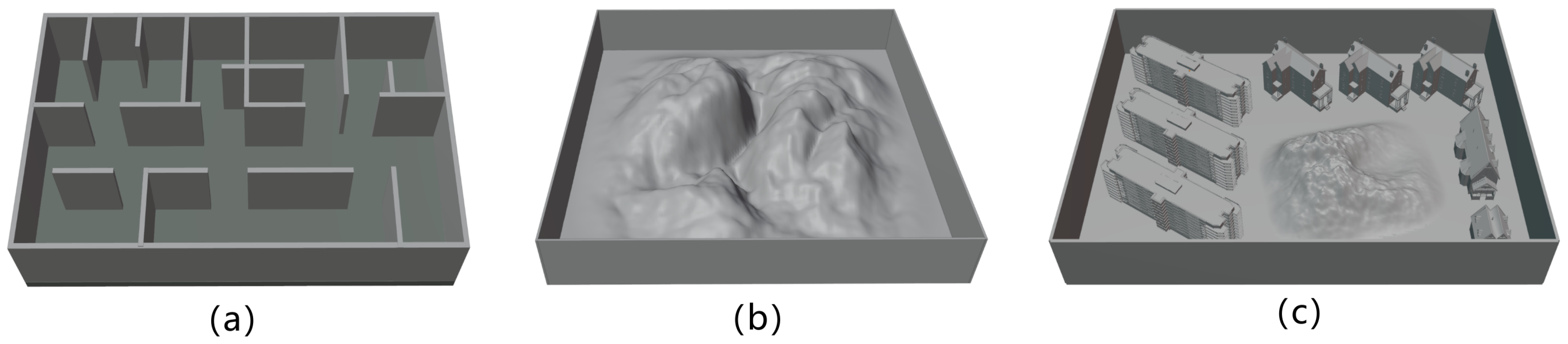
7. Simulation Experiments
7.1. FAOmap Evaluation
7.1.1. Memory Consumption
7.1.2. Update Efficiency
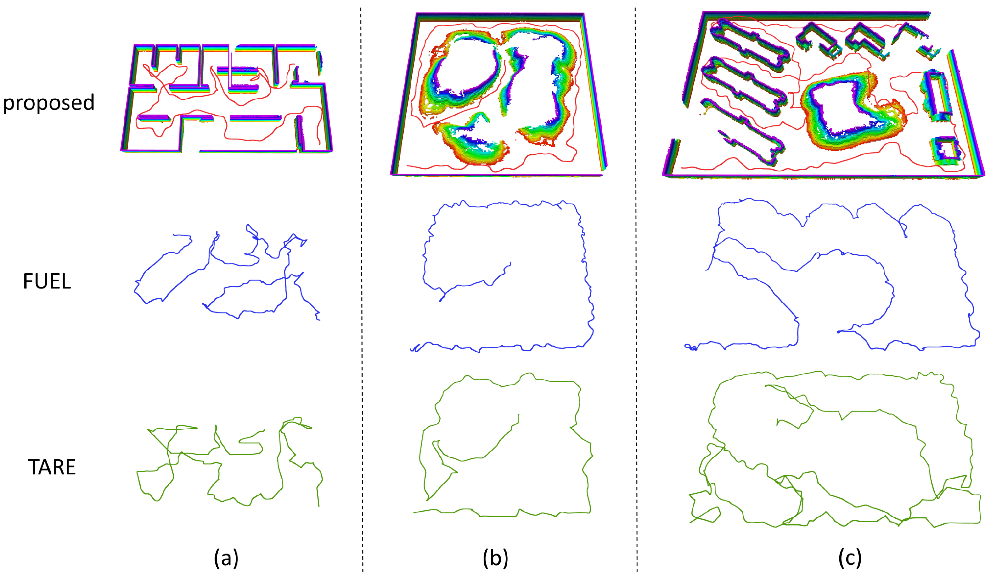
7.2. Exploration Planning Method Evaluation
7.2.1. Computational Efficiency
7.2.2. Exploration Efficiency
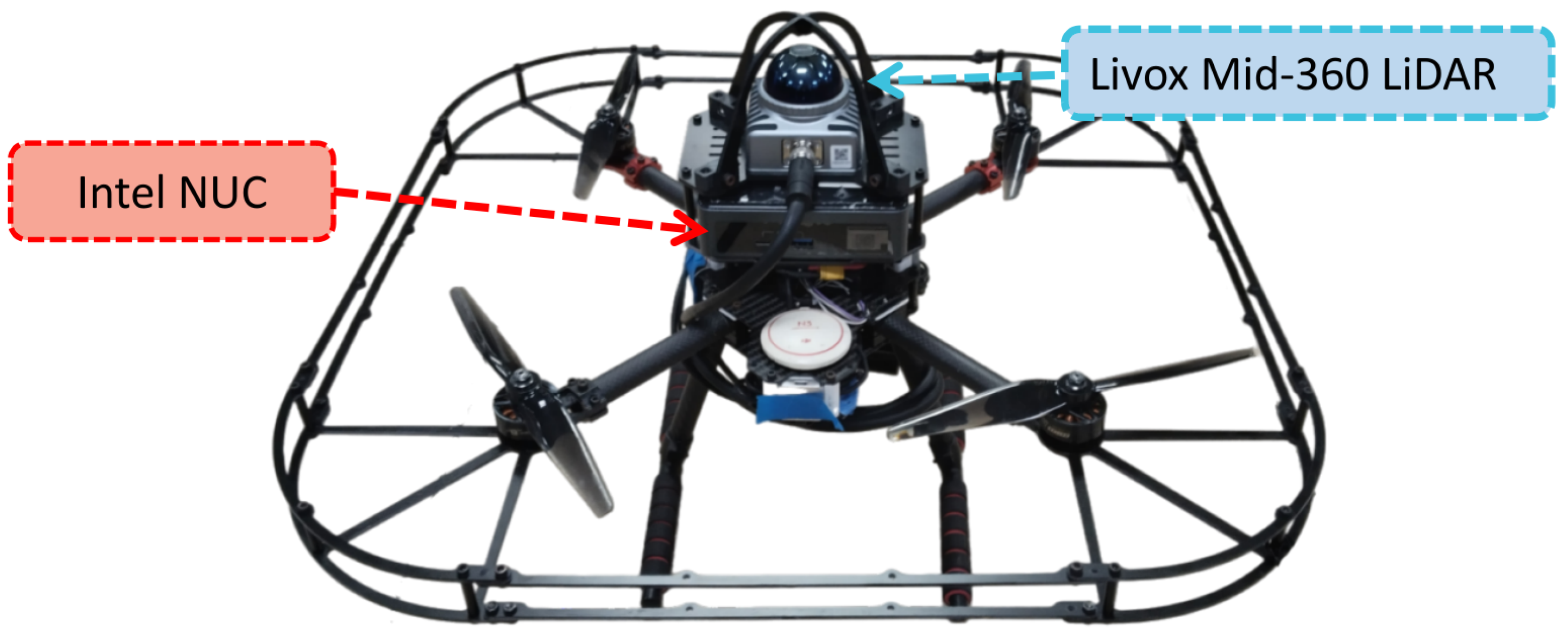
8. Real-World Experiments
9. Conclusions and Future Work
Author Contributions
Funding
Data Availability Statement
Conflicts of Interest
References
- Bircher, A.; Kamel, M.; Alexis, K.; Oleynikova, H.; Siegwart, R. Receding horizon path planning for 3D exploration and surface inspection. Auton. Robot. 2018, 42, 291–306. [Google Scholar] [CrossRef]
- Tabib, W.; Goel, K.; Yao, J.; Boirum, C.; Michael, N. Autonomous cave surveying with an aerial robot. IEEE Trans. Robot. 2021, 38, 1016–1032. [Google Scholar] [CrossRef]
- Wang, G.; Wang, W.; Ding, P.; Liu, Y.; Wang, H.; Fan, Z.; Bai, H.; Hongbiao, Z.; Du, Z. Development of a search and rescue robot system for the underground building environment. J. Field Robot. 2023, 40, 655–683. [Google Scholar] [CrossRef]
- Chatziparaschis, D.; Lagoudakis, M.G.; Partsinevelos, P. Aerial and Ground Robot Collaboration for Autonomous Mapping in Search and Rescue Missions. Drones 2020, 4, 79. [Google Scholar] [CrossRef]
- Han, D.; Jiang, H.; Wang, L.; Zhu, X.; Chen, Y.; Yu, Q. Collaborative Task Allocation and Optimization Solution for Unmanned Aerial Vehicles in Search and Rescue. Drones 2024, 8, 138. [Google Scholar] [CrossRef]
- Sharma, M.; Gupta, A.; Gupta, S.K. Mars Surface Exploration via Unmanned Aerial Vehicles: Secured MarSE UAV Prototype. In Holistic Approach to Quantum Cryptography in Cyber Security; CRC Press: Boca Raton, FL, USA, 2022; pp. 83–98. [Google Scholar]
- Yamauchi, B. A frontier-based approach for autonomous exploration. In Proceedings of the 1997 IEEE International Symposium on Computational Intelligence in Robotics and Automation CIRA’97.’Towards New Computational Principles for Robotics and Automation’, Monterey, CA, USA, 10–11 June 1997; pp. 146–151. [Google Scholar]
- González-Banos, H.H.; Latombe, J.C. Navigation strategies for exploring indoor environments. Int. J. Robot. Res. 2002, 21, 829–848. [Google Scholar] [CrossRef]
- Schmid, L.; Pantic, M.; Khanna, R.; Ott, L.; Siegwart, R.; Nieto, J. An efficient sampling-based method for online informative path planning in unknown environments. IEEE Robot. Autom. Lett. 2020, 5, 1500–1507. [Google Scholar] [CrossRef]
- Bircher, A.; Kamel, M.; Alexis, K.; Oleynikova, H.; Siegwart, R. Receding horizon ’next-best-view’ planner for 3d exploration. In Proceedings of the 2016 IEEE International Conference on Robotics and Automation (ICRA), Stockholm, Sweden, 16–21 May 2016; pp. 1462–1468. [Google Scholar]
- Dang, T.; Tranzatto, M.; Khattak, S.; Mascarich, F.; Alexis, K.; Hutter, M. Graph-based subterranean exploration path planning using aerial and legged robots. J. Field Robot. 2020, 37, 1363–1388. [Google Scholar] [CrossRef]
- Zhu, H.; Cao, C.; Xia, Y.; Scherer, S.; Zhang, J.; Wang, W. DSVP: Dual-stage viewpoint planner for rapid exploration by dynamic expansion. In Proceedings of the 2021 IEEE/RSJ International Conference on Intelligent Robots and Systems (IROS), Prague, Czech Republic, 27 September–1 October 2021; pp. 7623–7630. [Google Scholar]
- Kulich, M.; Faigl, J.; Přeučil, L. On distance utility in the exploration task. In Proceedings of the 2011 IEEE International Conference on Robotics and Automation (ICRA), Shanghai, China, 9–13 May 2011; pp. 4455–4460. [Google Scholar]
- Heng, L.; Gotovos, A.; Krause, A.; Pollefeys, M. Efficient visual exploration and coverage with a micro aerial vehicle in unknown environments. In Proceedings of the 2015 IEEE International Conference on Robotics and Automation (ICRA), Seattle, WA, USA, 26–30 May 2015; pp. 1071–1078. [Google Scholar]
- Faigl, J.; Kulich, M. On determination of goal candidates in frontier-based multi-robot exploration. In Proceedings of the 2013 European Conference on Mobile Robots, Catalonia, Spain, 25–27 September 2013; pp. 210–215. [Google Scholar]
- Cieslewski, T.; Kaufmann, E.; Scaramuzza, D. Rapid exploration with multi-rotors: A frontier selection method for high speed flight. In Proceedings of the 2017 IEEE/RSJ International Conference on Intelligent Robots and Systems (IROS), Vancouver, BC, Canada, 24–28 September 2017; pp. 2135–2142. [Google Scholar]
- Rekleitis, I.M.; Dujmovic, V.; Dudek, G. Efficient topological exploration. In Proceedings of the 1999 IEEE International Conference on Robotics and Automation (Cat. No. 99CH36288C), Detroit, MI, USA, 10–15 May 1999; Volume 1, pp. 676–681. [Google Scholar]
- Choset, H.; Walker, S.; Eiamsa-Ard, K.; Burdick, J. Sensor-based exploration: Incremental construction of the hierarchical generalized Voronoi graph. Int. J. Robot. Res. 2000, 19, 126–148. [Google Scholar] [CrossRef]
- Brass, P.; Cabrera-Mora, F.; Gasparri, A.; Xiao, J. Multirobot tree and graph exploration. IEEE Trans. Robot. 2011, 27, 707–717. [Google Scholar] [CrossRef]
- Akdeniz, B.C.; Bozma, H.I. Exploration and topological map building in unknown environments. In Proceedings of the 2015 IEEE International Conference on Robotics and Automation (ICRA), Seattle, WA, USA, 26–30 May 2015; pp. 1079–1084. [Google Scholar]
- Bourgault, F.; Makarenko, A.A.; Williams, S.B.; Grocholsky, B.; Durrant-Whyte, H.F. Information based adaptive robotic exploration. In Proceedings of the IEEE/RSJ international Conference on Intelligent Robots and Systems, Lausanne, Switzerland, 30 September–4 October 2002; Volume 1, pp. 540–545. [Google Scholar]
- Stachniss, C.; Grisetti, G.; Burgard, W. Information gain-based exploration using rao-blackwellized particle filters. In Proceedings of the Robotics: Science and Systems, Cambridge, MA, USA, 8–11 June 2005; Volume 2, pp. 65–72. [Google Scholar]
- Bai, S.; Wang, J.; Chen, F.; Englot, B. Information-theoretic exploration with Bayesian optimization. In Proceedings of the 2016 IEEE/RSJ International Conference on Intelligent Robots and Systems (IROS), Daejeon, Republic of Korea, 9–14 October 2016; pp. 1816–1822. [Google Scholar]
- Henderson, T.; Sze, V.; Karaman, S. An efficient and continuous approach to information-theoretic exploration. In Proceedings of the 2020 IEEE International Conference on Robotics and Automation (ICRA), Paris, France, 31 May–31 August 2020; pp. 8566–8572. [Google Scholar]
- Zhu, H.; Chung, J.J.; Lawrance, N.R.; Siegwart, R.; Alonso-Mora, J. Online informative path planning for active information gathering of a 3d surface. In Proceedings of the 2021 IEEE International Conference on Robotics and Automation (ICRA), Xian, China, 30 May–5 June 2021; pp. 1488–1494. [Google Scholar]
- LaValle, S.M. Rapidly-exploring random Trees: A new tool for path planning. In Research Report (TR 98-11); Computer Science Department, Iowa State University: Ames, IA, USA, 1998. [Google Scholar]
- Papachristos, C.; Khattak, S.; Alexis, K. Uncertainty-aware receding horizon exploration and mapping using aerial robots. In Proceedings of the 2017 IEEE international conference on robotics and automation (ICRA), Singapore, 29 May–3 June 2017; pp. 4568–4575. [Google Scholar]
- Witting, C.; Fehr, M.; Bähnemann, R.; Oleynikova, H.; Siegwart, R. History-aware autonomous exploration in confined environments using mavs. In Proceedings of the 2018 IEEE/RSJ International Conference on Intelligent Robots and Systems (IROS), Madrid, Spain, 1–5 October 2018; pp. 1–9. [Google Scholar]
- Dang, T.; Papachristos, C.; Alexis, K. Visual saliency-aware receding horizon autonomous exploration with application to aerial robotics. In Proceedings of the 2018 IEEE International Conference on Robotics and Automation (ICRA), Brisbane, Australia, 21–25 May 2018; pp. 2526–2533. [Google Scholar]
- Selin, M.; Tiger, M.; Duberg, D.; Heintz, F.; Jensfelt, P. Efficient autonomous exploration planning of large-scale 3d environments. IEEE Robot. Autom. Lett. 2019, 4, 1699–1706. [Google Scholar] [CrossRef]
- Zhou, B.; Zhang, Y.; Chen, X.; Shen, S. FUEL: Fast UAV exploration using incremental frontier structure and hierarchical planning. IEEE Robot. Autom. Lett. 2021, 6, 779–786. [Google Scholar] [CrossRef]
- Cao, C.; Zhu, H.; Choset, H.; Zhang, J. TARE: A Hierarchical Framework for Efficiently Exploring Complex 3D Environments. In Proceedings of the Robotics: Science and Systems, Virtually, 12–16 July 2021. [Google Scholar]
- Huang, J.; Zhou, B.; Fan, Z.; Zhu, Y.; Jie, Y.; Li, L.; Cheng, H. FAEL: Fast autonomous exploration for large-scale environments with a mobile robot. IEEE Robot. Autom. Lett. 2023, 8, 1667–1674. [Google Scholar] [CrossRef]
- Georgakis, G.; Bucher, B.; Arapin, A.; Schmeckpeper, K.; Matni, N.; Daniilidis, K. Uncertainty-driven planner for exploration and navigation. In Proceedings of the 2022 International Conference on Robotics and Automation (ICRA), Philadelphia, PA, USA, 23–27 May 2022; pp. 11295–11302. [Google Scholar]
- Yan, Z.; Yang, H.; Zha, H. Active neural mapping. In Proceedings of the IEEE/CVF International Conference on Computer Vision, Paris, France, 1–6 October 2023; pp. 10981–10992. [Google Scholar]
- Tao, Y.; Wu, Y.; Li, B.; Cladera, F.; Zhou, A.; Thakur, D.; Kumar, V. Seer: Safe efficient exploration for aerial robots using learning to predict information gain. In Proceedings of the 2023 IEEE International Conference on Robotics and Automation (ICRA), London, UK, 29 May–2 June 2023; pp. 1235–1241. [Google Scholar]
- Zhao, Y.; Zhang, J.; Zhang, C. Deep-learning based autonomous-exploration for UAV navigation. Knowl.-Based Syst. 2024, 297, 111925. [Google Scholar] [CrossRef]
- Hornung, A.; Wurm, K.M.; Bennewitz, M.; Stachniss, C.; Burgard, W. OctoMap: An efficient probabilistic 3D mapping framework based on octrees. Auton. Robot. 2013, 34, 189–206. [Google Scholar] [CrossRef]
- Oleynikova, H.; Taylor, Z.; Fehr, M.; Siegwart, R.; Nieto, J. Voxblox: Incremental 3d euclidean signed distance fields for on-board mav planning. In Proceedings of the 2017 IEEE/RSJ International Conference on Intelligent Robots and Systems (IROS), Vancouver, BC, Canada, 24 September 2017; pp. 1366–1373. [Google Scholar]
- Han, L.; Gao, F.; Zhou, B.; Shen, S. Fiesta: Fast incremental euclidean distance fields for online motion planning of aerial robots. In Proceedings of the 2019 IEEE/RSJ International Conference on Intelligent Robots and Systems (IROS), The Venetian Macao, Macau, 3–8 November 2019; pp. 4423–4430. [Google Scholar]
- Duberg, D.; Jensfelt, P. UFOMap: An efficient probabilistic 3D mapping framework that embraces the unknown. IEEE Robot. Autom. Lett. 2020, 5, 6411–6418. [Google Scholar] [CrossRef]
- Hojjatoleslami, S.; Kittler, J. Region growing: A new approach. IEEE Trans. Image Process. 1998, 7, 1079–1084. [Google Scholar] [CrossRef]
- Roberts, M.; Dey, D.; Truong, A.; Sinha, S.; Shah, S.; Kapoor, A.; Hanrahan, P.; Joshi, N. Submodular trajectory optimization for aerial 3d scanning. In Proceedings of the IEEE International Conference on Computer Vision, Venice, Italy, 22–29 October 2017; pp. 5324–5333. [Google Scholar]
- Applegate, D.L.; Bixby, R.E.; Chvátal, V.; Cook, W.J. The Traveling Salesman Problem: A Computational Study; Princeton University Press: Princeton, NJ, USA, 2007. [Google Scholar]
- Lin, S.; Kernighan, B.W. An effective heuristic algorithm for the traveling-salesman problem. Oper. Res. 1973, 21, 498–516. [Google Scholar] [CrossRef]
- Helsgaun, K. An effective implementation of the Lin–Kernighan traveling salesman heuristic. Eur. J. Oper. Res. 2000, 126, 106–130. [Google Scholar] [CrossRef]
- Zhou, X.; Wang, Z.; Ye, H.; Xu, C.; Gao, F. Ego-planner: An esdf-free gradient-based local planner for quadrotors. IEEE Robot. Autom. Lett. 2020, 6, 478–485. [Google Scholar] [CrossRef]
- Usenko, V.; Von Stumberg, L.; Pangercic, A.; Cremers, D. Real-time trajectory replanning for MAVs using uniform B-splines and a 3D circular buffer. In Proceedings of the 2017 IEEE/RSJ International Conference on Intelligent Robots and Systems (IROS), Vancouver, BC, Canada, 24–28 September 2017; pp. 215–222. [Google Scholar]
- Kong, F.; Liu, X.; Tang, B.; Lin, J.; Ren, Y.; Cai, Y.; Zhu, F.; Chen, N.; Zhang, F. MARSIM: A light-weight point-realistic simulator for LiDAR-based UAVs. IEEE Robot. Autom. Lett. 2023, 8, 2954–2961. [Google Scholar] [CrossRef]
- Xu, W.; Cai, Y.; He, D.; Lin, J.; Zhang, F. FAST-LIO2: Fast Direct LiDAR-Inertial Odometry. IEEE Trans. Robot. 2022, 38, 2053–2073. [Google Scholar] [CrossRef]


| Scene | Indoor | Mountain | Village | ||||||||||||||||
|---|---|---|---|---|---|---|---|---|---|---|---|---|---|---|---|---|---|---|---|
| Resolution r (m) | 0.1 | 0.3 | 0.5 | 0.1 | 0.3 | 0.5 | 0.1 | 0.3 | 0.5 | ||||||||||
| Sensing Range (m) | 5 | 9 | 12 | 5 | 9 | 12 | 5 | 9 | 12 | ||||||||||
| metric | total memory usage (MB) | average update time (ms) | total memory usage (MB) | average update time (ms) | total memory usage (MB) | average update time (ms) | total memory usage (MB) | average update time (ms) | total memory usage (MB) | average update time (ms) | total memory usage (MB) | average update time (ms) | total memory usage (MB) | average update time (ms) | total memory usage (MB) | average update time (ms) | total memory usage (MB) | average update time (ms) | |
| method | |||||||||||||||||||
| Octomap [38] | 1038.9 | 1238 | 18.7 | 107 | 5.0 | 58 | 824.8 | 1176 | 31.8 | 122 | 7.2 | 54 | 1353.8 | 1793 | 44.9 | 184 | 12.5 | 74 | |
| Voxblox [39] | 1021.7 | 345 | 69.1 | 143 | 20.8 | 124 | 857.4 | 344 | 105.1 | 160 | 25.2 | 119 | 1754.1 | 332 | 125.3 | 202 | 40.8 | 115 | |
| FIESTA [40] | 7695.0 | 261 | 480.9 | 49 | 120.2 | 8 | 7695.0 | 232 | 480.9 | 36 | 240.5 | 11 | 7695.0 | 97 | 961.9 | 38 | 240.5 | 8 | |
| UFOmap [41] | 344.0 | 51 | 24.6 | 20 | 5.5 | 14 | 353.9 | 47 | 30.9 | 27 | 8.0 | 15 | 448.2 | 53 | 41.8 | 32 | 12.5 | 14 | |
| FAOmap | 64.8 | 112 | 6.9 | 28 | 2.1 | 17 | 76.5 | 117 | 8.0 | 28 | 2.6 | 17 | 120.7 | 114 | 12.1 | 30 | 4.7 | 17 | |
| FAOmap | Global Planning | Local Planning | |||||||||||
|---|---|---|---|---|---|---|---|---|---|---|---|---|---|
| Frontier Clustering | Road Map Updating | Path Planning | Viewpoint Generation | Path Determining | |||||||||
| param | r | R | n | l | |||||||||
| value | 0.5 m | 10 | 5 | 8 m | 2 m | 6 | 6 m | 100 | 0.1 | 1.0 m | 3 | 3 | 10 |
| Scene & Bounding Box For Exploration & Observable Volume | Method | Planning Computation Time (ms) | Total Exploration Time (s) | Total Movement Distance (m) | Average Speed (m/s) | ||
|---|---|---|---|---|---|---|---|
| avg | std | avg | std | ||||
| Indoor | FUEL [31] | 42 | 384.2 | 18.6 | 561.9 | 24.4 | 1.463 |
| 105 m × 60 m × 8 m | TARE [32] | 694 | 336.7 | 46.0 | 728.1 | 98.4 | 2.162 |
| 47,084 m3 | proposed | 29 | 205.9 | 16.2 | 494.4 | 35.4 | 2.401 |
| Mountain | FUEL [31] | 74 | 412.9 | 44.6 | 579.9 | 67.1 | 1.404 |
| 100 m × 100 m × 8 m | TARE [32] | 656 | 312.7 | 56.3 | 685.3 | 122.0 | 2.192 |
| 56,341 m3 | proposed | 20 | 196.8 | 22.2 | 487.2 | 49.2 | 2.476 |
| Village | FUEL [31] | 139 | 726.8 | 57.9 | 996.7 | 70.8 | 1.371 |
| 150 m × 100 m × 8 m | TARE [32] | 749 | 659.2 | 105.6 | 1387.6 | 220.3 | 2.105 |
| 94,463 m3 | proposed | 24 | 383.9 | 29.5 | 923.2 | 69.9 | 2.405 |
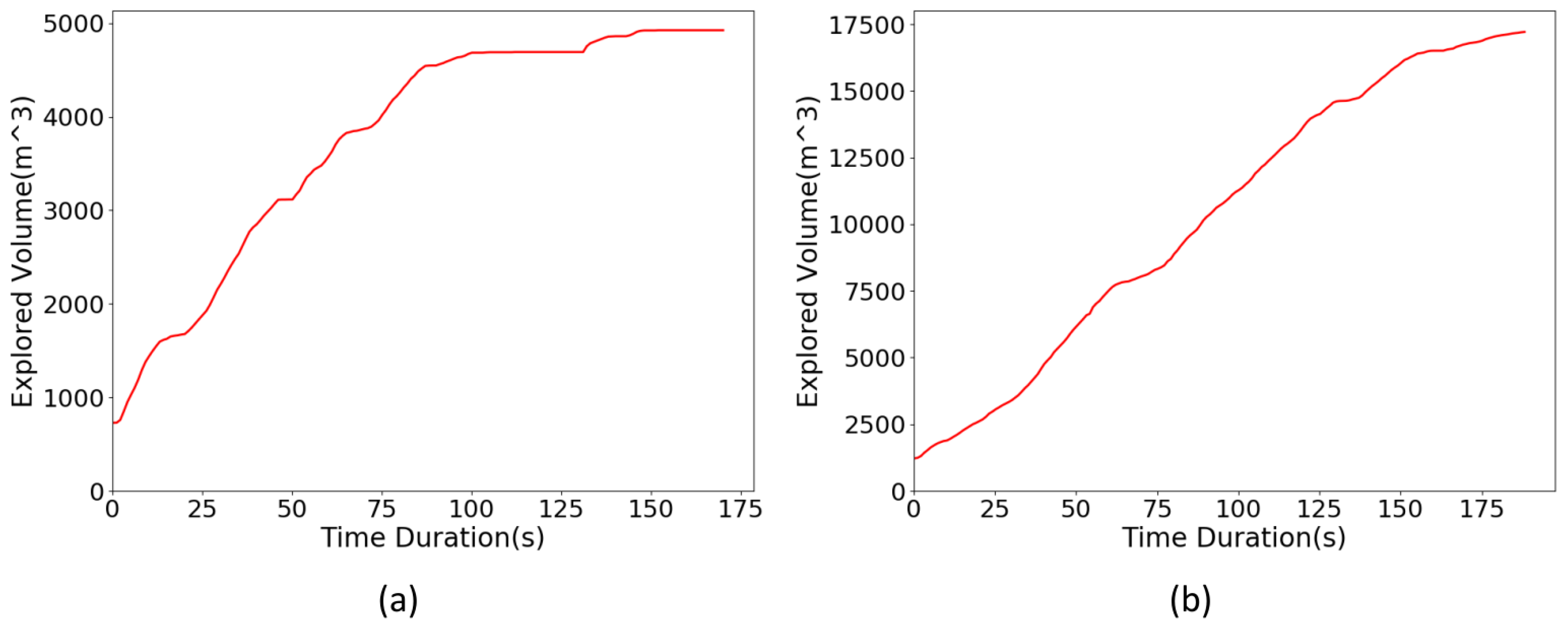
| Scene | Explored Time (s) | Movement Distance (m) | Explored Volume in Bounding Box (m3) | FAOmap Memory Usage (KB) | Average Planning Time (ms) |
|---|---|---|---|---|---|
| garage | 159 | 171 | 4924 | 173 | 19.7 |
| forest | 189 | 210 | 17,229 | 610 | 53.5 |
Disclaimer/Publisher’s Note: The statements, opinions and data contained in all publications are solely those of the individual author(s) and contributor(s) and not of MDPI and/or the editor(s). MDPI and/or the editor(s) disclaim responsibility for any injury to people or property resulting from any ideas, methods, instructions or products referred to in the content. |
© 2024 by the authors. Licensee MDPI, Basel, Switzerland. This article is an open access article distributed under the terms and conditions of the Creative Commons Attribution (CC BY) license (https://creativecommons.org/licenses/by/4.0/).
Share and Cite
Huang, J.; Fan, Z.; Yan, Z.; Duan, P.; Mei, R.; Cheng, H. Efficient UAV Exploration for Large-Scale 3D Environments Using Low-Memory Map. Drones 2024, 8, 443. https://doi.org/10.3390/drones8090443
Huang J, Fan Z, Yan Z, Duan P, Mei R, Cheng H. Efficient UAV Exploration for Large-Scale 3D Environments Using Low-Memory Map. Drones. 2024; 8(9):443. https://doi.org/10.3390/drones8090443
Chicago/Turabian StyleHuang, Junlong, Zhengping Fan, Zhewen Yan, Peiming Duan, Ruidong Mei, and Hui Cheng. 2024. "Efficient UAV Exploration for Large-Scale 3D Environments Using Low-Memory Map" Drones 8, no. 9: 443. https://doi.org/10.3390/drones8090443