


Monitoring Variability in Melt Pool Spatiotemporal Dynamics (VIMPS): Towards Proactive Humping Detection in Additive Manufacturing

Abstract
1. Introduction
- Transforms from reactive to proactive humping detection.
- Transforms humping detection from spatial (i.e., detachment) to spatiotemporal (i.e., elongation) abnormalities.
- Practically tracks the variability in solidification front dynamics.
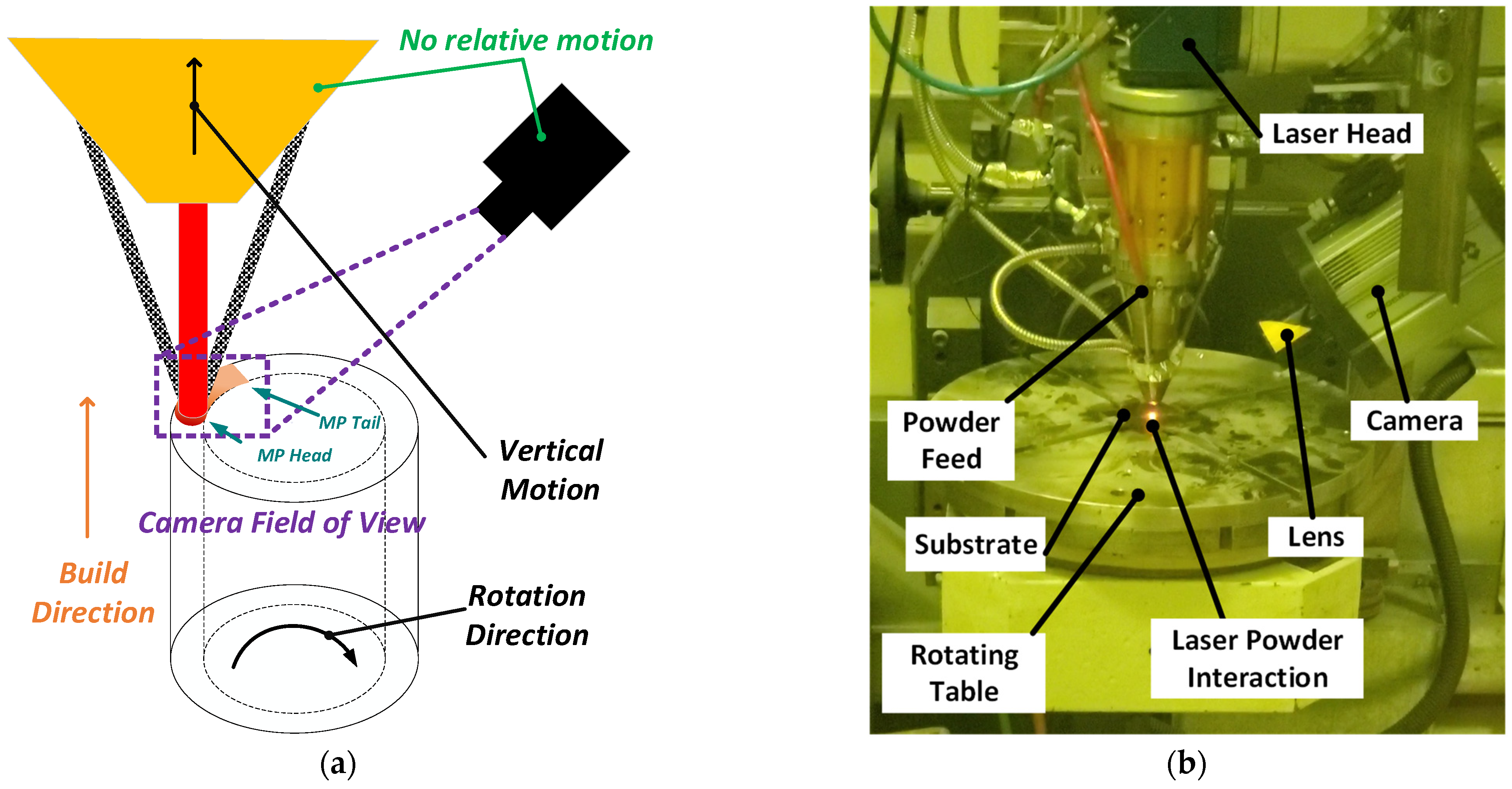
2. Experimental Setup
3. Signal Processing
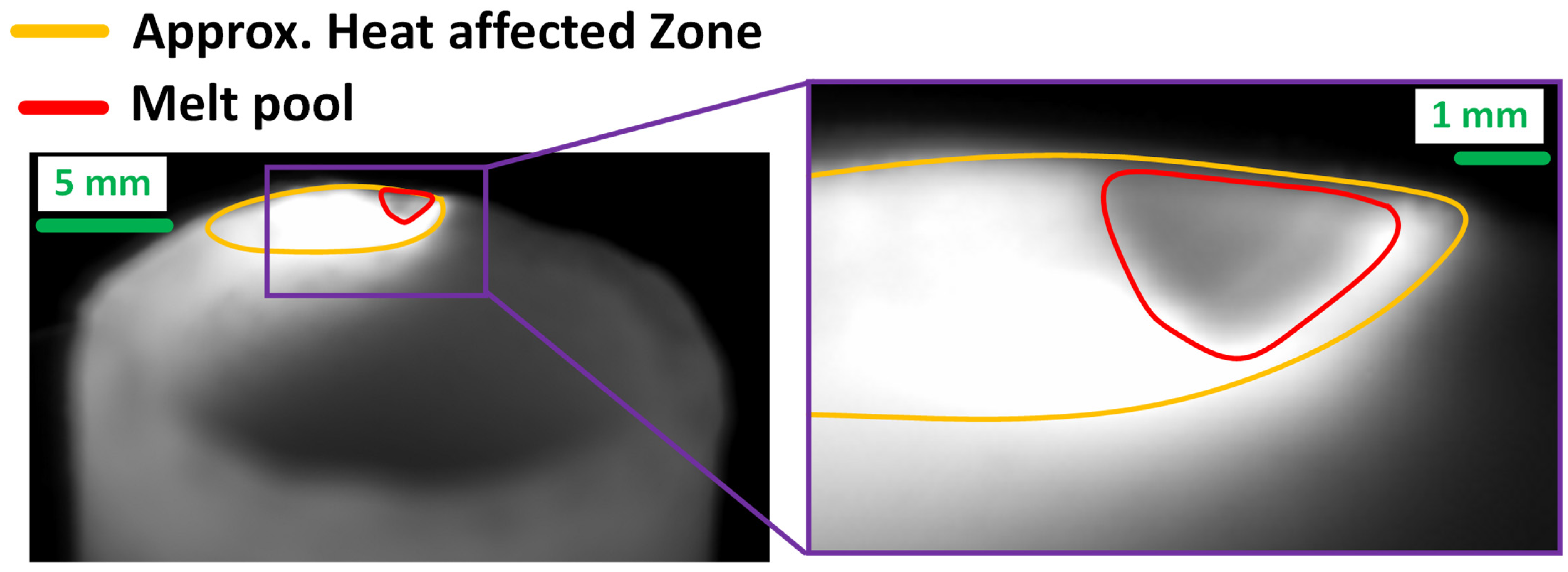
3.1. Pixel Intensity Physical Interpretation
3.2. Physics-Based Indicator
4. Results
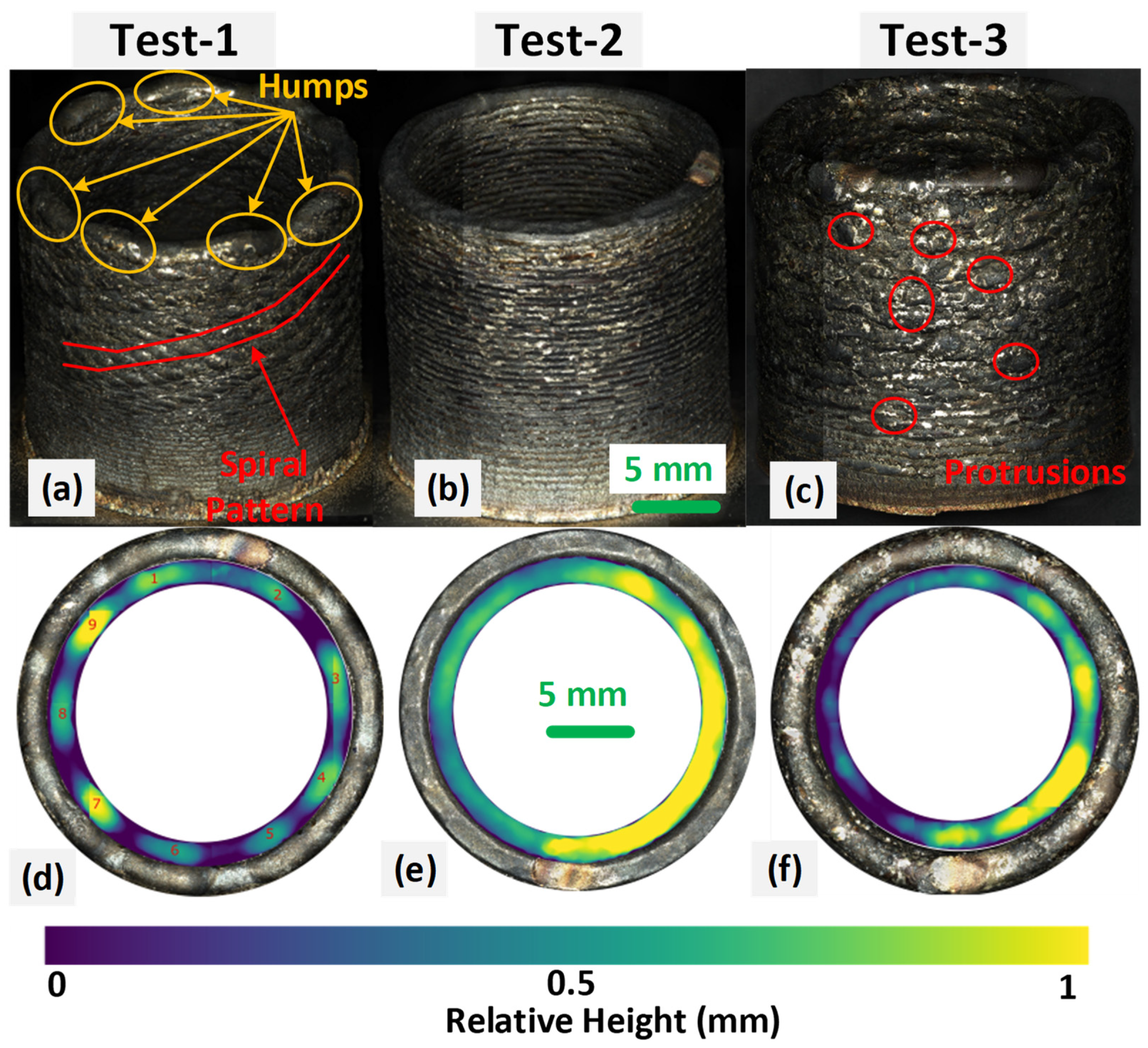
4.1. Geometrical Accuracy
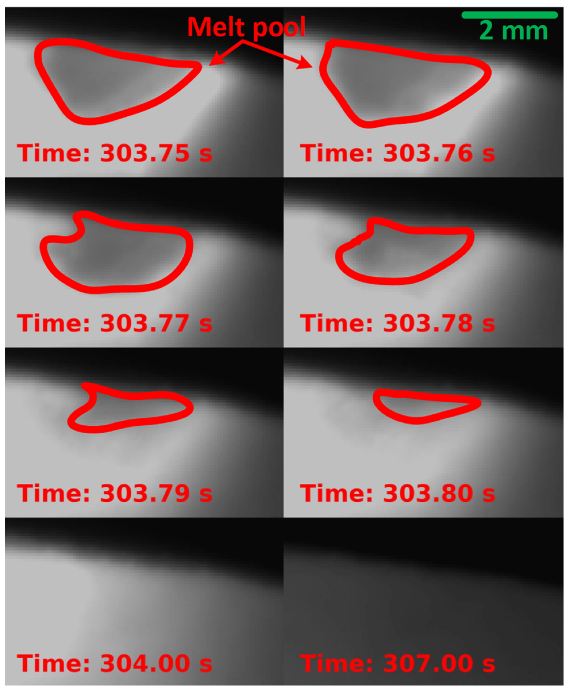
4.2. VIMPS Expressiveness of Geometrical Defects
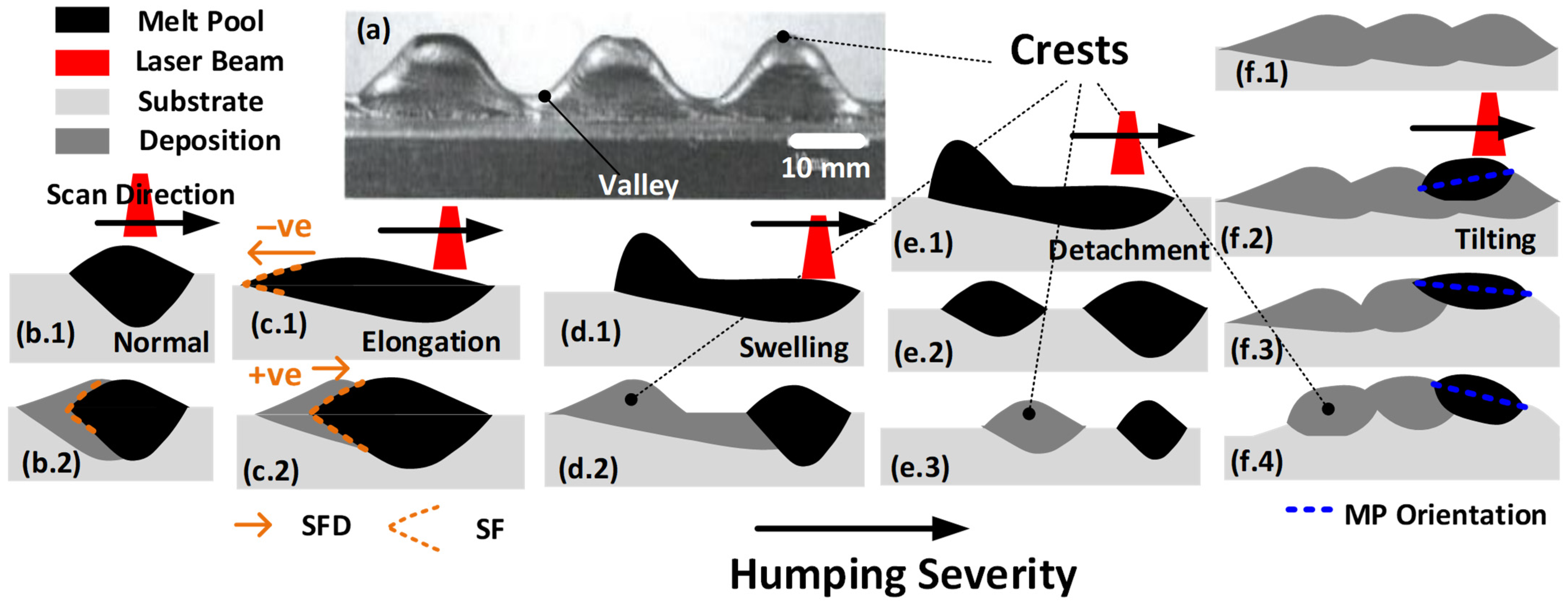
- It corrects the conceptual oversight related to the early stages of humping elongation modes.
- It acknowledges the temporal dynamics of humping, which are often overlooked.
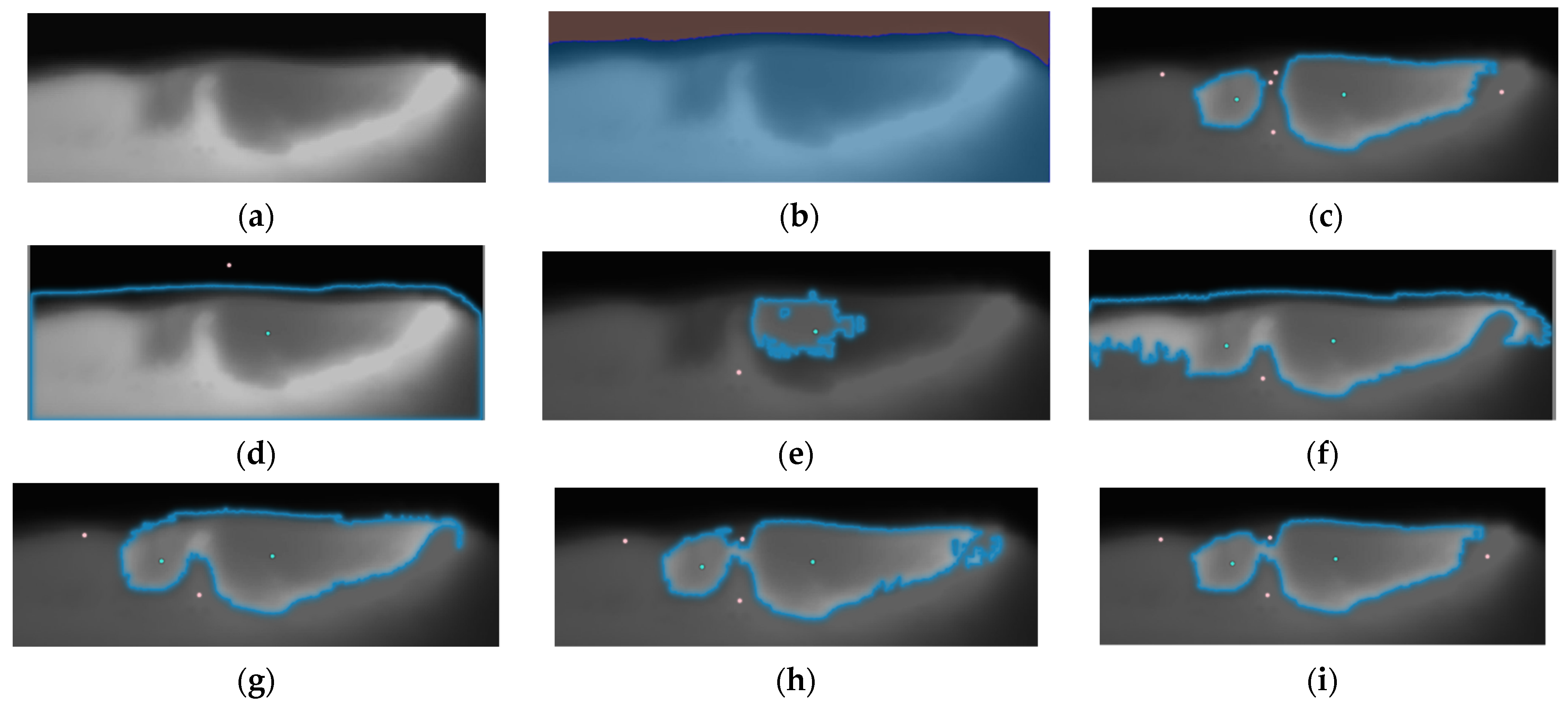
- It avoids the complexity of segmentation, reducing potential errors.
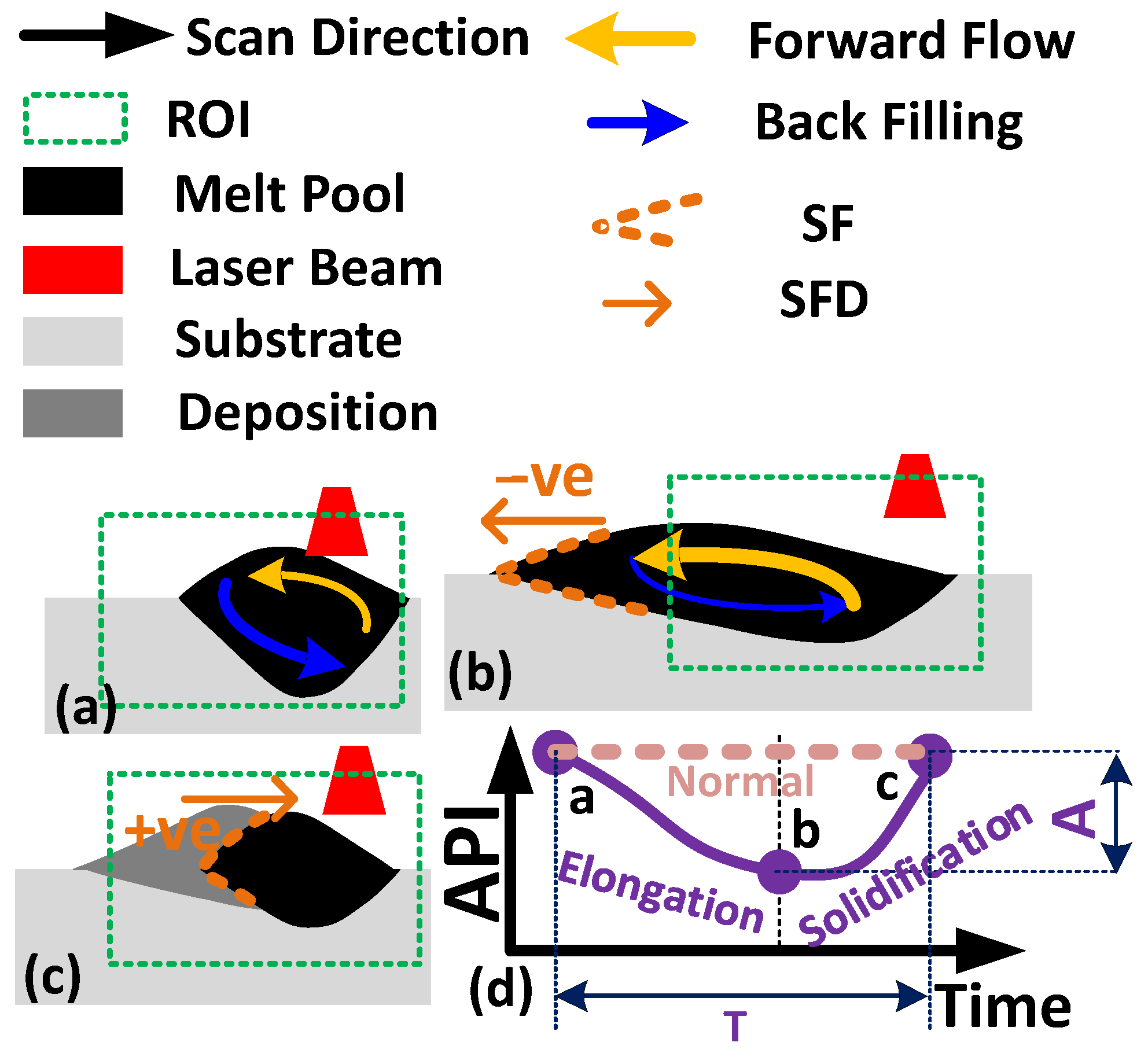
4.3. API Expressiveness of Solidification Spatiotemporal Dynamics
5. Conclusions
Supplementary Materials
Author Contributions
Funding
Data Availability Statement
Conflicts of Interest
Abbreviations
| A | The amplitude of the elongation cycle |
| API | Average pixel intensity |
| CDT | Continuous deposition time |
| DED | Direct energy deposition |
| DT | Dwell time |
| LE | Linear energy input |
| MP | Melt pool |
| SF | Solidification front |
| SFD | Solidification front relative velocity direction |
| T | Duration of the elongation cycle |
| VIMPS | Variability of instantaneous melt-pool solidification-front speed |
Appendix A
References
- Liu, Z.; He, B.; Lyu, T.; Zou, Y. A Review on Additive Manufacturing of Titanium Alloys for Aerospace Applications: Directed Energy Deposition and Beyond Ti-6Al-4V. JOM 2021, 73, 1804–1818. [Google Scholar] [CrossRef]
- Chen, H.; Liu, Z.; Cheng, X.; Zou, Y. Laser deposition of graded γ-TiAl/Ti2AlNb alloys: Microstructure and nanomechanical characterization of the transition zone. J. Alloys Compd. 2021, 875, 159946. [Google Scholar] [CrossRef]
- Ye, J.; Bab-hadiashar, A.; Alam, N.; Cole, I. A review of the parameter-signature-quality correlations through in situ sensing in laser metal additive manufacturing. Int. J. Adv. Manuf. Technol. 2023, 124, 1401–1427. [Google Scholar] [CrossRef]
- Yu, T.; Chen, L.; Liu, Z.; Xu, P. Research on the temperature control strategy of thin-wall parts fabricated by laser direct metal deposition. Int. J. Adv. Manuf. Technol. 2022, 122, 669–684. [Google Scholar] [CrossRef]
- Mianji, Z.; Kholopov, A.; Binkov, I.; Klimochkin, K. Experimental and Numerical Study of Heat Transfer in Thin-Walled Structures Built by Direct Metal Deposition and Geometry Improvement via Laser Power Modulation. Lasers Manuf. Mater. Process. 2023, 10, 353–372. [Google Scholar] [CrossRef]
- Svetlizky, D.; Das, M.; Zheng, B.; Vyatskikh, A.L.; Bose, S.; Bandyopadhyay, A.; Schoenung, J.M.; Lavernia, E.J.; Eliaz, N. Directed energy deposition (DED) additive manufacturing: Physical characteristics, defects, challenges and applications. Mater. Today 2021, 49, 271–295. [Google Scholar] [CrossRef]
- Tang, Z.J.; Liu, W.W.; Wang, Y.W.; Saleheen, K.M.; Liu, Z.C.; Peng, S.T.; Zhang, Z.; Zhang, H.C. A review on in situ monitoring technology for directed energy deposition of metals. Int. J. Adv. Manuf. Technol. 2020, 108, 3437–3463. [Google Scholar] [CrossRef]
- Adebayo, A.; Mehnen, J.; Tonnellier, X. Limiting Travel Speed in Additive Layer Manufacturing. In Proceedings of the 9th International Conference on Trends in Welding Research, Chicago, IL, USA, 4–8 June 2012. [Google Scholar]
- Turichin, G.; Zemlyakov, E.; Klimova, O.; Babkin, K. Hydrodynamic instability in high-speed direct laser deposition for additive manufacturing. Phys. Procedia 2016, 83, 674–683. [Google Scholar] [CrossRef]
- Nguyen, T.C.; Weckman, D.C.; Johnson, D.A.; Kerr, H.W. The humping phenomenon during high speed gas metal arc welding. Sci. Technol. Weld. Join. 2005, 10, 447–459. [Google Scholar] [CrossRef]
- Soderstrom, E.; Mendez, P. Humping mechanisms present in high speed welding. Sci. Technol. Weld. Join. 2006, 11, 572–579. [Google Scholar] [CrossRef]
- Zhang, M.; Liu, T.; Hu, R.; Mu, Z.; Chen, S.; Chen, G. Understanding root humping in high-power laser welding of stainless steels: A combination approach. Int. J. Adv. Manuf. Technol. 2020, 106, 5353–5364. [Google Scholar] [CrossRef]
- Yinglei, P.; Jiguo, S. Understanding humping formation based on keyhole and molten pool behaviour during high speed laser welding of thin sheets. Eng. Res. Express 2020, 2, 025031. [Google Scholar] [CrossRef]
- Ai, Y.; Jiang, P.; Wang, C.; Mi, G.; Geng, S.; Liu, W.; Han, C. Investigation of the humping formation in the high power and high speed laser welding. Opt. Lasers Eng. 2018, 107, 102–111. [Google Scholar] [CrossRef]
- Gullipalli, C.; Thawari, N.; Gupta, T.V.K. Humping defects in laser based direct metal deposition. Mater. Today Proc. 2023. [Google Scholar] [CrossRef]
- Shi, J.; Li, F.; Chen, S.; Zhao, Y.; Tian, H. Effect of in-process active cooling on forming quality and efficiency of tandem GMAW–based additive manufacturing. Int. J. Adv. Manuf. Technol. 2019, 101, 1349–1356. [Google Scholar] [CrossRef]
- Montevecchi, F.; Venturini, G.; Grossi, N.; Scippa, A.; Campatelli, G. Heat accumulation prevention in Wire-Arc-Additive-Manufacturing using air jet impingement. Manuf. Lett. 2018, 17, 14–18. [Google Scholar] [CrossRef]
- Montevecchi, F.; Venturini, G.; Grossi, N.; Scippa, A.; Campatelli, G. Idle time selection for wire-arc additive manufacturing: A finite element-based technique. Addit. Manuf. 2018, 21, 479–486. [Google Scholar] [CrossRef]
- Singh, S.; Jinoop, A.N.; Kumar, G.T.A.T.; Palani, I.A.; Paul, C.P.; Prashanth, K.G. Effect of interlayer delay on the microstructure and mechanical properties of wire arc additive manufactured wall structures. Materials 2021, 14, 4187. [Google Scholar] [CrossRef]
- Turgut, B.; Gürol, U.; Onler, R. Effect of interlayer dwell time on output quality in wire arc additive manufacturing of low carbon low alloy steel components. Int. J. Adv. Manuf. Technol. 2023, 126, 5277–5288. [Google Scholar] [CrossRef]
- Dababneh, F.; Taheri, H. Investigation of the influence of process interruption on mechanical properties of metal additive manufacturing parts. CIRP J. Manuf. Sci. Technol. 2022, 38, 706–716. [Google Scholar] [CrossRef]
- Denlinger, E.R.; Heigel, J.C.; Michaleris, P.; Palmer, T.A. Effect of inter-layer dwell time on distortion and residual stress in additive manufacturing of titanium and nickel alloys. J. Mater. Process. Technol. 2015, 215, 123–131. [Google Scholar] [CrossRef]
- Alfaro, S.C.A.; Vargas, J.A.R.; De Carvalho, G.C.; De Souza, G.G. Characterization of “humping” in the GTA welding process using infrared images. J. Mater. Process. Technol. 2015, 223, 216–224. [Google Scholar] [CrossRef]
- Xue, B.; Chang, B.; Du, D. A vision based method for humping detection in high-speed laser welding. J. Phys. Conf. Ser. 2021, 1983, 012074. [Google Scholar] [CrossRef]
- Lu, J.; Zhao, Z.; Han, J.; Bai, L. Hump weld bead monitoring based on transient temperature field of molten pool. Optik 2020, 208, 164031. [Google Scholar] [CrossRef]
- Altenburg, S.J.; Straße, A.; Gumenyuk, A.; Maierhofer, C. In-situ monitoring of a laser metal deposition (LMD) process: Comparison of MWIR, SWIR and high-speed NIR thermography. Quant. Infrared Thermogr. J. 2022, 19, 97–114. [Google Scholar] [CrossRef]
- Felice, R.A.; Nash, D.A. Pyrometry of materials with changing, spectrally-dependent emissivity-Solid and liquid metals. In Proceedings of the AIP Conference Proceedings, Los Angeles, CA, USA, 19–23 March 2012; Volume 1552, pp. 734–739. [Google Scholar] [CrossRef]
- Emissivity Values for Metals, (n.d.). Available online: https://www.flukeprocessinstruments.com/en-us/service-and-support/knowledge-center/infrared-technology/emissivity-metals (accessed on 4 October 2023).
- Slater, C.; Hechu, K.; Davis, C.; Sridhar, S. Characterisation of the solidification of a molten steel surface using infrared thermography. Metals 2019, 9, 126. [Google Scholar] [CrossRef]
- Kirillov, A.; Mintun, E.; Ravi, N.; Mao, H.; Rolland, C.; Gustafson, L.; Berg, A.; Lo, W.-Y.; Dollar, P.; Girshick, R. Segment Anything. 2023. Available online: https://ai.facebook.com/research/publications/segment-anything/ (accessed on 4 October 2023).
- Zhang, J.; Lyu, T.; Hua, Y.; Shen, Z.; Sun, Q.; Rong, Y.; Zou, Y. Image Segmentation for Defect Analysis in Laser Powder Bed Fusion: Deep Data Mining of X-Ray Photography from Recent Literature. Integr. Mater. Manuf. Innov. 2022, 11, 418–432. [Google Scholar] [CrossRef]
- Blumenstiel, B.; Jakubik, J.; Kühne, H.; Vössing, M. What a MESS: Multi-Domain Evaluation of Zero-Shot Semantic Segmentation. 2023. Available online: https://arxiv.org/abs/2306.15521v3 (accessed on 14 April 2024).
- Hassan, M.A.; ElMallah, R.; Lee, C.G. Approximate and Memorize (A&M): Settling opposing views in replay-based continuous unsupervised domain adaptation. Knowl.-Based Syst. 2024, 293, 111653. [Google Scholar] [CrossRef]
- Abubakr, M.; Akoush, B.; Khalil, A.; Hassan, M.A. Unleashing deep neural network full potential for solar radiation forecasting in a new geographic location with historical data scarcity: A transfer learning approach. Eur. Phys. J. Plus 2022, 137, 474. [Google Scholar] [CrossRef]
- Segment Anything|Meta AI, (n.d.). Available online: https://segment-anything.com/ (accessed on 14 April 2024).


| Test No. | P (W) | v (mm/min) |
|---|---|---|
| 1 | 650 | 600 |
| 2 | 650 | 360 |
| 3 | 850 | 360 |
| MP Size | SFD | API | |
|---|---|---|---|
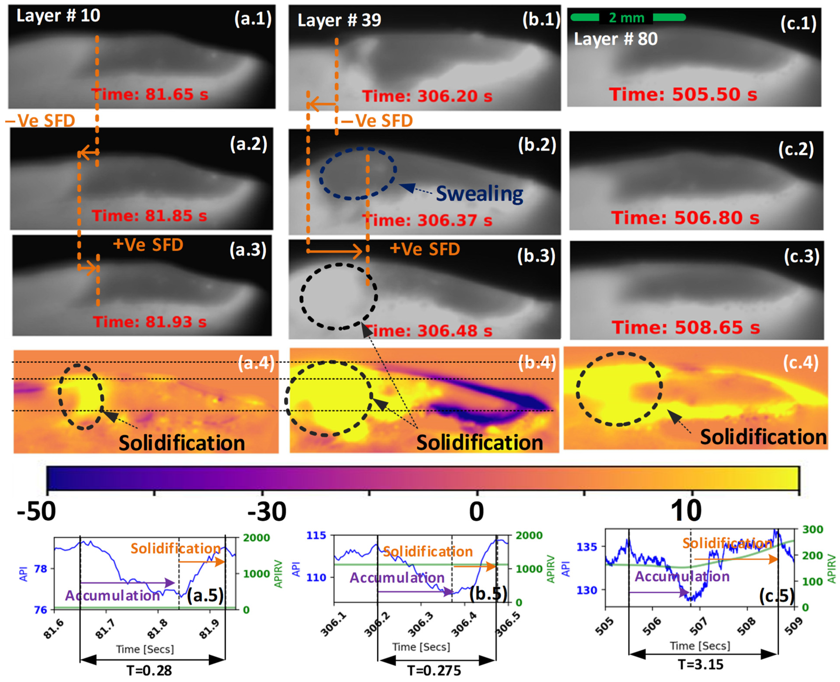
| Accumulation in Figure 1(c.1) | Increasing | Negative | Decreasing |
| Solidification in Figure 1(c.2) | Decreasing | Positive | Increasing |
| Line | Pseudo Code |
|---|---|
| 1 | Define Region of Interest (ROI) |
| 2 | For each time step do: |
| 3 | Calculate Average Pixel Intensity (API) as per Equation (1) |
| 4 | Calculate API’s Rolling Mean (APIRM) as per Equation (2) |
| 5 | Calculate API’s Rolling Variance (APIRV) as per Equation (3) |
| 6 | Calculate APIRVxM as per Equation (4) |
| 7 | Calculate (VIMPS) as per Equation (5) |
| 8 | End For |
| Metric | VIMPS | SOTA’s [24] Theoretical Upper Bound | ||
|---|---|---|---|---|
| Test # | 1 | 3 | 1 | 3 |
| Detection Time | 200 | 170 | 219 | 200 |
| T*Geo Time | 210 | 180 | 210 | 180 |
| Detection Lead | 10 | 10 | −9 | −20 |
| Consistency | High | Low | ||
| Complexity | Low | High | ||
| Principle | Spatiotemporal | Spatial | ||
| Mode | Elongation | Detachment | ||
Disclaimer/Publisher’s Note: The statements, opinions and data contained in all publications are solely those of the individual author(s) and contributor(s) and not of MDPI and/or the editor(s). MDPI and/or the editor(s) disclaim responsibility for any injury to people or property resulting from any ideas, methods, instructions or products referred to in the content. |
© 2024 by the authors. Licensee MDPI, Basel, Switzerland. This article is an open access article distributed under the terms and conditions of the Creative Commons Attribution (CC BY) license (https://creativecommons.org/licenses/by/4.0/).
Share and Cite
Hassan, M.A.; Hassan, M.; Lee, C.-G.; Sadek, A. Monitoring Variability in Melt Pool Spatiotemporal Dynamics (VIMPS): Towards Proactive Humping Detection in Additive Manufacturing. J. Manuf. Mater. Process. 2024, 8, 114. https://doi.org/10.3390/jmmp8030114
Hassan MA, Hassan M, Lee C-G, Sadek A. Monitoring Variability in Melt Pool Spatiotemporal Dynamics (VIMPS): Towards Proactive Humping Detection in Additive Manufacturing. Journal of Manufacturing and Materials Processing. 2024; 8(3):114. https://doi.org/10.3390/jmmp8030114
Chicago/Turabian StyleHassan, Mohamed Abubakr, Mahmoud Hassan, Chi-Guhn Lee, and Ahmad Sadek. 2024. "Monitoring Variability in Melt Pool Spatiotemporal Dynamics (VIMPS): Towards Proactive Humping Detection in Additive Manufacturing" Journal of Manufacturing and Materials Processing 8, no. 3: 114. https://doi.org/10.3390/jmmp8030114
APA StyleHassan, M. A., Hassan, M., Lee, C.-G., & Sadek, A. (2024). Monitoring Variability in Melt Pool Spatiotemporal Dynamics (VIMPS): Towards Proactive Humping Detection in Additive Manufacturing. Journal of Manufacturing and Materials Processing, 8(3), 114. https://doi.org/10.3390/jmmp8030114