
Manufacturing Process Optimization Using Open Data and Different Analysis Methods


Abstract
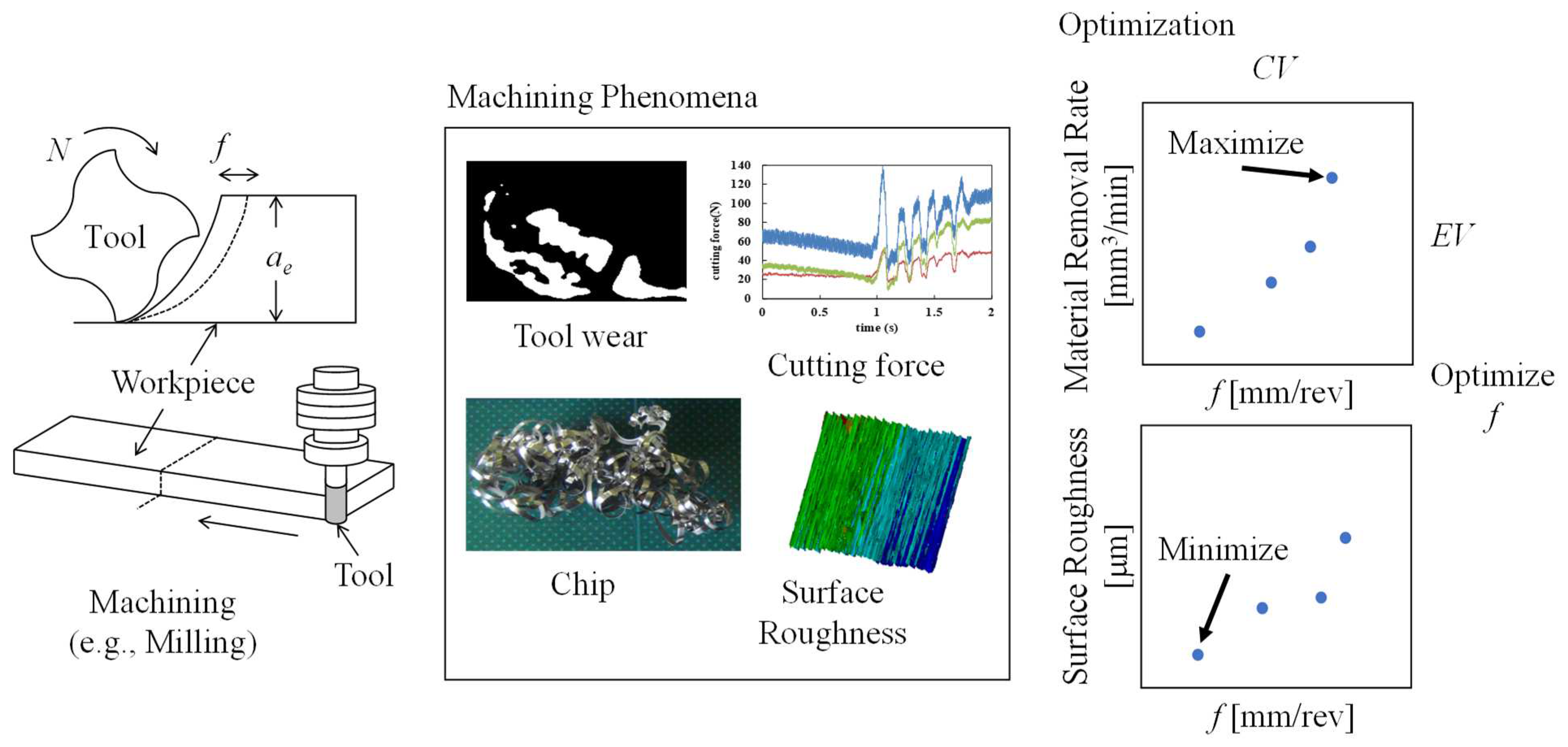
1. Introduction
2. Literature Review
2.1. Overview
2.2. Selected Studies
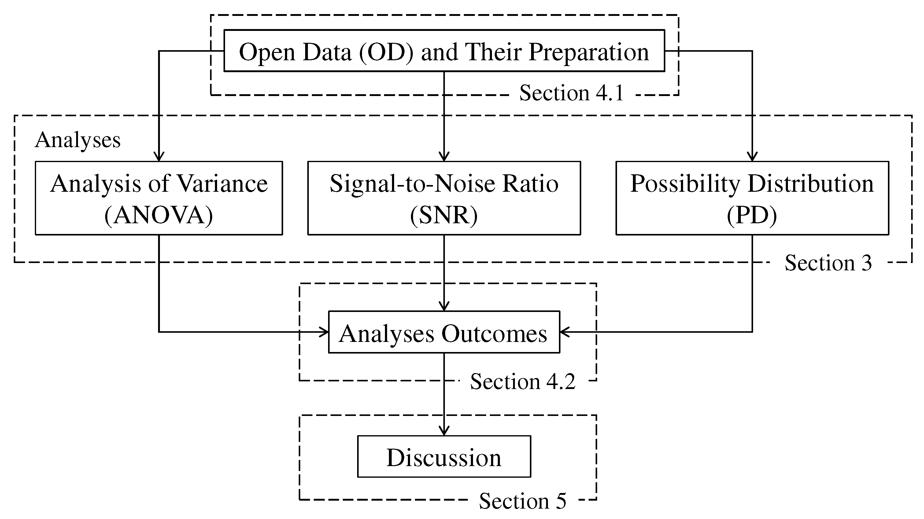
3. Methods
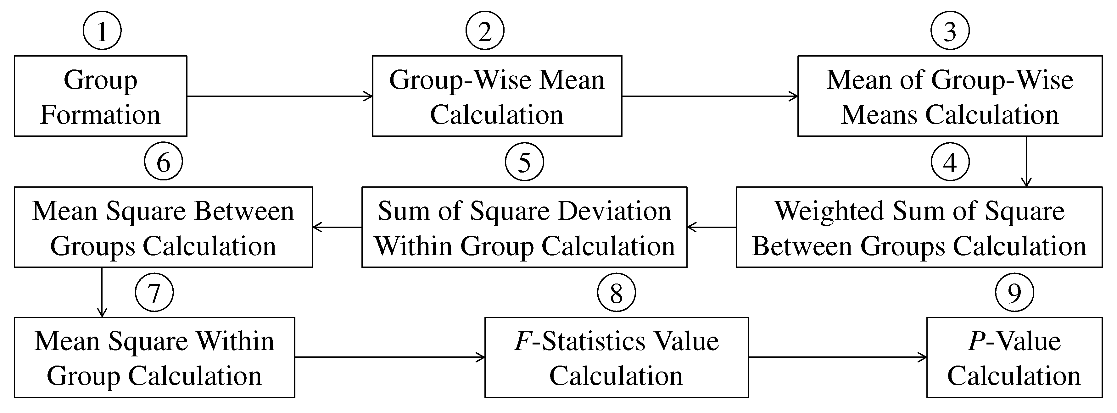
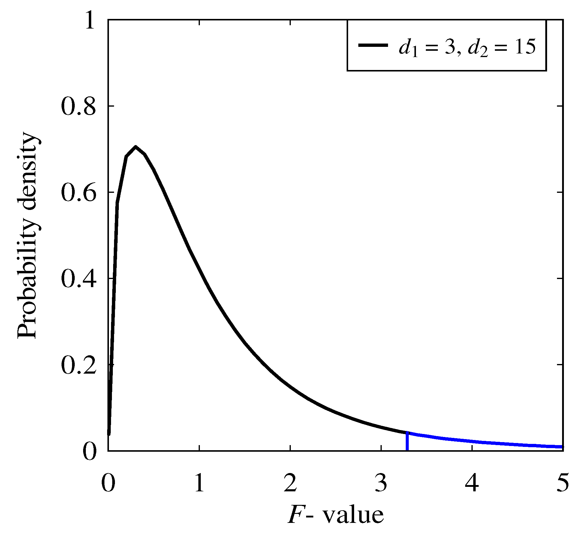
3.1. Analysis of Variance (ANOVA)
3.2. Signal-to-Noise Ratio (SNR)
3.2.1. Smaller-the-Better (STB)
3.2.2. Larger-the-Better (LTB)
3.2.3. Nominal-the-Better (NTB)
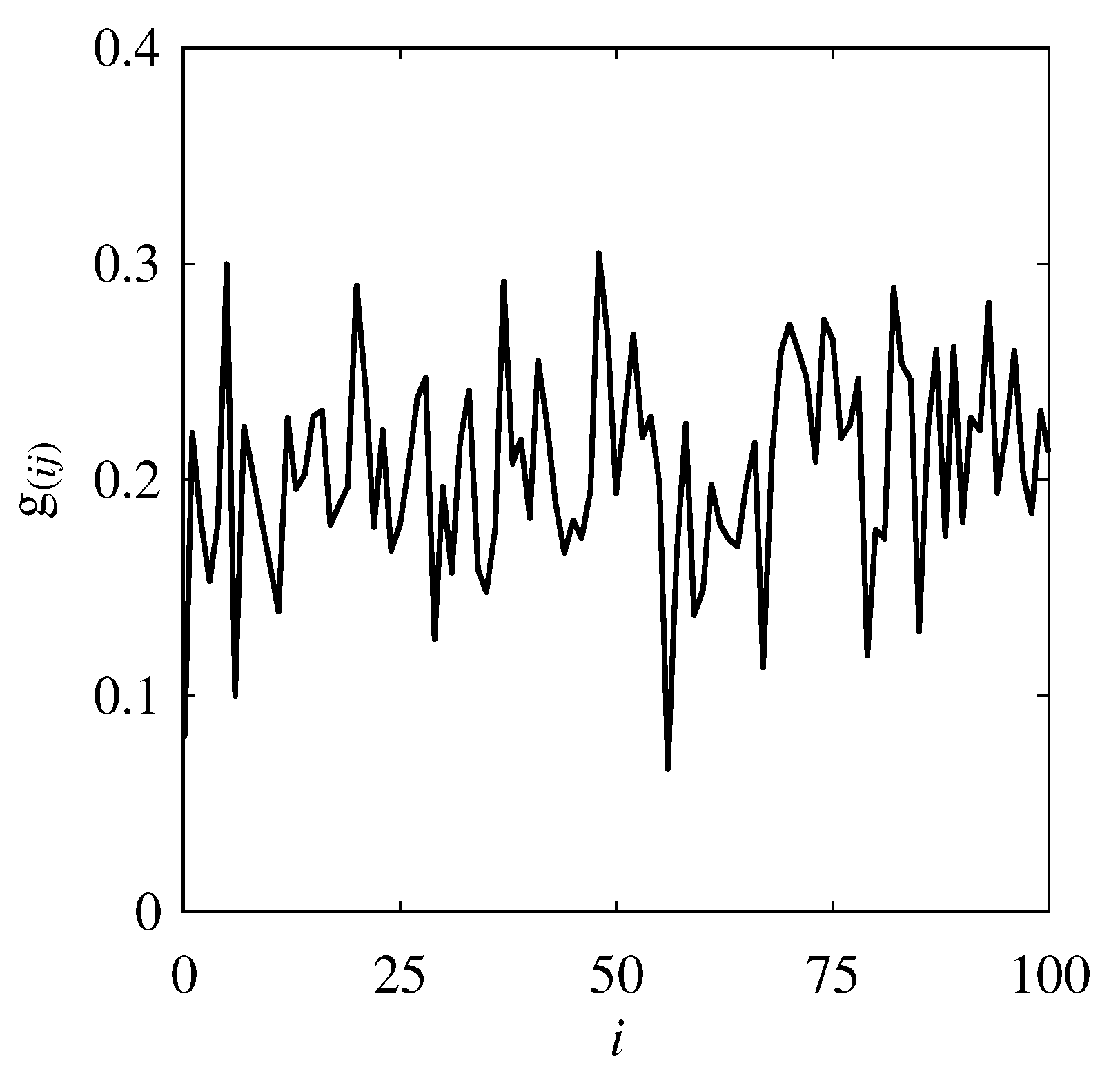
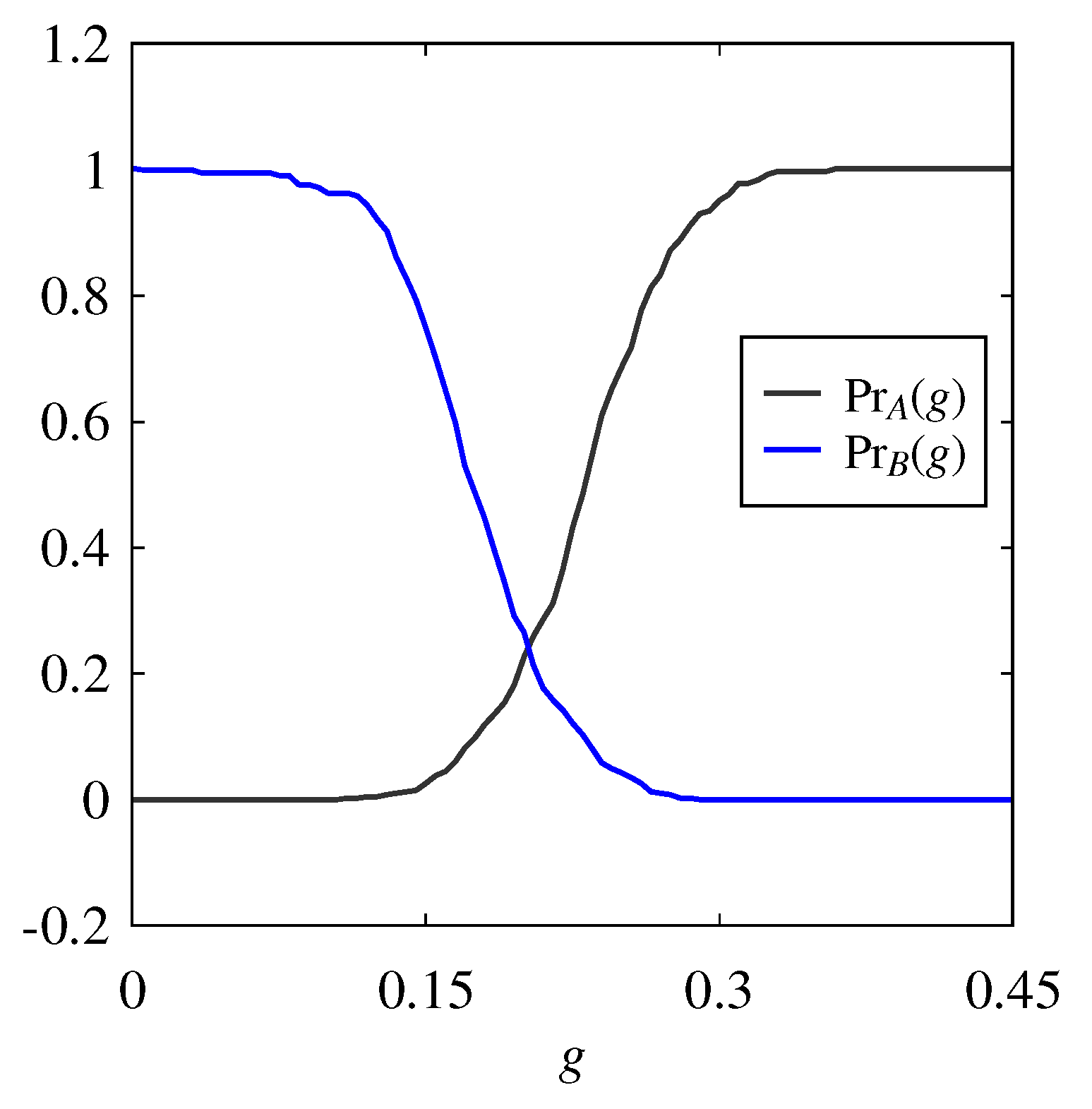
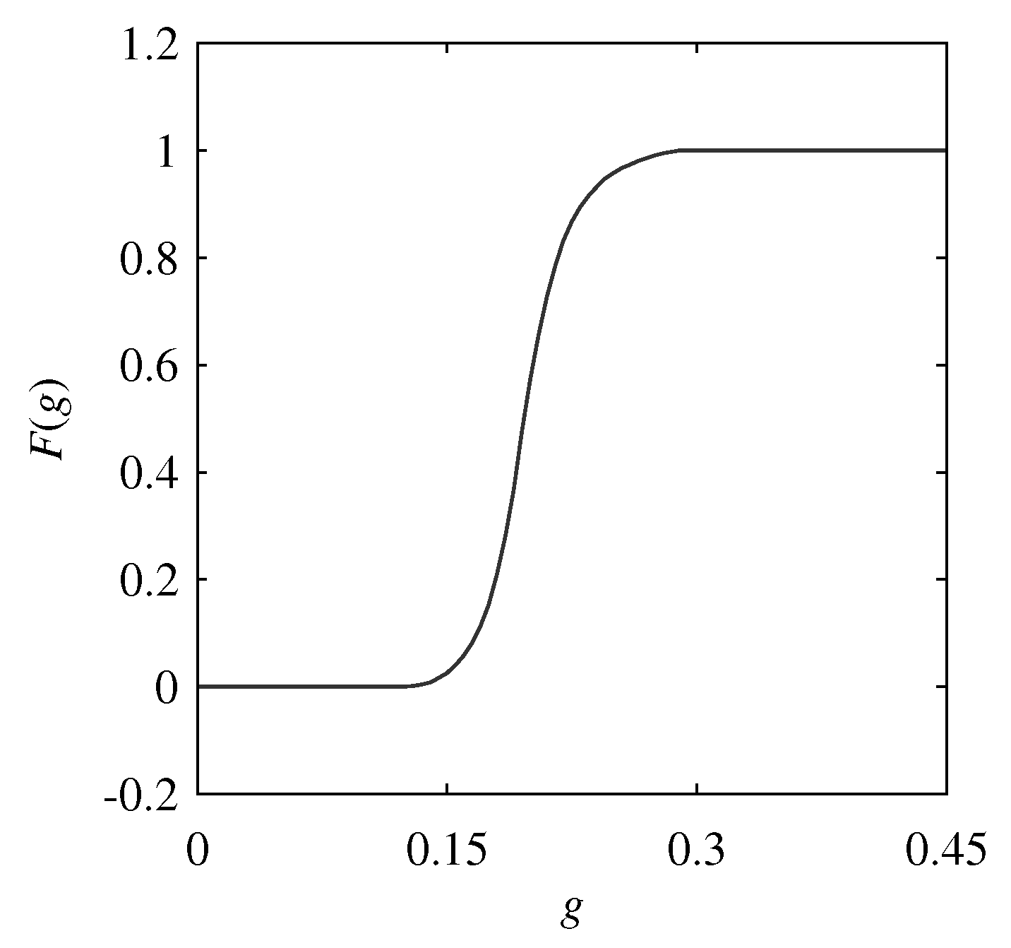
3.3. Possibility Distribution (PD)
4. Results
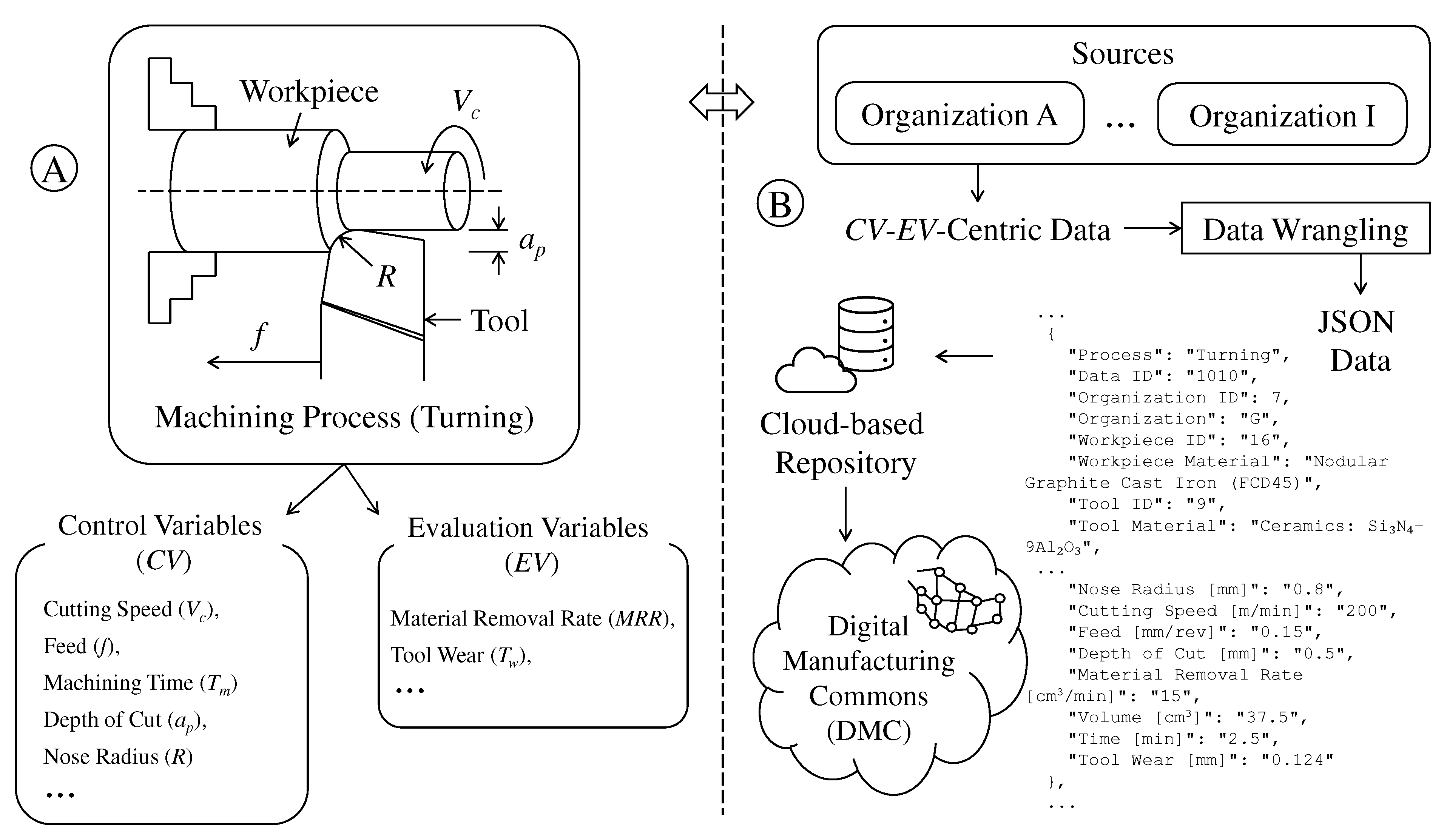
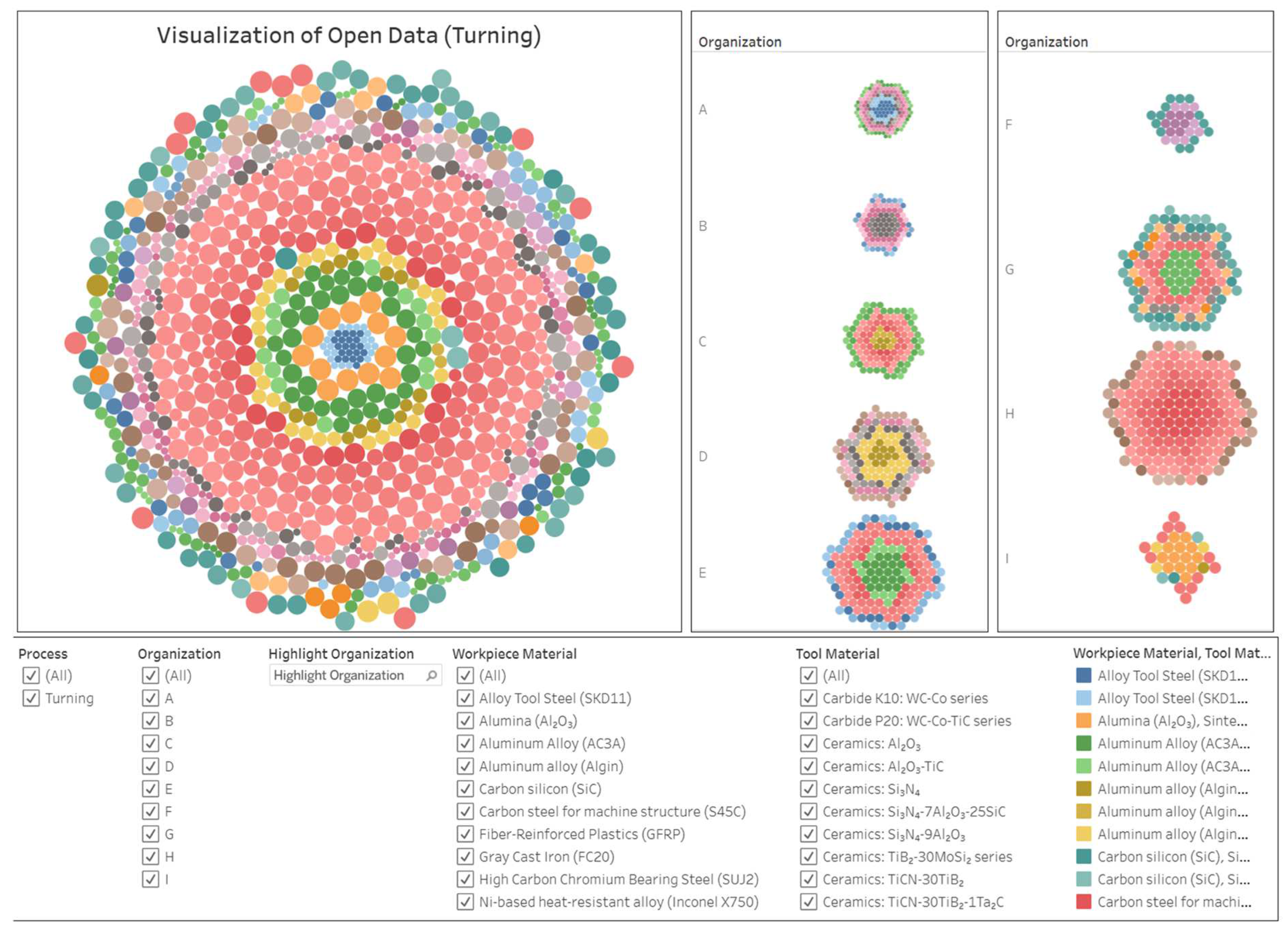
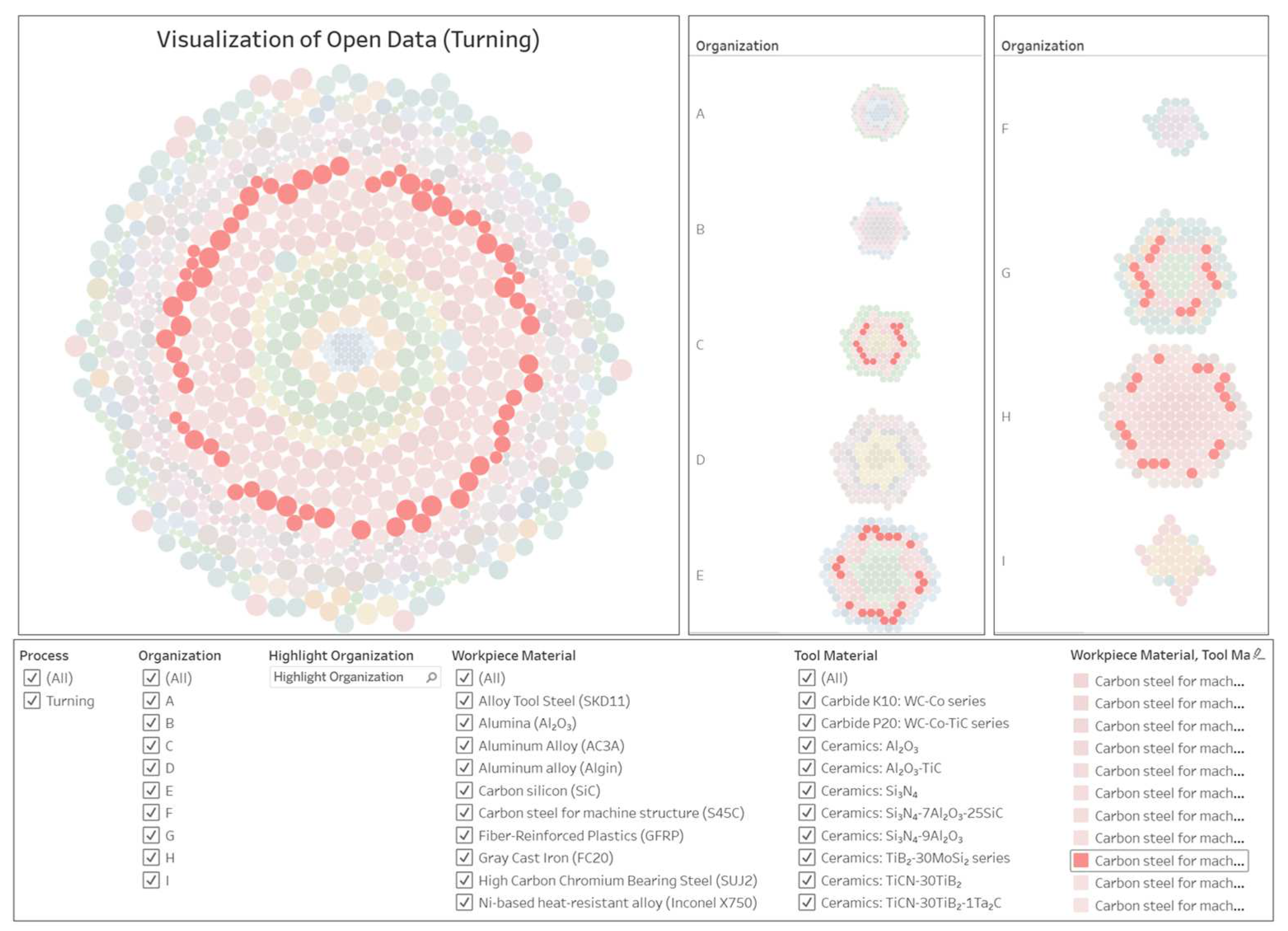
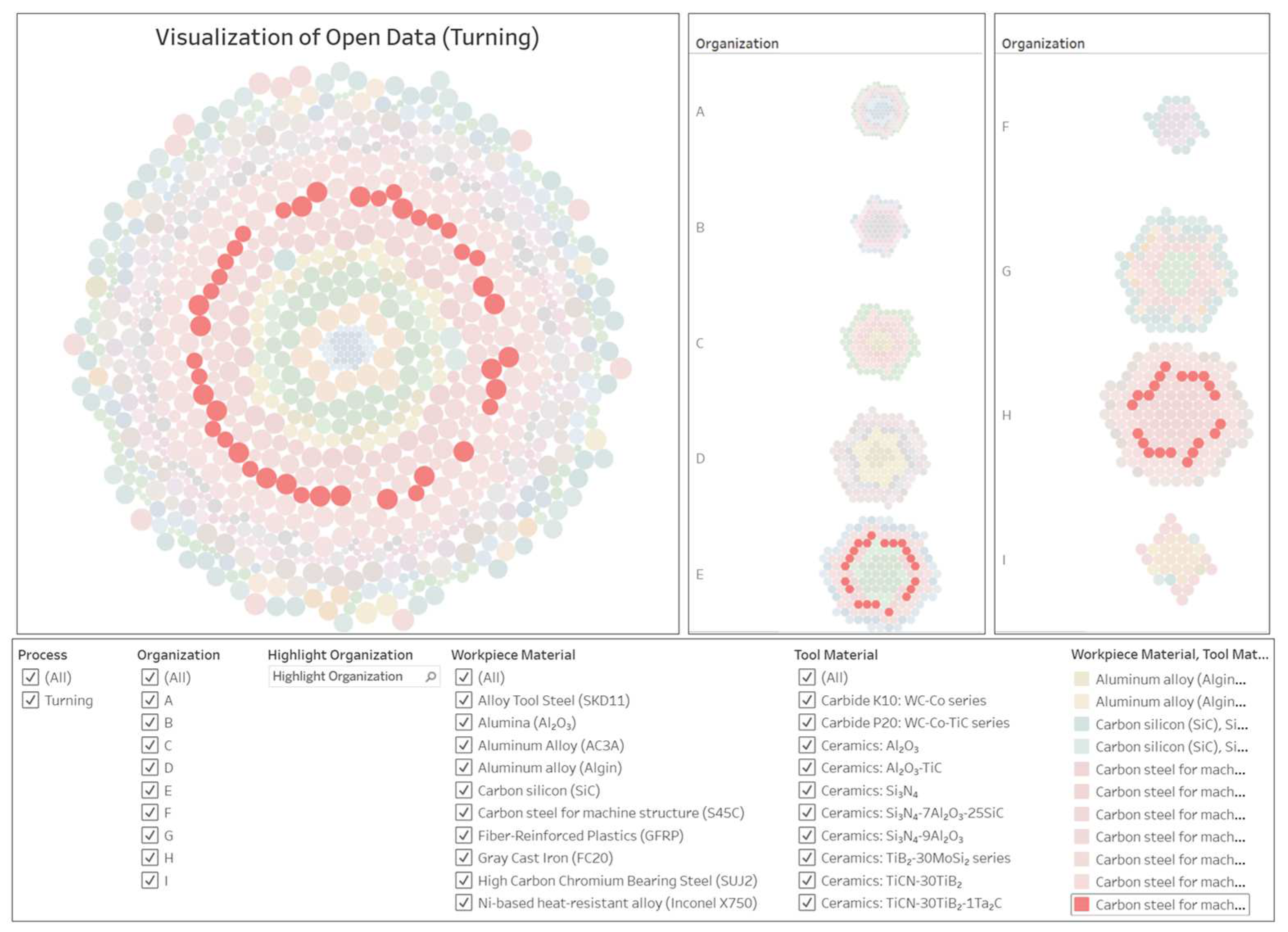
4.1. Open Data (OD) and Their Preparation
4.2. Analyses
4.2.1. WM1-TM1
4.2.2. WM1-TM2
5. Discussions
6. Conclusions
Author Contributions
Funding
Data Availability Statement
Acknowledgments
Conflicts of Interest
Appendix A. Section 2 (Literature Review)—Related Figures and Tables

| Method Type | Method | Purpose | Reference |
|---|---|---|---|
| Design of Experiments (DoE) |
| Creating structured CV-EV combinations for conducting experiments and data collection. | [10,11,14,19,20,21,22,23,24] |
| Statistical |
| Identifying significant CVs. | [10,11,12,13,14,15,16,20,25,26,27,28,33,35,36,37] |
| Identifying optimal CV states. | ||
| Developing predictive CV-EV relationships. | ||
| Determining optimal CVs for the experimental run. | ||
| Clustering |
| Interpreting complex CV-EV-centric datasets. | [29,30,31,32,33,34] |
| Machine Learning |
| Predictive modeling and real-time adaptation. | [10,19,25,38,39,40,41,42] |
| Metaheuristic Algorithms |
| Exploring optimal CVs from large CV-EV-centric datasets and multiple local optima. | [19,25,37,38,41,42] |
| Multi Objective Optimization |
| Evaluating multiple EVs together. | [37,43,44] |
| Adaptive Experimental Design |
| Reducing experimental runs adaptively based on prior results. | [19,45,46] |
| Fuzzy Reasoning |
| Handling uncertainty and imprecise CV-EV relationships and generating linguistics rules for decision making. | [5,17,18,47,48,49] |
| Reference | Process | Method | Optimization Criteria |
| [13] | CNC Turning |
| Determining optimal CVs (cutting speed, feed rate, and depth of cut) for maximizing the EV (material removal rate) and minimizing the EV (surface roughness). |
| [11] | CNC Turning |
| Determining optimal CVs (spindle speed, feed rate, and depth of cut) for maximizing the EV (material removal rate) and minimizing the EV (surface roughness). |
| [28] | Dry Turning |
| Determining optimal CVs (cutting speed, feed rate, and depth of cut) for maximizing the EV (material removal rate) and minimizing the EV (surface roughness). |
| [50] | Turning |
| Determining optimal CVs (cutting speed, feed rate, and air pressure) for minimizing the EVs (tool wear and surface roughness). |
| [38] | Wire Cut EDM |
| Determining optimal CVs (peak current, pulse on/off time, and wire feed rate) for maximizing the EV (material removal rate) and minimizing the EV (surface roughness). |
| [12] | Rotary Turning |
| Determining optimal CVs (cutting velocity, tool rotary speed, and feed rate) for minimizing the EVs (cutting force and surface roughness). |
| [15] | Turning |
| Determining optimal CVs (cutting velocity, feed, and depth of cut) for minimizing the EV (tool wear) and surface roughness while maximizing the EV (material removal rate). |
| [51] | Milling |
| Determining optimal CVs (spindle speed, feed, and axial/radial depth of cut) for maximizing cutting efficiency while minimizing the EVs (surface roughness and cutting force). |
| [36] | Grinding |
| Determining optimal CVs (feed velocity, depth of cut, and cooling/lubrication conditions) for minimizing the EVs (residual stress, surface roughness, production cost, and CO₂ emission) while maximizing the EVs (production rate and operator health). |
| [26] | Milling |
| Determining the optimal CVs (traverse speed, torch height, arc current, and gas pressure) for minimizing the EVs (kerf deviation and surface roughness) while maximizing the EV (micro hardness). |
| [25] | Milling |
| Determining the optimal CVs (cutting tool, feed rate, and spindle speed) for minimizing the EV (surface roughness). |
| [16] | End Milling |
| Determining optimal CVs (feed rate, cutting speed, and depth of cut) for minimizing the EV (surface roughness). |
| [37] | CNC Turning |
| Determining the optimal CVs for minimizing the EVs (surface roughness and cutting force). |
| [10] | Milling |
| Determining the optimal CVs (cutting speed, feed rate, depth of cut, and cooling/lubricating method) for minimizing the EV (surface roughness). |
| [35] | Turning |
| Determining optimal CVs (cutting speed, feed rate, and depth of cut) for maximizing the EV (material removal rate) while minimizing the EVs (surface roughness, cutting force, power consumption, heat rate, and peak tool temperature). |
| [19] | CNC End Milling |
| Determining optimal CVs (feed per tooth, cutting speed, and depth of cut) for maximizing the EV (material removal rate) while minimizing the EV (surface roughness). |
| [18] | Rotary Ultrasonic Machining |
| Analyzing the effects of CVs (ultrasonic power, feed rate, spindle speed, and tool diameter) on EVs (cutting force, tool wear, overcut error, and cylindricity error). |
| [20] | Dry Turning |
| Determining optimal CVs (cutting speed, feed rate, and depth of cut) for minimizing the EVs (surface roughness and cutting temperature). |
References
- Gupta, H.N. Manufacturing Process, 2nd ed.; New Age International Ltd.: New Delhi, India, 2009; ISBN 978-81-224-2844-5. [Google Scholar]
- Kalpakjian, S.; Schmid, S.R. Manufacturing Engineering and Technology; Eighth edition in SI Units; Pearson Education Limited: Harlow, UK, 2023; ISBN 978-1-292-42224-4. [Google Scholar]
- Tlusty, J. Manufacturing Processes and Equipment; Prentice Hall: Upper Saddle River, NJ, USA, 2000; ISBN 978-0-201-49865-3. [Google Scholar]
- Ullah, A.M.M.S. On the Interplay of Manufacturing Engineering Education and E-Learning. Int. J. Mech. Eng. Educ. 2016, 44, 233–254. [Google Scholar] [CrossRef]
- Ullah, A.M.M.S.; Harib, K.H. Manufacturing Process Performance Prediction by Integrating Crisp and Granular Information. J. Intell. Manuf. 2005, 16, 317–330. [Google Scholar] [CrossRef]
- Iwata, T.; Ghosh, A.K.; Ura, S. Toward Big Data Analytics for Smart Manufacturing: A Case of Machining Experiment. Proc. Int. Conf. Des. Concurr. Eng. Manuf. Syst. Conf. 2023, 2023, 33. [Google Scholar] [CrossRef]
- Ghosh, A.K.; Fattahi, S.; Ura, S. Towards Developing Big Data Analytics for Machining Decision-Making. J. Manuf. Mater. Process. 2023, 7, 159. [Google Scholar] [CrossRef]
- Kazuyuki, M. Survey of Big Data Use and Innovation in Japanese Manufacturing Firms (Online). 2025. Available online: https://www.rieti.go.jp/jp/publications/pdp/17p027.pdf (accessed on 19 February 2025).
- Beckmann, B.; Giani, A.; Carbone, J.; Koudal, P.; Salvo, J.; Barkley, J. Developing the Digital Manufacturing Commons: A National Initiative for US Manufacturing Innovation. Procedia Manuf. 2016, 5, 182–194. [Google Scholar] [CrossRef]
- Kosarac, A.; Tabakovic, S.; Mladjenovic, C.; Zeljkovic, M.; Orasanin, G. Next-Gen Manufacturing: Machine Learning for Surface Roughness Prediction in Ti-6Al-4V Biocompatible Alloy Machining. J. Manuf. Mater. Process. 2023, 7, 202. [Google Scholar] [CrossRef]
- Perumal, S.; Amarnath, M.K.; Marimuthu, K.; Subramaniam, P.; Rathinavelu, V.; Jagadeesh, D. Titanium Carbonitride–Coated CBN Insert Featured Turning Process Parameter Optimization during AA359 Alloy Machining. Int. J. Adv. Manuf. Technol. 2025, 136, 45–56. [Google Scholar] [CrossRef]
- Teimouri, R.; Amini, S.; Mohagheghian, N. Experimental Study and Empirical Analysis on Effect of Ultrasonic Vibration during Rotary Turning of Aluminum 7075 Aerospace Alloy. J. Manuf. Process. 2017, 26, 1–12. [Google Scholar] [CrossRef]
- Agarwal, S.; Suman, R.; Bahl, S.; Haleem, A.; Javaid, M.; Sharma, M.K.; Prakash, C.; Sehgal, S.; Singhal, P. Optimisation of Cutting Parameters during Turning of 16MnCr5 Steel Using Taguchi Technique. Int. J. Interact. Des. Manuf. IJIDeM 2024, 18, 2055–2066. [Google Scholar] [CrossRef]
- Chen, L.; Li, J.; Ma, Z.; Jiang, C.; Yu, T.; Gu, R. Grinding Performance and Parameter Optimization of Laser DED TiC Reinforced Ni-Based Composite Coatings. J. Manuf. Process. 2025, 134, 466–481. [Google Scholar] [CrossRef]
- Banerjee, A.; Maity, K. Hybrid Optimization Strategies for Improved Machinability of Nitronic-50 with MT-PVD Inserts. J. Manuf. Process. 2025, 137, 221–251. [Google Scholar] [CrossRef]
- Kechagias, J. Multiparameter Signal-to-Noise Ratio Optimization for End Milling Cutting Conditions of Aluminium Alloy 5083. Int. J. Adv. Manuf. Technol. 2024, 132, 4979–4988. [Google Scholar] [CrossRef]
- Fattahi, S.; Ullah, A.S. Optimization of Dry Electrical Discharge Machining of Stainless Steel Using Big Data Analytics. Procedia CIRP 2022, 112, 316–321. [Google Scholar] [CrossRef]
- Chowdhury, M.A.K.; Ullah, A.M.M.S.; Anwar, S. Drilling High Precision Holes in Ti6Al4V Using Rotary Ultrasonic Machining and Uncertainties Underlying Cutting Force, Toolwear, and Production Inaccuracies. Materials 2017, 10, 1069. [Google Scholar] [CrossRef]
- Mongan, P.G.; Hinchy, E.P.; O’Dowd, N.P.; McCarthy, C.T.; Diaz-Elsayed, N. An Ensemble Neural Network for Optimising a CNC Milling Process. J. Manuf. Syst. 2023, 71, 377–389. [Google Scholar] [CrossRef]
- Bouhali, R.; Bendjeffal, H.; Chetioui, K.B.; Bousba, I. Multivariable Optimization Based on the Taguchi Method to Study the Cutting Conditions in Aluminum Turning. Int. J. Interact. Des. Manuf. IJIDeM 2024. [Google Scholar] [CrossRef]
- Usgaonkar, G.G.S.; Gaonkar, R.S.P. GRA and CoCoSo Based Analysis for Optimal Performance Decisions in Sustainable Grinding Operation. Int. J. Math. Eng. Manag. Sci. 2025, 10, 1–21. [Google Scholar] [CrossRef]
- Ranganathan, R.; Saiyathibrahim, A.; Velu, R.; Jatti, V.S.; Mohan, D.G.; Vijayakumar, P. Achieving Multi-Response Optimization of Control Parameters for Wire-EDM on Additive Manufactured AlSi10Mg Alloy Using Taguchi-Grey Relational Theory. Eng. Res. Express 2025, 7, 015404. [Google Scholar] [CrossRef]
- Agarwal, D.; Yadav, S.; Singh, R.K.; Sharma, A.K. To Investigate the Effect of Discharge Energy and Addition of Nano-Powder on Processing of Micro Slots Using EDM Assisted µ-Milling Operation. Mater. Manuf. Process. 2025, 40, 80–94. [Google Scholar] [CrossRef]
- Fan, L.; Yang, G.; Zhang, Y.; Gao, L.; Wu, B. A Novel Tolerance Optimization Approach for Compressor Blades: Incorporating the Measured out-of-Tolerance Error Data and Aerodynamic Performance. Aerosp. Sci. Technol. 2025, 158, 109920. [Google Scholar] [CrossRef]
- Boga, C.; Koroglu, T. Proper Estimation of Surface Roughness Using Hybrid Intelligence Based on Artificial Neural Network and Genetic Algorithm. J. Manuf. Process. 2021, 70, 560–569. [Google Scholar] [CrossRef]
- Karthick, M.; Anand, P.; Siva Kumar, M.; Meikandan, M. Exploration of MFOA in PAC Parameters on Machining Inconel 718. Mater. Manuf. Process. 2022, 37, 1433–1445. [Google Scholar] [CrossRef]
- Kantheti, P.R.; Meena, K.L.; Chekuri, R.B.R. Maximizing Machining Efficiency and Quality in AA7075/Gr/B4 C HMMCs through Advanced DS-EDM Parameter Optimization Strategies. Eng. Res. Express 2024, 6, 045504. [Google Scholar] [CrossRef]
- Gangwar, S.; Mondal, S.C.; Kumar, A.; Ghadai, R.K. Performance Analysis and Optimization of Machining Parameters Using Coated Tungsten Carbide Cutting Tool Developed by Novel S3P Coating Method. Int. J. Interact. Des. Manuf. IJIDeM 2024, 18, 3909–3922. [Google Scholar] [CrossRef]
- Wan, L.; Chen, Z.; Zhang, X.; Wen, D.; Ran, X. A Multi-Sensor Monitoring Methodology for Grinding Wheel Wear Evaluation Based on INFO-SVM. Mech. Syst. Signal Process. 2024, 208, 111003. [Google Scholar] [CrossRef]
- Fu, X.; Li, K.; Zheng, M.; Wang, C.; Chen, E. Research on Dynamic Characteristics of Turning Process System Based on Finite Element Generalized Dynamics Space. Int. J. Adv. Manuf. Technol. 2024, 131, 4683–4698. [Google Scholar] [CrossRef]
- Cai, M.; Chen, M.; Gong, Y.; Gong, Q.; Zhu, T.; Zhang, M. Optimizing Grinding Parameters for Surface Integrity in Single Crystal Nickel Superalloys Using SVM Modeling. Int. J. Adv. Manuf. Technol. 2024, 135, 315–335. [Google Scholar] [CrossRef]
- Mohanta, D.K.; Sahoo, B.; Mohanty, A.M. Experimental Analysis for Optimization of Process Parameters in Machining Using Coated Tools. J. Eng. Appl. Sci. 2024, 71, 38. [Google Scholar] [CrossRef]
- Pathapalli, V.R.; Pittam, S.R.; Sarila, V.; Burragalla, D.; Gagandeep, A. Multi-Objective Parametric Optimization of AWJM Process Using Taguchi-Based GRA and DEAR Methodology. Proc. Inst. Mech. Eng. Part E J. Process Mech. Eng. 2024, 238, 2845–2853. [Google Scholar] [CrossRef]
- Chan, T.-C.; Wu, S.-C.; Ullah, A.; Farooq, U.; Wang, I.-H.; Chang, S.-L. Integrating Numerical Techniques and Predictive Diagnosis for Precision Enhancement in Roller Cam Rotary Table. Int. J. Adv. Manuf. Technol. 2024, 132, 3427–3445. [Google Scholar] [CrossRef]
- Tanvir, M.H.; Hussain, A.; Rahman, M.M.T.; Ishraq, S.; Zishan, K.; Rahul, S.T.T.; Habib, M.A. Multi-Objective Optimization of Turning Operation of Stainless Steel Using a Hybrid Whale Optimization Algorithm. J. Manuf. Mater. Process. 2020, 4, 64. [Google Scholar] [CrossRef]
- Wang, Z.; Zhang, T.; Yu, T.; Zhao, J. Assessment and Optimization of Grinding Process on AISI 1045 Steel in Terms of Green Manufacturing Using Orthogonal Experimental Design and Grey Relational Analysis. J. Clean. Prod. 2020, 253, 119896. [Google Scholar] [CrossRef]
- Mohanta, D.K.; Sahoo, B.; Mohanty, A.M. Optimization of Process Parameter in AI7075 Turning Using Grey Relational, Desirability Function and Metaheuristics. Mater. Manuf. Process. 2023, 38, 1615–1625. [Google Scholar] [CrossRef]
- Chanie, S.E.; Bogale, T.M.; Siyoum, Y.B. Optimization of Wire-Cut EDM Parameters Using Artificial Neural Network and Genetic Algorithm for Enhancing Surface Finish and Material Removal Rate of Charging Handlebar Machining from Mild Steel AISI 1020. Int. J. Adv. Manuf. Technol. 2025, 136, 3505–3523. [Google Scholar] [CrossRef]
- Wang, J.; Liu, H.; Qi, X.; Wang, Y.; Ma, W.; Zhang, S. Tool Wear Prediction Based on SVR Optimized by Hybrid Differential Evolution and Grey Wolf Optimization Algorithms. CIRP J. Manuf. Sci. Technol. 2024, 55, 129–140. [Google Scholar] [CrossRef]
- Tamang, S.K.; Chauhan, A.; Banerjee, D.; Teyi, N.; Samanta, S. Developing Precision in WEDM Machining of Mg-SiC Nanocomposites Using Machine Learning Algorithms. Eng. Res. Express 2024, 6, 045435. [Google Scholar] [CrossRef]
- Painuly, M.; Singh, R.P.; Trehan, R. Investigation into Electrochemical Machining of Aviation Grade Inconel 625 Super Alloy: An Experimental Study with Advanced Optimization and Microstructural Analysis. Aircr. Eng. Aerosp. Technol. 2025, 97, 137–148. [Google Scholar] [CrossRef]
- Mahanti, R.; Das, M. Sustainable EDM Production of Micro-Textured Die-Surfaces: Modeling and Optimizing the Process Using Machine Learning Techniques. Measurement 2025, 242, 115775. [Google Scholar] [CrossRef]
- Wang, Y.; Xu, H.; Ou, Z.; Liu, J.; Wang, G. Analysis of Root Residual Stress and Total Tooth Profile Deviation in Hobbing and Investigation of Optimal Parameters. CIRP J. Manuf. Sci. Technol. 2025, 58, 20–39. [Google Scholar] [CrossRef]
- Nguyen, V.-H.; Le, T.-T.; Nguyen, A.-T.; Hoang, X.-T.; Nguyen, N.-T.; Nguyen, N.-K. Optimization of Milling Conditions for AISI 4140 Steel Using an Integrated Machine Learning-Multi Objective Optimization-Multi Criteria Decision Making Framework. Measurement 2025, 242, 115837. [Google Scholar] [CrossRef]
- Guidetti, X.; Rupenyan, A.; Fassl, L.; Nabavi, M.; Lygeros, J. Plasma Spray Process Parameters Configuration Using Sample-Efficient Batch Bayesian Optimization. In Proceedings of the 2021 IEEE 17th International Conference on Automation Science and Engineering (CASE), Lyon, France, 23 August 2021; IEEE: Piscataway, NJ, USA, 2021; pp. 31–38. [Google Scholar]
- Ao, S.; Xiang, S.; Yang, J. A Hyperparameter Optimization-Assisted Deep Learning Method towards Thermal Error Modeling of Spindles. ISA Trans. 2025, 156, 434–445. [Google Scholar] [CrossRef]
- Kumar, S.; Dvivedi, A.; Tiwari, T.; Tewari, M. Predictive Modeling of Tool Wear in Rotary Tool Micro-Ultrasonic Machining. Proc. Inst. Mech. Eng. Part E J. Process Mech. Eng. 2024, 238, 2160–2172. [Google Scholar] [CrossRef]
- Bousnina, K.; Hamza, A.; Yahia, N.B. Design of an Intelligent Simulator ANN and ANFIS Model in the Prediction of Milling Performance (QCE) of Alloy 2017A. Artif. Intell. Eng. Des. Anal. Manuf. 2024, 38, e23. [Google Scholar] [CrossRef]
- Ullah, A.M.M.S.; Harib, K.H. A Human-Assisted Knowledge Extraction Method for Machining Operations. Adv. Eng. Inform. 2006, 20, 335–350. [Google Scholar] [CrossRef]
- Saleem, M.Q.; Mehmood, A. Eco-Friendly Precision Turning of Superalloy Inconel 718 Using MQL Based Vegetable Oils: Tool Wear and Surface Integrity Evaluation. J. Manuf. Process. 2022, 73, 112–127. [Google Scholar] [CrossRef]
- Sun, W.; Zhang, Y.; Luo, M.; Zhang, Z.; Zhang, D. A Multi-Criteria Decision-Making System for Selecting Cutting Parameters in Milling Process. J. Manuf. Syst. 2022, 65, 498–509. [Google Scholar] [CrossRef]
- Leese, M. The New Profiling: Algorithms, Black Boxes, and the Failure of Anti-Discriminatory Safeguards in the European Union. Secur. Dialogue 2014, 45, 494–511. [Google Scholar] [CrossRef]
- d’Alessandro, B.; O’Neil, C.; LaGatta, T. Conscientious Classification: A Data Scientist’s Guide to Discrimination-Aware Classification. Big Data 2017, 5, 120–134. [Google Scholar] [CrossRef]
- Emmert-Streib, F.; Yli-Harja, O.; Dehmer, M. Artificial Intelligence: A Clarification of Misconceptions, Myths and Desired Status. Front. Artif. Intell. 2020, 3, 524339. [Google Scholar] [CrossRef]
- Bzdok, D.; Altman, N.; Krzywinski, M. Statistics versus Machine Learning. Nat. Methods 2018, 15, 233–234. [Google Scholar] [CrossRef]
- Tabachnick, B.G.; Fidell, L.S. Using Multivariate Statistics, 6th ed.; Always Learning; International ed.; Pearson: Boston, MA, USA; Munich, Germany, 2013; ISBN 978-0-205-89081-1. [Google Scholar]
- Miller, R.G.; Brown, B.W. Beyond ANOVA: Basics of Applied Statistics, 1st ed.; Chapman & Hall Texts in Statistical Science Series; Chapman & Hall: London: New York, NY, USA, 1997; ISBN 978-0-412-07011-2. [Google Scholar]
- Dang, X.; Al-Rahawi, M.; Liu, T.; Mohammed, S.T.A. Single and Multi-Response Optimization of Scroll Machining Parameters by the Taguchi Method. Int. J. Precis. Eng. Manuf. 2024, 25, 1601–1614. [Google Scholar] [CrossRef]
- Igwe, N.C.; Ozoegwu, C.G. Analyzing Empirically and Optimizing Surface Roughness and Tool Wear during Turning Aluminum Matrix/Rice Husk Ash (RHA) Composite. Int. J. Adv. Manuf. Technol. 2024, 134, 1563–1580. [Google Scholar] [CrossRef]
- Zhujani, F.; Abdullahu, F.; Todorov, G.; Kamberov, K. Optimization of Multiple Performance Characteristics for CNC Turning of Inconel 718 Using Taguchi–Grey Relational Approach and Analysis of Variance. Metals 2024, 14, 186. [Google Scholar] [CrossRef]
- Muthukrishnan, N.; Davim, J.P. Optimization of Machining Parameters of Al/SiC-MMC with ANOVA and ANN Analysis. J. Mater. Process. Technol. 2009, 209, 225–232. [Google Scholar] [CrossRef]
- Sureshkumar, B.; Navaneethakrishnan, G.; Panchal, H.; Manjunathan, A.; Prakash, C.; Shinde, T.; Mutalikdesai, S.; Prajapati, V.V. Effects of Machining Parameters on Dry Turning Operation of Nickel 200 Alloy. Int. J. Interact. Des. Manuf. IJIDeM 2024, 18, 6023–6038. [Google Scholar] [CrossRef]
- Azawqari, A.A.; Amrani, M.A.; Hezam, L.; Baggash, M.; Abidin, Z.Z. Multi-Objectives Optimization of WEDM Parameters on Machining of AISI 304 Based on Taguchi Method. Int. J. Adv. Manuf. Technol. 2024, 134, 5493–5510. [Google Scholar] [CrossRef]
- Pal, S.; Malviya, S.K.; Pal, S.K.; Samantaray, A.K. Optimization of Quality Characteristics Parameters in a Pulsed Metal Inert Gas Welding Process Using Grey-Based Taguchi Method. Int. J. Adv. Manuf. Technol. 2009, 44, 1250–1260. [Google Scholar] [CrossRef]
- Singh, J.; Gill, S.S.; Mahajan, A. Experimental Investigation and Optimizing of Turning Parameters for Machining of Al7075-T6 Aerospace Alloy for Reducing the Tool Wear and Surface Roughness. J. Mater. Eng. Perform. 2024, 33, 8745–8756. [Google Scholar] [CrossRef]
- Xie, Y.; Chang, G.; Yang, J.; Zhao, M.; Li, J. Process Optimization of Robotic Polishing for Mold Steel Based on Response Surface Method. Machines 2022, 10, 283. [Google Scholar] [CrossRef]
- Zadeh, L.A. Fuzzy Sets as a Basis for a Theory of Possibility. Fuzzy Sets Syst. 1999, 100, 9–34. [Google Scholar] [CrossRef]
- Dubois, D.; Foulloy, L.; Mauris, G.; Prade, H. Probability-Possibility Transformations, Triangular Fuzzy Sets, and Probabilistic Inequalities. Reliab. Comput. 2004, 10, 273–297. [Google Scholar] [CrossRef]
- Sharif Ullah, A.M.M.; Shamsuzzaman, M. Fuzzy Monte Carlo Simulation Using Point-Cloud-Based Probability–Possibility Transformation. Simulation 2013, 89, 860–875. [Google Scholar] [CrossRef]
- Mauris, G.; Lasserre, V.; Foulloy, L. A Fuzzy Approach for the Expression of Uncertainty in Measurement. Measurement 2001, 29, 165–177. [Google Scholar] [CrossRef]
- Ullah, A.; Shahinur, S.; Haniu, H. On the Mechanical Properties and Uncertainties of Jute Yarns. Materials 2017, 10, 450. [Google Scholar] [CrossRef]
- Shahinur, S.; Ullah, A.S. Quantifying the Uncertainty Associated with the Material Properties of a Natural Fiber. Procedia CIRP 2017, 61, 541–546. [Google Scholar] [CrossRef]
- Ullah, A.M.M. Surface Roughness Modeling Using Q-Sequence. Math. Comput. Appl. 2017, 22, 33. [Google Scholar] [CrossRef]
- Sharif Ullah, A.M.M.; Fuji, A.; Kubo, A.; Tamaki, J.; Kimura, M. On the Surface Metrology of Bimetallic Components. Mach. Sci. Technol. 2015, 19, 339–359. [Google Scholar] [CrossRef]
- Ullah, A.M.M.S. A Fuzzy Monte Carlo Simulation Technique for Sustainable Society Scenario (3S) Simulator. In Sustainability Through Innovation in Product Life Cycle Design; Matsumoto, M., Masui, K., Fukushige, S., Kondoh, S., Eds.; EcoProduction; Springer: Singapore, 2017; pp. 601–618. ISBN 978-981-10-0469-8. [Google Scholar]
- Ghosh, A.K.; Ullah, A.S.; Teti, R.; Kubo, A. Developing Sensor Signal-Based Digital Twins for Intelligent Machine Tools. J. Ind. Inf. Integr. 2021, 24, 100242. [Google Scholar] [CrossRef]
- National Research Council; Committee on Geophysical and Environmental Data. On the Full and Open Exchange of Scientific Data; National Academies Press: Washington, DC, USA, 1995; p. 18769. ISBN 978-0-309-30427-6. [Google Scholar]
- Orlowski, C. Smart Cities and Open Data. In Management of IOT Open Data Projects in Smart Cities; Elsevier: Amsterdam, The Netherlands, 2021; pp. 1–41. ISBN 978-0-12-818779-1. [Google Scholar]


| ID | Name of Workpiece Materials | Number of Data |
|---|---|---|
| WM1 | Carbon Steel for Machine Structure (S45C) | 289 |
| WM2 | Gray Cast Iron (FC20) | 142 |
| WM3 | Fiber-Reinforced Plastics (GFRP) | 103 |
| WM4 | Pure Titanium (Ti) | 90 |
| WM5 | Ni-Based Heat-Resistant Alloys (Inconel 600) | 65 |
| WM6 | Ni-Based Heat-Resistant Alloy (Inconel X750) | 64 |
| WM7 | Stainless Steel (SUS304) | 55 |
| WM8 | Aluminum Alloy (AC3A) | 50 |
| WM9 | Aluminum Alloy (Algin) | 50 |
| WM10 | Alloy Tool Steel (SKD11) | 42 |
| WM11 | High Carbon Chromium Bearing Steel (SUJ2) | 17 |
| WM12 | Nodular Graphite Cast Iron (FCD45) | 14 |
| WM13 | Alumina (Al2O3) | 13 |
| WM14 | Zirconia (ZrO2) | 12 |
| WM15 | Silicon Nitrogen (Si3N4) | 4 |
| WM16 | Carbon Silicon (SiC) | 3 |
| ID | Name of Tool Materials | Number of Data |
|---|---|---|
| TM1 | Cermet: TiN-TaN | 68 |
| TM2 | Ceramics: TiCN-30TiB2-1TaN | 42 |
| TM3 | Ceramics: TiCN-30TiB2-1Ta2C | 40 |
| TM4 | Coating: Al2O3 | 38 |
| TM5 | Ceramics: TiCN-30TiB2 | 21 |
| TM6 | Ceramics: TiN-30TiB2 | 21 |
| TM7 | Coating: TiCN | 21 |
| TM8 | Ceramics: Al2O3 | 15 |
| TM9 | Ceramics: TiB2-30MoSi2 series | 13 |
| TM10 | Ceramics: Si3N4-9Al2O3 | 7 |
| TM11 | Ceramics: Si3N4-7Al2O3-25Si | 3 |
| Variables | Descriptions | States |
|---|---|---|
| CVs | Cutting Speed (vc) [m/min] | 200, 300, 400 |
| Feed (f) [mm/rev] | 0.1, 0.15 | |
| Machining Time (Tm) [min] | 1, 2.5, 5, 10, 15, 20, 30 | |
| EV | Tool Wear (Tw) [mm] | - |
| CVs | Source of Variation | df | MS | F-Value | p-Value | Significant/ Nonsignificant |
|---|---|---|---|---|---|---|
| vc | Between Groups | 2 | 0.225 | 16.75 | 1.4 × 10⁻⁶ | Significant |
| Within Groups | 65 | 0.013 | ||||
| f | Between Groups | 1 | 0.178 | 10.24 | 0.002 | Significant |
| Within Groups | 66 | 0.017 | ||||
| Tm | Between Groups | 6 | 0.047 | 2.76 | 0.019 | Significant |
| Within Groups | 61 | 0.017 |
| CVs | Source of Variation | df | MS | F-Value | p-Value | Significant/ Nonsignificant |
|---|---|---|---|---|---|---|
| vc | Between Groups | 2 | 0.029 | 5.901 | 0.006 | Significant |
| Within Groups | 39 | 0.005 | ||||
| f | Between Groups | 1 | 0.007 | 1.170 | 0.286 | Nonsignificant |
| Within Groups | 40 | 0.006 | ||||
| Tm | Between Groups | 6 | 0.026 | 9.211 | 4.56 × 10⁻⁶ | Significant |
| Within Groups | 35 | 0.003 |
Disclaimer/Publisher’s Note: The statements, opinions and data contained in all publications are solely those of the individual author(s) and contributor(s) and not of MDPI and/or the editor(s). MDPI and/or the editor(s) disclaim responsibility for any injury to people or property resulting from any ideas, methods, instructions or products referred to in the content. |
© 2025 by the authors. Licensee MDPI, Basel, Switzerland. This article is an open access article distributed under the terms and conditions of the Creative Commons Attribution (CC BY) license (https://creativecommons.org/licenses/by/4.0/).
Share and Cite
Tahiduzzaman, M.; Ghosh, A.K.; Ura, S. Manufacturing Process Optimization Using Open Data and Different Analysis Methods. J. Manuf. Mater. Process. 2025, 9, 106. https://doi.org/10.3390/jmmp9040106
Tahiduzzaman M, Ghosh AK, Ura S. Manufacturing Process Optimization Using Open Data and Different Analysis Methods. Journal of Manufacturing and Materials Processing. 2025; 9(4):106. https://doi.org/10.3390/jmmp9040106
Chicago/Turabian StyleTahiduzzaman, Md, Angkush Kumar Ghosh, and Sharifu Ura. 2025. "Manufacturing Process Optimization Using Open Data and Different Analysis Methods" Journal of Manufacturing and Materials Processing 9, no. 4: 106. https://doi.org/10.3390/jmmp9040106
APA StyleTahiduzzaman, M., Ghosh, A. K., & Ura, S. (2025). Manufacturing Process Optimization Using Open Data and Different Analysis Methods. Journal of Manufacturing and Materials Processing, 9(4), 106. https://doi.org/10.3390/jmmp9040106