Abstract
The ultimate behaviour of aluminium members subjected to uniform compression or bending is strongly influenced by local buckling effects which occur in the portions of the section during compression. In the current codes, the effective thickness method (ETM) is applied to evaluate the ultimate resistance of slender cross-sections affected by elastic local buckling. In this paper, a recent extension of ETM is presented to consider the local buckling effects in the elastic-plastic range and the interaction between the plate elements constituting the cross-section. The theoretical results obtained with this approach, applied to box-shaped aluminium members during compression or in bending, are compared with the experimental tests provided in the scientific literature. It is observed that the ETM is a valid and accurate tool for predicting the maximum resistance of box-shaped aluminium members during compression or in bending.
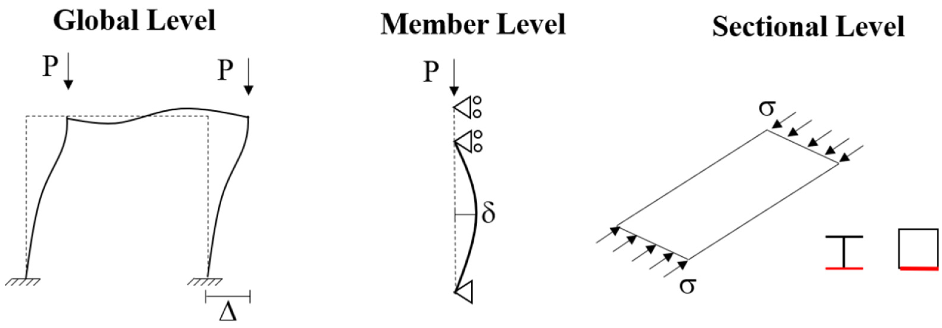
1. Introduction
In recent decades, the use of aluminium alloys has spread into many engineering fields. In fact, this material is successfully applied in transportation, such as in the rail industry (subway coaches, sleeping cars), automotive industry (car and moto components, moving cranes), and shipping industry (motorboats, sailboats). Aluminium alloys are also successfully used in the civil engineering field where they are employed both as a main element and as a secondary element within civil structures [1,2]. The main advantages of aluminium alloys are related to their lightness, corrosion resistance, and high functionality of structural shapes due to the extrusion process. For these reasons, aluminium material is competitive with steel in the application of structural design. However, used as structural material, it is affected by the same problems concerning the steel members, particularly the instability phenomena which can occur at different levels (Figure 1) and either in the elastic or plastic range. These phenomena are even more relevant in the case of aluminium structures, considering that the Young modulus of aluminium is about one third of that of the steel. In this paper, the attention is focused on studying the effect of local buckling effects on the ultimate response of aluminium members subjected to uniform compression or non-uniform flexural bending. Clearly, local and distortional buckling occurs when the portions of a single aluminium member are subjected to uniform or non-uniform compression. For this reason, the real prediction of the ultimate response of aluminium members becomes very complex and, generally, the proposed methodologies by the current codes underestimate their maximum capacity during compression or bending. Recently, Krishanun Roy et al. [3,4] highlighted that, in the case of channel section members, the design codes (Aluminium Design Manual [5] Australian/New Zealand Standards [6], Eurocode 9 [7] and Eurocode 3 [8]) are conservative within the 20–30% range, with respect to the experimental tests. The same problem was encountered by Feng et al. [9,10] in the case of the circular hollow sections of the aluminium alloy with holes during compression or bending. In the case of compression, the authors provided a new design equation based on the current design formulae that use the effective area method (EAM).

Figure 1.
Instability phenomena on the metal structures.
The excessive underestimation of the maximum capacity prediction is related to the current codes which consider only the elastic local buckling, which affects the ultimate resistance of the slender aluminium sections and neglects the interaction of the plate elements constituting the cross-sections and the strain-hardening behaviour of the aluminium alloys. Instead, for thicker sections, a plastic analysis is adopted in a similar way to the steel members. This approach leads to underestimated maximum capacity values with respect to the real behaviour of the aluminium material. Recently, in order to obtain more accurate predictions of the ultimate resistance of the aluminium sections, different approaches were presented within the scientific community. Su et al. [11] evaluated the applicability of the Continuous Strength Method (CSM), which was originally developed for stainless steel stocky (i.e., small width-to-thickness ratio) cross-sections. Zhu and Young [12] modified the current Direct Strength Method (DSM) to achieve more accurate design provisions for flexural SHS members, while Kim and Peköz [13] presented a simplified design approach called the Numerical Slenderness Approach (NSA) for determining the nominal stresses of each plate element of a complex section under flexure. In the case of aluminium box and H-shaped members, the same authors proposed simple mathematical formulations to predict the ultimate flexural resistance and rotation capacity as a function of the main nondimensional slenderness parameters [14,15,16,17,18,19]. These results are currently proposed in the Annex L of new Eurocode 9 draft [7].
Recently, starting from the effective thickness method (ETM) currently adopted by Eurocode 9, an extension of this approach is presented in [17], in order to compute the ultimate resistance of box-shaped members during compression or bending. The new version of ETM considers the plastic interactive buckling of cross-sections and the strain-hardening behaviour of aluminium material. In order to evaluate the accuracy of this simplified approach, a numerical application is provided. In particular, with reference to the box sections, the experimental results presented in [20,21,22] are compared with those obtained by the extension of the effective thickness method.
2. Different Approaches in the Design of Aluminium Section
In the technical literature, there are different simplified methods to evaluate the behaviour of aluminium members under uniform or non-uniform compression, taking into account that the response of thin-walled sections is strongly affected by local instability phenomena which arise in the compressed section. The main approaches, codified and adopted by the European Eurocodes, are: (1) the width effective approach, (2) the reduced strength approach, and (3) the effective thickness approach.
The first approach is very well known, being codified for many years with particular reference to steel structures [8]. It was first introduced by Von Kármán in 1932 [23]. He stated that, for a fixed thickness, a fictitious plate with the width of would have the critical stress equal to the yield stress. If the actual plate has a larger width, the capacity is the same as that of the fictitious plate. In a plate, the real stress distribution is approximated, or replaced, with two strips which describe the load-carrying, effective width of the plate. Consequently, this method is based on reducing the cross-section area in the parts affected by plate buckling.
The reduced stress method, used in the past in the Aluminium Associated Code [24], verifies the stress level at which a plate part buckles; if a cross-section is built up from multiple plate parts, the lowest stress governs the entire cross-section. Therefore, this method evaluates the capacities of a slender section by considering a reduced value of the limiting stress acting on the full section.
Finally, the effective thickness approach, first introduced in the British Code of Practice for Structural Aluminium [25], was recently introduced in EN1999-1-1, which concerns aluminium alloy structures [7]. This approach is based on replacing the true section with an effective section, obtained to reduce the actual thickness of the compressed parts. The main advantage of the effective thickness approach is that the influence of the heat-affected zones is more easily accounted for in the case of the cross-sections composed by welding. This is very important in the case of aluminium alloy structures where a significant reduction in the material properties arises in the heat-affected zones.
Figure 2 shows a qualitative comparison between the different design approaches for a generic box section subjected to non-uniform compression.
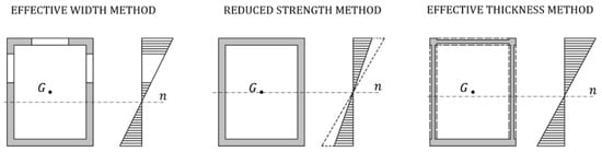
Figure 2.
Comparison of the different design approaches for a rectangular section in bending.
Nowadays, the current European Code Provisions suggest the use of the effective width approach and the effective thickness method for the steel and aluminium cross-section, respectively. In particular, these methods are indirectly used to evaluate the behaviour of the slender sections, belonging to class 4, affected by the local buckling occurring in the elastic region.
3. Extension of Effective Thickness Method (ETM)
3.1. Stability of a Single Plate in the Elastic-Plastic Region
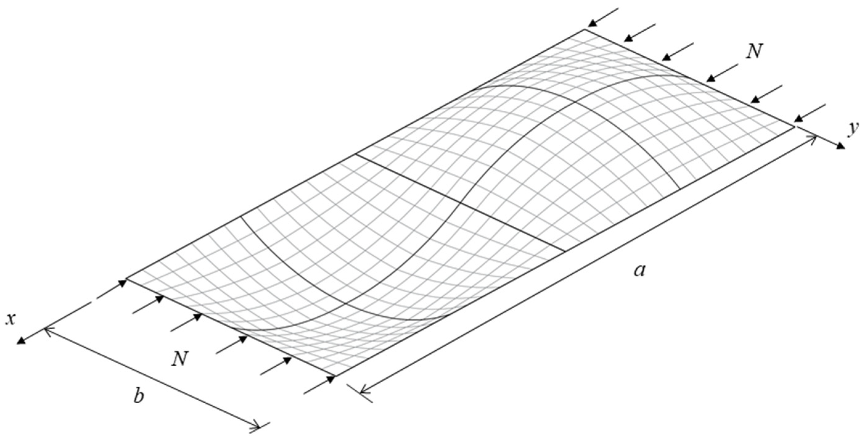
According to a single plate under uniform compression (Figure 3), the elastic critical stress is equal to:
where is the elastic modulus, is the Poisson’s ratio in the elastic range, is the plate width, is the length plate, is the plate thickness and is the buckling factor. The factor accounts for the edge-restraining conditions and the stress distribution along the loaded edges. In the case of the plate elements constituting the section of a structural member, the occurrence of elastic buckling is also affected by the interaction between the plate elements constituting the member section and by the longitudinal stress gradient. These effects can be considered by modifying Equation (1) using two factors: and . The factor accounts for the interaction between the plate elements that constitute the section, while the factor accounts for the influence of the longitudinal stress gradient occurring in the structural members under non-uniform bending. Clearly, in the case of uniform compression, . Therefore, including the effects of interactive buckling, the longitudinal stress gradient and the non-linear behaviour of material, the elastic buckling stress can be expressed, by rearranging Equation (1) in the following form:

Figure 3.
Single plate under uniform compression.
The correction factor for the interactive buckling can be evaluated by taking into account that it represents the ratio between the buckling factor , accounting for interactive buckling, and the buckling factor , evaluated for the isolated plate element, i.e., . The main expressions are provided by BS5950-5 [26], while, regarding the factor accounting for the influence of the longitudinal stress gradient , the relationships are presented in [27,28].
The occurrence of buckling in the plastic range can be accounted for using a correction factor that depends on the non-linear behaviour of the material. By denoting with such a correction factor, the buckling stress in the plastic range is given by:
Concerning the Poisson’s ratio in the yield region, Gerard and Wildhorn (1952) [29] studied the problem in the case of several aluminium alloys and showed that they were seriously affected by the anisotropy of the material. Therefore, they proposed the following expression:
where is the secant modulus and represents the Poisson’s ratio in the plastic range, which is equal to . Regarding the plastic coefficient , there are many expressions in the scientific literature [30]. The main relationships are reported in the following:
where is the tangent modulus and represents the exponent of the Ramberg–Osgood law that describes the behaviour of aluminium alloys. Recently, the use of a different formula was suggested by the same authors for the proposed Annex L of EN 1999-1-1:
| • tangent modulus theory | |
| • secant modulus theory | |
| • Pearson (1950), Bleich (1952), Vol’Mir (1965) | |
| • Gerard (1957) | |
| • Weingarten et al. (1960) | |
| • Stowell (1948), Bijlaard (1949) | |
| • Li and Reid (1992) |
It is easy to recognize that Equation (5) is a combination of the secant modulus theory with the Gerard formula. In particular, for the small values of the Ramberg–Osgood exponent , Equation (5) tends to provide values close to those given by Gerard. Conversely, for high values of n, Equation (5) tends to provide values close to the secant modulus theory.
3.2. Mathematical Steps for the Definition of the New Version of ETM
In this section, the mathematical steps, needed to compute the effective thickness in the non-linear range as a function of the strain level, are reported. In particular, Equation (3) can be rewritten as:
where is the strain corresponding to buckling. So, the effective ratio can be defined as a function of the strain level as:
The previous equation can be written as:
by introducing the parameter , which accounts the nonlinear behaviour of aluminium material:
Therefore, Equation (8) can be rewritten as:
remembering that:
where is the normalised slenderness in the elastic-plastic region. To use the buckling curves of Eurocode 9 [7], with the normalised slenderness corrected to account for the non-linearity depending on the strain level, it must be considered that:
where and represents the conventional yield stress of the aluminium material. Therefore:
The factor accounting for the stress distribution along the loaded edge is:
The final expression used to compute the slenderness parameter of the single-plate element to use with the buckling curves of EN1999-1-1 [7] is:
The last equation computes the effective thickness in the non-linear range as a function of the strain level . In fact, according to EN1999-1-1 [7], the reduction factor accounting for local buckling is computed as:
The parameter accounts for the strain distribution along the loaded edge of the plate. It is given by the ratio between the maximum compression strain at one end of the plate and the strain at the second end of the plate element. In the case of uniform compression, it is while when the second end of the plate element is subject to tension. Meanwhile, the values of coefficients and are reported in Eurocode 9 and they depend on the class of the buckling curves.
4. Numerical Application to the Box Sections
In this section, the numerical application is provided with reference to the box-shaped members under uniform compression or bending. The aluminium alloy, considered in this procedure, is EN-AW 6082 T6 and, according to the nominal mechanical proprieties presented in Eurocode 9, it is characterized by the conventional yield stress and the ultimate stress ; the exponent of Ramberg–Osgood is . The nominal Young modulus is assumed to be equal to while the geometric properties of the box section are the plate width equal to and the plate thickness equal to .
4.1. Box Sections under Uniform Compression
The application of the effective thickness approach, as previously described, requires a procedure under displacement control. Regarding the stub columns subjected to uniform compression, by increasing the values of the axial displacement , the corresponding average strain is derived; represents the height of members. Therefore, the slenderness parameter is given by Equation (14) for the increasing values of the strain level and computed for the plate elements constituting the member section. It increases with the increasing values of . The appropriate buckling curve is used, according to EN1999-1-1, so that the effective thickness is computed for all the plate elements and the effective cross-section area is computed. The axial force corresponding to the axial displacement is obtained as , where is the stress level corresponding to , evaluated according to the constitutive stress–strain curve of the material, i.e., the Ramberg–Osgood model:
It is important to underline that the aluminium material could be expressed with other mathematical models, for example a two stage R-O model, recently proposed by Yun et al. [31], which appears to be more suitable than the simple R-O law for use in analytical modelling, numerical simulations, and the advanced design of aluminium alloy structures.
The numerical procedure is performed step-by-step by means of the MATLAB program [32] and it is repeated by varying the plastic coefficient according to the relationships presented in Section 3.1.
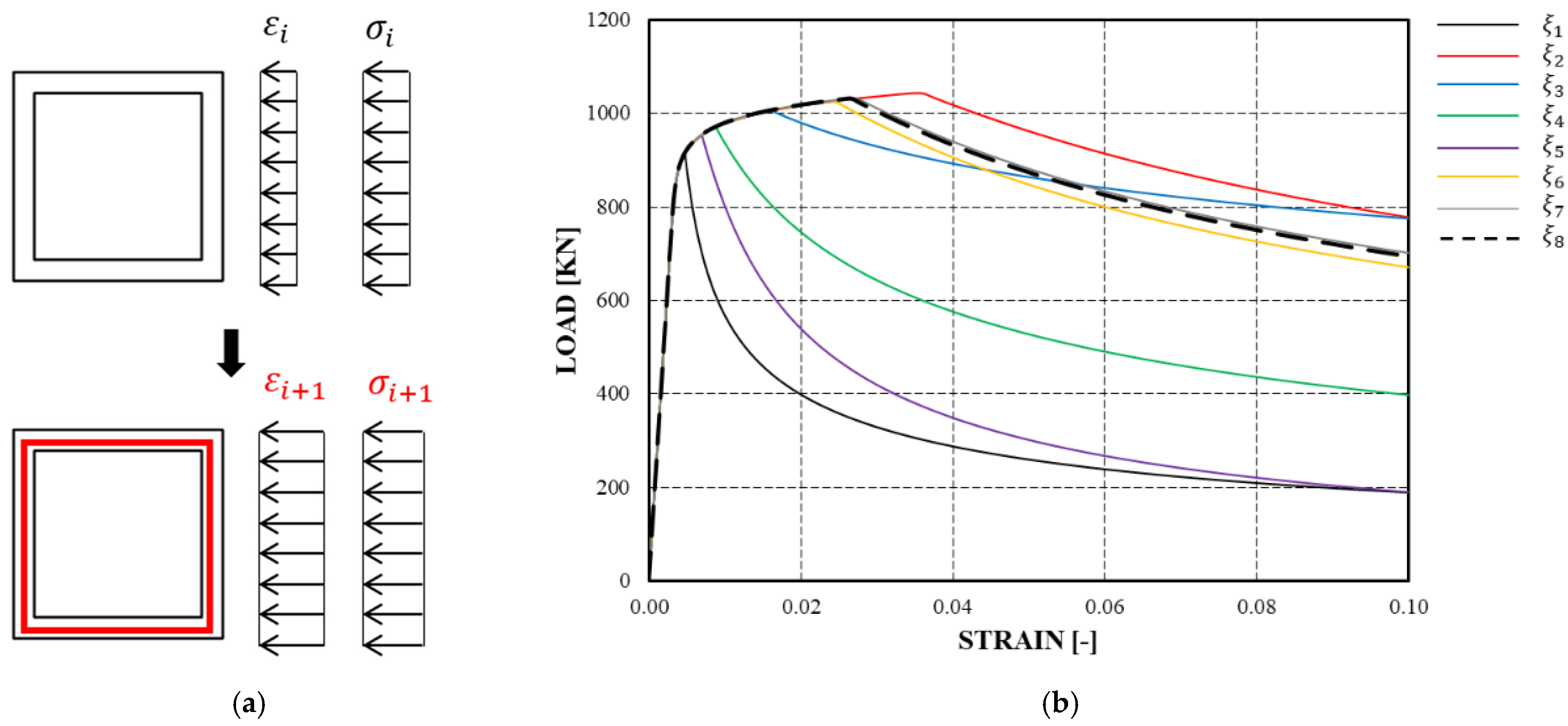
The generic steps of the procedure are shown in Figure 4a. At the initial step, a generic box section is subjected to the strain level and, consequently, to the stress level . At step , the strain level increases, and it is equal to , where the corresponding stress state is . By applying Equations (14) and (15), the effective thickness of the box section decreases (red line) with the definition of the reduction coefficient .
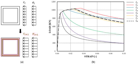
Figure 4.
Scheme of a generic box section in compression (a). The load-strain curves by varying the plastic coefficient (b).
In Figure 4b, the results of the numerical procedure are depicted in terms of the load–strain curves. It is possible to observe that the tangent modulus theory provides lower load values, while the higher values are obtained by means of the secant modulus theory ). Instead, the results provided by the new formulation, i.e., Equation (5), are located between the Stowell-Bijlaard ) and Li-Reid ) results.
4.2. Box Sections under Non-Uniform Bending Moment
The same procedure was repeated in the case of the box-shaped aluminium beam under the non-uniform bending moment. The mechanical and geometric properties are the same as those reported in Section 4.1 and, moreover, the beam length is assumed as equal to .
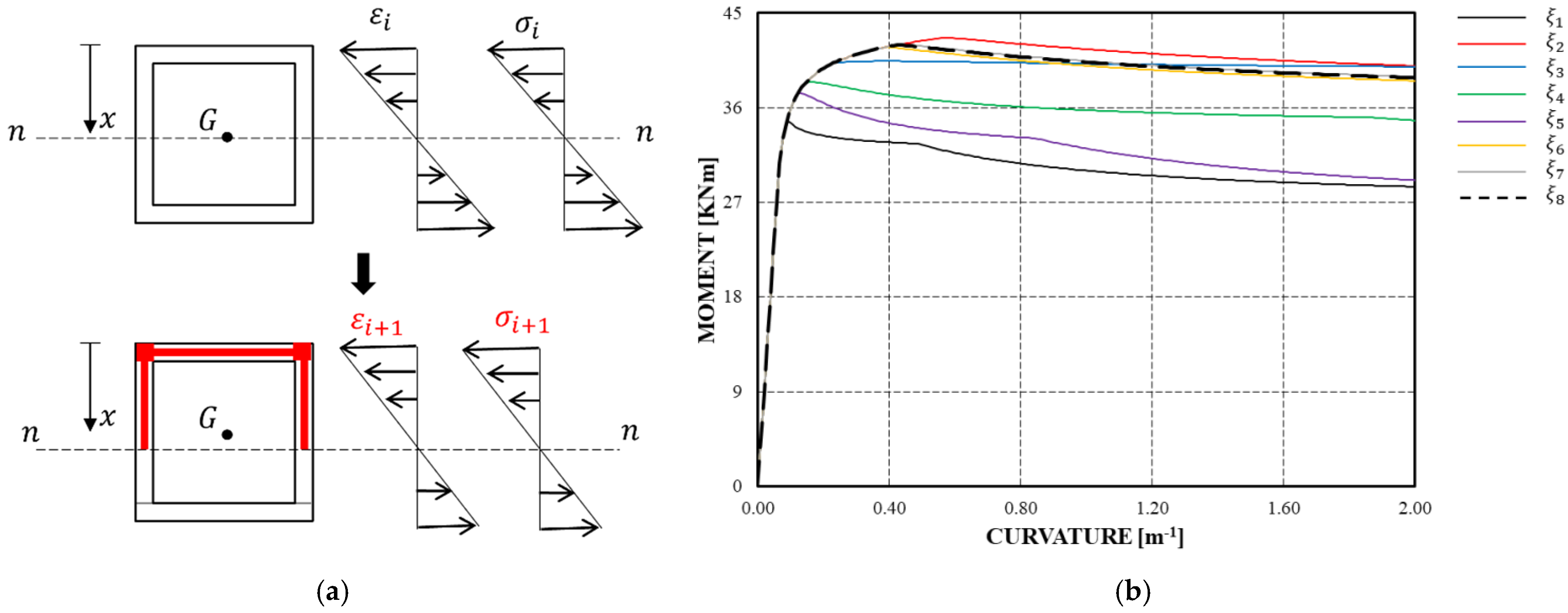
In this case, the iterative procedure is more complicated than the previous case. In fact, the strain level and, consequently, the corresponding stress , are not constant, but vary along the section height, as shown in Figure 5a. For this reason, it is not possible to apply a continuous relation, as depicted for the uniform compression, but a fiber model is used to evaluate the curvature as a function of the strain level . Finally, the bending moment is evaluated by means of the rotational equilibrium equation between the compression parts and the tension parts. Moreover, the rotation corresponding to the attainment of the flexural resistance was calculated by integrating the curvature diagram along the shear length of the structural member:
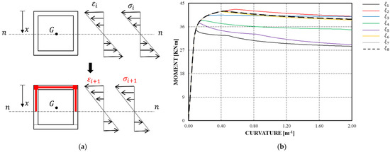
Figure 5.
Scheme of a generic box section in bending (a). The moment-curvature curves by varying the plastic coefficient (b).
Obviously, the rotation , can be estimated by means of Equation (18) for , i.e., the curvature corresponding to the maximum bending moment . Meanwhile, the maximum rotation , corresponding to the point where the moment resistance drops below the conventional yield value , can be computed as:
where is the ultimate curvature and is the length of the plastic hinge evaluated as the distance between the points where the conventional yield curvature and occurs.
The generic steps of the procedure are shown in Figure 5a, while in Figure 5b, the results of the numerical procedure are depicted in terms of the moment–curvature curves. The considerations, made in the case of uniform compression, are still valid for the box-shaped beam under a non-uniform bending moment.
5. Comparison with Experimental Tests
The accuracy of the previous methodology is evaluated by comparing the theoretical results with those provided in the scientific literature. The following analyses were performed by varying the plastic coefficient according to the relationships provided in Section 3. The numerical results are reported in Appendix B. In particular, in Table A3 and Table A5, the experimental and numerical values are shown in Table A3 and Table A5, while the ratio values are shown in Table A4 and Table A6. In the case of uniform compression, the theoretical results are compared with the stub column tests performed by Su et al. [21], while, in the case of bending moment, the theoretical values are compared with the results of the three-point bending tests performed by Moen et al. [20] and Su et al. [22]. For the sake of completeness, the experimental results were compared with those obtained by Eurocode 9, taking into account the local buckling effects for the fourth-class sections. The mean values, the standard deviations , and the variation coefficients of the ratios between the theoretical and experimental results are reported in Table A4 and Table A6.
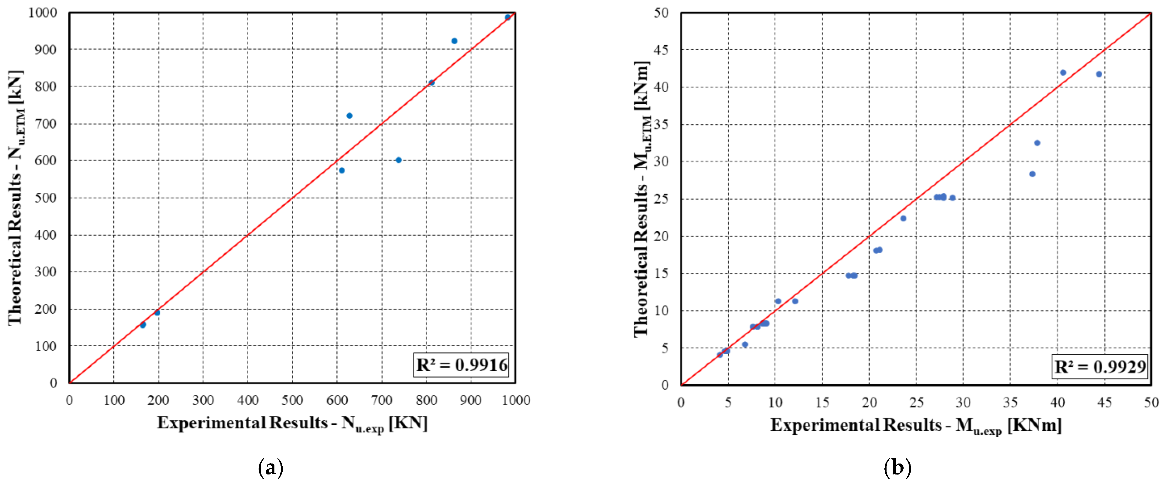
By the comparison between the experimental tests and the theoretical methodologies, it is possible to observe that the Eurocode 9 provides underestimated resistance values with respect to the experimental tests and, consequently, the new methodology results are more accurate. Moreover, by observing the theoretical values obtained by varying the plastic coefficient , it is evident that the new expression reported in Equation (5) provides the values of the maximum compressive load and ultimate flexural resistance, which are more similar to the real behaviour of the aluminium members. In fact, in the case of uniform compression, the mean value of the ratio is about 1.00, while the standard deviation is equal to 0.09. In the case of bending moment, the mean value of the ratio is about 0.96 with the standard deviation equal to 0.06. In Figure 6a,b, the comparison between the results of ETM with the plastic coefficient and the experimental results are reported, respectively, in the case of uniform compression and bending moment. Instead, as seen in the numerical application (Section 4), it is evident that the tangent modulus theory ( underestimates the resistance values, while the secant modulus theory overestimates them. The theories of Stowell-Bijlaard and Li-Reid provide the values very similar to the experimental one; however, from a stochastic point of view, they are characterized by a greater dispersion of the results.
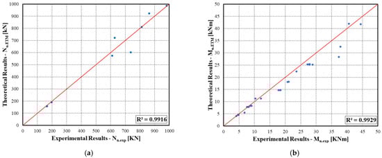
Figure 6.
Comparison between theoretical and experimental results in the case of uniform compression (a). Comparison between theoretical and experimental results in the case of non-uniform bending (b).
6. Conclusions
In this work, a numerical application of the extension of the effective thickness method (ETM) is presented. This approach was developed to define a simplified method to predict the ultimate behaviour of aluminium members in compression or in bending. The extension of ETM considers the strain-hardening behaviour of aluminium alloys, the interaction between plate elements constituting a generic cross-section, and, finally, the local buckling in the elastic-plastic region. In order to evaluate the influence of the plastic coefficient on the ultimate resistance of box-shaped aluminium members, an iterative procedure was performed by means of the MATLAB program. It was clear that the tangent modulus theory provided the lower values of the ultimate resistance, while the higher values were obtained by means of the secant modulus theory.
In order to consider the influence of the strain-hardening behaviour of aluminium alloys, a new formulation of the plastic coefficient was proposed. This relationship is a function of the Ramberg–Osgood exponent ; in this sense, it is the different inelastic behaviour which characterizes each aluminium alloy. The results provided by the new formulation are located between the Stowell-Bijlaard and Li-Reid results.
For evaluating the accuracy of this procedure, a comparison between the numerical results with those presented in the scientific literature is provided. The theoretical results were computed according to Eurocode 9 and the new version of ETM by varying the plastic coefficients.
The values of the ultimate resistance computed by the new methodology are more similar to the corresponding experimental values. Specifically, by comparing the results, it is evident that the Eurocode 9 approach underestimates the maximum resistance of the aluminium members both during compression and bending. Consequently, the current code has a safety advantage, but the aluminium alloys may be uncompetitive from the economic and design point of view. Conversely, the new approach provides the maximum resistance values similar to the experimental results. In fact, in the case of uniform compression, the mean values of the ratios are nearly 1.00, except when the plastic coefficient is computed by means of the tangent modulus theory or Weingarten theory . In case of the prediction of the flexural resistance, the mean values of the ratios are almost greater than 0.90. Additionally, in this case, when the plastic coefficient is computed by means of the tangent modulus theory or Weingarten theory , the theoretical values are underestimated with respect to the experimental results.
Additionally, the theoretical values obtained by applying the new formulation of the plastic coefficient are more accurate. In fact, the mean value, and the standard deviation of the ratio between the experimental and theoretical results are equal to 0.99 and 0.09 in the case of uniform compression and 0.96 and 0.06 for the beams during bending. Therefore, the new formulation (Equation (5)) provides the theoretical results with a very low dispersion index both during compression and bending.
Consequently, we can conclude that the new version of the effective thickness approach is valid and more accurate for predicting the maximum resistance of box-shaped aluminium members during compression or bending.
In a future development, for evaluating the accuracy of this method to predict the maximum deformation capacity of the members during compression or bending, stub column tests and three-point bending tests could be performed to compare the theoretical load–strain and bending-curvature curves with directly experimental ones. Moreover, in order to define a general procedure to be adopted within the design codes, this new version of ETM and its numerical applications could be extended to the other cross-sections (H-shaped, channel and angle sections) and other aluminium alloys with different heat-treatments.
Author Contributions
Conceptualization, V.P. and A.P.; methodology, V.P. and A.P.; software, A.P.; validation, A.P., V.P. and E.N.; formal analysis, A.P.; investigation, A.P.; resources, A.P.; data curation, A.P.; writing—original draft preparation, A.P., writing—review and editing, E.N.; visualization, A.P.; supervision, E.N. and V.P. All authors have read and agreed to the published version of the manuscript.
Funding
This research received no external funding.
Conflicts of Interest
The authors declare no conflict of interest.
Appendix A
According to Figure A1, the main mechanical and geometrical properties of the specimens, considered in the comparison with the theoretical results, are collected in the following Table A1 and Table A2:
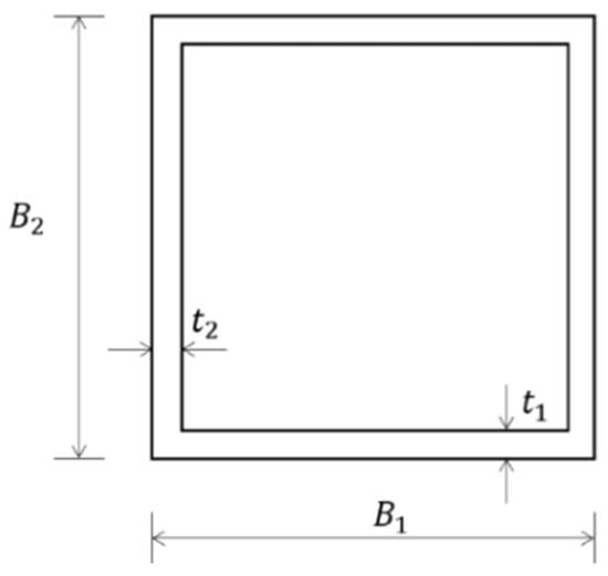
Figure A1.
Geometric scheme of box section.
Figure A1.
Geometric scheme of box section.


Table A1.
Experimental properties of stub column tests.
Table A1.
Experimental properties of stub column tests.
| Specimen | Alloy | B1 [mm] | t1 [mm] | B2 [mm] | t2 [mm] | a [mm] | A [mm2] | E [MPa] | f0.2 [MPa] | fu [MPa] | n [-] | |
|---|---|---|---|---|---|---|---|---|---|---|---|---|
| H64 × 64 × 3 | A | 6061 T6 | 63.90 | 2.81 | 63.90 | 2.81 | 191.10 | 686.65 | 66,000 | 234 | 248 | 12 |
| B | 6061 T6 | 63.90 | 2.85 | 63.90 | 2.85 | 191.50 | 695.97 | 66,000 | 234 | 248 | 12 | |
| H70 × 55 × 4.2 | A | 6061 T6 | 69.90 | 4.08 | 54.90 | 4.08 | 209.80 | 951.78 | 65,000 | 193 | 207 | 22 |
| B | 6061 T6 | 69.90 | 4.09 | 54.90 | 4.09 | 209.90 | 953.95 | 65,000 | 193 | 207 | 22 | |
| H95 × 50 × 10.5 | A | 6061 T6 | 94.80 | 10.36 | 49.70 | 10.36 | 284.90 | 2564.72 | 71,000 | 229 | 242 | 11 |
| H120 × 70 × 10.5 | A | 6061 T6 | 119.90 | 10.39 | 69.90 | 10.39 | 360.00 | 3512.24 | 69,000 | 226 | 238 | 10 |
| H120 × 120 × 9 | A | 6061 T6 | 120.00 | 8.91 | 120.00 | 8.91 | 360.20 | 3959.25 | 65,000 | 225 | 234 | 13 |
| N95 × 50 × 10.5 | A | 6063 T5 | 94.90 | 10.37 | 49.70 | 10.37 | 285.20 | 2568.86 | 69,000 | 179 | 220 | 10 |
| N120 × 70 × 10.5 | A | 6063 T5 | 119.90 | 10.45 | 69.80 | 10.45 | 360.90 | 3527.92 | 71,000 | 139 | 194 | 9 |
| N120 × 120 × 9 | A | 6063 T5 | 120.00 | 8.92 | 120.00 | 8.92 | 361.30 | 3963.33 | 69,000 | 181 | 228 | 9 |
Table A2.
Experimental properties of three-point bending tests.
Table A2.
Experimental properties of three-point bending tests.
| Specimen | Alloy | B1 [mm] | t1 [mm] | B2 [mm] | t2 [mm] | L [mm] | A [mm2] | E [MPa] | f0.2 [MPa] | fu [MPa] | n [-] |
|---|---|---|---|---|---|---|---|---|---|---|---|
| Q1-1m-1 | 6082 T6 | 99.60 | 5.94 | 100.30 | 5.89 | 1000 | 2224 | 68,886 | 315.50 | 323.50 | 64.0 |
| Q1-1m-2 | 6082 T6 | 99.60 | 5.94 | 100.30 | 5.89 | 1000 | 2224 | 68,886 | 315.50 | 323.50 | 64.0 |
| Q1-2m-1 | 6082 T6 | 99.60 | 5.94 | 100.30 | 5.89 | 2000 | 2224 | 68,886 | 315.50 | 323.50 | 64.0 |
| Q1-2m-3 | 6082 T6 | 99.60 | 5.94 | 100.30 | 5.89 | 2000 | 2224 | 68,886 | 315.50 | 323.50 | 64.0 |
| Q2-1m-1 | 6082 T4 | 100.00 | 5.95 | 100.00 | 5.88 | 1000 | 2225 | 66,868 | 176.60 | 283.40 | 38.0 |
| Q2-1m-2 | 6082 T4 | 100.00 | 5.95 | 100.00 | 5.88 | 2000 | 2225 | 66,868 | 176.60 | 283.40 | 38.0 |
| Q2-2m-1 | 6082 T4 | 100.00 | 5.95 | 100.00 | 5.88 | 2000 | 2225 | 66,868 | 176.60 | 283.40 | 38.0 |
| Q2-2m-2 | 6082 T4 | 100.00 | 2.89 | 99.70 | 2.83 | 1000 | 1110 | 66,853 | 120.10 | 221.00 | 26.0 |
| Q3-1m-1 | 6082 T4 | 100.00 | 2.89 | 99.70 | 2.83 | 1000 | 1110 | 66,853 | 120.10 | 221.00 | 26.0 |
| Q3-1m-3 | 6082 T4 | 100.00 | 2.89 | 99.70 | 2.83 | 2000 | 1110 | 66,853 | 120.10 | 221.00 | 26.0 |
| Q3-2m-1 | 6082 T4 | 100.00 | 2.89 | 99.70 | 2.83 | 2000 | 1110 | 66,853 | 120.10 | 221.00 | 26.0 |
| Q3-2m-2 | 6082 T4 | 100.10 | 5.94 | 100.00 | 5.98 | 2000 | 2243 | 66,880 | 314.00 | 333.40 | 65.0 |
| Q4-2m-1 | 7108-T7 | 100.10 | 5.94 | 100.00 | 5.98 | 2000 | 2243 | 66,880 | 314.00 | 333.40 | 65.0 |
| Q4-2m-2 | 7108-T7 | 60.00 | 2.29 | 119.40 | 2.58 | 1000 | 867 | 66,577 | 288.50 | 302.30 | 51.0 |
| R1-1m-1 | 6082 T6 | 60.00 | 2.29 | 119.40 | 2.58 | 2000 | 867 | 66,577 | 288.50 | 302.30 | 51.0 |
| R1-2m-1 | 6082 T6 | 60.00 | 2.29 | 119.40 | 2.58 | 2000 | 867 | 66,577 | 288.50 | 302.30 | 51.0 |
| R1-2m-2 | 6082 T6 | 60.00 | 2.29 | 119.40 | 2.58 | 3000 | 867 | 66,577 | 288.50 | 302.30 | 51.0 |
| R1-3m-1 | 6082 T6 | 60.00 | 2.29 | 119.40 | 2.58 | 3000 | 867 | 66,577 | 288.50 | 302.30 | 51.0 |
| R1-3m-2 | 6082 T6 | 60.10 | 2.94 | 100.00 | 2.94 | 1000 | 906 | 66,225 | 281.40 | 290.40 | 45.0 |
| R2-1m-1 | 6082 T6 | 60.10 | 2.94 | 100.00 | 2.94 | 1000 | 906 | 66,225 | 281.40 | 290.40 | 45.0 |
| R2-1m-2 | 6082 T6 | 60.10 | 2.94 | 100.00 | 2.94 | 2000 | 906 | 66,225 | 281.40 | 290.40 | 45.0 |
| R2-2m-1 | 6082 T6 | 60.10 | 2.94 | 100.00 | 2.94 | 2000 | 906 | 66,225 | 281.40 | 290.40 | 45.0 |
| R2-2m-2 | 6082 T6 | 60.10 | 2.94 | 100.00 | 2.94 | 3000 | 906 | 66,225 | 281.40 | 290.40 | 45.0 |
| R2-3m-1 | 6082 T6 | 60.10 | 2.94 | 100.00 | 2.94 | 3000 | 906 | 66,225 | 281.40 | 290.40 | 45.0 |
| R2-3m-2 | 6082 T6 | 69.80 | 4.09 | 55.20 | 4.09 | 695 | 906 | 67,000 | 207.00 | 222.00 | 16.0 |
| H55 × 70 × 4B3 | 6061 T6 | 54.70 | 4.09 | 69.80 | 4.09 | 693 | 956 | 67,000 | 207.00 | 222.00 | 16.0 |
| H95 × 50 × 10B3 | 6061 T6 | 94.70 | 10.34 | 49.60 | 10.34 | 695 | 951 | 68,000 | 229.00 | 242.00 | 11.0 |
| H50 × 95 × 10B3 | 6061 T6 | 49.50 | 10.34 | 94.60 | 10.34 | 693 | 2556 | 68,000 | 229.00 | 242.00 | 11.0 |
| H64 × 64 × 3B3 | 6061 T6 | 63.90 | 2.89 | 63.80 | 2.89 | 693 | 2552 | 67,000 | 232.00 | 245.00 | 10.0 |
| H120 × 120 × 9xB3 | 6061 T6 | 120.00 | 8.90 | 119.90 | 8.90 | 691 | 705 | 65,000 | 225.00 | 234.00 | 13.0 |
| H120 × 70 × 10xB3 | 6061 T6 | 119.80 | 10.28 | 69.80 | 10.28 | 691 | 3953 | 68,000 | 226.00 | 238.00 | 10.0 |
| H70 × 120 × 10xB4 | 6061 T6 | 69.80 | 10.26 | 119.80 | 10.26 | 692 | 3475 | 68,000 | 226.00 | 238.00 | 10.0 |
| H70 × 55 × 4B3-R | 6061 T6 | 69.80 | 4.07 | 54.80 | 4.07 | 694 | 3470 | 65,000 | 193.00 | 207.00 | 22.0 |
| H50 × 95 × 10B3-R | 6061 T6 | 49.50 | 10.33 | 94.70 | 10.33 | 693 | 948 | 68,000 | 229.00 | 242.00 | 11.0 |
| H64 × 64 × 3B3-R | 6061 T6 | 63.90 | 2.83 | 63.90 | 2.83 | 696 | 2552 | 67,000 | 232.00 | 245.00 | 10.0 |
| N120 × 70 × 10B3 | 6063 T5 | 120.00 | 10.40 | 69.90 | 10.40 | 689 | 691 | 71,000 | 139.00 | 194.00 | 9.0 |
| N70 × 120 × 10B3 | 6063 T5 | 69.90 | 10.40 | 119.90 | 10.40 | 688 | 3517 | 71,000 | 139.00 | 194.00 | 9.0 |
| N120 × 120 × 9B3 | 6063 T5 | 119.90 | 8.90 | 119.90 | 8.90 | 693 | 3515 | 69,000 | 181.00 | 228.00 | 9.0 |
Appendix B
In this section, the numerical comparison between the theoretical and experimental results are collected in the following tables. In particular, the experimental results presented in the scientific literature are reported in the first column; the theoretical results computed according to Eurocode 9 are listed in the second column. In the last columns, the values derived by the new version of ETM are reported in the last columns. Specifically, they are computed by varying the plastic coefficients according to the relationships provided in Section 3. Moreover, the mean value [, the standard deviation and the coefficient of variation of the ratio between the theoretical and experimental results are reported in the final part of Table A4 and Table A6.
Table A3.
Comparison between the theoretical and experimental results in the case of uniform compression.
Table A3.
Comparison between the theoretical and experimental results in the case of uniform compression.
| Specimen | Nu.exp [kN] | Nu.EC9 [kN] | Nu.ETM [kN] | ||||||||
|---|---|---|---|---|---|---|---|---|---|---|---|
| ξ1 | ξ2 | ξ3 | ξ4 | ξ5 | ξ6 | ξ7 | ξ8 | ||||
| H64 × 64 × 3 | A | 164.2 | 150.68 | 129.07 | 154.95 | 138.10 | 136.50 | 135.18 | 145.12 | 147.57 | 158.13 |
| B | 165.4 | 152.86 | 131.54 | 158.33 | 141.07 | 139.34 | 137.92 | 148.37 | 150.87 | 160.54 | |
| H70 × 55 × 4.2 | A | 196.2 | 183.69 | 167.99 | 193.69 | 179.37 | 176.82 | 175.13 | 188.61 | 190.26 | 191.31 |
| B | 196.9 | 184.11 | 168.37 | 194.30 | 179.82 | 177.37 | 175.53 | 189.21 | 190.79 | 191.74 | |
| H95 × 50 × 10.5 | A | 626.2 | 587.32 | 620.66 | 776.37 | 783.85 | 690.55 | 651.70 | 750.18 | 757.69 | 722.86 |
| H120 × 70 × 10.5 | A | 862.5 | 793.77 | 795.71 | 1008.01 | 980.70 | 886.35 | 843.13 | 968.12 | 979.62 | 924.23 |
| H120 × 120 × 9 | A | 981.5 | 890.83 | 839.36 | 1027.42 | 959.40 | 914.06 | 888.85 | 991.79 | 1001.69 | 987.83 |
| N95 × 50 × 10.5 | A | 609.8 | 459.83 | 494.87 | 626.53 | 649.24 | 554.78 | 516.96 | 603.68 | 610.10 | 574.76 |
| N120 × 70 × 10.5 | A | 736.9 | 490.38 | 504.22 | 646.89 | 667.38 | 568.00 | 528.23 | 620.91 | 627.97 | 603.69 |
| N120 × 120 × 9 | A | 811.1 | 717.36 | 693.58 | 889.77 | 857.29 | 774.95 | 735.97 | 850.14 | 861.62 | 812.48 |
Table A4.
Ratio values between the theoretical and experimental results in the case of uniform compression.
Table A4.
Ratio values between the theoretical and experimental results in the case of uniform compression.
| Specimen | Nu.EC9/Nu.exp | Nu.ETM/Nu.exp | ||||||||
|---|---|---|---|---|---|---|---|---|---|---|
| ξ1 | ξ2 | ξ3 | ξ4 | ξ5 | ξ6 | ξ7 | ξ8 | |||
| H64 × 64 × 3 | A | 0.92 | 0.79 | 0.94 | 0.84 | 0.83 | 0.82 | 0.88 | 0.90 | 0.96 |
| B | 0.92 | 0.80 | 0.96 | 0.85 | 0.84 | 0.83 | 0.90 | 0.91 | 0.97 | |
| H70 × 55 × 4.2 | A | 0.94 | 0.86 | 0.99 | 0.91 | 0.90 | 0.89 | 0.96 | 0.97 | 0.98 |
| B | 0.94 | 0.86 | 0.99 | 0.91 | 0.90 | 0.89 | 0.96 | 0.97 | 0.97 | |
| H95 × 50 × 10.5 | A | 0.94 | 0.99 | 1.24 | 1.25 | 1.10 | 1.04 | 1.20 | 1.21 | 1.15 |
| H120 × 70 × 10.5 | A | 0.92 | 0.92 | 1.17 | 1.14 | 1.03 | 0.98 | 1.12 | 1.14 | 1.07 |
| H120 × 120 × 9 | A | 0.91 | 0.86 | 1.05 | 0.98 | 0.93 | 0.91 | 1.01 | 1.02 | 1.01 |
| N95 × 50 × 10.5 | A | 0.75 | 0.81 | 1.03 | 1.06 | 0.91 | 0.85 | 0.99 | 1.00 | 0.94 |
| N120 × 70 × 10.5 | A | 0.67 | 0.68 | 0.88 | 0.91 | 0.77 | 0.72 | 0.84 | 0.85 | 0.82 |
| N120 × 120 × 9 | A | 0.88 | 0.86 | 1.10 | 1.06 | 0.96 | 0.91 | 1.05 | 1.06 | 1.00 |
| Mean value [μ]: | 0.88 | 0.84 | 1.03 | 0.99 | 0.92 | 0.88 | 0.99 | 1.00 | 0.99 | |
| Standard deviation [σ]: | 0.09 | 0.08 | 0.11 | 0.13 | 0.10 | 0.09 | 0.11 | 0.11 | 0.09 | |
| Coefficient of variation [COV]: | 0.11 | 0.10 | 0.11 | 0.13 | 0.10 | 0.10 | 0.11 | 0.11 | 0.09 | |
Table A5.
Comparison between the theoretical and experimental results in the case of bending moment.
Table A5.
Comparison between the theoretical and experimental results in the case of bending moment.
| Specimen | Mu.exp [kNm] | Mu.EC9 [kNm] | Mu.ETM [kNm] | |||||||
|---|---|---|---|---|---|---|---|---|---|---|
| ξ1 | ξ2 | ξ3 | ξ4 | ξ5 | ξ6 | ξ7 | ξ8 | |||
| H70 × 55 × 4.2B3 | 4.75 | 4.16 | 4.76 | 6.09 | 5.64 | 5.18 | 4.94 | 4.94 | 5.48 | 4.75 |
| H55 × 70 × 4.2B3 | 6.76 | 4.63 | 4.70 | 5.10 | 4.83 | 4.81 | 4.64 | 4.64 | 4.72 | 6.56 |
| H95 × 50 × 10.5B3 | 12.09 | 12.68 | 12.91 | 13.91 | 12.91 | 12.91 | 12.84 | 12.84 | 12.91 | 11.33 |
| H50 × 95 × 10.5B3 | 21.09 | 17.05 | 23.63 | 25.04 | 24.07 | 23.74 | 23.57 | 23.57 | 23.95 | 19.25 |
| H64 × 64 × 3.0B3 | 4.1 | 3.72 | 4.10 | 4.56 | 4.49 | 4.30 | 4.12 | 4.12 | 4.35 | 4.17 |
| H120 × 120 × 9.0xB3 | 44.42 | 38.47 | 45.36 | 46.35 | 41.42 | 42.27 | 42.64 | 45.64 | 46.34 | 41.79 |
| H120 × 70 × 10.50xB3 | 23.59 | 22.92 | 25.36 | 26.35 | 26.42 | 26.27 | 25.64 | 25.64 | 26.34 | 22.41 |
| H70 × 120 × 10.50xB4 | 37.86 | 29.53 | 37.93 | 37.91 | 37.93 | 37.93 | 37.59 | 37.59 | 37.92 | 32.63 |
| H70 × 55 × 4.2B3-R | 4.82 | 3.83 | 4.29 | 4.49 | 4.29 | 4.29 | 4.18 | 4.18 | 4.29 | 4.75 |
| H64 × 64 × 3.0B3-R | 10.28 | 3.65 | 3.55 | 4.05 | 3.98 | 3.66 | 3.49 | 3.49 | 3.86 | 11.33 |
| N120 × 70 × 10.5B3 | 20.72 | 14.3 | 16.43 | 20.36 | 21.39 | 17.92 | 16.40 | 16.40 | 19.79 | 18.17 |
| N70 × 120 × 10.5B3 | 37.3 | 18.43 | 16.38 | 31.02 | 31.30 | 28.96 | 26.01 | 26.01 | 30.80 | 29.36 |
| N120 × 120 × 9.0B3 | 40.53 | 30.93 | 26.60 | 42.40 | 43.03 | 38.20 | 35.11 | 41.11 | 41.45 | 42.01 |
| Q1-1m-1 | 27.87 | 22.42 | 23.41 | 27.74 | 24.59 | 24.21 | 24.11 | 26.11 | 27.06 | 25.44 |
| Q1-1m-2 | 27.87 | 22.42 | 23.41 | 27.74 | 24.59 | 24.21 | 24.11 | 24.11 | 27.06 | 25.44 |
| Q1-2m-1 | 27.15 | 22.42 | 23.41 | 27.63 | 24.48 | 24.07 | 23.97 | 24.97 | 26.92 | 25.32 |
| Q1-2m-3 | 27.39 | 22.42 | 23.41 | 27.63 | 24.48 | 24.07 | 23.97 | 24.97 | 26.92 | 25.32 |
| Q2-1m-1 | 18.43 | 12.55 | 16.53 | 19.27 | 17.47 | 16.99 | 16.76 | 17.76 | 18.95 | 16.78 |
| Q2-1m-2 | 18.3 | 12.55 | 16.53 | 19.27 | 17.47 | 16.99 | 16.76 | 17.76 | 18.95 | 16.78 |
| Q2-2m-1 | 17.76 | 12.55 | 16.53 | 19.27 | 17.47 | 16.99 | 16.76 | 17.76 | 18.95 | 16.78 |
| Q2-2m-2 | 18.3 | 12.55 | 16.53 | 19.27 | 17.47 | 16.99 | 16.76 | 17.76 | 18.95 | 16.78 |
| Q3-1m-1 | 4.78 | 4.3 | 3.76 | 4.76 | 4.40 | 4.15 | 4.05 | 4.05 | 4.43 | 4.67 |
| Q3-1m-3 | 4.69 | 4.3 | 3.75 | 4.74 | 4.38 | 4.13 | 4.03 | 4.03 | 4.43 | 4.67 |
| Q3-2m-1 | 4.64 | 4.3 | 3.75 | 4.74 | 4.38 | 4.13 | 4.03 | 4.03 | 4.43 | 4.65 |
| Q3-2m-2 | 4.87 | 4.3 | 3.75 | 4.74 | 4.38 | 4.13 | 4.03 | 4.03 | 4.43 | 4.65 |
| Q4-2m-1 | 28.81 | 22.39 | 22.90 | 27.55 | 24.18 | 24.11 | 24.04 | 25.04 | 26.82 | 25.22 |
| Q4-2m-2 | 27.85 | 22.39 | 22.90 | 27.55 | 24.18 | 24.11 | 24.04 | 25.04 | 26.82 | 25.22 |
| R1-1m-1 | 8.1 | 7.53 | 7.62 | 9.14 | 8.28 | 8.13 | 8.01 | 8.31 | 8.98 | 7.90 |
| R1-2m-1 | 8.1 | 7.53 | 7.62 | 9.14 | 8.28 | 8.13 | 8.01 | 8.31 | 8.98 | 7.86 |
| R1-2m-2 | 8.1 | 7.53 | 7.62 | 9.13 | 8.27 | 8.13 | 8.00 | 8.31 | 8.97 | 7.86 |
| R1-3m-1 | 7.62 | 7.53 | 7.62 | 9.13 | 8.27 | 8.13 | 8.00 | 8.31 | 8.97 | 7.85 |
| R1-3m-2 | 7.54 | 7.53 | 6.96 | 8.65 | 7.85 | 7.60 | 7.40 | 7.80 | 8.45 | 7.85 |
| R2-1m-1 | 8.65 | 7.22 | 6.96 | 8.65 | 7.85 | 7.60 | 7.40 | 7.80 | 8.45 | 8.35 |
| R2-1m-2 | 8.65 | 7.22 | 6.96 | 8.62 | 7.83 | 7.58 | 7.38 | 7.78 | 8.42 | 8.35 |
| R2-2m-1 | 8.58 | 7.22 | 6.96 | 8.62 | 7.83 | 7.58 | 7.38 | 7.78 | 8.42 | 8.33 |
| R2-2m-2 | 8.8 | 7.22 | 6.96 | 8.61 | 7.82 | 7.57 | 7.38 | 7.88 | 8.41 | 8.33 |
| R2-3m-1 | 9.03 | 7.22 | 6.96 | 8.61 | 7.82 | 7.57 | 7.38 | 7.88 | 8.41 | 8.33 |
| R2-3m-2 | 8.95 | 7.22 | 6.96 | 8.61 | 7.82 | 7.57 | 7.38 | 7.88 | 8.41 | 8.33 |
Table A6.
Ratio values between the theoretical and experimental results in the case of bending moment.
Table A6.
Ratio values between the theoretical and experimental results in the case of bending moment.
| Specimen | Mu.EC9/Mu.exp | Mu.ETM/Mu.exp | |||||||
|---|---|---|---|---|---|---|---|---|---|
| ξ1 | ξ2 | ξ3 | ξ4 | ξ5 | ξ6 | ξ7 | ξ8 | ||
| H70 × 55 × 4.2B3 | 0.88 | 1.00 | 1.28 | 1.19 | 1.09 | 1.04 | 1.04 | 1.15 | 1.00 |
| H55 × 70 × 4.2B3 | 0.68 | 0.70 | 0.75 | 0.71 | 0.71 | 0.69 | 0.69 | 0.70 | 0.97 |
| H95 × 50 × 10.5B3 | 1.05 | 1.07 | 1.15 | 1.07 | 1.07 | 1.06 | 1.06 | 1.07 | 0.94 |
| H50 × 95 × 10.5B3 | 0.81 | 1.12 | 1.19 | 1.14 | 1.13 | 1.12 | 1.12 | 1.14 | 0.91 |
| H64 × 64 × 3.0B3 | 0.91 | 1.00 | 1.11 | 1.10 | 1.05 | 1.01 | 1.01 | 1.06 | 1.02 |
| H120 × 120 × 9.0xB3 | 0.87 | 1.02 | 1.04 | 0.93 | 0.95 | 0.96 | 1.03 | 1.04 | 0.94 |
| H120 × 70 × 10.50xB3 | 0.97 | 1.08 | 1.12 | 1.12 | 1.11 | 1.09 | 1.09 | 1.12 | 0.95 |
| H70 × 120 × 10.50xB4 | 0.78 | 1.00 | 1.00 | 1.00 | 1.00 | 0.99 | 0.99 | 1.00 | 0.86 |
| H70 × 55 × 4.2B3-R | 0.79 | 0.89 | 0.93 | 0.89 | 0.89 | 0.87 | 0.87 | 0.89 | 0.99 |
| H64 × 64 × 3.0B3-R | 0.36 | 0.35 | 0.39 | 0.39 | 0.36 | 0.34 | 0.34 | 0.38 | 1.10 |
| N120 × 70 × 10.5B3 | 0.69 | 0.79 | 0.98 | 1.03 | 0.86 | 0.79 | 0.79 | 0.95 | 0.88 |
| N70 × 120 × 10.5B3 | 0.49 | 0.44 | 0.83 | 0.84 | 0.78 | 0.70 | 0.70 | 0.83 | 0.79 |
| N120 × 120 × 9.0B3 | 0.76 | 0.66 | 1.05 | 1.06 | 0.94 | 0.87 | 1.01 | 1.02 | 1.04 |
| Q1-1m-1 | 0.80 | 0.84 | 1.00 | 0.88 | 0.87 | 0.87 | 0.94 | 0.97 | 0.91 |
| Q1-1m-2 | 0.80 | 0.84 | 1.00 | 0.88 | 0.87 | 0.87 | 0.87 | 0.97 | 0.91 |
| Q1-2m-1 | 0.83 | 0.86 | 1.02 | 0.90 | 0.89 | 0.88 | 0.92 | 0.99 | 0.93 |
| Q1-2m-3 | 0.82 | 0.85 | 1.01 | 0.89 | 0.88 | 0.88 | 0.91 | 0.98 | 0.92 |
| Q2-1m-1 | 0.68 | 0.90 | 1.05 | 0.95 | 0.92 | 0.91 | 0.96 | 1.03 | 0.91 |
| Q2-1m-2 | 0.69 | 0.90 | 1.05 | 0.95 | 0.93 | 0.92 | 0.97 | 1.04 | 0.92 |
| Q2-2m-1 | 0.71 | 0.93 | 1.09 | 0.98 | 0.96 | 0.94 | 1.00 | 1.07 | 0.94 |
| Q2-2m-2 | 0.69 | 0.90 | 1.05 | 0.95 | 0.93 | 0.92 | 0.97 | 1.04 | 0.92 |
| Q3-1m-1 | 0.90 | 0.79 | 1.00 | 0.92 | 0.87 | 0.85 | 0.85 | 0.93 | 0.98 |
| Q3-1m-3 | 0.92 | 0.80 | 1.01 | 0.93 | 0.88 | 0.86 | 0.86 | 0.95 | 1.00 |
| Q3-2m-1 | 0.93 | 0.81 | 1.02 | 0.94 | 0.89 | 0.87 | 0.87 | 0.96 | 1.00 |
| Q3-2m-2 | 0.88 | 0.77 | 0.97 | 0.90 | 0.85 | 0.83 | 0.83 | 0.91 | 0.95 |
| Q4-2m-1 | 0.78 | 0.79 | 0.96 | 0.84 | 0.84 | 0.83 | 0.87 | 0.93 | 0.88 |
| Q4-2m-2 | 0.80 | 0.82 | 0.99 | 0.87 | 0.87 | 0.86 | 0.90 | 0.96 | 0.91 |
| R1-1m-1 | 0.93 | 0.94 | 1.13 | 1.02 | 1.00 | 0.99 | 1.03 | 1.11 | 0.98 |
| R1-2m-1 | 0.93 | 0.94 | 1.13 | 1.02 | 1.00 | 0.99 | 1.03 | 1.11 | 0.97 |
| R1-2m-2 | 0.93 | 0.94 | 1.13 | 1.02 | 1.00 | 0.99 | 1.03 | 1.11 | 0.97 |
| R1-3m-1 | 0.99 | 1.00 | 1.20 | 1.09 | 1.07 | 1.05 | 1.09 | 1.18 | 1.03 |
| R1-3m-2 | 1.00 | 0.92 | 1.15 | 1.04 | 1.01 | 0.98 | 1.03 | 1.12 | 1.04 |
| R2-1m-1 | 0.83 | 0.80 | 1.00 | 0.91 | 0.88 | 0.86 | 0.90 | 0.98 | 0.97 |
| R2-1m-2 | 0.83 | 0.80 | 1.00 | 0.91 | 0.88 | 0.85 | 0.90 | 0.97 | 0.97 |
| R2-2m-1 | 0.84 | 0.81 | 1.00 | 0.91 | 0.88 | 0.86 | 0.91 | 0.98 | 0.97 |
| R2-2m-2 | 0.82 | 0.79 | 0.98 | 0.89 | 0.86 | 0.84 | 0.90 | 0.96 | 0.95 |
| R2-3m-1 | 0.80 | 0.77 | 0.95 | 0.87 | 0.84 | 0.82 | 0.87 | 0.93 | 0.92 |
| R2-3m-2 | 0.81 | 0.78 | 0.96 | 0.87 | 0.85 | 0.82 | 0.88 | 0.94 | 0.93 |
| Mean value [μ]: | 0.82 | 0.85 | 1.02 | 0.94 | 0.91 | 0.89 | 0.92 | 0.99 | 0.95 |
| Standard deviation [σ]: | 0.13 | 0.15 | 0.14 | 0.13 | 0.13 | 0.13 | 0.14 | 0.14 | 0.06 |
| Coefficient of variation [COV]: | 0.16 | 0.18 | 0.14 | 0.14 | 0.14 | 0.15 | 0.15 | 0.14 | 0.06 |
References
- Mazzolani, F.M. 3D aluminium structures. Thin-Walled Struct. 2012, 61, 258–266. [Google Scholar] [CrossRef]
- Georgantzia, E.; Gkantou, M.; Kamaris, G.S. Aluminium alloys as structural material: A review of research. Eng. Struct. 2021, 227, 111372. [Google Scholar] [CrossRef]
- Roy, K.; Chen, B.; Fang, Z.; Uzzaman, A.; Chen, X.; Lim, J.B.P. Local and distortional buckling behaviour of back-to-back built-up aluminium alloy channel section columns. Thin-Walled Struct. 2021, 163, 107713. [Google Scholar] [CrossRef]
- Roy, K.; Chen, B.; Fang, Z.; Uzzaman, A. Axial capacity of back-to-back built-up aluminium alloy channel section column. J. Struct. Eng. 2022. [Google Scholar] [CrossRef]
- The Aluminium Association. Aluminium Design Manual; The Aluminium Association: Washington, DC, USA, 2020. [Google Scholar]
- Australian/New Zealand Standard. Aluminium Structures Part 1: Limit Stade Design; Australian/New Zealand Standard: Sydney, Australia, 1997.
- EN1999-1-1. Eurocode 9: Design of Aluminium Structures—Part 1-1: General Structural Rules; European Committee for Standardization: Brussels, Belgium, 2007. [Google Scholar]
- EN 1993-1-1. Eurocode 3: Design of Steel Structures—Part 1-1: General Rules and Rules for Buildings; European Committee for Standardization: Brussels, Belgium, 2005. [Google Scholar]
- Feng, R.; Mou, X.; Chen, Z.; Roy, K.; Chen, B.; Lim, J.B.P. Finite-element modelling and design guidelines for axial compressive capacity of aluminium alloy circular hollow sections with holes. Thin-Walled Struct. 2020, 157, 107027. [Google Scholar] [CrossRef]
- Feng, R.; Chen, Z.; Shen, C.; Roy, K.; Chen, B.; Lim, J.B.P. Flexural capacity of perforated aluminium CHS tubes–An experimental study. Structures 2020, 25, 463–480. [Google Scholar] [CrossRef]
- Su, M.N.; Young, B.; Gardner, L. The continuous strength method for the design of aluminium alloy structural elements. Eng. Struct. 2016, 122, 338–348. [Google Scholar] [CrossRef]
- Zhu, J.H.; Young, B. Design of aluminum alloy flexural members using direct strength method. J. Struct. Eng. 2009, 135, 558–566. [Google Scholar] [CrossRef]
- Kim, Y.; Peköz, T. Numerical Slenderness Approach for design of complex aluminium extrusion subjected to flexural loading. Thin-Walled Struct. 2018, 127, 62–75. [Google Scholar] [CrossRef]
- Piluso, V.; Pisapia, A.; Nastri, E.; Montuori, R. Ultimate resistance and rotation capacity of low yielding high hardening aluminium alloy beams under non-uniform bending. Thin-Walled Struct. 2019, 135, 123–136. [Google Scholar] [CrossRef]
- Pisapia, A.; Piluso, V.; Nastri, E.; Montuori, R. Ultimate behaviour of high yielding low hardening aluminium alloys I-beams. Thin-Walled Struct. 2020, 146, 106463. [Google Scholar]
- Nastri, E.; Piluso, V. The influence of strain-hardening on the ultimate behaviour of aluminium RHS-beams under moment gradient. Thin-Walled Struct. 2020, 157, 107091. [Google Scholar] [CrossRef]
- Piluso, V.; Pisapia, A. Interactive Plastic Local Buckling of Box-shaped Aluminium Members under Uniform Compression. Thin-Walled Struct. 2021, 164, 107828. [Google Scholar] [CrossRef]
- Castaldo, P.; Nastri, E.; Piluso, V. FEM simulations and rotation capacity evaluation for RHS temper T4 aluminium alloy beams. Comp. Part B Eng. 2017, 115, 124–137. [Google Scholar] [CrossRef]
- Castaldo, P.; Nastri, E.; Piluso, V. Ultimate behaviour of RHS temper T6 aluminium alloy beams subjected to non-uniform bending: Parametric analysis. Thin-Walled Struct. 2017, 115, 129–141. [Google Scholar] [CrossRef]
- Moen, L.A.; Hopperstad, O.S.; Langseth, M. Rotational capacity of aluminum beams under moment gradient. I: Experiments. J. Struct. Eng. 1999, 125, 910–920. [Google Scholar] [CrossRef]
- Su, M.N.; Young, B.; Gardner, L. Deformation-based design of aluminium alloy beams. Eng. Struct. 2014, 80, 339–349. [Google Scholar] [CrossRef] [Green Version]
- Su, M.N.; Young, B.; Gardner, L. Testing and Design of Aluminium Alloy Cross Sections in Compression. J. Struct. Eng. 2014, 140, 04014047. [Google Scholar] [CrossRef] [Green Version]
- Von Kármán, T.; Sechler, E.E.; Donnell, L.H. The Strength of Thin Plate in Compression. Trans. Am. Soc. Mech. Eng. 1932, 54, 53–58. [Google Scholar]
- Landolfo, R.; Mazzolani, F.M. Different Approaches in the Design of Slender Aluminium Alloy Sections. Thin-Walled Struct. 1997, 27, 85–102. [Google Scholar] [CrossRef]
- BS 8118-1. The Structural use of Aluminium; British Standard Institute: London, UK, 1991. [Google Scholar]
- BS 5950-5. Structural Use of Steelwork in Building—Formed Thin Gauge Sections Part 5: Code of Practice for Design of Cold Formed Thin Gauge Sections; Steel Construction Institute: London, UK, 1998. [Google Scholar]
- Rebiano, R.; Silvestre, N.; Camotim, D. GBT Formulation to Analyze the Buckling Behavior of Thin-Walled Members subjected to Non-Uniform Bending. Int. J. Struct. Stab. Dyn. 2007, 7, 23–54. [Google Scholar]
- Yu, C.; Schafer, B.W. Effect of Longitudinal Stress Gradients on Elastic Buckling of Thin Plates. J. Eng. Mech. 2007, 133, 452–463. [Google Scholar] [CrossRef]
- Gerard, G.; Wildhorn, S. A Study of Poisson’s Ratio in the Yield Region; NACA Tech.: Washington, DC, USA, 1952; No. 2561. [Google Scholar]
- Stowell, E.Z. A Unified Theory of Plastic Buckling of Columns and Plates; NACA Tech.: Washington, DC, USA, 1948; No.1556. [Google Scholar]
- Yun, X.; Wang, Z.; Gardner, L. Full-range stress-strain curves for aluminium alloys. J. Struct. Eng. 2021, 147, 04021060. [Google Scholar] [CrossRef]
- MathWorks Inc. MATLAB-High Performance Numeric Computation and Visualization Software. In User’s Guide; MathWorks Inc.: Natick, MA, USA, 1997. [Google Scholar]

Publisher’s Note: MDPI stays neutral with regard to jurisdictional claims in published maps and institutional affiliations. |
© 2021 by the authors. Licensee MDPI, Basel, Switzerland. This article is an open access article distributed under the terms and conditions of the Creative Commons Attribution (CC BY) license (https://creativecommons.org/licenses/by/4.0/).