Review

The Three-Dimensional Printing of Composites: A Review of the Finite Element/Finite Volume Modelling of the Process

by
Theodor Florian Zach
and
Mircea Cristian Dudescu
*
Department of Mechanical Engineering, Technical University of Cluj-Napoca, Blvd. Muncii No. 103-105, 400641 Cluj-Napoca, Romania
*
Author to whom correspondence should be addressed.
J. Compos. Sci. 2024, 8(4), 146; https://doi.org/10.3390/jcs8040146
Submission received: 5 March 2024 / Revised: 27 March 2024 / Accepted: 8 April 2024 / Published: 12 April 2024
(This article belongs to the Special Issue Additive Manufacturing of Advanced Composites)

Abstract

:
Composite materials represent the evolution of material science and technology, maximizing the properties for high-end industry applications. The fields concerned include aerospace and defense, automotive, or naval industries. Additive manufacturing (AM) technologies are increasingly growing in market shares due to the elimination of shape barriers, a plethora of available materials, and the reduced costs. The AM technologies of composite materials combine the two growing trends in manufacturing, combining the advantages of both, with a specific enhancement being the elimination of the need for mold manufacturing for composites, or even post-curing treatments. The challenge of AM composites is to compete with their conventional counterparts. The aim of the current paper is to present the additive manufacturing process across different spectrums of finite element analyses (FEA). The first outcomes are building definition (support definition) and the optimization of deposition trajectories. In addition, the multi-physics of melting/solidification using computational fluid dynamics (CFD) are performed to predict the fiber orientation and extrusion profiles. The process modelling continues with the displacement/temperature distribution, which influences porosity, warping, and residual stresses that influence characteristics of the component. This leads to the tuning of the technological parameters, thus improving the manufacturing process.

1. Introduction

Additive manufacturing technologies represent the processes of incrementally adding material to obtain a pre-defined tridimensional shape [1]. The technologies have been developed continuously over the last 45 years. First, the commercially launched equipment (1987) was based on stereolithography (the photopolymerization of liquid resin, SLA) via the use of 3D Systems (Rock Hill, SC, USA), although the first patent was registered in 1977 [2,3,4]. The thermoplastics were first used in the industry for additive manufacturing in 1991, when fused deposition modelling (FDM)/fused filament fabrication (FFF) technology was commercially launched by the company Stratasys (Edina, MN, USA), gradually becoming a popular technology for daily users [5]. Subsequently, in 1992, the plastic and ceramic powders were laser sintered (selective laser sintering, SLS) [6,7,8,9]. Eventually, beginning from 1999 (EOS GmbH, Krailling, Germany), the metallic powders (titanium, aluminum, stainless steel, nickel-based alloys) were melted and welded together via guided lasers or electron beam fluxes under the generically named powder bed fusion (PBF), in particular selective laser melting (SLM-1999) or electron beam melting (EBM-2000), considering the energy source [10,11]. In the beginning, the additive manufacturing technologies satisfied the industrial needs of rapid prototyping, serving as design studies, mock-ups, rapid tooling for molds, and, eventually, fully functional components in sectors such as aerospace (fuel tanks, fuselage, or interior elements) [12,13], automotive (body panels, interior elements, or spare parts) [14,15], medical applications (prosthetics, dental, or bone implants) [16,17], or electronics (MEMS, LED, transistors, or batteries) [18,19]. The global market of additive manufacturing has an estimated annual growth of 18.41% from 2023 to 2032, and the market share has risen from 13.16 billion dollars (2022) to 109.52 billion dollars (2032) [20,21,22]. Considering the progress, high performance materials like composites have become of great interest being processed by AM technologies. In addition, the elimination of molds brings a significant reduction of costs. The first endeavors were performed by introducing short fibers in filaments for FDM/FFF such as ABS-fiberglass, 2001 [23] and ABS-carbon fiber (CF), 2003 [24], developing into reinforcement particles of different natures, including metallic, such as ABS-iron/copper [25], PLA-magnesium [26], and ABS-Stainless Steel [27]; ceramics, such as ABS-BaTiO3 [28] and Nylon-Al2O3 [29]; or short synthetic fibers, such as PLA-CF [30], ABS-CF [31], Polycarbonate-CF [32], Nylon-CF [33], PP-glass fiber (GF) [34], PEEK-CF [35]. This has resulted in randomly oriented composites [36,37,38,39,40], such as in a layered extrusion, as shown in Figure 1a. Short fibered structures present improved mechanical characteristics than pure plastics, due to the reinforcement embedded into the component, as noticed in Figure 1b [41,42,43,44].
The additive manufacturing of continuous fiber composites appeared experimentally in 2012, then being based on SLA (continuous scaled manufacturing, CSM) using thermal curing thermosets [45,46,47]. The evolution that occurred in 2017 relied on a photo-curable matrix (direct ink writing, DIW), and developed commercially into Continuous Composite’s equipment (Coeur d’Alene, ID, USA) [48]. The principle included the in-situ impregnation of fibers through a liquid resin reservoir, resulting in the composite being extruded through a nozzle and then cured either by a heat or light source, such as one may see in Figure 2. Reinforcements are mainly synthetic fibers such as CF, GF, or Aramid [49,50,51], with thermoset resins such as epoxy [52,53], photo-curable acrylic resins [54,55], phenolic resins [56], or frontal polymerization resins [57].
In parallel, in 2015, the continuous fiber fabrication technology (CFF), first commercially developed by Markforged (Waltham, MA, USA), resulted in continuous composite materials [59,60,61], either through dual deposition or in situ impregnation as shown in Figure 3a, utilizing a thermoplastic matrix. This could be completed using prepreg filaments, as presented in Figure 3b, resulting in a continuous fiber with a matrix interface, while the second extruder is deposed in parallel using the matrix between the fibers. Commercially available filaments include the nanocomposite matrix CF-Nylon (Onyx) with GF, Carbon, and Kevlar, or using Aramid fibers as reinforcements [62]. Alternatively, some filaments were experimentally developed, such as CF-PLA [63], Kevlar-PLA [64], Glass-PLA [65], Aramid-PLA [66], CF-ABS [67], CF-PA [68], CF-PEEK [69], Basalt-PLA, and Stainless Steel-ABS [70].

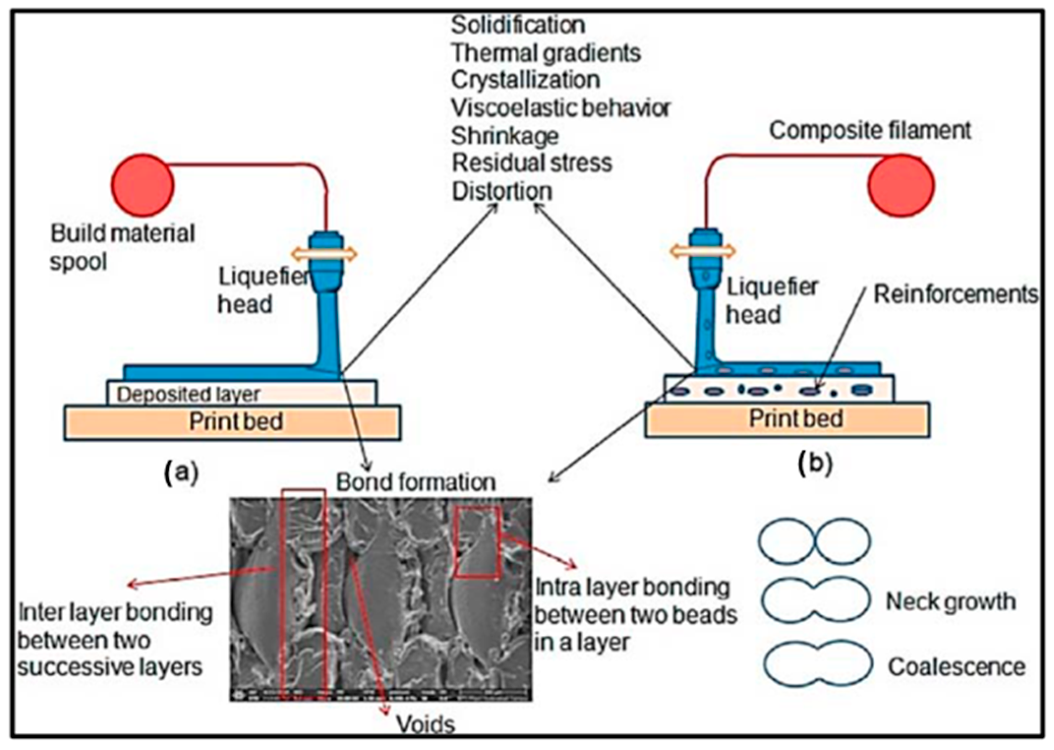
2. Challenges and Key Factors in the 3D Printing of Composites

Being a relatively new technology, several key aspects are worth studying. The results of the manufacturing process must respect the designated quality criteria [72].
In the context of an engineering assembly, the quality criteria relate first and foremost to the functional role. Alternatively, the aspect of the part is influenced by the technological parameters. Lastly, the process performance is also influenced, allowing competitiveness with conventional composites. The parameters’ influences are shown in Table 1. The slicing strategy enables a better coverage of the built volume, which is crucial for anisotropic structures like composites, resulting in an enhanced structural stability and deposed material in the designated stress areas. Voided volumes are inevitable in 3D printing due to the elemental deposition, resulting in a factor of embrittlement and a common cause of structural failure. The optimization of trajectories induces the continuity of fibers and their orientation, representing a key factor for the directional strength of the composite. The extrusion temperature leads the recrystallization process, resulting in dimensional deviations (warping) and induced residual stresses, thus making the component brittle. The nozzle diameter influences the fiber orientation and fiber volume content (proportional with strength) due to the flow of solid reinforcements into the molten matrix. The building plate temperature impacts the formation of the first layer and the interlaminar adhesion, leading to delamination failure. In less severe cases, the surface could be affected by wrinkles or sinkholes. The layer height directly influences the lead time of the process. Nevertheless, an increased layer height causes a coarser structure and a high-temperature gradient, which impacts the warping and residual stresses; the shrinkage may also cause the delamination of the consecutive layers, which can lead to the failure of the component and voids the formation. The aspect of the part could be affected when the layer height or the temperature is too high. Ultimately, the printing speed causes fibers to settle on a different orientation than expected due to a faster crystallization; indeed, some areas may cause voids. All in all, the combination of optimized parameters results in a performant process and component.

3. Finite Element Simulations of Additive Manufacturing Processes for Composites

The current section aims to assess the types of finite element analyses performed on the processes presented before, as shown in Table 2. The aim of these analyses is to optimize AM processes for composite structures, tuning the technological parameters and predicting defects, as presented in the prior section. The global AM process for polymers can be seen as a series of physical phenomena that are potentially modelled via the finite element method (FEM) [80] or the finite volume method (FVM) [81]. Considering the random orientation of the fibers and the computational capacity, composites are widely modelled using a representative volume element (RVE) [82].
The deposition process of AM composites can be divided into several areas of interest. The current section presents, via FEM or FVM, analytical models of the manufacturing phases in the technologies presented in Section 1, mainly CF/GF and thermoplastic and thermoset matrices. The phases of AM are categorized (Brenken et al., 2018) [36], as presented in Figure 4; the first area of interest is the nozzle, where the matrix undergoes a phase change. The solid fibers show a viscous flow into the matrix, resulting in fiber orientation. The unitary layer might be studied as a bonding between the current and previous raster, with the fibers having to flow on top due to the gravitational effect. Lastly, the solidification of the layer is studied with a focus on shrinkage (warping and residual stresses), the thermal trace, and, ultimately, the elastic behavior of the structure.

3.1. Pre-Processing (Slicing and Trajectory) Optimization

Composite specimens are mainly formed on a 0° fiber orientation, though AM enables one to develop various deposition strategies, presenting opportunities for design alternatives via the use of techniques such as topology optimization (mass/stiffness-oriented redesign). The case of short carbon fibers (SCF) and the polyethylene terephthalate glycol (PETG) matrix (Shafighfard et al., 2021) [83], is based on a rectangular plate with a hole in the middle, as used in a common stress concentrator test, as shown in Figure 5. The method was developed using the Halpin–Tsai homogenization method for design optimization (LSC), where the boundaries of the raster are defined, see Figure 5a, and the different orientation areas are emphasized, as seen in Figure 5b.
The difference with unidirectional strands lies in their ability to prevent interruptions in the path near the stress concentrator [84]. The conventional building strategy (0°), as seen in Figure 6a, shows higher peak values around the stress concentrator as the load increases (10 MPa, 12.5 MPa, respectively; 15 MPa), whereas the curvilinear optimized path, presented in Figure 6b, presents lower values with a relatively evenly distributed strain due to the stress occurring along a continuous path, which, in other areas, unloads in a normal direction, as in the case of 0°, where tangential inter-fiber unloading can be observed.
Further investigation has demonstrated continuous deposition paths, as one can see in Figure 7, which form the basis of the concept of a flow over a cylinder. The idea behind this concept originates from path definitions following curvilinear directions, as inspired by natural structures (such as branches on a tree trunk). In utilizing this method, the material avoids any interruptions in the deposition around the stress concentrator, even though the geometry is slightly altered.
The path optimization becomes of more relevance in the case of continuous fibers, which can assure the continuity of the fibers. The path topology optimization, in the case of continuous carbon fibers (CCF) and PA, (Chen et al., 2023) [85] develops models where the initial volume of the part was reduced, as visible in Figure 8.
Stresses were observed when the material was subjected to 1% effective strains, particularly those occurring in the intersectional areas for CCF-PA, as shown in Figure 9b, as the rest of the material was less vulnerable. On the contrary, for PA, the strain is distributed throughout the whole structure. This may lead to a decrease in the fiber content, eventually leading to a cost optimization.
Due to the complex shapes, where continuous fibers can become difficult to lay on the trajectories and fill the surfaces, a combination of SCF/PA and CCF/PA (Chen et al., 2021) [86] is used toto manufacture a complex component. The application starts as a fixed-end plate featuring a hole, as one may see in Figure 10a. Following the topology optimization, the filling strategy was performed to prioritize continuous fiber paths (without interruptions), as one can see via the blue paths in Figure 10b; in the areas where continuous path generation was achieved, a SCF-PA composite filament was employed (as indicated by the red contours in Figure 10b).
A comparison of the levels of stiffness between pure PA, SCF-PA, and CCF-PA is illustrated in Figure 11a, with the levels being almost two times higher for SCF, and twelve times higher for CCF. The peak load is five times higher for SCF, and sixteen times higher for CCF, as shown in Figure 11b.
The presentation of the path optimization of thermoset composites (DIW) (Qian et al., 2021) [87] is significant. It was built a porous SCF/Poly-carbosilane catalyst structure for the production of hydrogen via reforming methanol steam for fuel cells, as one can see in Figure 12a. It is meshed so the channels can be more refined, as shown in Figure 12b.
The scope of this optimization mainly concerns the reformation of the methanol steams process, with the aim of slowing the flow of the methanol, as seen in Figure 13a. On the other hand, the hydrogen concentration is the highest at the end of the channels, as one can see in Figure 13b. This optimization leads to a better overall efficiency of the process, as well as the construction of small reactors for applications such as hydrogen fuel cells to be used in vehicles, which can be fueled using methanol, making storage easier and less hazardous than in liquid hydrogen tanks.

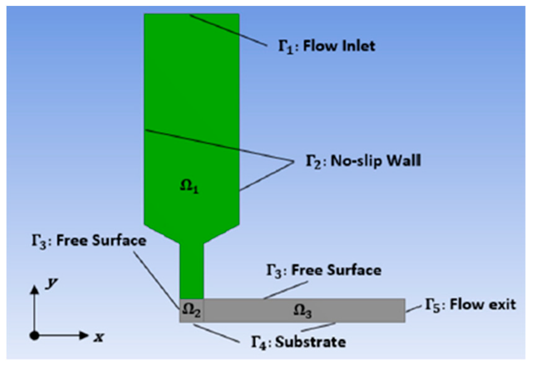
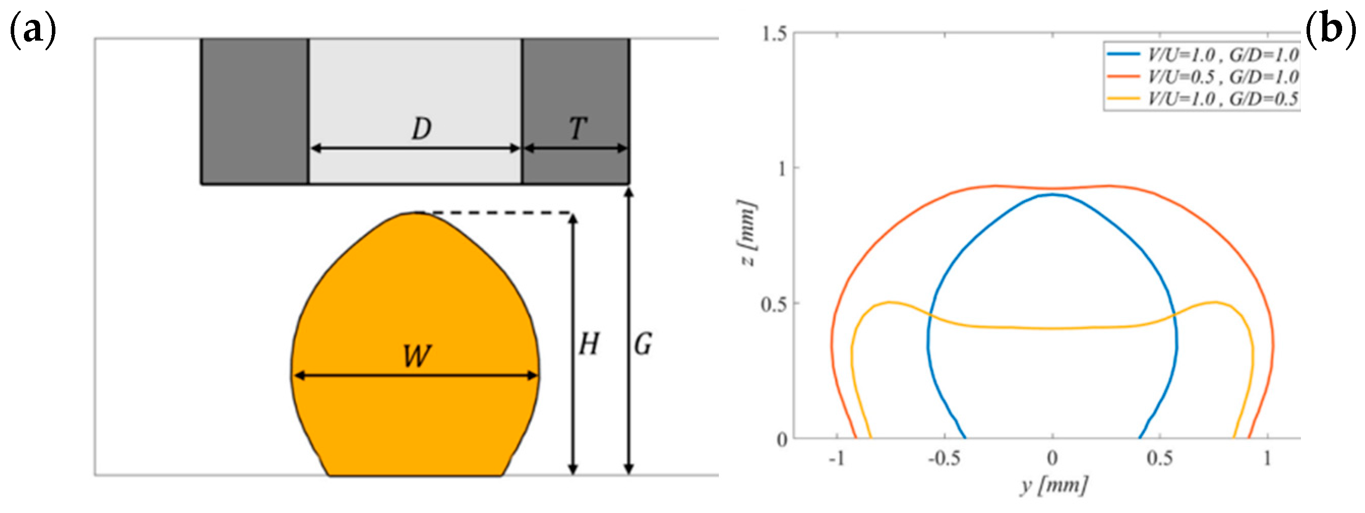
3.2. Computational Fluid Dynamics of Additive Maufacturing Composites

Computational fluid dynamics represent the differential numerical modelling of the equations of energy transfer in a fluid tridimensional medium (Navier-Stocks) (Date Anil W 2005; Hu 2012) [88,89]. Xu et al. made a categorization of CFD domains in the context of 3D-printed composites (Xu et al., 2023) [90]. The process starts with a multi-phase flow (solid/liquid) into the nozzle, as shown in Figure 14a. In the extrusion process, the fibers are flowed into the molten matrix, resulting the fiber orientation, whereas, in the continuous fiber composites, this will result in fiber deformation, as seen in Figure 14b. Following the phase transformation (liquid/solid), the dimensional deflection is simulated until convergence is achieved.

3.3. Melting Simulation of Additive Maufacturing Composites

A multi-phase transformation FVM model of PEEK AM (Wang et al., 2019) [91], which proved important for applications that entailed high temperatures/high strength (aerospace and defense applications) and biocompatibility. This model employed Ansys Fluent, utilizing the Cross-WLF viscosity law [92]. The geometry of the multi-stepped printing head demonstrates the gradient heating of the filament from the chamber temperature (68 °C) to the extrusion temperature within the nozzle (380 °C), and the filament displays convex-shape heating, beginning in the walls, as seen in Figure 15a. Before the extrusion, the filament starts the phase transformation from the heated walls, continuing to the tip of the nozzle, as seen Figure 15b. The multi-phase transformation temperature gradient is shown in Figure 15c, with a decreased viscosity of 14 Pa·s (liquid phase).

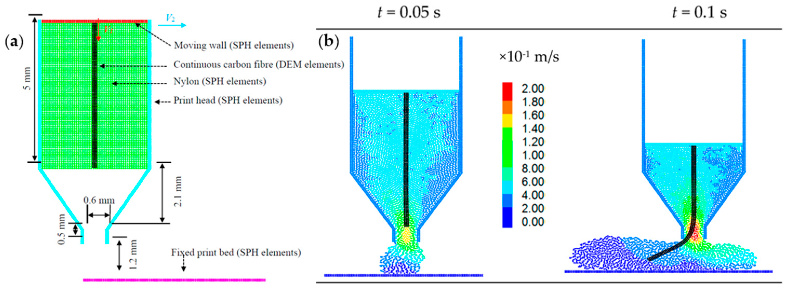
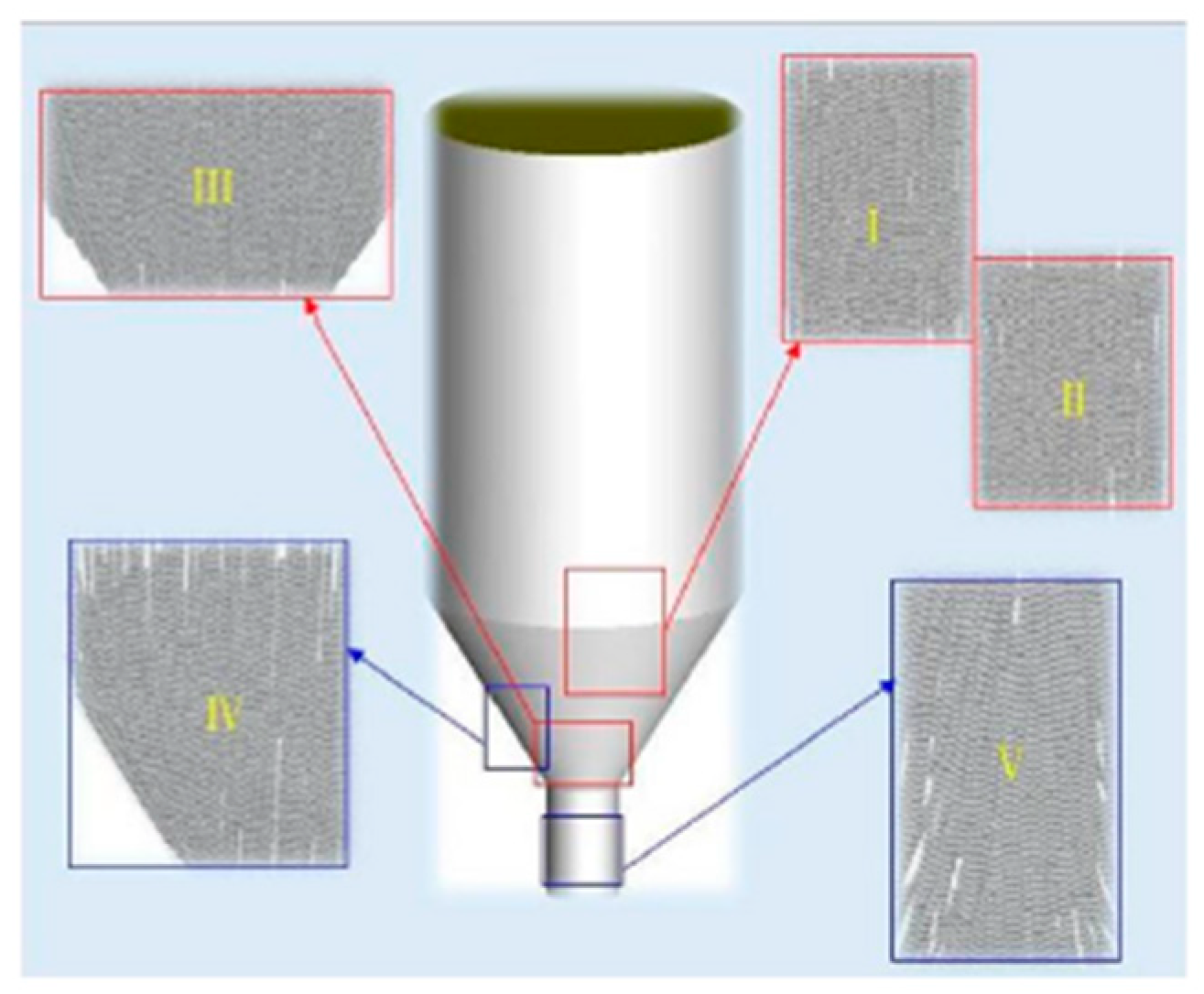
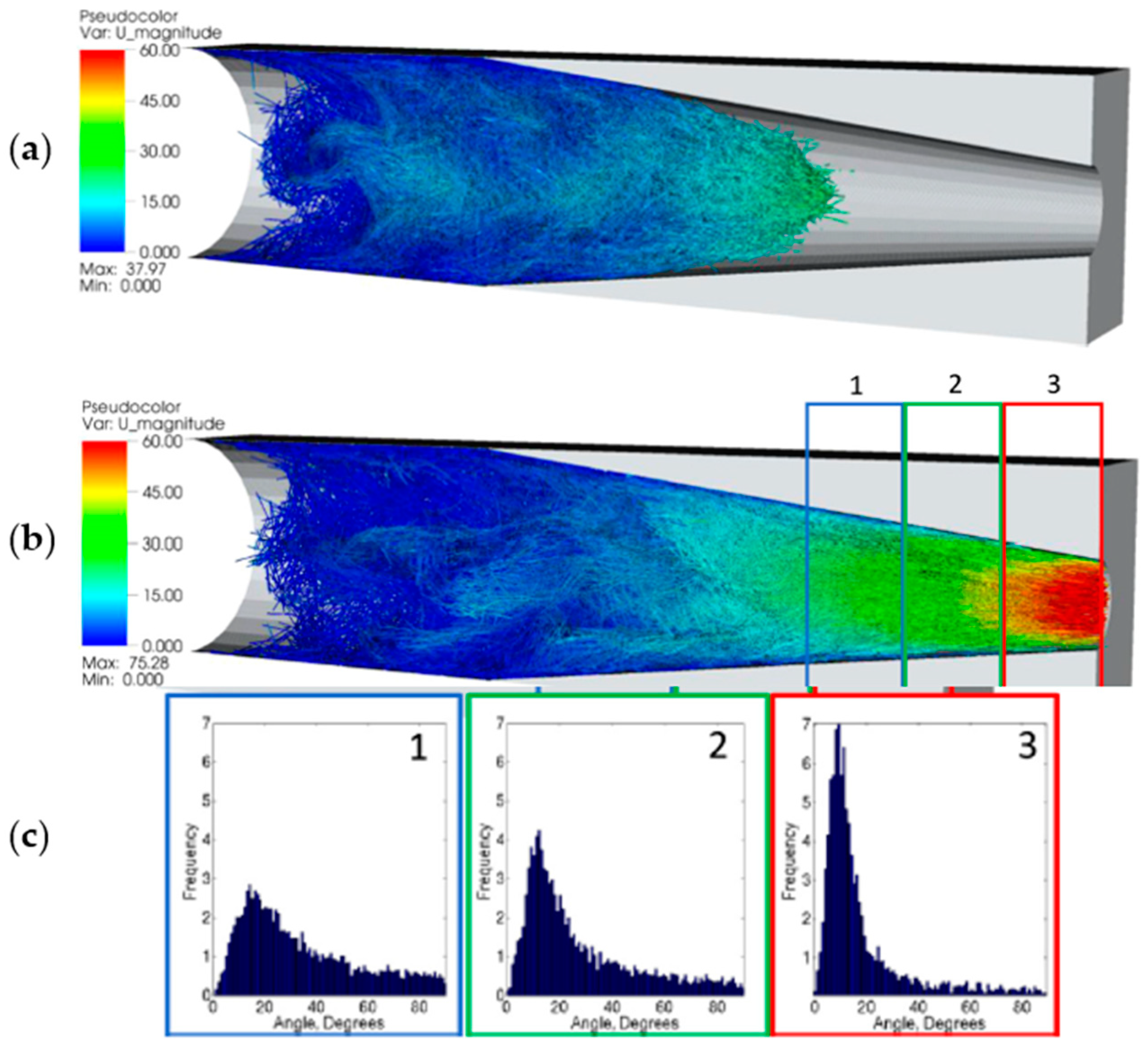
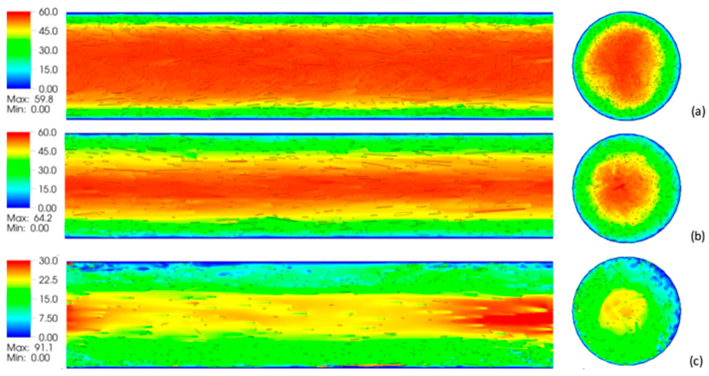
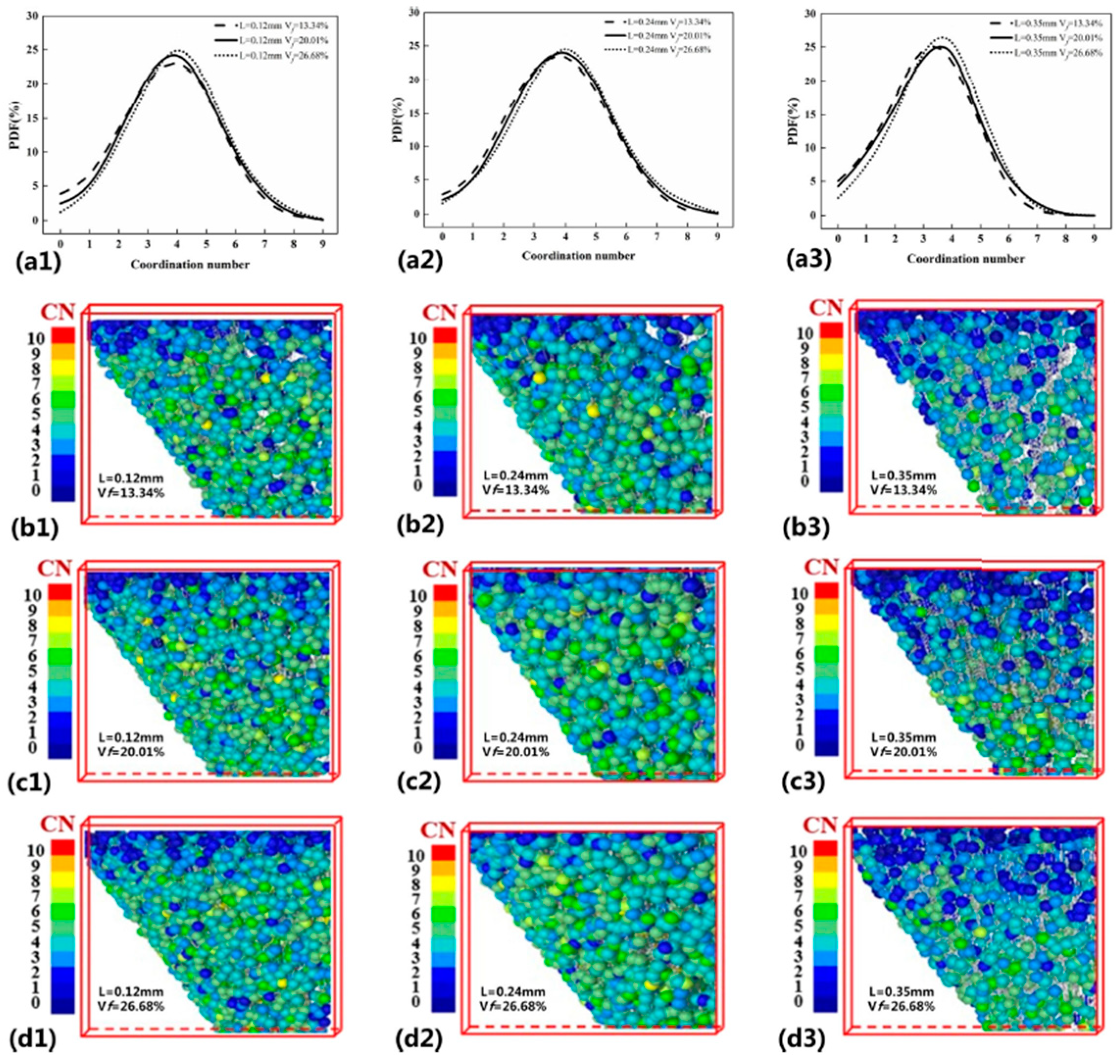
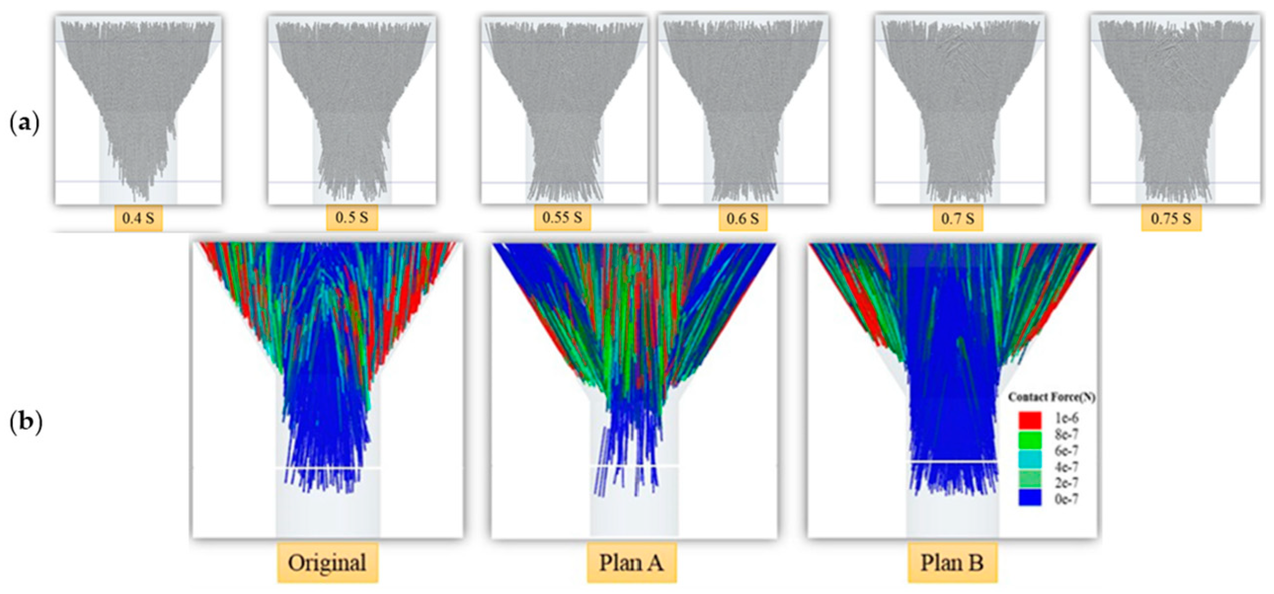
3.4. In-Nozzle Flow for Additive Manufacturing Composites (Fiber Orientation)

The second phenomenon of interest in CFD concerns the flow dynamics. In this case, an isothermal model of short-glass fibers in the molten ABS suspension (Yang et al., 2017) [93] who utilized the SPH-DEM (smoothed particle hydrodynamics–discrete element modelling) approach [94,95]. This model consists of solid short fiber (DEM) elements and fully fluid ABS DEM elements, as shown Figure 16a, where the moving wall pushes the composite through the nozzle at a certain flow rate. The transient model presented in Figure 16b depicts the flow velocities at two separate moments: firstly, when the first particles arrive at the diameter reduction (nozzle), where the flow rate increases, and secondly, when the particles passed through nozzles demonstrate free flow on the deposition bed, thus slowing the flow rate; however, the rate in the nozzle increases due to the gravity of the particles to be extruded.
Concerning continuous fibers, a SPH-DEM model (Yang et al., 2017) [93] with similar approach to the case of short fibers, as seen in Figure 17a. The in-situ impregnation of continuous CF-Nylon is simplified due to the rigidity of the center. The flow simulation, visible in Figure 17b, presents a continuous carbon fiber flow with a high-speed flow velocity under the fiber, which can be attributed to the diameter reduction, as well as the pushing and higher viscosity of the solid fiber, which is continuously fed. The laying of the continuous fiber shows a non-linear placement that may eventually influence the material’s isotropy.
In the continuous fiber, stresses can be withstood due to the pressure in the area opposite to the deposition direction, as one may see in Figure 18; these stresses can have values up to 450 MPa, which, in some cases, may lead to fiber breakage.
The flow of the thermoset resin and short carbon fibers by DIW (Kanarska et al., 2019) [96], is inspired by the Low Mach Code with Particle Transport (LMC-PT) algorithm, based on the Distributed Large Multiplier (DLM) technique found in the SAMRAI software v. 4.3.0. The suspension of fibers into the resin was modeled after RVE. The suspension flow was simulated in the transient domain with a constant increase in viscosity as the diameter diminished, as seen in Figure 19a,b. The first section shows a relatively even fiber dispersion over the angle, with a small peak around 20°. The tendency in the second area is similar, with peaks between 0° and 20°; however, in the third part (close to the extrusion area), most fibers are oriented around 10°, as shown in Figure 19c. This results in the control of the directional behavior of the resulting composite.
The cylindrical nozzle geometry emphasizes the differences between short fibers of different diameters, as shown in Figure 20. In the first case (Figure 20a), there are 0.15 mm diameter carbon fibers. The flow is relatively constant in the central area, and decreases near the walls due to the adhesion. The orientation is more dispersed, which is due to the lower viscosity of the resulting composite material. As the fiber diameter increases, the flowing speed decreases, and the fiber orientation is closer to 0° (Figure 20b,c).

3.5. Extrusion Defects Simulation

A specific defect of composite AM, both in terms of thermoplastic and thermoset, is the clogging of the nozzle, which occurs due to the higher viscosity caused by the solid fibers in the nozzle. Due to this phenomenon, the fibers will adhere to the extruder’s walls and the composite material will have less fiber volume content, thus resulting in less mechanical strength. Another downside is the turbulent flow that will occur inside the nozzle, which can lead to an unpredictable fiber orientation. This will affect the directional strength of the composite structure. Lastly, the process performance is affected by the frequency of nozzle changes resulting from abrasion and the increased failure rate due to any clogging that occurs during printing [77,79].
The FVM model (Zhang et al., 2021) [97] of nozzle extrusion (SCF-PA) via the SPH-DEM method (CF as DEM particles, SPH matrix) was performed using Ansys Fluent. During this process, various reinforcement volume fractions (Vf) were considered, including 13.34%, 20.01%, and 26.68%, as well as various raster widths (L), such as 0.12, 0.24, and 0.35 mm. The Figure 21 presents the filaments into the nozzle in different areas (I, II—beginning of diameter reduction, III—stabilization of extrusion diameter, IV—reduction to the extrusion diameter, V—extrusion area). The IV area of Figure 21, which is the most vulnerable area due to the diameter change. The initial results are coordination numbers (CN), which are a measure of the packing structure of the composite and the contact points between particles.
In all cases of raster widths, there is a Gaussian distribution of median CN with higher peaks (probability density function) for Vf = 26.68%, as seen Figure 22a; this is due to more solid particles being in contact. Alternatively, the variation of singular values for particles has been studied, as one can see in Figure 22b–d. The small particles represent the matrix, whereas the small cylinders represent the contact between the matrix and the solid particles; as the volume reduces, the CN grows due to the space reduction.
The flow analysis shown in Figure 23a emphasizes the construction of the fiber flow over time (bridging), where, initially, the front takes a convex shape (a laminar flow), and then the fibers tend to spread to the walls due to the adhesion of the fiber matrix. Ultimately, due to the feed rate, the process converges after 0.75% in a relatively constant tubular flow of the fibers, which is useful for the prediction of the fiber orientation during the process. The geometry of the nozzle influences the contact force of the composites at the wall of the nozzle in the IV area, as one may see in Figure 23b. In the conical area, the original design shows a high contact pressure, whereas, in the second design, the contact force is balanced. The last design shows a central constant contact force.

3.6. Deposition Simulation (First Layer Simulation for Thermoplastic Composites)

The following phenomenon studied includes the assessment of the elemental deposition trace and the fiber orientation relative to the direction of deposition, both in the cases of thermoplastic and thermoset matrix AM composites. The deposition of the first layer of the 3D-printed structure was studied. The numerical method can be defined as a series of boundary conditions, as seen in Figure 24. In general, the nozzle is considered a slip-free heating source for simplification. The first layer in contact with the printing bed (temperature regulated) is reduced to a constant height and length area.
In the case of SCF, the fluid flow in the first layer FVM model (Kermani et al., 2023) [99] was developed in COMSOL Multiphysics, using the Advani–Tucker model [100], and comparing Newtonian and Carreau viscosity models [101]. Reinforcement fibers are considered directional vectors, and the fiber orientation model is user defined (Coefficient PDE model). The short fibers in the nozzle are considered to be randomly oriented.
Therefore, it can be remarked in Figure 25A that the orientation tensor of the fibers shifts abruptly in an area of interference between a 90° direction change and the deposed layer. The orientation of SCF can be observed in Figure 25B. The core shows the gradients concentrically, ranging from 40% to 0%, indicating the probability of the desired outcome to be higher than at the center of gravity. The outer layers show an almost certain orientation of 0°, On the transversal cross-section, as seen in Figure 25C, the gradual adhesion to the printing bed can be seen, with a core of 0–20% around the deposition orientation, whereas the outer surface that has been subjected to shrinking almost certainly displays the predicted direction.
The raster cross-section displays a flat base attached to the printing bed and a bell-shaped path trace, as seen in Figure 26. The strand profile tends to increase in height as the distance from the nozzle is made smaller, due to the compression reaction. In time, it could be remarked that, after 0.5 s, the strand height tends to display a constant profile. The experimental setup is presented in Figure 26a. This is defined by G (the gap between the nozzle and the printing bed) and D (the diameter of the nozzle). A reduced diameter nozzle forms a more rectangular strand, where the material in the middle tends to migrate to the corners of the strand due to the compression induced by the following strand, as visible in the yellow contour presented in Figure 26b. The third strand shape corresponds to the speed (V) to feed rate (U) ratio being decreased to 0.5, as seen in the red path in Figure 26b, resulting in a higher volume, an enlarged base, and an increased contact surface with the adjacent raster and the printing bed.
The difference between the first row of images in Figure 27 and the second is the probability of short fiber orientation on the X-axis (as discussed in the previous section) and in the Y-direction, resulting in a fiber orientation of 50% in the y-axis direction of the core. This means that the material can be considered orthotropic with a probability of 60%. The lower G/D shows a superior fiber orientation stability, with a relatively smaller “core”-oriented volume, as one can see in Figure 27C,D.
As discussed in terms of the single direction extrusion process, the more practical case of in-plane deposition and direction change has been analyzed (Zhang et al., 2023) [102]. The numerical model is a non-linear transient for CCF-PA, developed in ABAQUS. The normal strain, see Figure 28a, is the measure of fiber deformation, where the direction changes in trajectories at 30° show an increased compression at the angle change and shows tension at the deposition layer. The shear stress, see Figure 28b, shows the fiber’s tendency to break, whereas the angled raster shows a significant risk of breakage. The contact pressure (nozzle-filament), see Figure 28c, has a similar profile due to the change of direction, where red circle 1 area is compressed in the nozzle, and the red circle 2 area is elongated, and the deposed raster tends to bond less to the previous material.
The effect of normal stress when the angle is changing is shown in Figure 29, where, for the interval between 15–30°, the printing width and strain is constant in the changing direction, whereas, for angles between 45–75°, the width increases due to the high stress, and a bending of the inner fiber is represented by the ellipses dotted area in Figure 29. In the extreme case of 90°, the width becomes unrealistic, corresponding to a break into the fibers.
The variation of the curvature radii effects is shown in Figure 30. The shear stress is reduced when R = 20 mm, whereas, for radii of 5–10 mm, the wrinkling phenomenon occurs (dotted ellipse area), as the stress area increases in the turning area. In the case where R = 2.5 mm, the shear appears in both external and internal areas, which signalizes a potential fiber breakage, emphasized in the turning area as the dotted contour. The variation of the raster width displays an increase in the shear strain with the augmentation of the bundle, which then increases the possibility of fiber misalignment and breakage.
The previous model was developed for planar paths and curvilinear printing paths (K. Zhang et al., 2023) [103]. The model is a meso-scale RVE, where the volume of continuous filaments is visible in the cube (Figure 31) and the filaments oriented along the extrusion direction. There were two nozzles in this analysis as follows: a geometry cylindrical M-shaped nozzle (planar deposition), and a rotational R-shaped nozzle (multi-axis deposition). Firstly, the raster is compressed by the nozzle tip. The second phase includes the nozzle moving in a single linear direction, preceding the curvilinear trajectory of the nozzle (only planar for the M-shaped and Z-axis increments for the R-shape).
The first step is rectilinear deposition (highlighted on the dotted contour), wherein transverse normal plastic strain occurs due to the compression of the nozzle, as shown in Figure 32. This indicates an uneven but smaller amplitude (maximum 0.19) distribution for the M-nozzle, as visible in Figure 32a, which is understandable due to the higher levels of compression resulting from the higher bending transition, whereas, in the case of the R-shaped nozzle, a wider angle (135°) assures a constant but higher residual strain (maximum 0.4), as one can see in Figure 32b. The bottom surfaces show the same tendency, with discontinuity occurring for the M-shaped nozzle due to the non-uniform contact pressure. In this way, a higher value means a higher warping tendency, but also a constant raster with better fiber alignment.
In terms of the transverse shear strain (the measure of shearing fiber occurrences), it can be observed in Figure 33a that the more curvature in the transition area in the case of M-nozzle shows a higher concentration, with a 0.29 relative strain, and a punctual compression area (−0.9), displaying variations along the way, which can then cause fiber slitting and out-of-plane buckling. The R-nozzle displays a relatively gradual deposition area, where the material suffers a relative compression of −0.6, as one can see in Figure 33b.
The second step is printing on a circular path using a constant 2.5 mm curvature for both geometries. The logarithmic strain was used as a measure to assess the filament torsion during the printing process. The small values indicate no torsion filaments, a phenomenon that increases before deposition in the M-nozzle across the entire filament, as one can see in Figure 34a, whereas, in the R-nozzle, the strain only manifests on the outer surface, as one can see in Figure 34b in the transversal section.
The curvilinear direction change (R = 10 mm between the trajectories) can be seen from above in Figure 35. The plastic strain tends to be smaller but inconstant (compression from the nozzle) for the planar M-shaped nozzle, with a gradual filament twisting of 45–60°; the fibers have a tendency to irregularly distribute in the middle of the directional change, making the structure with the M-shaped nozzle more vulnerable to breakage, as seen in Figure 35a. The R-shaped nozzle path, see Figure 35b, results in a more strained structure, which can be compensated via shrinkage, but this results in a regular distribution along the path, which results in a better performance of the resulting composite.
A tighter radial directional change (R = 2.5 mm) analysis was performed. The M-nozzle shows a significant strain at the 60–75° area (was occurred earlier and at an increased level when compared with the previous case), even if the fiber has a gradual tendency to twist (see Figure 36a). On the other hand, the R-nozzle demonstrated steep twisting around the 90° area (see Figure 36b), where the fiber has a sudden orientational change, and sudden folding occurs at 135°; this means that the curvature is considered too tight for this nozzle configuration.
The last step is performed on the frictional contact point between the filament and the nozzle in the dotted contour area, as seen in Figure 37, in a non-planar deposition, where the M-shaped nozzle displays a positive/negative split line at the middle when printing. The structure becomes widely compressed following this, as visible in Figure 37a. However, the R-shaped nozzle maintains a relatively constant split line throughout the process, which reduces the twisting and optimizes the fiber orientation along the deposition direction, as presented in Figure 37b.

3.7. Solidification of 3D-Printed Composites (Residual Stress and Dimensional Precision)

The solidification process is worth evaluating in terms of the temperature field distribution, the induced thermal deformation, or the residual stresses within the printed part. Also, reconstituting the material deposition is an FEA case in itself, which presents particularities for composite materials due to the resulting directional properties.
The case of short wood fibers and PLA is a thermo-mechanical numerical model of the deposition (Moryanova et al., 2023) [104], which was completed in parallel with the experimental model of the 20 × 20 × 20 mm cubic composite specimen. The first aspect studied was the warping of the 3D-printed composite with different layer heights (0.15 mm and 0.25 mm), as can be seen in Figure 38a. For a layer of 0.5 mm, the warping tendency is higher on the middle-top layers towards the barrier of 0.5 mm, showing a gradual decrease towards the building plate. The lower height (0.15 mm) displays an improved warping tendency, with the middle layers being the most deformed around 0.35–0.4 mm. The experimental results show coarser top edges with deposition defects for layers at higher heights, as visible in Figure 38b.
In the cooling process, deformation results in stresses due to the movement of the particles, adhesion, and the phase change of the matrix. As one can see in Figure 39, the lower the extrusion temperature, the lower the stress levels. The areas where the residual stresses are highest are on the boundaries of the part, where lower heights result in a thinner boundary stress of 30 MPa, whereas, for the increased layer heights, the boundary stresses meet 45 MPa on the lower area (0.2 mm), as well as on all the 0.25 mm boundaries of the cube.
Lastly, the temperature field distribution was studied and found to be uniformly distributed throughout the printed cube (3 s after finishing the process) for all layer heights, as one can see in Figure 40. The boundary layers cool at a higher rate, resulting in, as remarked in the previous sections, more defects, and coarser structures.
The numerical model of deposition (Chnatios et al., 2023) [105] is a thermo-mechanical coupled simulation for CCF-PEEK. The magnitude of warping caused by the variation of process parameters was demonstrated. Due to the computational difficulty, a single-layer deflection was calculated, and it was found that warping increased continuously as the manufactured thickness grew; this was due to the reheating of the previously manufactured areas. The high-temperature PEEK composites leave a thermal trace, as one may notice in Figure 41. The higher the thickness, the more pronounced the thermal footprint; Figure 41a shows a lower strain than that shown in Figure 41b. The printing bed temperature (150 °C) will cause additional thermal deflection following printing when cooling to room temperature.
As the heat transfer exists between the previously deposed raster and the current layer, the deflection grows with the number of layers (Z-height), as well as with the width of the part (Y-axis), as one can see in Figure 42, where a change from 2.02 µm (layer 3, Figure 42a,b) to 3.8 µm (layer 5, Figure 42c,d) can be seen. The deflection can be observed on the edges of the raster, where the cooling occurs last, causing the material to warp (free surface on the edges). This is considered the most important factor in warping, as it is quite unavoidable in most applications.
The printing bed temperature can limit the warping, reducing from 9.048 µm for a standard temperature (150 °C, Figure 43b), to the insignificantly lower 0.904 µm (155 °C, Figure 43c), and again to 0.891 µm (160 °C, Figure 43d). The deflection has a reversed tendency for lower temperatures, which is even more pronounced at 0.917 µm (145 °C, Figure 43a). This is a result of a lower temperature variation between the raster and the printing bed.
In addition, the printing temperature variation was studied, as seen in Figure 44. The more significant warping was 1.52 µm (390 °C, Figure 44a), constantly decreasing to 1.425 µm (400 °C, Figure 44b) or to 1.323 µm (410 °C, Figure 44c). The standard temperature (420 °C, Figure 44d) shows the smallest deflection of 1.21 µm. This is understandable due to the viscosity variation of PEEK when suspended with CF.
The printing speed influences the warping, as shown in Figure 45. The lowest speed (υ = 1 mm/s, Figure 45a) shows the smallest deflection of 1.172 µm. The increase observed in the speed results in a 1.21 µm deflection (Figure 45b,c) stabilized in the range of υ = 3–5 mm/s. Exceeding the standard speed results (υ = 3–5 mm/s, Figure 45c) following a steep increase in deflection to 1.362 µm can be explained via the faster deposition, higher heat transfer over time, and the optimal speed being a compromise between the precision and manufacturing time.

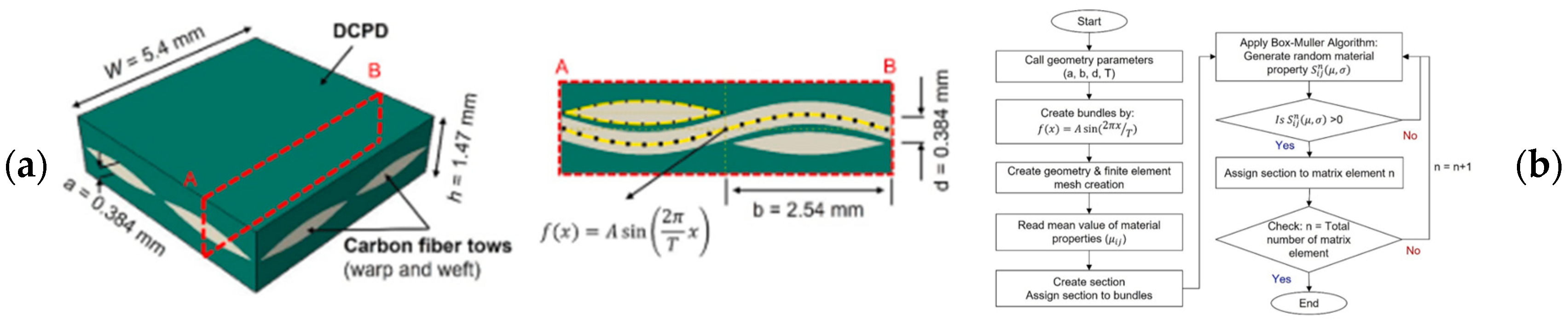
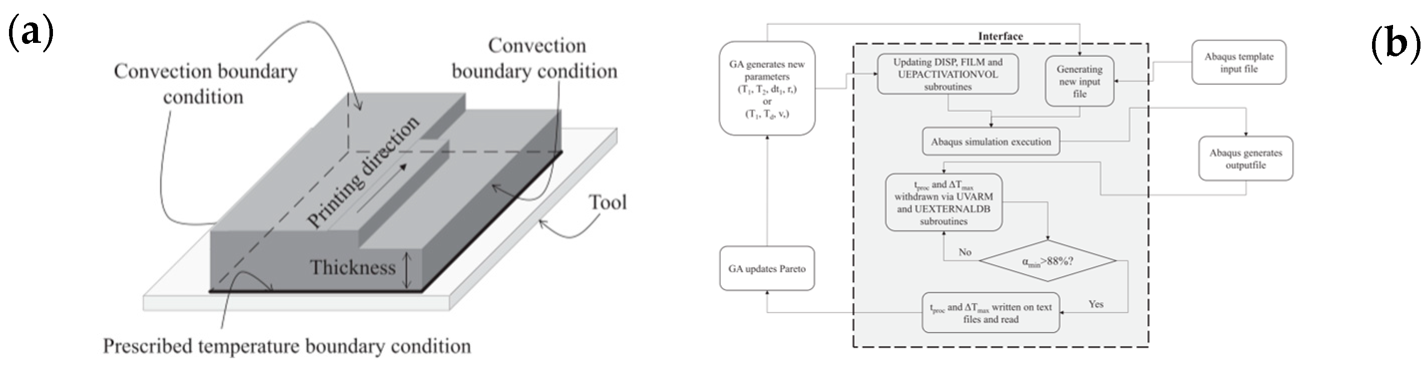
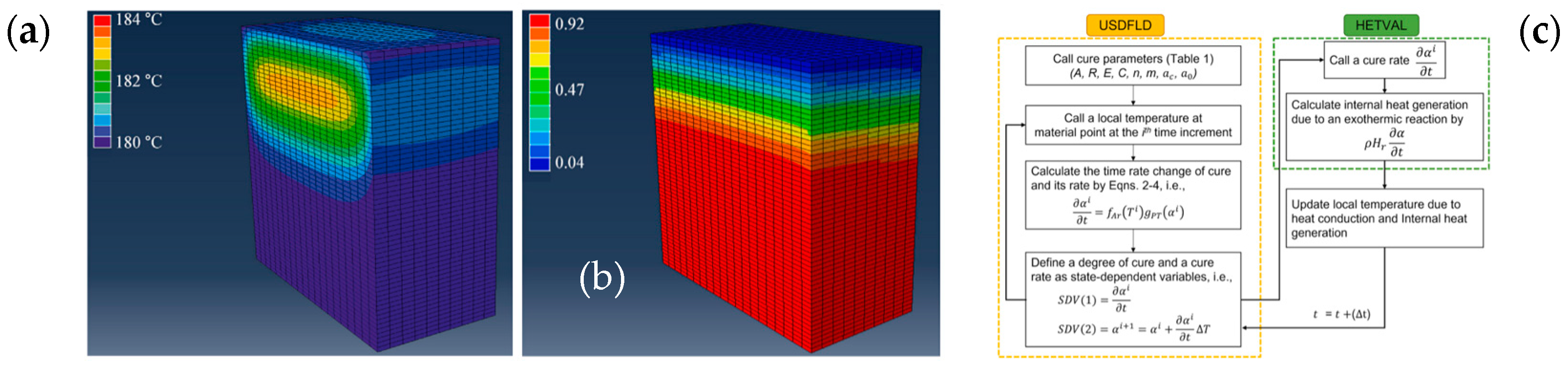
3.8. Solidification of 3D-Printed Thermoset Composites

In the case of thermoset composites, the solidification process (curing) is performed via several sources of external energy or via the chemistry of the matrix. The thermal polymerization of thermoset matrix composites (Struzziero et al., 2023) [106], is focused on Epoxy-CF-based composites. The model was a 2D deposition layer, as seen in Figure 46a, where a convection surface can be found at the boundary of the deposed layer. This was developed in ABAQUS, utilizing a C++ general algorithm for the material properties based on the logic shown in Figure 46b.
The temperature map of the curing process is shown in Figure 47a, highlighting the tendency of curing around 183 °C, spreading concentrically throughout the raster. The model was developed in ABAQUS, using USDVLD to calculate the curing state in differential time HEVAL subroutines for the heat generated via exothermic curing, following the conditions displayed in Figure 47b. Based on the algorithm earlier described, the state of curing is shown in Figure 47c, where the previously deposed layers display a curing state of 89–92%. It can be observed that the material consumed most of its activation energy, maintaining a constant curing rate during the process, and thus guaranteeing a constant thickness.
A prospective material development encompasses the usage of frontal polymerization thermoset resin for eliminating the need of molds and, especially, of post-processing treatments. The model for the state of curing for frontal polymerization (Sharifi et al., 2023) [107], is focused on continuous carbon fiber PDCPD resin (promising improved impact and corrosion resistance) as used on RVE, as shown in Figure 48a, in 3D and as cross-section of red-dotted contour. The stochastic material is defined via a routine in Python, as described in Figure 48b. The RVE is defined as a bundle equation creation. By applying the Box–Muller algorithm [108], the matrix is given random properties, respecting the standard deviation from the mean actual values of the characteristics.
Three types of material configurations were created for this simulation. The deterministic material is shown in Figure 49a with no voids. The second material configuration is stochastic Figure 49b, where the spatial distribution of the properties is randomly generated in different color elements, which is more suited for liquid resin that is prone to impurities. The third model is the first configuration, with randomly distributed 3% voids (red elements) throughout the volume Figure 49c.
The state of curing commences on a normal direction of the printed composite, as one may see in Figure 50 in 3D, then in A-B cross-section. The cases consider various standard deviations from the mean cured properties (SD), where the curing occurs around the fibers. On the other hand, the fiber/matrix interface cures last (after 3 s), where the cure state decreases with the SD augmentation, converging at 100% for each SP following 5 s. The other case treated in Figure 50 is polymerization in the direction of printing, where the curing is slower around the fibers and in between the fibers, the maximum curing latency being for SD = 40% at 3 s.

3.9. Defect Simulations of Completed 3D-Printed Composites

The defects numerical model (Moryanova et al., 2023) [104], that are visible in the Figure 38b are revealed in detail in Figure 51. The first remarked defects are the splattering marks (cracks, holes, traces), caused by the difference in crystallization states during the cooling of the layers, which is due to the high extrusion temperature and the wood fibers in the resulting composite. Splatter traces of 0.5 mm magnitudes were observed both numerically and experimentally, as seen in Figure 51a. For a lower layer height, a more stable surface is visible in Figure 51b, which is due to a more uniform distribution of wood reinforcements (solid fibers are lighter than the matrix and flow above), and the similar size magnitudes of fibers and the PLA layer.
Along the traces, in increased layer heights (0.25 mm), both numerical simulations and experimental observations demonstrated pultrusion into the outer surface due to twisting of the material (see Figure 52a). The quality of the interlayer seams and the sinkholes can be observed in Figure 52b, resulting from the time difference of the material deposition time in the cooling process. Ultimately, at higher extrusion temperatures (220 °C), a failure of the first layer was observed, which was due to the molten matrix and the considerable deposed mass, as one can see in Figure 52c.

3.10. Void Formation Simulation

As seen in the previous section, the cross section of the deposed layer is widely influenced by the process parameters, meaning the internal structure depends on each path. The process simulation of SCF-PEEK (Fu et al., 2023) [109], is done using ABAQUS with user-defined material (UMAT) subroutines [110]. Micro-scale RVE with periodicity was applied, as seen in Figure 53. Unitary deposed element is represented as a matrix cube, 5% SCF (black elements), modelled as cylinders inside the RVE, whereas voids are introduced in random volumes (blue particles). The orientation of the layers is defined as per the picture below, resulting in the tensile specimen.
The crystallization is presented within the printed layers like intervals of 0–1 (ωc), PEEK being a semi-crystalline matrix. Firstly, the deposed element is completely uncrystallized, as seen in Figure 54a. The crystallization process begins at the margins, where the matrix starts to cool, as visible in Figure 54b. When changing direction, as is visible in Figure 54c,d, the areas adjacent to the previous layer diminish their solidification state due to the interfacial heat transfer. As the process continues, the layer returns to a complete solid state as the distance grows from the currently deposed raster Figure 54e–g, and as voids appear between the printing tracks. In the end, the transfer to the following layer results in an insignificant change within the previous raster, as shown in Figure 54h. Once the process is over, the crystallization process is completed to almost 100%, with the crystallization between trajectories being over 85% due to the irregular heat flux from the adjacent deposed raster. Overall, it was calculated that the porosity simulation showed a peak value of 14.29% without any post-processing treatment.
The macro-scale model for CCF-PA (Zhilyaev et al., 2022) [111], developed in ANSYS with user-defined routines, where the phase transition is a Nakamura algorithm [112], and the mechanical properties are assigned based on experimental activities, as they are temperature dependent. The primary drawback of the continuous fiber composites is the level of porosity, which is exacerbated by the upright printed surfaces on the complex geometry, resulting in the highest void volumes of 8–10% in the support areas and at the overhanging hole areas, as visible in Figure 55a. The base area was subjected to higher porosities at points of sharp directional changes, as one can see in Figure 55b. The cumulative defects from the cases presented above result in a maximum of 24.1%, as visible in Figure 55c.

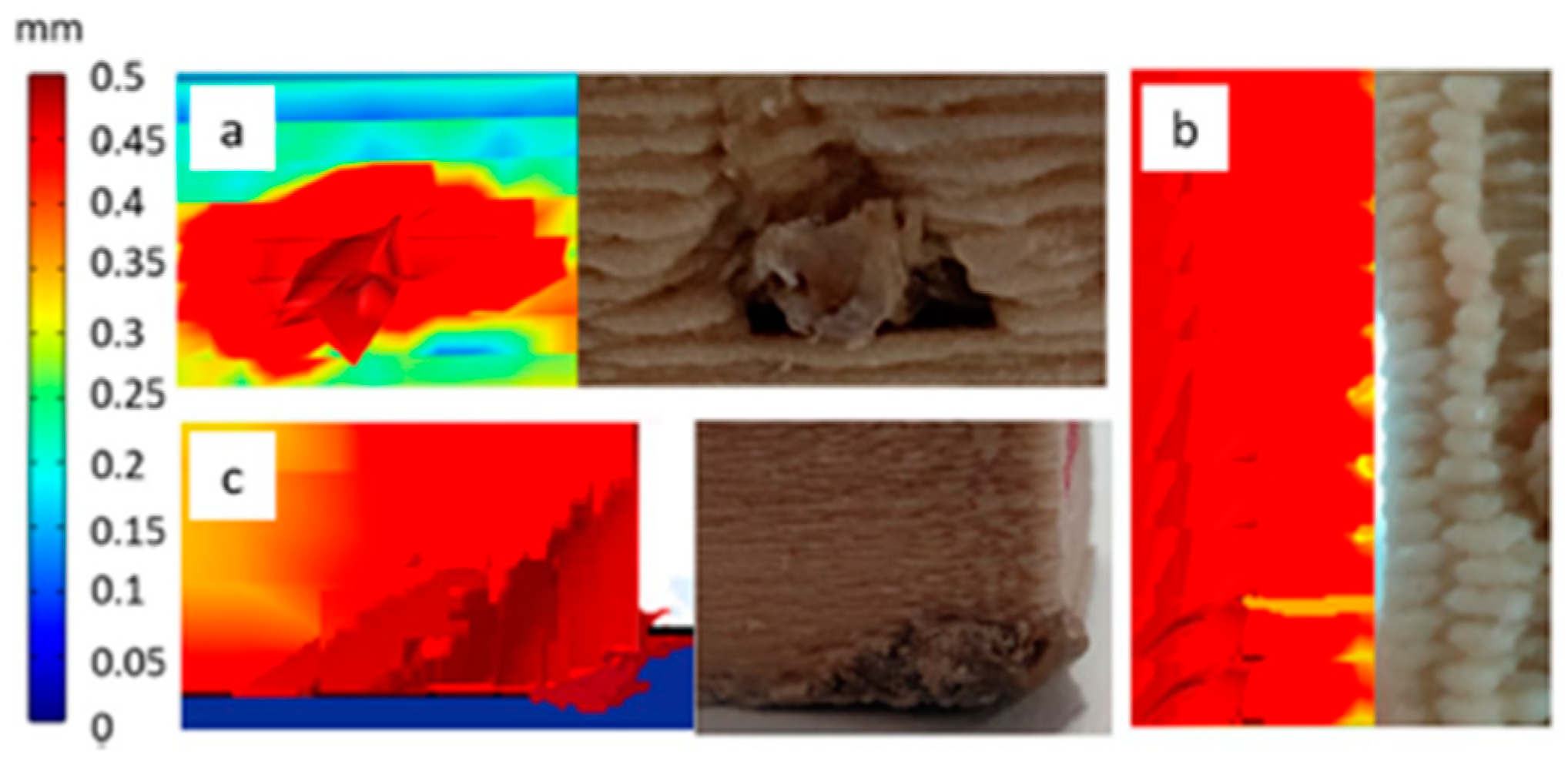
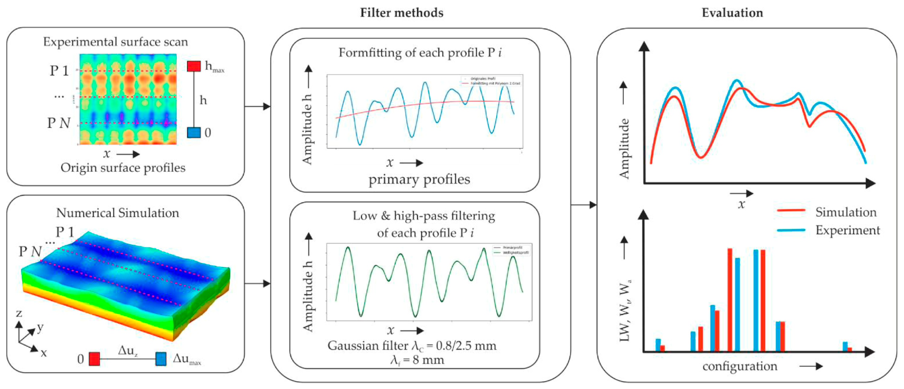
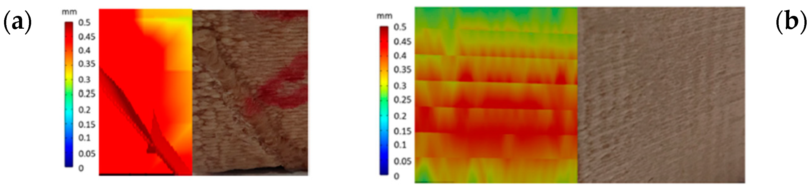
3.11. Surface Roughness Simulation

The surface roughness is important, especially for the aspect of the component. In addition, the contact area with other parts in the assembly is significant. Due to this, the roughness before any post-processing treatment is of great concern, especially in the case of thermoset matrix composites manufactured via AM, due to amorphous polymerization. The roughness simulation for continuous GF and bisphenol photosensitive (Lorenz et al., 2022) [113]. The model was developed in TexGen software 3.13.1, with experimental material properties. The model was developed for two directions, with mean profiles and extremum values, as shown in Figure 56. Plotted profiles for both experimental and simulation results can be found below.

3.12. Post-Processing Simulation

A post-processing treatment simulation (Grieder et al., 2022) [114], including hot pressing decreased the porosity from 20.28% to only 1.4% in the case of 240 °C/10 bars. The maximum void pressure was 1.6 MPa, as shown in Figure 57a, whereas the void content exists at the bottom of the bar Figure 57b, opposite the hot-pressing treatment. The fiber variation content was similar in profile to the porosity Figure 57c, ranging between 53–57%. Because it is used as a heat-resistant thermoplastic matrix, the elastic transverse modulus at heat deflection temperatures (175 °C) is studied and presented in Figure 57d, ranging between 3.84–6.47 MPa.

4. Conclusions

To conclude, the AM processes are diverse in terms of the material range and the nature of the reinforcement, as presented in Section 1. Due to their similarities with common AM technologies such as FDM or SLA, these have been developing at an accelerated pace over the last 5–10 years, and are showing strong potential to become widely used in composite manufacturing.
As the processes are in the development phase and their cost is a significant factor, especially for continuous fibers composites, addressing potential defects arising from the technologies they derive from, as well as specific composite defects, the digital twinning of the processes is highly desirable for industrial applications to remain competitive with their conventional counterparts. FEM represents a technique used to model the physical phenomena. In the case of AM composites, as presented in Section 2, there are several aspects to be considered, which are relevant if the process parameters are to be digitally optimized, involving many disciplines of finite elements.

Author Contributions

For this review concept, T.F.Z.; Resources T.F.Z.; Original and Draft Preparation: T.F.Z.; Review and Editing M.C.D.; Supervision: M.C.D. All authors have read and agreed to the published version of the manuscript.

Funding

This research received no external funding.

Data Availability Statement

Not applicable.

Conflicts of Interest

The authors declare no conflicts of interest.

References

  1. Gibson, I.; Rosen, D.; Stucker, B.; Khorasani, M. Introduction and Basic Principles. In Additive Manufacturing Technologies; Springer: Cham, Switzerland, 2021; pp. 1–19. [Google Scholar] [CrossRef]
  2. Associates, W. Wohlers Report 2022: 3D Printing and Additive Manufacturing Global State of the Industry; Wohlers Associates: Fort Collins, CO, USA, 2022. [Google Scholar]
  3. Huang, J.; Qin, Q.; Wang, J. A review of stereolithography: Processes and systems. Processes 2020, 8, 1138. [Google Scholar] [CrossRef]
  4. Hull, C.W. Apparatus for Production of Three-Dimensional Objects by Stereolithography. U.S. Patent 45,753,30A, 1 December 1977. [Google Scholar]
  5. Siemiński, P. Introduction to Fused Deposition Modeling. In Handbooks in Advanced Manufacturing; Elsevier: Amsterdam, The Netherlands, 2021; pp. 217–275. [Google Scholar] [CrossRef]
  6. Agarwal, R. Chapter 5—Additive manufacturing, Materials, technologies, and applications. In Additive Manufacturing: Advanced Materials and Design Techniques, 1st ed.; Pandey, P.M., Singh, N.K., Singh, Y., Eds.; CRC Press: Boca Raton, FL, USA, 2023; pp. 77–97. [Google Scholar]
  7. Yan, C.; Shi, Y.; Li, Z.; Wen, S.; Wei, Q. Selective Laser Sintering Additive Manufacturing Technology; Elsevier: New York, NY, USA, 2020. [Google Scholar] [CrossRef]
  8. The Evolution of SLS: New Technologies, Materials and Applications. Autonomous Manufacturing. 2021. Available online: https://amfg.ai/2020/01/21/the-evolution-of-sls-new-technologies-materials-and-applications/ (accessed on 12 January 2024).
  9. Prince, J.D. 3D Printing: An Industrial Revolution. J. Electron. Resour. Med. Libr. 2014, 11, 39–45. [Google Scholar] [CrossRef]
  10. Huang, Y.; Leu, M.C.; Mazumder, J.; Donmez, A. Additive manufacturing: Current state, future potential, gaps and needs, and recommendations. J. Manuf. Sci. Eng. Trans. ASME 2015, 137, 014001. [Google Scholar] [CrossRef]
  11. Sames, W.J.; List, F.A.; Pannala, S.; Dehoff, R.R.; Babu, S.S. The metallurgy and processing science of metal additive manufacturing. Int. Mater. Rev. 2016, 61, 315–360. [Google Scholar] [CrossRef]
  12. Joshi, S.C.; Sheikh, A.A. 3D printing in aerospace and its long-term sustainability. Virtual Phys. Prototyp. 2015, 10, 175–185. [Google Scholar] [CrossRef]
  13. Martinez, D.W.; Espino, M.T.; Cascolan, H.M.; Crisostomo, J.L.; Dizon, J.R.C. A Comprehensive Review on the Application of 3D Printing in the Aerospace Industry. Key Eng. Mater. 2022, 913, 27–34. [Google Scholar] [CrossRef]
  14. Nichols, M.R. How does the automotive industry benefit from 3D metal printing? Met. Powder Rep. 2019, 74, 257–258. [Google Scholar] [CrossRef]
  15. Rajak, D.K.; Pagar, D.D.; Behera, A.; Menezes, P.L. Role of Composite Materials in Automotive Sector: Potential Applications. In Advances in Engine Tribology; Kumar, V., Agarwal, A.K., Jena, A., Upadhyay, R.K., Eds.; Springer: Singapore, 2022; pp. 193–217. [Google Scholar] [CrossRef]
  16. Yan, Q.; Dong, H.; Su, J.; Han, J.; Song, B.; Wei, Q.; Shi, Y. A Review of 3D Printing Technology for Medical Applications. Engineering 2018, 4, 729–742. [Google Scholar] [CrossRef]
  17. Aimar, A.; Palermo, A.; Innocenti, B. The Role of 3D Printing in Medical Applications: A State of the Art. J. Healthc. Eng. 2019, 2019, 5340616. [Google Scholar] [CrossRef]
  18. Nagarajan, B.; Hu, Z.; Song, X.; Zhai, W.; Wei, J. Development of Micro Selective Laser Melting: The State of the Art and Future Perspectives. Engineering 2019, 5, 702–720. [Google Scholar] [CrossRef]
  19. Saengchairat, N.; Tran, T.; Chua, C.K. A review: Additive manufacturing for active electronic components. Virtual Phys. Prototyp. 2017, 12, 31–46. [Google Scholar] [CrossRef]
  20. Inkwood Research. Global 3D Printing Market Growth_Global Opportunities. 2023. Available online: https://inkwoodresearch.com/reports/3d-printing-market/ (accessed on 12 January 2024).
  21. Statista. Global 3D Printing Industry Market Size. 2021. Available online: https://www.statista.com/statistics/315386/global-market-for-3d-printers/ (accessed on 12 January 2024).
  22. Report Linker. Additive Manufacturing Global Market Report 2023. 2023. Available online: https://www.globenewswire.com/news-release/2023/06/21/2692058/0/en/Additive-Manufacturing-Global-Market-Report-2023.html (accessed on 12 January 2024).
  23. Zhong, W.; Li, F.; Zhang, Z.; Song, L.; Li, Z. Short Fiber Reinforced Composites for Fused Deposition Modeling. Mater. Sci. Eng. A 2001, 301, 125–130. [Google Scholar] [CrossRef]
  24. Shofner, M.L.; Lozano, K.; Rodríguez-Macías, F.J.; Barrera, E.V. Nanofiber-Reinforced Polymers Prepared by Fused Deposition Modeling. J. Appl. Polym. Sci. 2003, 89, 3081–3090. [Google Scholar] [CrossRef]
  25. Hwang, S.; Reyes, E.I.; Moon, K.; Rumpf, R.C.; Kim, N.S. Thermo-mechanical Characterization of Metal/Polymer Composite Filaments and Printing Parameter Study for Fused Deposition Modeling in the 3D Printing Process. J. Electron. Mater. 2015, 44, 771–777. [Google Scholar] [CrossRef]
  26. Antoniac, I.; Popescu, D.; Zapciu, A.; Antoniac, A.; Miculescu, F.; Moldovan, H. Magnesium filled polylactic acid (PLA) material for filament based 3D printing. Materials 2019, 12, 719. [Google Scholar] [CrossRef]
  27. Ryder, M.A.; Lados, D.A.; Iannacchione, G.S.; Peterson, A.M. Fabrication and properties of novel polymer-metal composites using fused deposition modeling. Compos. Sci. Technol. 2018, 158, 43–50. [Google Scholar] [CrossRef]
  28. Kalsoom, U.; Nesterenko, P.N.; Paull, B. Recent developments in 3D printable composite materials. RSC Adv. 2016, 6, 60355–60371. [Google Scholar] [CrossRef]
  29. Singh, R.; Bedi, P.; Fraternali, F.; Ahuja, I. Effect of single particle size, double particle size and triple particle size Al2O3 in Nylon-6 matrix on mechanical properties of feed stock filament for FDM. Compos. B Eng. 2016, 106, 20–27. [Google Scholar] [CrossRef]
  30. Ferreira, R.T.L.; Amatte, I.C.; Dutra, T.A.; Bürger, D. Experimental characterization and micrography of 3D printed PLA and PLA reinforced with short carbon fibers. Compos. B Eng. 2017, 124, 88–100. [Google Scholar] [CrossRef]
  31. Zhang, W.; Cotton, C.; Sun, J.; Heider, D.; Gu, B.; Sun, B.; Chou, T.-W. Interfacial bonding strength of short carbon fiber/acrylonitrile-butadiene-styrene composites fabricated by fused deposition modeling. Compos. B Eng. 2018, 137, 51–59. [Google Scholar] [CrossRef]
  32. Gupta, A.; Hasanov, S.; Fidan, I. Processing and Characterization of 3D-Printed Polymer Matrix Composites Reinforced with Discontinuous Fibers; University of Texas at Austin: Austin, TX, USA, 2019. [Google Scholar]
  33. Mohammadizadeh, M.; Gupta, A.; Fidan, I. Mechanical benchmarking of additively manufactured continuous and short carbon fiber reinforced nylon. J. Compos. Mater. 2021, 55, 3629–3638. [Google Scholar] [CrossRef]
  34. Sodeifian, G.; Ghaseminejad, S.; Yousefi, A.A. Preparation of polypropylene/short glass fiber composite as Fused Deposition Modeling (FDM) filament. Results Phys. 2019, 12, 205–222. [Google Scholar] [CrossRef]
  35. Khatri, B.; Lappe, K.; Habedank, M.; Mueller, T.; Megnin, C.; Hanemann, T. Fused deposition modeling of ABS-barium titanate composites: A simple route towards tailored dielectric devices. Polymers 2018, 10, 666. [Google Scholar] [CrossRef] [PubMed]
  36. Brenken, B.; Barocio, E.; Favaloro, A.; Kunc, V.; Pipes, R.B. Fused filament fabrication of fiber-reinforced polymers: A review. Addit. Manuf. 2018, 21, 1–16. [Google Scholar] [CrossRef]
  37. Dhavalikar, P.; Lan, Z.; Kar, R.; Salhadar, K. Biomedical Applications of Additive Manufacturing. In Biomaterials Science, 4th ed.; Wagner, W.R., Sakiyama-Elbert, S.E., Yaszemski, M.J., Eds.; Academic Press: New York, NY, USA, 2020; pp. 623–639. [Google Scholar]
  38. Penumakala, P.; Santo, J.; Thomas, A. A critical review on the fused deposition modeling of thermoplastic polymer composites. Compos. B Eng. 2020, 201, 108336. [Google Scholar] [CrossRef]
  39. Solomon, I.J.; Sevvel, P.; Gunasekaran, J. A review on the various processing parameters in FDM. Mater. Today Proc. 2020, 37, 509–514. [Google Scholar] [CrossRef]
  40. Yin, J.; Lu, C.; Fu, J.; Huang, Y.; Zheng, Y. Interfacial bonding during multi-material fused deposition modeling (FDM) process due to inter-molecular diffusion. Mater. Des. 2018, 150, 104–112. [Google Scholar] [CrossRef]
  41. Liu, Z.; Wang, Y.; Wu, B.; Cui, C.; Guo, Y.; Yan, C. A critical review of fused deposition modeling 3D printing technology in manufacturing polylactic acid parts. Int. J. Adv. Manuf. Technol. 2019, 102, 2877–2889. [Google Scholar] [CrossRef]
  42. Tse, L.Y.L.; Kapila, S.; Barton, K. Contoured 3D Printing of Fiber Reinforced Polymers; University of Texas at Austin: Austin, TX, USA, 2016. [Google Scholar]
  43. Blanco, I. The use of composite materials in 3D printing. J. Compos. Sci. 2020, 4, 42. [Google Scholar] [CrossRef]
  44. Pervaiz, S.; Qureshi, T.A.; Kashwani, G.; Kannan, S. 3D Printing of Fiber-Reinforced Plastic Composites Using Fused Deposition Modeling: A Status Review. Materials 2021, 14, 4520. [Google Scholar] [CrossRef]
  45. Tyller, K. Method and Apparatus for Continuous Composite Three-Dimensional Printing. US20140061974A1, 24 August 2013. [Google Scholar]
  46. Pandelidi, C.; Bateman, S.; Piegert, S.; Hoehner, R.; Kelbassa, I.; Brandt, M. The technology of continuous fibre-reinforced polymers: A review on extrusion additive manufacturing methods. Int. J. Adv. Manuf. Technol. 2021, 113, 3057–3077. [Google Scholar] [CrossRef]
  47. Tamez, M.B.A.; Taha, I. A review of additive manufacturing technologies and markets for thermosetting resins and their potential for carbon fiber integration. Addit. Manuf. 2021, 37, 101748. [Google Scholar] [CrossRef]
  48. Continuous Composites. CF3D®. Available online: https://www.continuouscomposites.com/technology (accessed on 12 January 2024).
  49. Struzziero, G.; Barbezat, M.; Skordos, A.A. Consolidation of continuous fibre reinforced composites in additive processes: A review. Addit. Manuf. 2021, 48, 102458. [Google Scholar] [CrossRef]
  50. Beyene, S.D.; Ayalew, B.; Pilla, S. Nonlinear Model Predictive Control of UV-Induced Thick Composite Manufacturing Process; University of Texas at Austin: Austin, TX, USA, 2019. [Google Scholar]
  51. Lewicki, J.P.; Rodriguez, J.N.; Zhu, C.; Worsley, M.A.; Wu, A.S.; Kanarska, Y.; Horn, J.D.; Duoss, E.B.; Ortega, J.M.; Elmer, W.; et al. 3D-Printing of Meso-structurally Ordered Carbon Fiber/Polymer Composites with Unprecedented Orthotropic Physical Properties. Sci. Rep. 2017, 7, 43401. [Google Scholar] [CrossRef]
  52. Chandrasekaran, S.; Duoss, E.B.; Worsley, M.A.; Lewicki, J.P. 3D printing of high performance cyanate ester thermoset polymers. J. Mater. Chem. A Mater. 2018, 6, 853–858. [Google Scholar] [CrossRef]
  53. Mahshid, R.; Isfahani, M.N.; Heidari-Rarani, M.; Mirkhalaf, M. Recent advances in development of additively manufactured thermosets and fiber reinforced thermosetting composites: Technologies, materials, and mechanical properties. Compos. Part. A Appl. Sci. Manuf. 2023, 171, 107584. [Google Scholar] [CrossRef]
  54. Thakur, A.; Dong, X. Printing with 3D continuous carbon fiber multifunctional composites via UV-assisted coextrusion deposition. Manuf. Lett. 2020, 24, 1–5. [Google Scholar] [CrossRef]
  55. Islam, Z.; Rahman, A.; Gibbon, L.; Hall, E.; Ulven, C.; Scala, J. Mechanical Characterization and Production of Complex Shapes Using Continuous Carbon Fiber Reinforced Thermoset Resin Based 3d Printing. SSRN 2023. [Google Scholar] [CrossRef]
  56. Xiao, H.; He, Q.; Duan, Y.; Wang, J.; Qi, Y.; Ming, Y.; Zhang, C.; Zhu, Y. Low-temperature 3D printing and curing process of continuous fiber-reinforced thermosetting polymer composites. Polym. Compos. 2023, 44, 2322–2330. [Google Scholar] [CrossRef]
  57. Robertson, I.D.; Yourdkhani, M.; Centellas, P.J.; Aw, J.E.; Ivanoff, D.G.; Goli, E.; Lloyd, E.M.; Dean, L.M.; Sottos, N.R.; Geubelle, P.H.; et al. Rapid energy-efficient manufacturing of polymers and composites via frontal polymerization. Nature 2018, 557, 223–227. [Google Scholar] [CrossRef]
  58. He, X.; Ding, Y.; Lei, Z.; Welch, S.; Zhang, W.; Dunn, M.; Yu, K. 3D printing of continuous fiber-reinforced thermoset composites. Addit. Manuf. 2021, 40, 101921. [Google Scholar] [CrossRef]
  59. Matsuzaki, R.; Ueda, M.; Namiki, M.; Jeong, T.-K.; Asahara, H.; Horiguchi, K.; Nakamura, T.; Todoroki, A.; Hirano, Y. Three-dimensional printing of continuous-fiber composites by in-nozzle impregnation. Sci. Rep. 2016, 6, 23058. [Google Scholar] [CrossRef] [PubMed]
  60. Kabir, S.M.F.; Mathur, K.; Seyam, A.F.M. A critical review on 3D printed continuous fiber-reinforced composites: History, mechanism, materials and properties. Compos. Struct. 2020, 232, 111476. [Google Scholar] [CrossRef]
  61. Zhang, H.; Huang, T.; Jiang, Q.; He, L.; Bismarck, A.; Hu, Q. Recent progress of 3D printed continuous fiber reinforced polymer composites based on fused deposition modeling: A review. J. Mater. Sci. 2021, 56, 12999–13022. [Google Scholar] [CrossRef]
  62. Markforged. Continuous Carbon Fiber—High Strength 3D Printing Material. Available online: https://markforged.com/materials/continuous-fibers (accessed on 18 January 2024).
  63. Li, N.; Li, Y.; Liu, S. Rapid prototyping of continuous carbon fiber reinforced polylactic acid composites by 3D printing. J. Mater. Process Technol. 2016, 238, 218–225. [Google Scholar] [CrossRef]
  64. Melenka, G.W.; Cheung, B.K.O.; Schofield, J.S.; Dawson, M.R.; Carey, J.P. Evaluation and prediction of the tensile properties of continuous fiber-reinforced 3D printed structures. Compos. Struct. 2016, 153, 866–875. [Google Scholar] [CrossRef]
  65. Akhoundi, B.; Behravesh, A.H.; Bagheri Saed, A. Improving mechanical properties of continuous fiber-reinforced thermoplastic composites produced by FDM 3D printer. J. Reinf. Plast. Compos. 2019, 38, 99–116. [Google Scholar] [CrossRef]
  66. Bettini, P.; Alitta, G.; Sala, G.; Di Landro, L. Fused Deposition Technique for Continuous Fiber Reinforced Thermoplastic. J. Mater. Eng. Perform. 2017, 26, 843–848. [Google Scholar] [CrossRef]
  67. Mori, K.I.; Maeno, T.; Nakagawa, Y. Dieless forming of carbon fibre reinforced plastic parts using 3D printer. Procedia Eng. 2014, 81, 1595–1600. [Google Scholar] [CrossRef]
  68. Araya-Calvo, M.; López-Gómez, I.; Chamberlain-Simon, N.; León-Salazar, J.L.; Guillén-Girón, T.; Corrales-Cordero, J.S.; Sánchez-Brenes, O. Evaluation of compressive and flexural properties of continuous fiber fabrication additive manufacturing technology. Addit. Manuf. 2018, 22, 157–164. [Google Scholar] [CrossRef]
  69. Luo, M.; Tian, X.; Shang, J.; Zhu, W.; Li, D.; Qin, Y. Impregnation and interlayer bonding behaviours of 3D-printed continuous carbon-fiber-reinforced poly-ether-ether-ketone composites. Compos. Part A Appl. Sci. Manuf. 2019, 121, 130–138. [Google Scholar] [CrossRef]
  70. Brooks, H.; Molony, S. Design and evaluation of additively manufactured parts with three dimensional continuous fibre reinforcement. Mater. Des. 2016, 90, 276–283. [Google Scholar] [CrossRef]
  71. Heitkamp, T.; Kuschmitz, S.; Girnth, S.; Marx, J.-D.; Klawitter, G.; Waldt, N.; Vietor, T. Stress-adapted fiber orientation along the principal stress directions for continuous fiber-reinforced material extrusion. Progress. Addit. Manuf. 2023, 8, 541–559. [Google Scholar] [CrossRef]
  72. Yeong, W.Y.; Goh, G.D. 3D Printing of Carbon Fiber Composite: The Future of Composite Industry? Matter 2020, 2, 1361–1363. [Google Scholar] [CrossRef]
  73. Stamopoulos, A.G.; Glinz, J.; Senck, S. Assessment of the effects of the addition of continuous fiber filaments in PA 6/short fiber 3D-printed components using interrupted in-situ x-ray CT tensile testing. Eng. Fail. Anal. 2024, 159, 108121. [Google Scholar] [CrossRef]
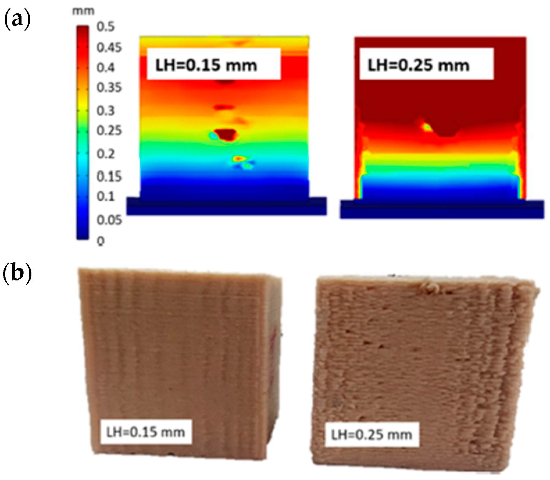
  74. Ding, S.; Zou, B.; Zhang, P.; Liu, Q.; Zhuang, Y.; Feng, Z.; Wang, F.; Wang, X. Layer thickness and path width setting in 3D printing of pre-impregnated continuous carbon, glass fibers and their hybrid composites. Addit. Manuf. 2024, 83, 104054. [Google Scholar] [CrossRef]
  75. Almeida, J.H.S.; Jayaprakash, S.; Kolari, K.; Kuva, J.; Kukko, K.; Partanen, J. The role of printing parameters on the short beam strength of 3D-printed continuous carbon fibre reinforced epoxy-PETG composites. Compos. Struct. 2024, 337, 118034. [Google Scholar] [CrossRef]
  76. Baechle-Clayton, M.; Loos, E.; Taheri, M.; Taheri, H. Failures and Flaws in Fused Deposition Modeling (FDM) Additively Manufactured Polymers and Composites. J. Compos. Sci. 2022, 6, 202. [Google Scholar] [CrossRef]
  77. Akhoundi, B.; Behravesh, A.H.; Bagheri Saed, A. An innovative design approach in three-dimensional printing of continuous fiber–reinforced thermoplastic composites via fused deposition modeling process: In-melt simultaneous impregnation. Proc. Inst. Mech. Eng. B J. Eng. Manuf. 2020, 234, 243–259. [Google Scholar] [CrossRef]
  78. Lupone, F.; Padovano, E.; Venezia, C.; Badini, C. Experimental Characterization and Modeling of 3D Printed Continuous Carbon Fibers Composites with Different Fiber Orientation Produced by FFF Process. Polymers 2022, 14, 426. [Google Scholar] [CrossRef]
  79. Croom, B.P.; Abbott, A.; Kemp, J.W.; Rueschhoff, L.; Smieska, L.; Woll, A.; Stoupin, S.; Koerner, H. Mechanics of nozzle clogging during direct ink writing of fiber-reinforced composites. Addit. Manuf. 2021, 37, 101701. [Google Scholar] [CrossRef]
  80. Muftu, S. Introduction. In Finite Element Method; Academic Press: Cambridge, MA, USA, 2022; pp. 1–8. [Google Scholar] [CrossRef]
  81. Zienkiewicz, O.C.; Taylor, R.L. The Finite Element Method Volume 1: The Basis; Wiley: Hoboken, NJ, USA, 2000; Volume 1. [Google Scholar]
  82. Li, S.; Sitnikova, E. Representative volume elements and unit cells. In Representative Volume Elements and Unit Cells: Concepts, Theory, Applications and Implementation; Woodhead Publishing: Sawston, UK, 2020; pp. 67–77. [Google Scholar] [CrossRef]
  83. Shafighfard, T.; Cender, T.A.; Demir, E. Additive manufacturing of compliance optimized variable stiffness composites through short fiber alignment along curvilinear paths. Addit. Manuf. 2021, 37, 101728. [Google Scholar] [CrossRef]
  84. Li, N.; Link, G.; Wang, T.; Ramopoulos, V.; Neumaier, D.; Hofele, J.; Walter, M.; Jelonnek, J. Path-designed 3D printing for topological optimized continuous carbon fibre reinforced composite structures. Compos. B Eng. 2020, 182, 107612. [Google Scholar] [CrossRef]
  85. Chen, Y.; Klingler, A.; Fu, K.; Ye, L. 3D printing and modelling of continuous carbon fibre reinforced composite grids with enhanced shear modulus. Eng. Struct. 2023, 286, 116165. [Google Scholar] [CrossRef]
  86. Chen, Y.; Ye, L. Topological design for 3D-printing of carbon fibre reinforced composite structural parts. Compos. Sci. Technol. 2021, 204, 108644. [Google Scholar] [CrossRef]
  87. Qian, S.; Liu, H.; Wang, Y.; Mei, D. Structural optimization of 3D printed SiC scaffold with gradient pore size distribution as catalyst support for methanol steam reforming. Fuel 2023, 341, 127612. [Google Scholar] [CrossRef]
  88. Date, A.W. (Ed.) Introduction. In Introduction to Computational Fluid Dynamics; Cambridge University Press: Cambridge, UK, 2005; pp. 1–16. [Google Scholar] [CrossRef]
  89. Hu, H.H. Chapter 10—Computational Fluid Dynamics. In Fluid Mechanics, 5th ed.; Kundu, P.K., Cohen, I.M., Dowling, D.R., Eds.; Academic Press: Boston, MA, USA, 2012; pp. 421–472. [Google Scholar] [CrossRef]
  90. Xu, X.; Ren, H.; Chen, S.; Luo, X.; Zhao, F.; Xiong, Y. Review on melt flow simulations for thermoplastics and their fiber reinforced composites in fused deposition modeling. J. Manuf. Process. 2023, 92, 272–286. [Google Scholar] [CrossRef]
  91. Wang, P.; Zou, B.; Xiao, H.; Ding, S.; Huang, C. Effects of printing parameters of fused deposition modeling on mechanical properties, surface quality, and microstructure of PEEK. J. Mater. Process Technol. 2019, 271, 62–74. [Google Scholar] [CrossRef]
  92. Shi, X.Z.; Huang, M.; Zhao, Z.F.; Shen, C.Y. Nonlinear fitting technology of 7-parameter Cross-WLF viscosity model. Adv. Mater. Res. 2011, 189–193, 2103–2106. [Google Scholar] [CrossRef]
  93. Yang, D.; Wu, K.; Wan, L.; Sheng, Y. A particle element approach for modelling the 3d printing process of fibre reinforced polymer composites. J. Manuf. Mater. Process. 2017, 1, 10. [Google Scholar] [CrossRef]
  94. Sun, X.; Sakai, M.; Yamada, Y. Three-dimensional simulation of a solid-liquid flow by the DEM-SPH method. J. Comput. Phys. 2013, 248, 147–176. [Google Scholar] [CrossRef]
  95. Monaghan, J.J. An Introduction to SPH. Comput. Phys. Commun. 1988, 48, 89–96. [Google Scholar] [CrossRef]
  96. Kanarska, Y.; Duoss, E.B.; Lewicki, J.P.; Rodriguez, J.N.; Wu, A. Fiber motion in highly confined flows of carbon fiber and non-Newtonian polymer. J. Nonnewton Fluid. Mech. 2019, 265, 41–52. [Google Scholar] [CrossRef]
  97. Zhang, L.; Zhang, H.; Wu, J.; An, X.; Yang, D. Fibre bridging and nozzle clogging in 3D printing of discontinuous carbon fibre-reinforced polymer composites: Coupled CFD-DEM modelling. Int. J. Adv. Manuf. Technol. 2021, 117, 3549–3562. [Google Scholar] [CrossRef]
  98. Wang, Z.; Smith, D.E. A fully coupled simulation of planar deposition flow and fiber orientation in polymer composites additive manufacturing. Materials 2021, 14, 2596. [Google Scholar] [CrossRef]
  99. Kermani, N.N.; Advani, S.G.; Férec, J. Orientation Predictions of Fibers Within 3D Printed Strand in Material Extrusion of Polymer Composites. Addit. Manuf. 2023, 77, 103781. [Google Scholar] [CrossRef]
  100. Advani, S.G.; Tucker, C.L. The Use of Tensors to Describe and Predict Fiber Orientation in Short Fiber Composites. J. Rheol. 1987, 31, 751–784. [Google Scholar] [CrossRef]
  101. Carreau, P.J.; De Kee, D.C.R.; Chhabra, R.P. Rheology of Polymeric Systems. In Rheology of Polymeric Systems; Carl Hanser Verlag GmbH & Co. KG: Munich, Germany, 2021. [Google Scholar] [CrossRef]
  102. Zhang, H.; Chen, J.; Yang, D. Fibre misalignment and breakage in 3D printing of continuous carbon fibre reinforced thermoplastic composites. Addit. Manuf. 2021, 38, 101775. [Google Scholar] [CrossRef]
  103. Zhang, K.; Zhang, H.; Wu, J.; Chen, J.; Yang, D. Improved fibre placement in filament-based 3D printing of continuous carbon fibre reinforced thermoplastic composites. Compos. Part A Appl. Sci. Manuf. 2023, 168, 107454. [Google Scholar] [CrossRef]
  104. Morvayová, A.; Contuzzi, N.; Casalino, G. Defects and residual stresses finite element prediction of FDM 3D printed wood/PLA biocomposite. Int. J. Adv. Manuf. Technol. 2023, 129, 2281–2293. [Google Scholar] [CrossRef]
  105. Ghnatios, C.; Fayazbakhsh, K. Warping estimation of continuous fiber-reinforced composites made by robotic 3D printing. Addit. Manuf. 2022, 55, 102796. [Google Scholar] [CrossRef]
  106. Struzziero, G.; Barbezat, M.; Skordos, A.A. Assessment of the benefits of 3D printing of advanced thermosetting composites using process simulation and numerical optimisation. Addit. Manuf. 2023, 63, 103417. [Google Scholar] [CrossRef]
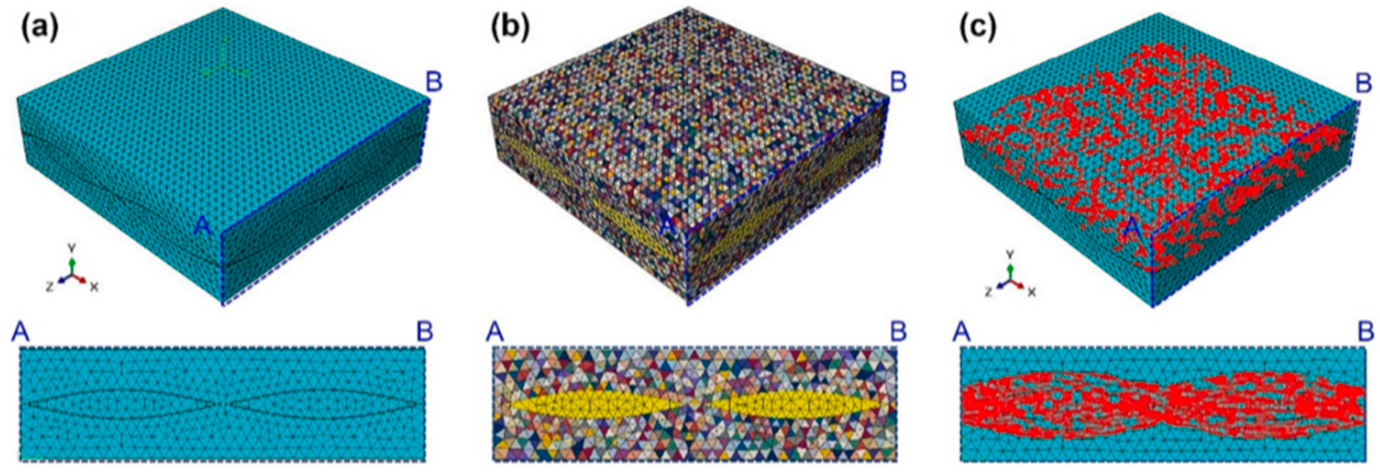
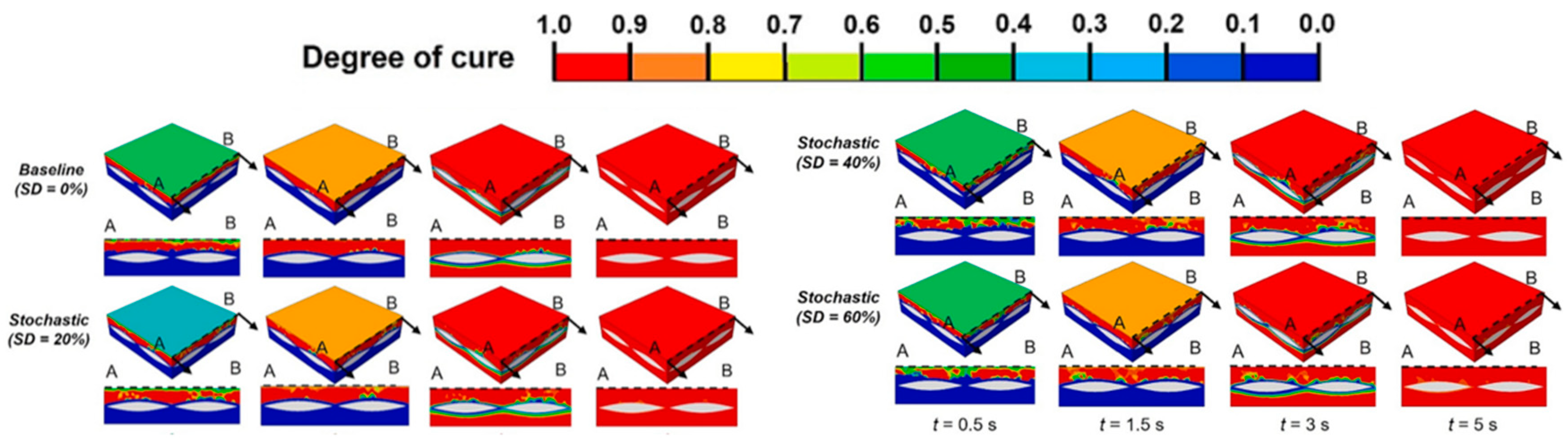
  107. Sharifi, A.M.; Kwon, D.J.; Shah, S.Z.H.; Lee, J. Modeling of frontal polymerization of carbon fiber and dicyclopentadiene woven composites with stochastic material uncertainty. Compos. Struct. 2023, 326, 117582. [Google Scholar] [CrossRef]
  108. Ross, S.M. Generating continuous random variables. In Simulation; Academic Press: Cambridge, MA, USA, 2023. [Google Scholar] [CrossRef]
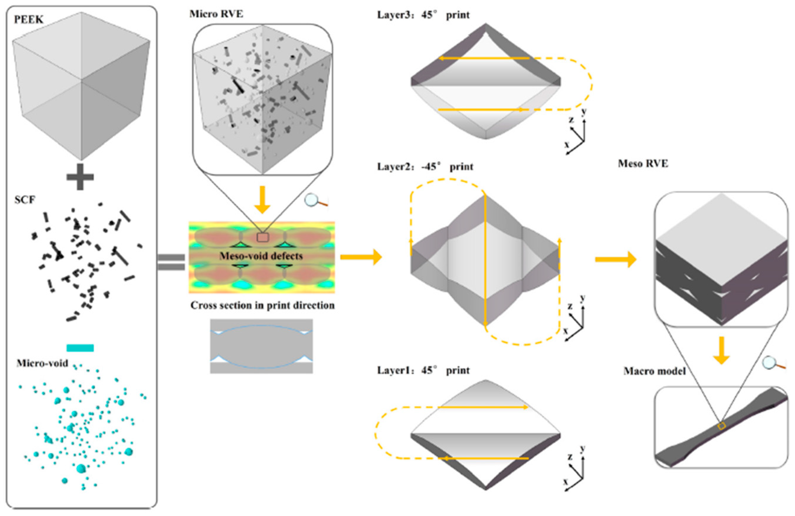
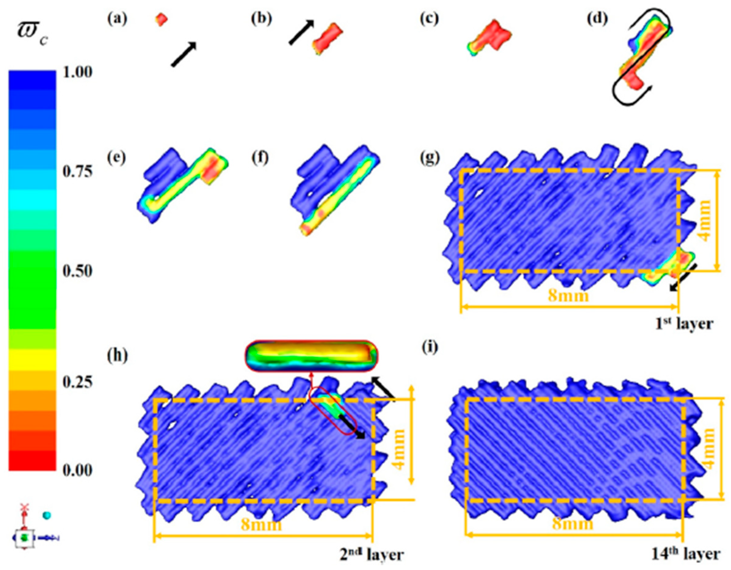
  109. Fu, Y.T.; Li, J.; Li, Y.Q.; Fu, S.Y.; Guo, F.L. Full-process multi-scale morphological and mechanical analyses of 3D printed short carbon fiber reinforced polyetheretherketone composites. Compos. Sci. Technol. 2023, 236, 109999. [Google Scholar] [CrossRef]
  110. Gao, C.Y. FE Realization of a Thermo-Visco-Plastic Constitutive Model using VUMAT in ABAQUS/Explicit Program. In Computational Mechanics; Springer: Berlin/Heidelberg, Germany, 2007. [Google Scholar] [CrossRef]
  111. Zhilyaev, I.; Grieder, S.; Küng, M.; Brauner, C.; Akermann, M.; Bosshard, J.; Inderkum, P.; Francisco, J.; Eichenhofer, M. Experimental and numerical analysis of the consolidation process for additive manufactured continuous carbon fiber-reinforced polyamide 12 composites. Front. Mater. 2022, 9, 1068261. [Google Scholar] [CrossRef]
  112. Nakamura, K.; Katayama, K.; Amano, T. Some aspects of nonisothermal crystallization of polymers. II. Consideration of the isokinetic condition. J. Appl. Polym. Sci. 1973, 17, 1031–1041. [Google Scholar] [CrossRef]
  113. Lorenz, N.; Gröger, B.; Müller-Pabel, M.; Gerritzen, J.; Müller, J.; Wang, A.; Fischer, K.; Gude, M.; Hopmann, C. Development and verification of a cure-dependent visco-thermo-elastic simulation model for predicting the process-induced surface waviness of continuous fiber reinforced thermosets. J. Compos. Mater. 2023, 57, 1105–1120. [Google Scholar] [CrossRef]
  114. Grieder, S.; Zhilyaev, I.; Küng, M.; Brauner, C.; Akermann, M.; Bosshard, J.; Inderkum, P.; Francisco, J.; Willemin, Y.; Eichenhofer, M. Consolidation of Additive Manufactured Continuous Carbon Fiber Reinforced Polyamide 12 Composites and the Development of Process-Related Numerical Simulation Methods. Polymers 2022, 14, 3429. [Google Scholar] [CrossRef]
Figure 1. Principle of FDM with pure thermoplastics (a); reinforced thermoplastics (b) [38]. Reproduced with permission: Elsevier.
Jcs 08 00146 g001
Figure 2. Principle of continuous fiber DIW with a thermoset matrix [58]. Reproduced with permission: Elsevier.
Jcs 08 00146 g002
Figure 3. Principle of the in-situ impregnation of CFF (a); Prepreg (b) [71]. Under CC−BY Licensing 4.0.
Jcs 08 00146 g003
Figure 4. Physics of FFF processes [36]. Reproduced with permission: Elsevier.
Jcs 08 00146 g004
Figure 5. Design optimization for SCF/PETG specimen (a); path generation (b) [83]. Reproduced with permission: Elsevier.
Jcs 08 00146 g005
Figure 6. Tensile test for 0° orientation (a); path optimization SCF/PETG specimens (b) [83]. Reproduced with permission: Elsevier.
Jcs 08 00146 g006
Figure 7. Continuous flow paths for PETG/SCF specimens: virtual (a); physical (b) [83]. Reproduced with permission: Elsevier.
Jcs 08 00146 g007
Figure 8. Trajectory optimization for CCF structures with 40% infill (a); 60% infill (b) [85]. Reproduced with permission: Elsevier.
Jcs 08 00146 g008
Figure 9. von Mises stress diagram of structures made with different volume fractions for PA specimens (a); CCF-PA specimens (b) [85]. Reproduced with permission: Elsevier.
Jcs 08 00146 g009
Figure 10. Definitions for optimization (a); paths of CCF/SCF in the optimized part (b) [86]. Reproduced with permission: Elsevier.
Jcs 08 00146 g010
Figure 11. Structural stiffness of PA, SCF-PA, and CCF-PA specimens (a); peak load (b) [86]. Reproduced with permission: Elsevier.
Jcs 08 00146 g011
Figure 12. Methanol reactor geometry (a); discretization (b) [87]. Reproduced with permission: Elsevier.
Jcs 08 00146 g012
Figure 13. Reactor simulation for flow velocity (a); hydrogen concentration (b) [87]. Reproduced with permission: Elsevier.
Jcs 08 00146 g013
Figure 14. Computational fluid dynamics in the AM of composites: multi-phase transformation (a); extrusion process (b); deposition process (c) [90]. Reproduced with permission: Elsevier.
Jcs 08 00146 g014
Figure 15. Temperature plots in the printing head for PEEK (a); temperature above melting in the nozzle area (343 °C) (b); temperature at phase change (c); viscosity at phase change (d) [91]. Reproduced with permission: Elsevier.
Jcs 08 00146 g015
Figure 16. Model definition of GF-ABS AM (a); short GF/ABS flow simulation (b) [93]. Under CC−BY Licensing 4.0.
Jcs 08 00146 g016
Figure 17. Model definition for the continuous fiber fabrication of Nylon-CF (a); flow map of the continuous fiber fabrication of Nylon-CF (b) [93]. Under CC−BY Licensing 4.0.
Jcs 08 00146 g017
Figure 18. Tensile stress in the continuous fiber before deposition (a); after deposition (b) [93]. Under CC−BY Licensing 4.0.
Jcs 08 00146 g018
Figure 19. Fiber flow into the nozzle at 0.25 s (a); 0.55 s (b); graphics of orientation (c) [96]. Reproduced with permission: Elsevier.
Jcs 08 00146 g019
Figure 20. Fiber orientation and flow in the cylindrical nozzle with different fiber diameters: 0.15 mm (a); 0.3 mm (b); 0.5 mm (c) [96]. Reproduced with permission: Elsevier.
Jcs 08 00146 g020
Figure 21. Definition of areas in the printing nozzle [97]. Under CC−BY Licensing 4.0.
Jcs 08 00146 g021
Figure 22. Probability density function (a); coordination number for SCF-PA for 0.12 mm raster width (b); 0.24 mm width (c); 0.35 mm width (d) [97]. Under CC−BY Licensing 4.0.
Jcs 08 00146 g022
Figure 23. Fiber flow for L = 0.24 mm and Vf = 26.68% (a); contact forces in the nozzle (b) [97]. Under CC−BY Licensing 4.0.
Jcs 08 00146 g023
Figure 24. A 2D schematic representation of matrix flow of composite filaments [98]. Under CC−BY Licensing 4.0.
Jcs 08 00146 g024
Figure 25. Fiber orientation of SCF on the X direction (A); view (B); and XZ view (C) [99]. Reproduced with permission: Elsevier.
Jcs 08 00146 g025
Figure 26. Geometric description (a); strand form (b) [99]. Reproduced with permission: Elsevier.
Jcs 08 00146 g026
Figure 27. Printing layer shape and fiber orientation (X-axis; (A,C,E)), Y-axis (B,D,F) [99]. Reproduced with permission: Elsevier.
Jcs 08 00146 g027
Figure 28. Straight and angular change direction in CCF: normal stress (a); shear stress (b); contact pressure (c); bottom view (d) [102]. Reproduced with permission: Elsevier.
Jcs 08 00146 g028
Figure 29. Angular variation effect on residual stress [102]. Reproduced with permission: Elsevier.
Jcs 08 00146 g029
Figure 30. Radius variation effects on residual stress [102]. Reproduced with permission: Elsevier.
Jcs 08 00146 g030
Figure 31. FEA setup process of CFF [103]. Under CC−BY Licensing 4.0.
Jcs 08 00146 g031
Figure 32. Transverse plastic strain: M-nozzle (a); R-nozzle (b) [103]. Under CC−BY Licensing 4.0.
Jcs 08 00146 g032
Figure 33. Transverse shear strain: M-nozzle (a); R-nozzle (b) [103]. Under CC−BY Licensing 4.0.
Jcs 08 00146 g033
Figure 34. Logarithmic strain: M-nozzle (a); R-nozzle (b) [103]. Under CC−BY Licensing 4.0.
Jcs 08 00146 g034
Figure 35. Normal plastic strain on the circular path (R = 10 mm): M-nozzle (a); and R-nozzle (b) [103]. Under CC−BY Licensing 4.0.
Jcs 08 00146 g035
Figure 36. Normal strain on circular path (R = 2.5 mm) on: M-nozzle (a); R-nozzle (b) [103]. Under CC−BY Licensing 4.0.
Jcs 08 00146 g036
Figure 37. Strains on non-planar deposition: M-shaped nozzle (a); R-shaped nozzle (b) [103]. Under CC−BY Licensing 4.0.
Jcs 08 00146 g037
Figure 38. Residual displacements of the PLA–wood composite: simulation (a); experimental (b) [104]. Under CC−BY Licensing 4.0.
Jcs 08 00146 g038
Figure 39. Residual stress on PLA–wood specimens [104]. Under CC−BY Licensing 4.0.
Jcs 08 00146 g039
Figure 40. Temperature 3.5 s after completing the specimen [104]. Under CC−BY Licensing 4.0.
Jcs 08 00146 g040
Figure 41. Temperature field for CCF-PEEK for different thicknesses: 0.14 mm/layer (a); 0.28 mm/layer (b) [105]. Reproduced with permission: Elsevier.
Jcs 08 00146 g041
Figure 42. Raster deflection for CCF-PEEK for 11th trajectory (a); 15th trajectory (b); 23rd trajectory (c); 25th trajectory (d) [105]. Reproduced with permission: Elsevier.
Jcs 08 00146 g042
Figure 43. Printing bed temperature effects on warping for CCF-PEEK: 145 °C (a); 150 °C (b); 155 °C (c); 160 °C (d) [105]. Reproduced with permission: Elsevier.
Jcs 08 00146 g043
Figure 44. Deposition temperature effect on warping CCF-PEEK for Tdeposition = 390 °C (a); Tdeposition = 400 °C (b); Tdeposition = 410 °C (c); Tdeposition = 420 °C (d) [105]. Reproduced with permission: Elsevier.
Jcs 08 00146 g044
Figure 45. Printing speed effect on warping CCF-PEEK for υ = 1 mm/s (a); υ = 3 mm/s (b); υ = 5 mm/s (c); υ = 7 mm/s (d) [105]. Reproduced with permission: Elsevier.
Jcs 08 00146 g045
Figure 46. Process simulation setup for thermoset composites (a); pseudo-code of the algorithm used for the ABAQUS link (b) [106]. Under CC−BY Licensing 4.0.
Jcs 08 00146 g046
Figure 47. Contour of temperature distribution for thermoset composites (a); curing status distribution for thermoset composites (b); USDFLD and HETVAL coupling subroutines coupling (c) [106]. Under CC−BY Licensing 4.0.
Jcs 08 00146 g047
Figure 48. Meso-scale RVE frontal polymerization thermoset composite element (a); script for stochastic material setup (b) [107]. Reproduced with permission: Elsevier.
Jcs 08 00146 g048
Figure 49. Material hypotheses in frontal polymerization with the following: deterministic properties (a); stochastic Properties (b); deterministic properties with 3% void (c) [107]. Reproduced with permission: Elsevier.
Jcs 08 00146 g049
Figure 50. Curing simulation of frontal polymerization composites: XY plane heat source (a) [107]. Reproduced with permission: Elsevier.
Jcs 08 00146 g050
Figure 51. Defects caused by the thermal splatter simulation and experiment for a layer height of 0.25 mm (a) and a layer height of 0.15 mm (b) [104]. Under CC−BY Licensing 4.0.
Jcs 08 00146 g051
Figure 52. Defect simulation for cubical PLA–wood specimens for layer height = 0.25 mm: pultrusion (a); sinkholes (b); failure of lower edges (c) [104]. Under CC−BY Licensing 4.0.
Jcs 08 00146 g052
Figure 53. Multi-scale analysis of SCF-PEEK [109]. Reproduced with permission: Elsevier.
Jcs 08 00146 g053
Figure 54. Solidification simulation for SCF-PEEK specimens: single element trajectory (a,b); single layer changing direction trajectory (cg); next layer deposition (h,i) [109]. Reproduced with permission: Elsevier.
Jcs 08 00146 g054
Figure 55. Porosity simulation on CCF-PA12 fixture: 90° area (a); base area (b); complete part (c) [111]. Under CC−BY Licensing 4.0.
Jcs 08 00146 g055
Figure 56. Surface profile numerical model for thermoset composites [113]. Under CC−BY Licensing 4.0.
Jcs 08 00146 g056
Figure 57. Simulation results for void pressure (a); porosity (b); fiber fraction (c); elastic modulus at the heat deflection temperature (2 MPa, 175 °C) (d) [114]. Under CC−BY Licensing 4.0.
Jcs 08 00146 g057
Table 1. Technological parameters for AM composites [73,74,75,76,77,78,79].
No.Technological ParametersDefects Induced in the StructureInfluenced Characteristic
1.Slicing StrategyVoids Creation/Fiber Interruptions/Fiber OrientationMechanical Strength
2.Extrusion TemperatureWarping/Residual Stresses/Nozzle CloggingPrecision, Mechanical Strength
3.Nozzle Diameter Fiber Volume Content/Fiber Orientation Mechanical Strength
4.Printing-Bed TemperatureDelamination/Residual StressesPrecision/Mechanical Strength/Surface Defects
5.Layer HeightWarping, Surface Defects, Voids, Delamination, Residual StressesPrecision, Mechanical Strength
6.Printing Speed Fiber Orientation/Void FormationMechanical Strength
Table 2. Categorization of the analyses for composite 3D printing.
No.Process PhaseSubjectFE ApproachApplication
1.Pre-ProcessingPath OptimizationTopological Optimization, Fiber Direction OptimizationTrajectory Definition/Optimization
2.AM ProcessExtrusionComputational Fluid DynamicsMelting Simulation
In-Nozzle Flow and Fiber Orientation
Nozzle Clogging Simulation
DepositionMulti-Physics (Thermo-Mechanical)First Layer Formation
SolidificationMulti-Physics (Thermo-Mechanical)Residual Stresses
Dimensional Accuracy
Curing Thermoset Composites
3.Post-ProcessingDefects and Post-processing TreatmentsMulti-Physics (Thermo-Mechanical)Internal Defects
Void Formation
Surface Roughness
Disclaimer/Publisher’s Note: The statements, opinions and data contained in all publications are solely those of the individual author(s) and contributor(s) and not of MDPI and/or the editor(s). MDPI and/or the editor(s) disclaim responsibility for any injury to people or property resulting from any ideas, methods, instructions or products referred to in the content.

