Abstract
The growing applicability of functionally graded materials is justified by their ability to contribute to the development of advanced solutions characterized by the material customization, through the selection of the best parameters that will confer the best mechanical behaviour for a given structure under specific operating conditions. The present work aims to attain the optimal design solutions for a set of illustrative 2D and 3D discrete structures built from functionally graded materials using the Red Fox Optimization Algorithm, where the design variables are material parameters. From the results achieved one concludes that the optimal selection and distribution of the different materials’ mixture and the different exponents associated with the volume fraction law significantly influence the optimal responses found. To note additionally the good performance of the coupling between this optimization technique and the finite element method used for the linear static and free vibration analyses.
1. Introduction
Functionally graded materials (FGMs) are usually particle composite materials, in which their constituent material volume fractions vary continuously according to given spatial coordinates [1,2]. This material concept emerged in Japan in 1984 for application as a thermal barrier material, capable of withstanding high-temperature gradients [2,3,4]. In a more general perspective, these composites’ properties and characteristics allow them to be used with increasing frequency in the transportation industry, namely in aircraft and spacecraft structures, as well as in the automotive and marine industries. Other applications include electronic and medical pieces of equipment and in a quite transversal manner their use as thermal coatings for engines and turbines, among others. FGM are in general made from different constituent materials, namely ceramic and metallic material phases which have shown to be appropriate to operate as a thermal barrier [5,6,7]. The composition of these materials often varies from one surface rich in material A to another surface rich in material B, with a certain distribution between the two surfaces, resulting in a continuous variation in the material microstructure. This continuous variation allows the effective properties of FGMs to have a gradual and smooth evolution, which makes it possible to minimize undesirable situations that occur in fibre-reinforced laminated structures due to their anisotropy, namely stress concentrations in the vicinity of material and geometric discontinuities and residual stresses, which can lead to delamination, cracks in the matrix and separation of adhesive bonds [8,9,10,11,12].
However, depending on the applications’ characteristics, other material mixtures have been utilized as illustrated in the studies developed by [13,14,15,16,17], where mixtures of different metallic, polymeric, and ceramic materials were used. The FGM concept extended to materials with specific biocompatible characterisics can also be found with an increasing frequency, namely in [18,19,20], among others.
Considering the wide range of potentially variable parameters involved in a generic structure design, obtaining better solutions according to certain objectives for a given structure subjected to specific loads and boundary conditions may be a complex task. The increasing complexity and non-linearity of real problems require the development of efficient optimization methods with high accuracy and response speed combined with low computational cost [21,22]. Metaheuristics are optimization techniques that are often based on natural phenomena [22] and have shown to be adequate to address such complex problems. They are generally based on rules translated from the observation of what occurs in nature considering randomness, to mimic some of the characteristics of biological behaviour, and natural or physical phenomena [23].
When one talks about FGM optimization [24], the parameters normally considered as design variables characterize, on one hand, the evolution of the volume fractions of the material (the power law exponent or other laws) and, on the other hand, the geometric characteristics of the cross-section. The objective functions usually aim at maximizing or minimizing mass, maximum stresses, resistance to fracture, behaviour in situations with temperature gradients, and dynamic response in free and forced vibration, or buckling loads [2,25]. To illustrate this, one can refer to the work conducted in [5] where a model was developed for the longitudinal variation of the composition of a metal/ceramic FGM, to optimize the heat flow through this material as a function of the material composition profile. Another work carried out in [2], the influence of the dimension for which the volume fraction is defined, in a thin cantilever beam with a hollow profile was studied, being found that the maximization of the natural frequencies, was benefited by a material mixture distribution in the longitudinal direction rather than considering it in the thickness direction, which has been more commonly studied. A very recent work on topology optimization of micro and macroscale topology optimization of FGM lattice structures was presented by [26]. Other studies focusing on optimizing the mechanical behaviour of composite structures have been studied by several researchers [27,28] considering a wide variety of optimization techniques.
The optimization algorithm considered in the present work consists of a very recent technique which has been used so far, mainly in the context of medical science applications, for example for lung x-ray image segmentation [29], electroencephalogram signals classification [30], in computer science for example, to optimize hyperparameters of deep-learning models [31], and very scarcely in engineering for example for the optimization of phase equilibrium and stability of chemical systems [32] or to estimate optimal model parameters of solid oxide fuel cells [33].
However, no published work was found considering the use of this technique in the optimization of the mechanical behaviour of structures in general, nor to optimize the innovative height functionally graded structures considered in the present work, in particular.
This work is a natural sequence of the study conducted in [34], which studied the influence of the power law exponent and the effective properties estimation, on the static and dynamic behaviour of two-dimensional planar structures in the free vibration regime. By generalizing and combining the previously developed structural analysis application with the present metaheuristic optimization technique, it becomes possible to optimizing the desired structure behaviour without extensive parametric studies and with less probability of achieving the effective best configuration.
The selection of the present optimization metaheuristic is mainly related to the conclusion drawn in [35] which stated that this technique shows better exploration and exploitation characteristics when compared with other techniques also analysed, namely the Genetic Algorithm, the Particle Swarm Optimization, the Grey Wolf Optimization, the Chimp Optimization Algorithm, the Butterfly Optimization Algorithm, the Whale Optimization Algorithm, the Fitness Dependent Optimizer and the Dragonfly Optimization Algorithm.
Hence, with this work, one aims to obtain the best performance in terms of maximum linear static displacements and fundamental frequencies for a set of two and three-dimensional structures in which the material gradient is a function of the vertical coordinate of the structure. From the authors’ knowledge, no published work focused on optimizing these types of FGM structures, or even on using the Red Fox algorithm for structural optimization, was found.
The remainder part of this work is organized as follows: Section 2 describes the concept of the FGMs that will be used in the present study, Section 3 presents the displacement field, constitutive relations and equilibrium equations associated with the linear static and free vibrations analyses to be developed for each individual considered in the context of the populations-based optimization technique that will be presented in Section 4. The methodology is presented in Section 5 and Section 6 contains the case studies considered. Finally, in Section 7 some conclusions are drawn based on the results achieved.
2. Functionally Graded Materials
This study considers the optimization of FGM structures in which the material gradient is a function of the vertical coordinate of the structure (Y) [34]. The objective functions considered are minimizing the linear static displacements of selected points within the structures or maximizing their fundamental frequencies. Although it is possible to consider other design variables, for example, those of a geometrical nature, this work is focused on obtaining the material parameters’ configurations that will make it possible to achieve better structural responses without changing the structure’s geometry.
Figure 1 illustrates a two-dimensional frame-type structure where the material gradient through the Y direction, associated with the structure height, is represented.
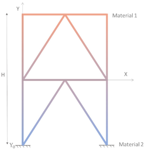
Figure 1.
Schematic Representation of a Structure Built in FGM with a Variation in Properties as a Function of the Structure’s Height.
If is the ordinate of the lower end of the structure, H corresponds to the maximum height of the structure, Y is the vertical coordinate that varies between 0 and H, and ey is the exponent of the power law that adjusts how the property variation along the vertical coordinate occur, the generic expression of the volume fraction can be written as:
When the operating conditions of a given structure are known, it is possible to combine not only the most appropriate geometric characteristics, but also, as this work aims to demonstrate, the best constituent materials from within a given set, and the best parameters that control the distribution of the mixture of constituent materials mixture throughout the structure, to optimizing specific structural requirements [8,9].
The effective properties of FGMs are estimated according to the Voigt Rule of Mixtures [8], which makes it possible to determine the average value of a generic material property as a weighted average of the corresponding constituent materials’ properties (), where the weights are their volume fractions, as in the expression [36]:
The sum of the volume fractions must be unitary in the case of dual-phase FGMs, considering the assumption that the material has no porosities. The expression that describes a material volume fraction () evolution will reflect how that material will be distributed in a specific direction or multiple directions, which for the present work is given by Equation (1).
3. Displacement Field, Constitutive Relations, and Equilibrium Equations
Considering the structures that will be studied, one has to consider the first-order shear deformation to model their kinematical modelling [17,18,19,20,21]. The displacement field corresponding to this theory can be written as follows:
The terms, correspond, respectively, to the longitudinal (direction ) and transverse (directions and ) displacements of the beam’s centreline in the and planes, corresponds to the torsion angle, and and correspond to the rotation of the beam’s centre plane in a direction perpendicular to the plane and planes, respectively. Considering the Elasticity Theory for small deformations, the corresponding deformation field is written as:
The remaining strains , and are null, and the corresponding constitutive relations for a generic FGM are described as [36,37]:
where , and . represents the FGM Young’s modulus and the FGM Poisson’s ratio. The shear correction factor is set to .
Considering the aim of the present work, one has to use the principle of Hamilton to derive the equilibrium equations, which can be written as:
with standing for the kinetic energy, for the elastic strain energy and for the work done by the forces applied to the system. These quantities can be written as:
where represents the FGM density, stands for the punctual generalized forces and the generalized degrees of freedom. From the minimization of the Lagrangean functional, one achieves the equilibrium equations at the element level:
which, for linear static analysis or for free vibration analysis will be written as:
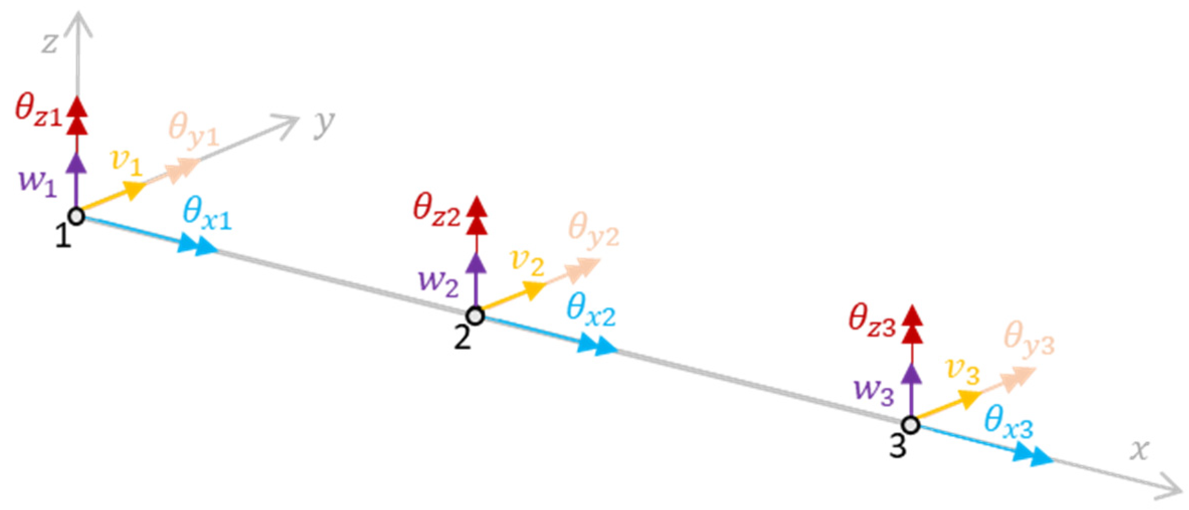
These equilibrium equations were implemented using quadratic beam elements with six degrees of freedom per node—the axial () and the transverse () displacements and the rotations (), all to the midplane surface of the beam element. Figure 2 schematically shows the beam element in the three-dimensional space and the degrees of freedom associated with each node [38,39,40,41,42].

Figure 2.
Quadratic Beam Element and its Degrees of Freedom.
Further details on the implementation of the beam-bar element used to model these structures can be found in [34].
4. Structural Optimization
A generic optimization problem can be stated as:
where is the objective function and is the vector of the design variables. Besides the side constraints associated with the design variables, the inequality and equality behavioral constraints are, respectively, designated as and .
In the present paper, the optimizations that are intended to be carried out are related to the minimization of the static displacements of specific points for a set of structures or the maximization of their fundamental frequencies. To this purpose one considers a metaheuristic optimization technique, the red fox optimization (RFO) algorithm.
Red Fox Metaheuristic Algorithm
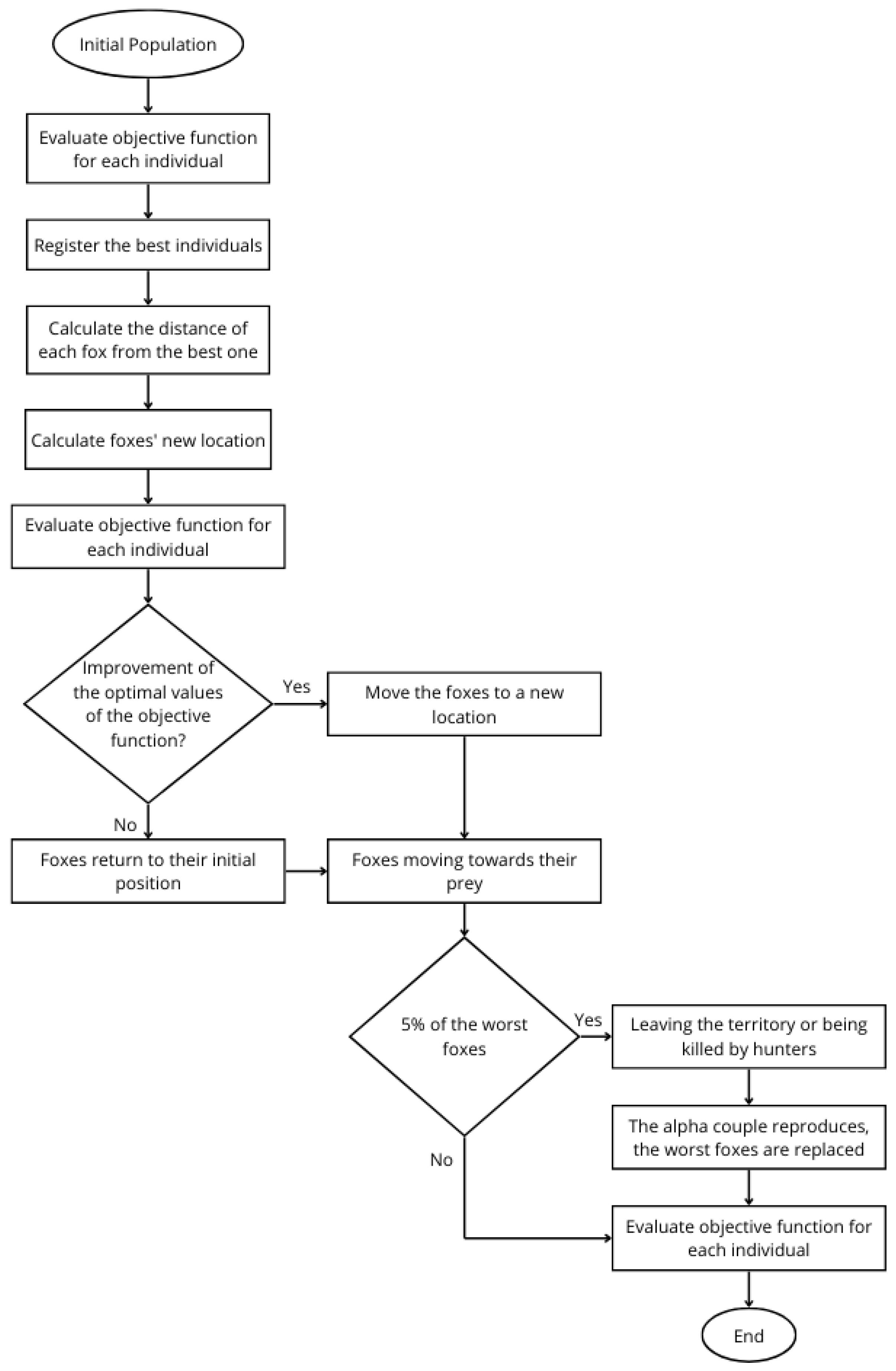
The red fox is a predator that hunts not only wild animals, but also farm animals, and in turn can be hunted by humans who intercept them in these attacks. The relationships between prey and predators and even between individuals in the same pack can be mimicked mathematically with a view to optimization, since only the fittest individuals survive to hunt in the different territories and to form a new pack elsewhere. The proposed model by [22] assumes that the optimization domain is comparable to hunting regions. Foxes have a hunting mechanism that can be considered in a first global search and then a local search. In addition to these two phases, a population control model has also been proposed, simulating the group leaving for another location or being killed by hunters. For this, the two best individuals are selected to reproduce and replace the weakest elements in each iteration. This mechanism allows the model to cover the entire domain to reach the global extreme, thus minimizing the risk of being confined to local extremes [22]. The algorithm is structured in a logical set of five steps as follows:
Step 1—Initial Population: The population is created with a selected number of foxes, which will be constant in each iteration. Each element is represented by , where i corresponds to the identification of the individual in the population, j represents the coordinate according to the dimension of the results space, and t is the current iteration. Based on the evaluation of the population generated through the objective function, the best individuals that provide the best solution are recorded, originating the population of the first iteration.
Step 2—Global Search: The members of the pack move to remote locations searching for food, and the information they collect is later shared with the other members to ensure their survival and development. The exploration of the surrounding territory is modelled on the basis of the objective function, and it is assumed that the best element explores the most interesting territories and shares this information with the group. Thus, the best individual in the population is recorded and the Euclidean distance of each of the other foxes is calculated using:
Individuals will move towards the fittest red fox through:
where α is a randomly generated parameter for all the individuals in each iteration, belonging to the interval [0, ]. At this point, the new population is evaluated using the objective function, and if the optimal values are better, the individuals take new positions, otherwise they return to the starting position. This simulates the path that the remaining members of the group will have to follow, after the information has been shared by the elements that have explored the surrounding territories, in which they must continue searching in promising areas, corresponding to step 3. The model also predicts the death of the worst individuals in the population, or the reproduction of the best individuals according to the equations in step 4.
Step 3—Local Search: When foxes spot prey, they try to approach it slowly in a circular motion so as not to be seen, until they are close enough to catch it. This behaviour is modelled using the parameter μ. This parameter is randomly generated in the interval [0, 1] and simulates the possibility of the fox being seen by the prey during the approach movement. For , the fox approaches the prey, otherwise it moves away. The movement of observation and approach of each individual to the prey was approximated using a modified Cochleoid equation, through the parameters and , where is randomly generated for each iteration in the interval [0, 0.2], and characterizes the change in distance to the prey, and models the angle of vision of each individual and is randomly generated in the interval [0, 2π] for all individuals. The radius of vision () of the foxes is obtained by:
where is a random value between [0, 1] generated at the start of the algorithm and characterises the influence of atmospheric conditions. For the individuals in the population, their movement is modelled using the system of Equation (14) for spatial coordinates, where each angular value is randomly generated in the interval [0, 2π].
Step 4—Reproduction and Pack Abandonment: For the dynamic control of the population, five per cent of the worst individuals in the population are selected according to the objective function, to introduce small changes to the pack. As these are the worst individuals, it is assumed that they have either moved territory or been killed by hunters; however, to ensure that the population is constant, the worst individuals are replaced by new individuals. In each iteration, the two best individuals (the alpha couple) are selected, and , and the centre of their habitat and diameter are calculated:
For each iteration, a random parameter is generated within the interval [0, 1], which defines the replacements of individuals. For , new individuals are introduced into the population, otherwise the alpha couple reproduces. In the first case, it is assumed that new family members will move to other regions, being able to reproduce. In the second case, new individuals are the result of the reproduction of the alpha couple, which results in:
Step 5—Evaluating each individual according to the objective function—From the objective function, the optimal values are recorded. For further details on the algorithm, please consult the corresponding literature [22].
5. Methodology
The generic goal of the optimization process is to determine the design parameter configuration that provide the best structure response, concerning a specific objective function to study.
In the present work, the studies developed have been structured into two types: the first considering only one design variable and the other considering four design variables. Both are, related to the material constitution of the FGM structures. In the first stage, the optimization process is related to determining the exponent of the power law that corresponds to the best behaviour of the structure for a given pair of materials. This design variable was assumed to vary in a continuous manner in the interval [0.1, 10].
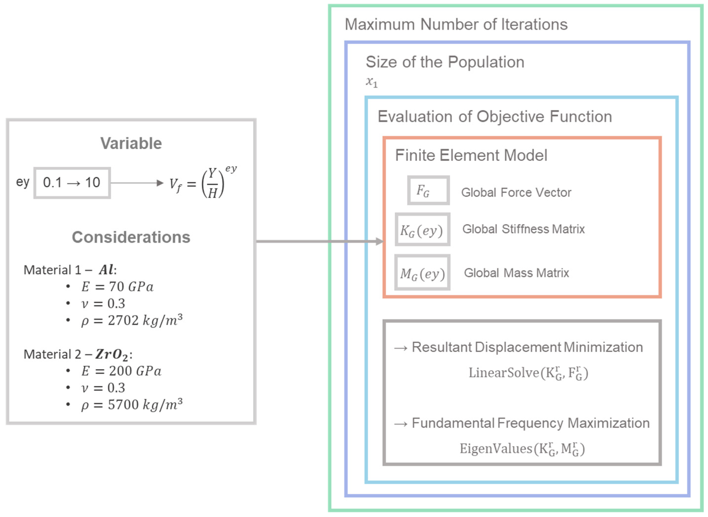
The procedure is schematically represented in Figure 3 and highlights the construction of the finite element model for the specific data associated with each of the individuals of the population, within each optimization iteration.
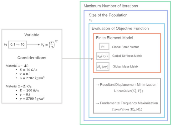
Figure 3.
Schematic diagram representation of the interaction between the finite element calculation and the optimization algorithm in the one-design variable model.
As observed in this case, the FGM structure is made of aluminum and zirconia, and the design variable, the power law exponent, varies within the mentioned interval. The rule of mixtures considers that the power law’s volume fraction is directly associated with the distribution of metallic material along the height of the structure.
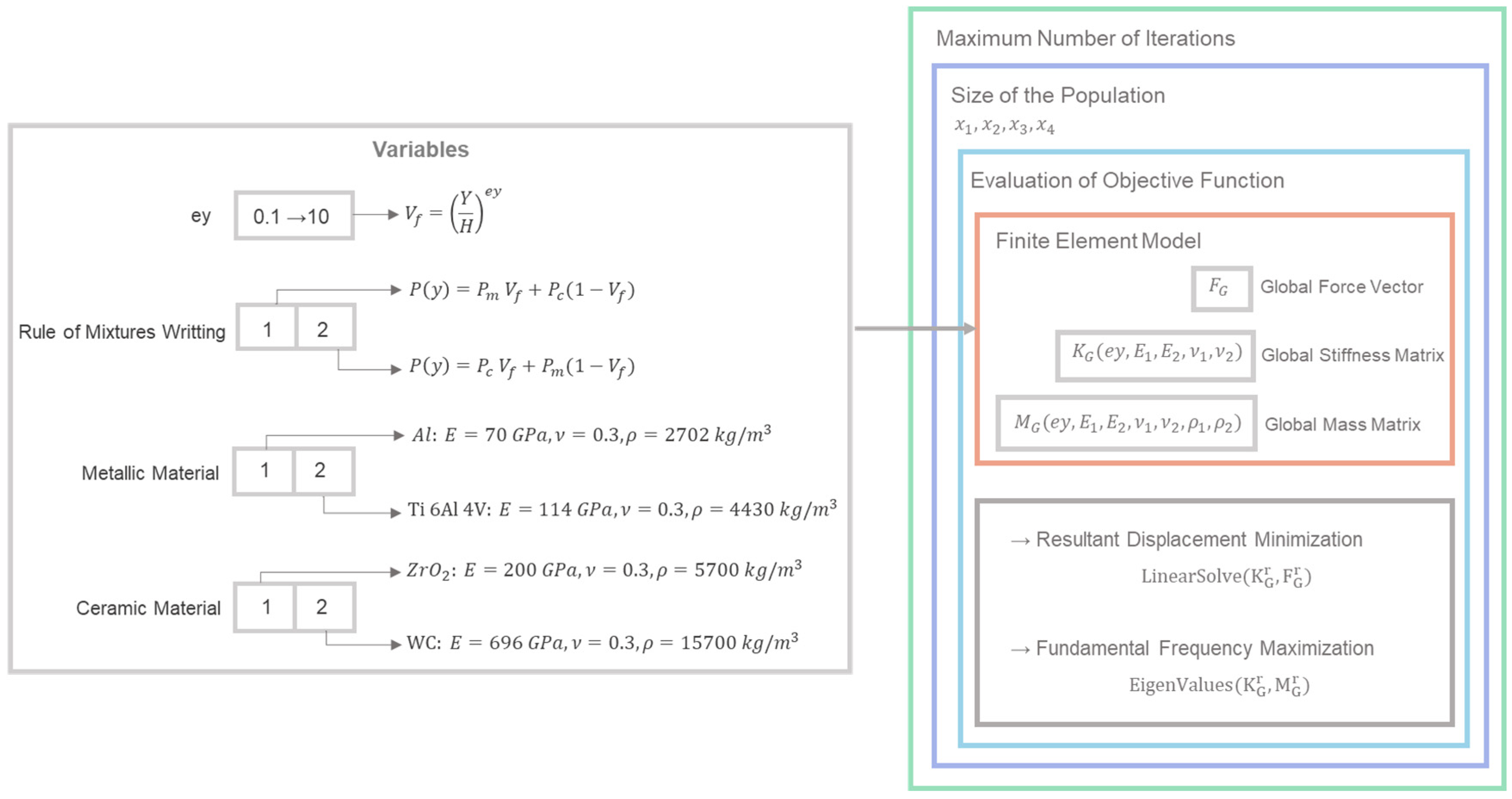
In the second stage, one considers a wider range of possibilities concerning the nature and number of design variables. Hence, in this case, it is possible to have different pairs of constituent materials to the resulting FGM, and to write the rule of mixtures associating the volume fraction directly to one or another of those constituent materials. A schematic diagram representation for the four design variable model is presented in Figure 4.

Figure 4.
Schematic diagram representation of the interaction between the finite element calculation and the optimization algorithm in the four-design variable model.
So, in addition to the power law exponent, another three variables were added, which can only take integer values of 1 or 2. The first one corresponds to the writing of the rule of mixtures, i.e., if the random number assumes 1, the volume fraction characterizes the distribution of metallic material; if it assumes 2, then the volume fraction describes the ceramic material distribution. The second additional design variable defines the metallic material to be used, in this case, aluminium and titanium, also randomly selected. The last additional design variable defines the possible ceramic material to use; zirconia and tungsten carbide were considered as options in the present study. For these three additional design variables introduced, that can only take the values {1, 2}, the expression that characterizes the update of the individual position in each iteration of each algorithm is adjusted by rounding it to the nearest integer value.
The optimization procedure is illustrated in a summarized manner, via the flowchart depicted in Figure 5.
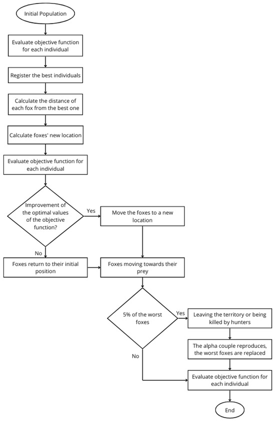
Figure 5.
Flowchart of the Red Fox Algorithm.
The present work thus considers the coupling between the red fox’s optimization technique and the finite element method that enables carrying out the necessary linear static and free vibration analyses for each individual, within each population.
In this work, which constitutes a first study in this context, a single-objective approach is considered. Also, besides the side constraints associated with each of the design variables space, possible behavioural constraints are not considered.
6. Results and Discussion
This section presents two verification cases, considering benchmark functions to illustrate the performance of the optimization technique. These cases are then followed by two additional performance assessment studies on FGM structures, where the results achieved via optimization processes, are compared with the trends obtained via parametric studies.
After, one conducts a set of case studies, to minimize specific points’ displacements in a certain structure or maximise their fundamental frequencies. The material properties used in the optimization cases next presented are the ones in Figure 3 and Figure 4.
6.1. Verification Cases
To verify the red fox optimization technique implemented, two studies are first presented using multimodal benchmark functions usually considered for this kind of verification purposes: the “Sum of Squares” function and the “Rastringin” function.
- Case 1—“Sum of Squares” Benchmark function
The optimal values obtained through the implementation of this algorithm in the present work were checked against those obtained by [22], where each function was evaluated in 100 independent runs, 100 iterations and for 100 individuals.
The first 20 independent runs out of 100 (presented in Appendix A) were carried out for the “Sum of Squares” function, using 20 design variables, considering 100 iterations and 100 individuals. The results obtained and their characteristics are shown in Table 1.

Table 1.
Characteristics of the Benchmark Function “Sum of Squares”.
The results obtained are shown in Table 2.
Table 2.
Results of the Verification Study of the Sum of Squares Function with Dimension 20, using 20 Runs, 100 Iterations and Populations of 100 Individuals.
According to the results here presented and, in the Appendix A, one concludes that the behaviour of the optimization algorithm is very satisfactory, with average values for the global minima of the function in the different runs, close to the found in the literature and very close to the exact solution. The standard deviation shows a similar magnitude.
- Case 2—“Rastringin ”Benchmark function
For the second verification case study, related to the “Rastringin” function, 10 independent runs were carried out, using two design variables, considering 100 iterations and 100 individuals. The characteristics of this function and the analysed domain are shown in Table 3.
Table 3.
Characteristics of the Benchmark Function “Rastrigin”.
As can be concluded from the results shown in Table 4, the implemented optimization technique presents a very good performance, with an average value very close to the exact solution. Again, the standard deviation shows a similar magnitude.
Table 4.
Results of the Verification Study of the Rastrigin Function with Dimension 2, using 10 Runs, 100 Iterations and Populations of 100 Individuals.
6.2. Performance Assessment Studies
In the previous sub-section, one considered two different benchmark functions, and compared the results obtained with the ones by other authors. In the present sub-section one intends to complement the previous one, applying now the optimization technique to two FGM structures. To be able to conclude on the performance of the technique for this type of problem, one has first conducted parametric studies for each structure to show the influence of the exponent ey, followed by optimization processes where that exponent is the design variable. The objective of this procedure is to demonstrate that the optimization results respect the known trends shown in the parametric studies.
In both cases, the transverse cross-section of the elements is square, with a 20 mm edge dimension, and an aspect ratio of 30. Considering the good performance of the optimization technique, in previous verification studies, a series of 10 runs was conducted for each optimization process, using as optimization parameters, a population of 5 individuals and 10 iterations.
- Case 3—2D Truss—Analysis and Optimization
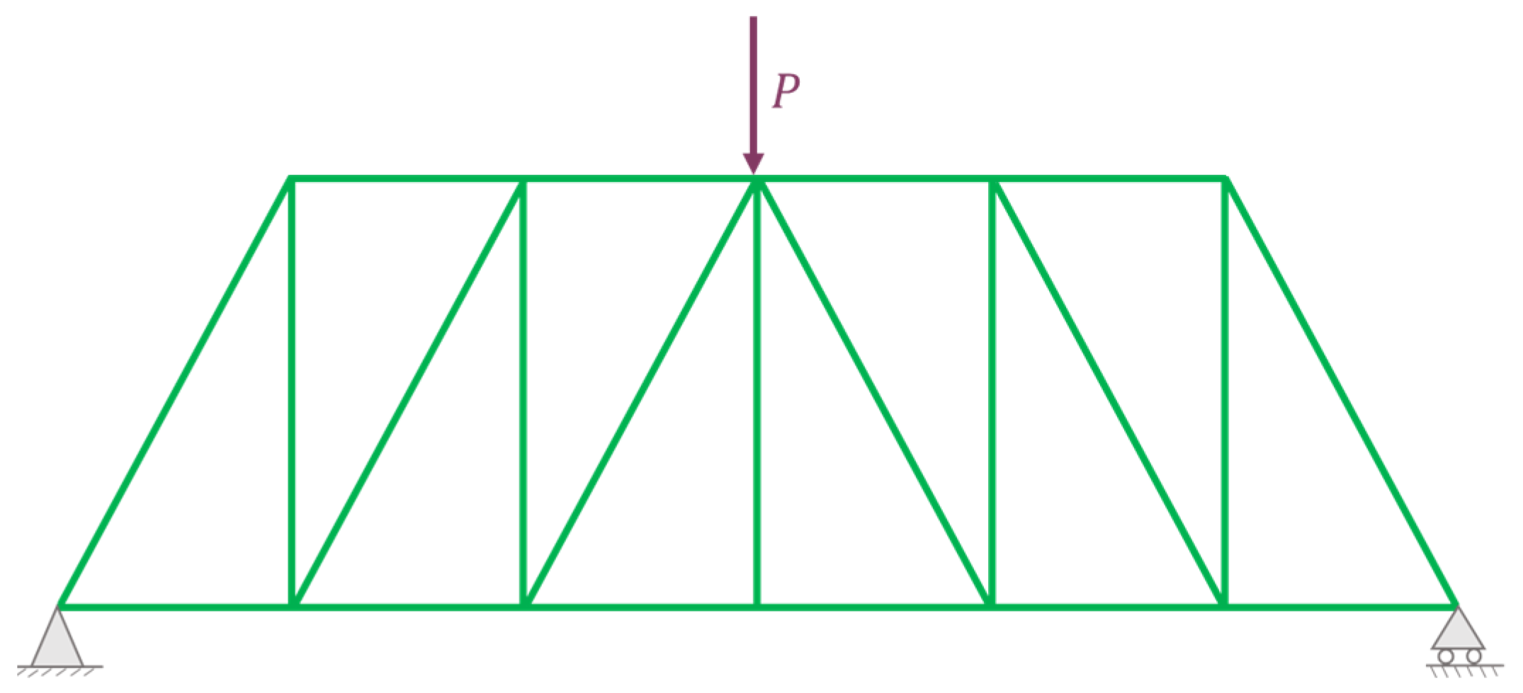
The first structure studied is a truss with 21 elements, subjected to a load P = 1 kN, as shown in Figure 6.
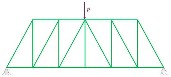
Figure 6.
Schematic Representation of 2D Truss.
Figure 7 presents the minimum discretization of the analysed 2D truss, with quadratic beam elements.
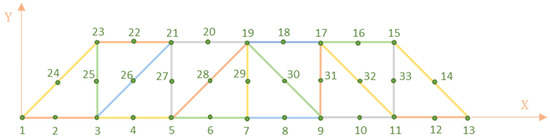
Figure 7.
Minimum Discretization of Two-dimensional Truss.
For this truss, the parametric studies conducted allow to conclude that the node where the largest resultant displacement occurs is at node 19, which corresponds to the node where the load is applied. Table 5 shows the resultant displacements of the mentioned node, and the fundamental frequency of the structure, for a set of exponents of the volume fraction power law.
Table 5.
Resultant Displacement of Node 19 in 2D Truss and Fundamental Frequency of the Truss.
Now, considering the optimization metaheuristic to maximize the fundamental frequency and to minimize the maximum resultant displacement, taking into account the exponent of the volume fraction expression as a design variable, the results presented in Table 6 are obtained.
Table 6.
Results of the Optimization Study for 2D Truss using RFO with one design variable.
To note that in the second and the fourth column one has the exponents of the volume fraction law obtained for the two optimization processes. The first process corresponding to the minimization of the maximum displacement (fmin), and the second process related to the fundamental frequency maximization (fmax).
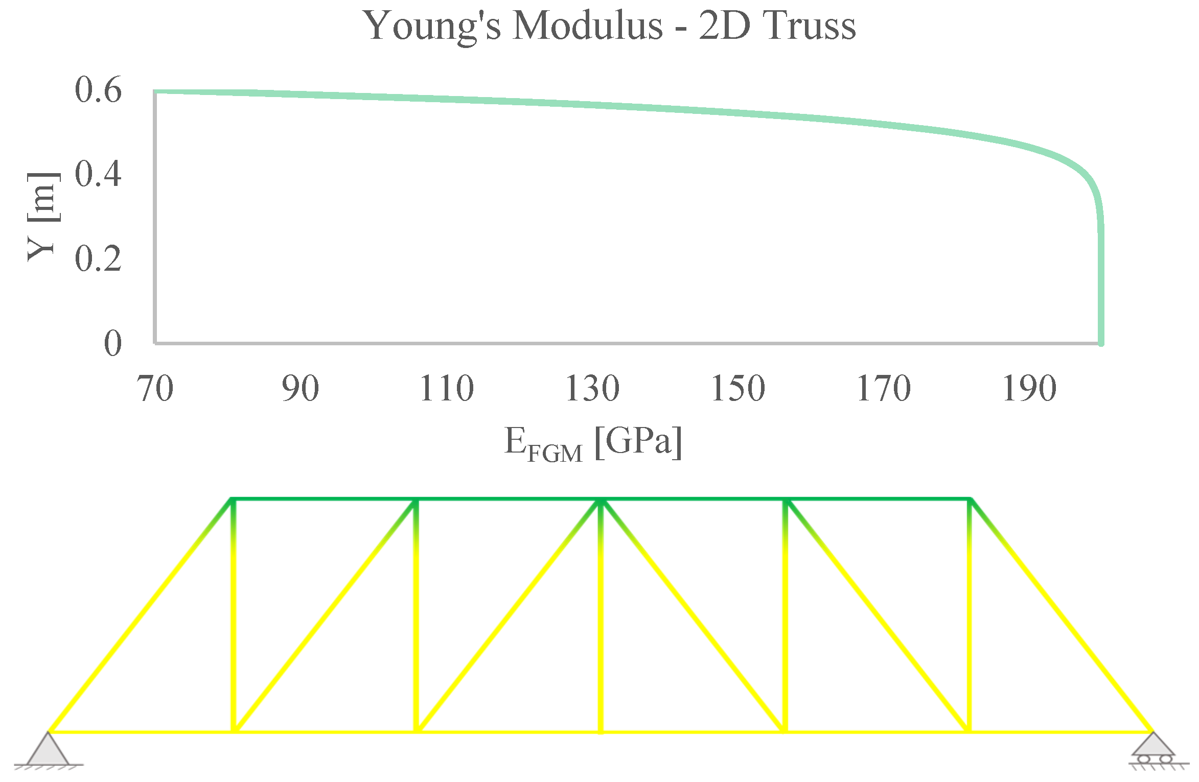
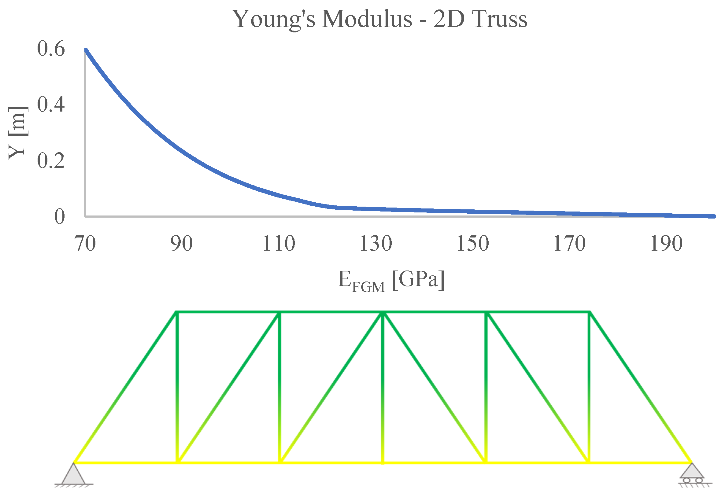
Figure 8 and Figure 9 show the evolution of Young’s modulus for the best solution found for minimizing the maximum resultant displacement and maximizing the fundamental frequency of the 2D truss, respectively, including a schematic representation of the structure’s configuration in relation to the constituent materials of the FGM.
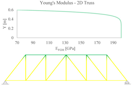
Figure 8.
Evolution of the Young’s Modulus of the 2D Truss for the Optimal Solution Found for Minimizing the Maximum Resulting Displacement using One Design Variable.

Figure 9.
Evolution of the Young’s Modulus of the 2D Truss for the Optimal Solution Found for Maximizing the Fundamental Frequency using the One Design Variable.
Regarding the results obtained, it should be noted that in a situation where the maximum resulting displacement is to be minimized, the optimum solution in terms of the power law exponent is the value 10, corresponding to the truss composed mostly of zirconia in the lower zone up to a height of approximately 0.4 m. On the other hand, if the fundamental frequency of the structure is to be maximized, the best dynamic behavior in the free vibration regime is achieved with an exponent of approximately 0.19.
The optimal design configurations for this structure are consistent with the results obtained in the parametric studies.
- Case 4—2D Frame—Analysis and Optimization
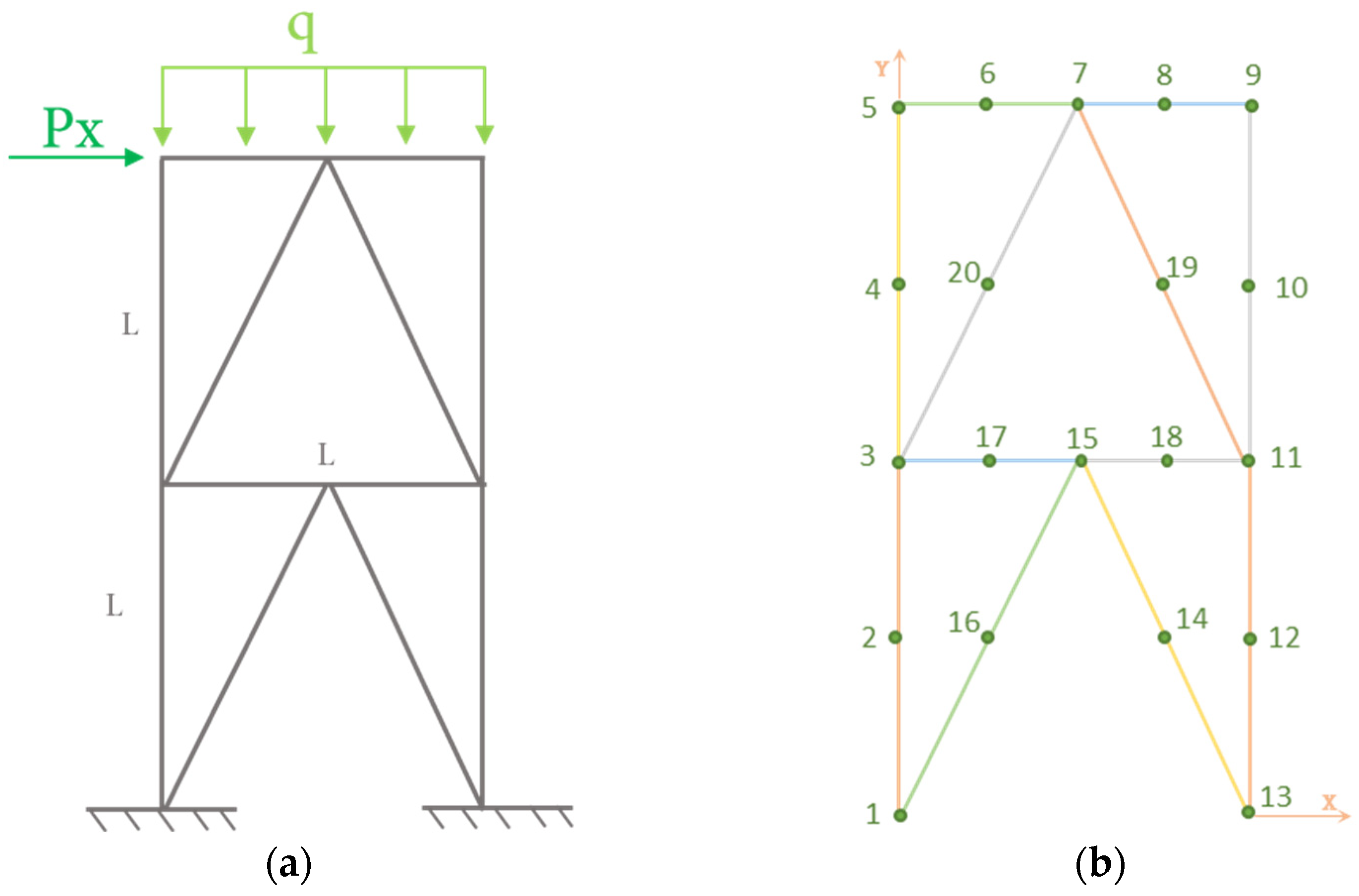
The second structure studied is a 2D frame constituted by 12 beams, the discretization of which, as well as other aspects such as geometrical configuration, boundary conditions and applied loading (Px = 50 N and q = 1000 N/m), are shown in Figure 10a,b.
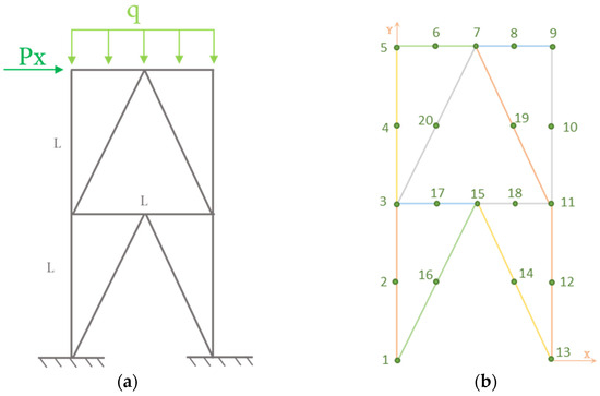
Figure 10.
(a) Schematic Representation of 2D Frame; (b) Minimum 2D Frame Discretization.
Table 7 shows the resultant displacement of node 10, as this is the node where the greatest resultant displacement occurs, and the first natural frequency of the structure.
Table 7.
Resultant displacement of Node 10 of Frame 2 and The fundamental frequency of the structure.
These results are again obtained by carrying out a parametric study for a set of pre-established exponent values. Now performing the optimization for each single-objective function, one obtains the results presented in Table 8.
Table 8.
Results of the optimization study for Frame 2 using RFO with one design variable.
Note that also in this table the second column contains the exponents of the volume fraction law obtained in the minimization of the maximum displacement, and the fourth column presents the exponents obtained in the fundamental frequency maximization.
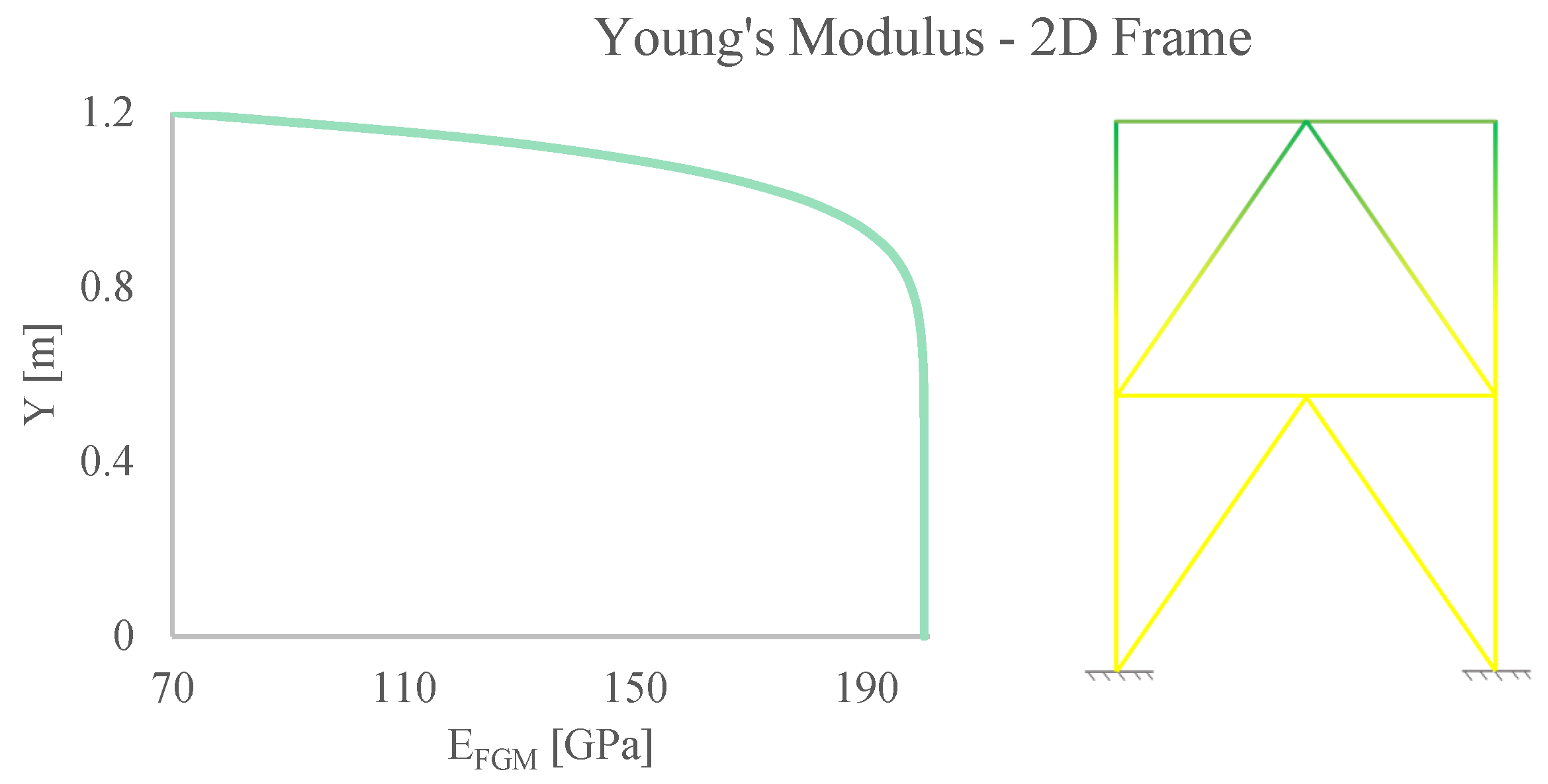
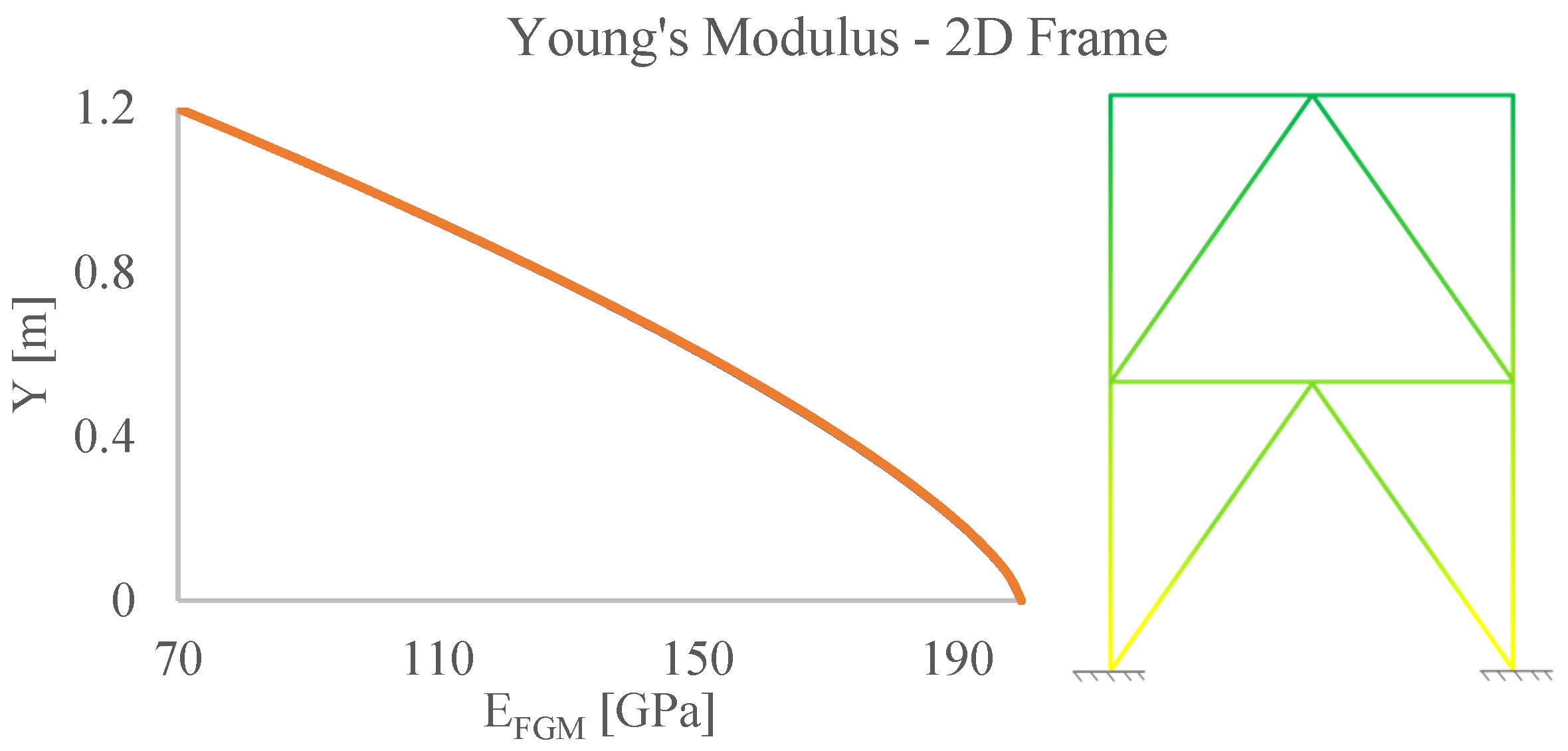
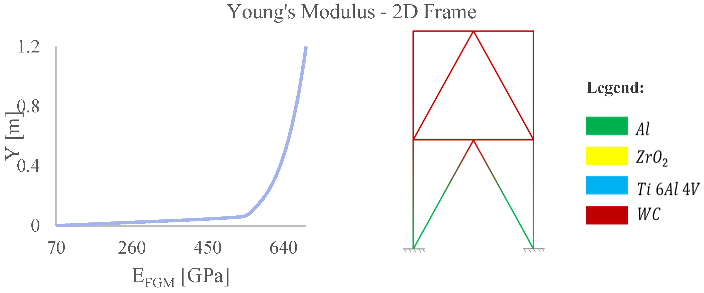
Figure 11 and Figure 12 show the evolution of the modulus of elasticity for the best solutions found to minimize the maximum resultant displacement and to maximize the fundamental frequency of the frame structure, respectively, including a schematic representation of the structure’s configuration concerning the constituent materials of the FGM.
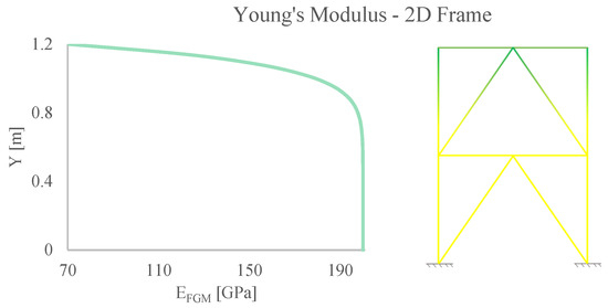
Figure 11.
Evolution of the Modulus of Elasticity of the 2D Frame by the Best Solution Found for Minimizing the Maximum Resulting Displacement using One Design Variable.
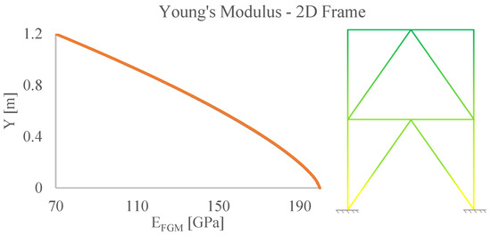
Figure 12.
Evolution of the Modulus of Elasticity of the 2D Frame by the Best Solution Found for Maximizing the Fundamental Frequency with One Design Variable.
Similarly to the cases previously studied, the optimum solution that characterizes a maximum resulting displacement in frame 2 is a power law exponent of 10. From the perspective of maximizing the fundamental frequency of the structure, it should be noted that the best configuration is the one that corresponds to an approximately linear distribution between the two materials that make up the FGM. Also, for this frame structure, the optimal design configurations are consistent with the results obtained in the parametric studies.
6.3. Optimization Case Studies—One Design Variable
The current sub-section presents the results of the optimization studies conducted for two other structures in the three-dimensional space, also considering similar objective functions and the same design variable as in the two previous cases. Similar characteristics and optimization parameters continue to be used in the following cases.
- Case 5—3D Structure I—Optimization
This case study considers a structure whose configuration can be observed in Figure 13. The structure is made of three bars joined at one point under a downward force of 1000 N.
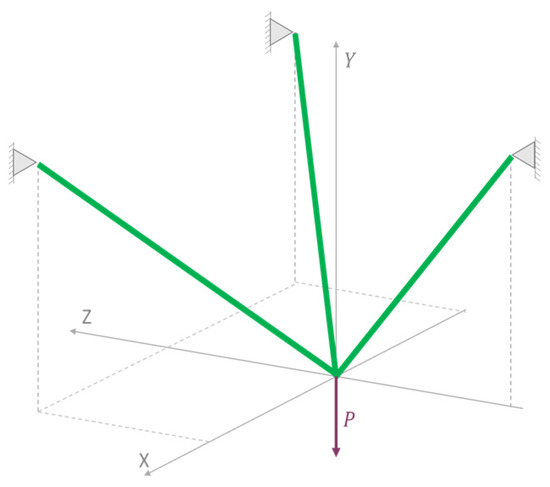
Figure 13.
Schematic representation of three-dimensional structure under downward load.
Table 9 shows the spatial coordinates of the 3D truss supports.
Table 9.
Spatial Coordinates of Three-dimensional Truss’s Simple Supports.
The results obtained for each of the objective functions, are presented in Table 10. The two columns with the exponents ey are respectively related to the minimization of the maximum displacement fmin and the maximization of the fundamental frequency fmax.
Table 10.
Results of the Optimization Study: Minimum Displacement and Maximum Fundamental Frequency for One Design Variable.
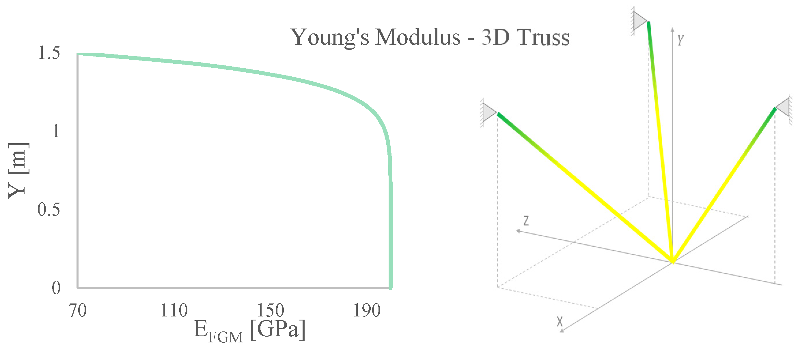
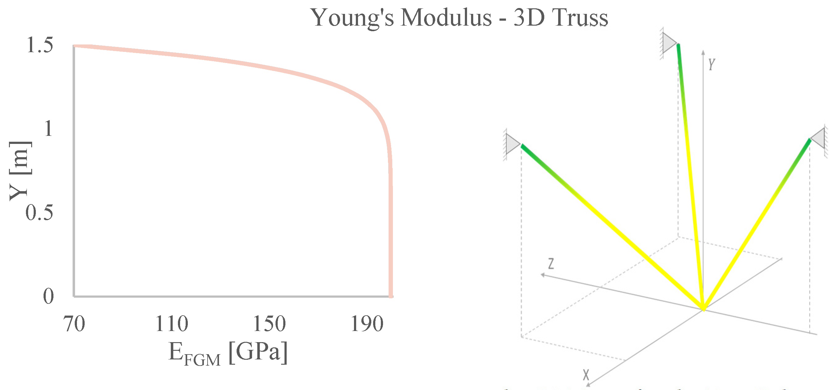
Figure 14 and Figure 15 show the evolution of the modulus of elasticity characterized by the best solution found for minimizing the maximum resultant displacement and for maximizing the fundamental frequency of the 3D truss, respectively. These figures include a schematic representation of the structure’s configuration showing the constituent material mixture of the FGM throughout the structure height.
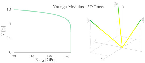
Figure 14.
Evolution of the Young’s Modulus of the 3D Truss for the Best Solution Found for Minimizing the Maximum Resulting Displacement using One Design Variable.

Figure 15.
Evolution of the Young’s Modulus of the 3D Truss for the Best Solution Found for Maximizing the Fundamental Frequency using One Design Variable.
For this structure, it should be noted that for a situation in which the aim is to both minimize the resulting displacements and to maximize the fundamental frequency, the most advantageous distribution of properties is characterized by an exponent 10, in which zirconia makes up the entire structure up to a height of around 0.9 m.
- Case 6—3D Structure II—Optimization
In this study, one considers a 3D frame-type structure as shown in Figure 16. This structure is subjected to optimization processes considering the same objective functions as previous cases. The design variable is also the exponent of the power law volume fraction function. The structure is discretized into 15 beam elements 1 m long (aspect ratio 20) and it is subjected to a concentrated load P = 1000 N in the static case.
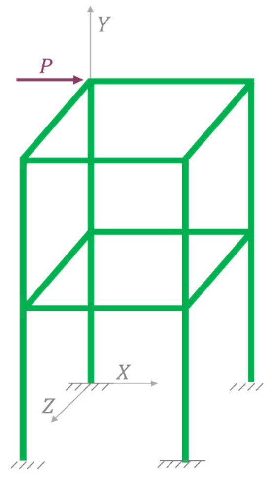
Figure 16.
Three-dimensional Frame.
The results obtained for each objective function are presented in Table 11, where the two columns with the exponents ey are respectively related to the minimization of the maximum displacement fmin and to the maximization of the fundamental frequency fmax.
Table 11.
Results of the Optimization Study of the 3D Frame using RFO with One Design Variable.
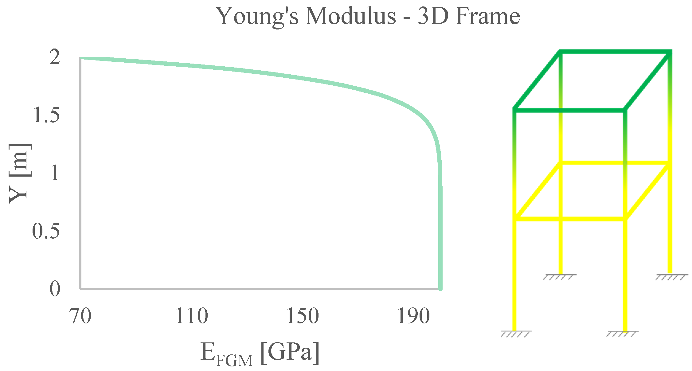
Figure 17 and Figure 18 show the evolution of the modulus of elasticity associated with the best solution found for minimizing the maximum resultant displacement and for maximizing the fundamental frequency of the 3D frame, respectively. These figures include a schematic representation of the structure’s configuration with the evolution of the constituent material mixture throughout the structure height.

Figure 17.
Evolution of the Modulus of Elasticity of the 3D Frame for the Best Solution Found for Minimizing the Maximum Resulting Displacement using One Design Variable.
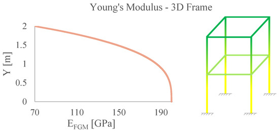
Figure 18.
Evolution of the Young’s Modulus of the 3D Frame for the Best Solution Found for Maximizing Natural Frequency using One Design Variable.
Once again, when the objective is to minimize the resulting displacement, the exponent that enables the best static behaviour of the structure is 10. If the objective function is the maximization of the fundamental frequency, the power law exponent that characterizes the best free vibration behaviour is, for the present structure, approximately 3.2.
6.4. Optimization Case Studies—Four Design Variables
In this subsection the optimization processes the structures will undergo have similar objective functions, but now consider four design variables as described in the Methodology section. Besides the exponent of the power law volume fraction, the next tables consider three additional columns whose acronyms are RM, M1 and M2. RM corresponds to how the rule of mixtures is considered, i.e., if a specific random variable assumes the value 1, the volume fraction characterizes the distribution of metallic material; if it assumes the value 2, then the volume fraction describes the ceramic material distribution. Regarding the acronym M1, this is related to the third design variable which defines the metallic constituent material to be used. The fourth design variable, M2, defines the ceramic material to be used.
- Case 7—2D Frame-type Structure—Optimization
The optimization results for the 2D frame structure previously analyzed with only one design variable, but now considering four design variables, are presented in Table 12 and Table 13. These tables denote respectively the results achieved in the minimization of the maximum resultant displacement and the maximization of the fundamental frequency.
Table 12.
Results of the Optimization Study for 2D Frame using the RFO Algorithm for Four design variables to Minimize the Maximum Resulting Displacement.
Table 13.
Results of the Optimization Study for 2D Frame using RFO for four design variables to Maximize the Fundamental Frequency.
Figure 19 and Figure 20 show the evolution of Young’s modulus through the structure for the best solutions found in both optimization processes.
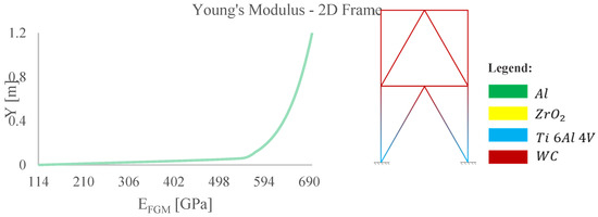
Figure 19.
Evolution of Young’s Modulus of the 2D Frame for the Best Solution found for Minimizing the Maximum Resulting Displacement using four Design Variables.
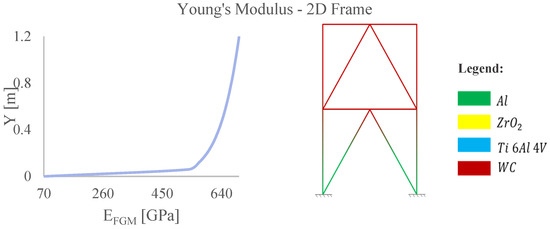
Figure 20.
Evolution of Young’s Modulus of 2D Frame for the Best Solution found for Maximizing Natural Frequency using four Design Variables.
The optimum configuration found with four design variables that yield the lowest maximum resultant displacement corresponds to a frame made of titanium in the lower zone and tungsten carbide in the upper zone, reducing the maximum resultant displacement by around six times. The optimum solution found by the RFO for the fundamental frequency maximization corresponds to the frame made of tungsten carbide in the lower zone and aluminium in the upper zone of the structure, with an exponent of 0.1, and leads to a better solution when compared with the optimal solution using one design variable.
- Case 8—3D Frame-type Structure—Optimization
This case study is the last of this work and considers the 3D frame already analysed in Case 4, but now with a broader perspective considering four design variables. Table 14 and Table 15 show the results obtained in the minimization process of the maximum resultant displacement and the maximization of the fundamental frequency of the 3D frame, respectively.
Table 14.
Results of the Optimization Study of the 3D Frame using RFO for Four Design Variables to Minimize the Maximum Resulting Displacement.
Table 15.
Results of the Optimization Study of the 3D Frame using RFO for Four Design Variables to Maximize the Fundamental Frequency.
Figure 21 and Figure 22 depict the evolution of Young’s modulus for the best solution found for minimizing the maximum resultant displacement and maximizing the fundamental frequency of the 3D frame, respectively, including also schematic representations of the FGM evolution throughout the structure’s height.
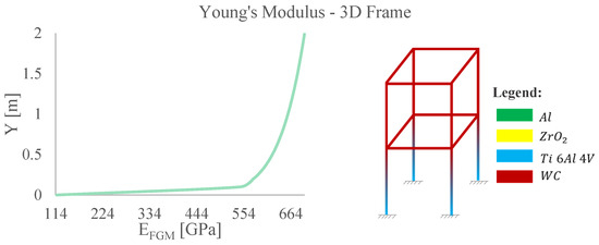
Figure 21.
Evolution of Young’s Modulus of the 3D Frame for the Best Solution for Minimizing the Maximum Resulting Displacement using Four Design Variables.
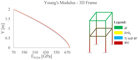
Figure 22.
Evolution of Young’s Modulus of the 3D Frame for the Best Solution Found for Maximizing the Fundamental Frequency using Four Design Variables.
The best solution found for the maximum displacement minimization corresponds to the combination of titanium next to the encasements and tungsten carbide in the upper area of the structure, obtaining a maximum displacement approximately four times lower than the result achieved with one design variable. To maximize the fundamental frequency, the optimum solution obtained with the four design variables corresponds to a combination of tungsten carbide next to the encasements and aluminum in the upper area of the structure, with an exponent of approximately 1.5. This leads to a fundamental frequency around 1.35 times higher than that found with the one-design variable optimization procedure.
7. Conclusions
In the present work, the optimization of a set of 2D and 3D discrete structures was conducted concerning the minimization of the maximum resulting displacement and the maximization of the fundamental frequency, in separate single-objective optimization processes. Only side constraints were considered.
Considering the first stage of the optimization studies where only one design variable was considered, the results achieved make it possible to conclude that, when the objective is the minimization of the maximum resulting displacement, in a situation where the structure is entirely metallic at the highest coordinate and entirely ceramic at the lowest coordinate, the progression between the two materials should correspond to a power law exponent of 10, which provides a stiffer structure. When the objective is to maximize the fundamental frequency, it is not possible to generalize, and it was found that for the 2D truss, the exponent should be approximately 0.18; while for the 2D frame, the best solution corresponds to an exponent of approximately 1.4. For the 3D truss it should be 10 and, for the 3D frame, the best solution found corresponds to an exponent of approximately 1.5.
When four design variables are considered, the benefits achieved in terms of reducing the resultant displacements are clear, in some cases very significantly, and in the frequencies’ increase for most cases as seen during the cases’ presentation. These improvements are possible through the optimal combination and distribution of the different materials, along with the exponent values assumed; however, it should not be generalized optimal solutions for all structures, as each structure should be considered on a case-by-case basis.
It is worth noting, the good performance of the implemented metaheuristic optimization technique and its coupling with the finite element method for FGM structures’ optimization.
Also pertinent to say that, even if a set of other non-functionally graded materials, such as isotropic and homogeneous materials are to be used in building the analysed structures, the present results can provide insightful indications about the disposition of such materials’ constant propertiesalong the structure’s height, for nearly optimized responses.
Following the promising optimal solutions found, will be relevant to pursue further optimization studies, considering a multiobjective approach for behavioural-constrained problems.
Author Contributions
Conceptualisation, M.A.R.L. and J.I.B. software, J.S.D.G. and M.A.R.L. formal analysis, J.S.D.G., M.A.R.L. and J.I.B. data curation, J.S.D.G. writing—original draft preparation, J.S.D.G. writing—review and editing, J.S.D.G., M.A.R.L. and J.I.B. visualisation, J.S.D.G. supervision, M.A.R.L. and J.I.B. All authors have read and agreed to the published version of the manuscript.
Funding
This research received no external funding.
Data Availability Statement
The data generated or analysed are in the manuscript itself.
Acknowledgments
The authors acknowledge the support by FCT, through IDMEC, under LAETA, project UIDB/50022/2020.
Conflicts of Interest
The authors declare no conflicts of interest.
Appendix A
Table A1.
The complete set of 100 runs conducted for the second verification case.
Table A1.
The complete set of 100 runs conducted for the second verification case.
| Run | fmin | Run | fmin | Run | fmin | Run | fmin |
|---|---|---|---|---|---|---|---|
| 1 | 1.4522 × 10⁻⁸ | 26 | 2.4419 × 10⁻⁸ | 51 | 2.2693 × 10⁻⁷ | 76 | 3.0780 × 10⁻⁸ |
| 2 | 1.5391 × 10⁻¹⁰ | 27 | 2.1011 × 10⁻⁶ | 52 | 4.3243 × 10⁻¹⁰ | 77 | 2.0209 × 10⁻¹⁰ |
| 3 | 3.8610 × 10⁻⁷ | 28 | 5.2479 × 10⁻⁹ | 53 | 3.4839 × 10⁻¹⁰ | 78 | 2.0575 × 10⁻⁸ |
| 4 | 2.5061 × 10⁻¹⁰ | 29 | 3.4899 × 10⁻⁸ | 54 | 1.7969 × 10⁻⁶ | 79 | 5.4393 × 10⁻⁸ |
| 5 | 9.6072 × 10⁻⁹ | 30 | 2.1826 × 10⁻⁷ | 55 | 1.5886 × 10⁻⁹ | 80 | 1.2861 × 10⁻⁹ |
| 6 | 1.0757 × 10⁻⁸ | 31 | 1.0316 × 10⁻⁶ | 56 | 4.3608 × 10⁻⁷ | 81 | 1.2005 × 10⁻⁷ |
| 7 | 1.1787 × 10⁻⁸ | 32 | 1.0324 × 10⁻⁸ | 57 | 5.3363 × 10⁻⁷ | 82 | 5.4759 × 10⁻⁷ |
| 8 | 2.3982 × 10⁻⁹ | 33 | 1.5102 × 10⁻⁹ | 58 | 3.9452 × 10⁻⁹ | 83 | 1.9531 × 10⁻⁷ |
| 9 | 6.9128 × 10⁻⁹ | 34 | 4.4206 × 10⁻⁷ | 59 | 1.4520 × 10⁻⁷ | 84 | 1.1211 × 10⁻⁸ |
| 10 | 3.0236 × 10⁻⁷ | 35 | 1.8854 × 10⁻⁸ | 60 | 1.7240 × 10⁻⁸ | 85 | 2.7878 × 10⁻¹⁰ |
| 11 | 8.3510 × 10⁻⁹ | 36 | 1.6673 × 10⁻⁸ | 61 | 6.4870 × 10⁻⁷ | 86 | 6.8652 × 10⁻⁷ |
| 12 | 4.2426 × 10⁻¹¹ | 37 | 7.7937 × 10⁻¹⁰ | 62 | 1.5427 × 10⁻⁸ | 87 | 4.2135 × 10⁻⁹ |
| 13 | 1.1228 × 10⁻⁷ | 38 | 1.2790 × 10⁻¹⁰ | 63 | 8.1588 × 10⁻⁹ | 88 | 1.1548 × 10⁻⁷ |
| 14 | 5.5395 × 10⁻⁷ | 39 | 9.6050 × 10⁻⁹ | 64 | 2.8892 × 10⁻¹¹ | 89 | 4.2666 × 10⁻⁸ |
| 15 | 9.7326 × 10⁻⁹ | 40 | 1.9212 × 10⁻⁶ | 65 | 2.6553 × 10⁻⁸ | 90 | 3.5685 × 10⁻⁸ |
| 16 | 8.1542 × 10⁻⁹ | 41 | 1.1275 × 10⁻⁸ | 66 | 3.0041 × 10⁻⁸ | 91 | 9.1252 × 10⁻⁸ |
| 17 | 2.2786 × 10⁻⁷ | 42 | 7.4339 × 10⁻⁷ | 67 | 6.5576 × 10⁻⁷ | 92 | 3.1998 × 10⁻¹⁰ |
| 18 | 1.4118 × 10⁻¹¹ | 43 | 2.2533 × 10⁻⁷ | 68 | 3.5742 × 10⁻⁹ | 93 | 1.2050 × 10⁻⁹ |
| 19 | 9.3447 × 10⁻⁸ | 44 | 1.2538 × 10⁻⁷ | 69 | 6.6478 × 10⁻⁸ | 94 | 1.6008 × 10⁻¹⁰ |
| 20 | 4.3996 × 10⁻⁷ | 45 | 3.6096 × 10⁻⁹ | 70 | 7.8763 × 10⁻¹¹ | 95 | 3.9891 × 10⁻⁸ |
| 21 | 1.2128 × 10⁻⁸ | 46 | 7.1873 × 10⁻¹⁰ | 71 | 3.1665 × 10⁻⁸ | 96 | 4.4292 × 10⁻⁸ |
| 22 | 5.5121 × 10⁻⁹ | 47 | 4.2522 × 10⁻¹⁰ | 72 | 7.5925 × 10⁻⁹ | 97 | 5.8937 × 10⁻⁸ |
| 23 | 4.6802 × 10⁻¹⁰ | 48 | 1.2298 × 10⁻⁷ | 73 | 7.1936 × 10⁻⁸ | 98 | 9.8581 × 10⁻⁸ |
| 24 | 8.2569 × 10⁻¹⁰ | 49 | 2.2679 × 10⁻¹⁰ | 74 | 4.9475 × 10⁻¹⁰ | 99 | 2.0966 × 10⁻¹⁰ |
| 25 | 1.2069 × 10⁻⁸ | 50 | 4.2401 × 10⁻¹⁰ | 75 | 1.0763 × 10⁻¹¹ | 100 | 1.0812 × 10⁻¹⁰ |
| Present average value | 1.6230 × 10⁻⁷ | ||||||
| Average value [22] | 7.5400 × 10⁻⁸ | ||||||
| Present standard deviation | 3.7069 × 10⁻⁷ | ||||||
| Standard deviation [22] | 2.7800 × 10⁻⁸ | ||||||
References
- Reddy, J.N. Analysis of functionally graded plates. Int. J. Numer. Methods Eng. 2000, 47, 663–684. [Google Scholar] [CrossRef]
- Maalawi, K. Optimization of Functionally Graded Material Structures: Some Case Studies. In Optimum Composite Structures; IntechOpen: London, UK, 2019. [Google Scholar] [CrossRef]
- Loja, M.A.R.; Barbosa, J.I.; Soares, C.M.M. A study on the modeling of sandwich functionally graded particulate composites. Compos. Struct. 2012, 94, 2209–2217. [Google Scholar] [CrossRef]
- Pasha, A.; Rajaprakash, B.M. Functionally graded materials (FGM) fabrication and its potential challenges & applications. Mater. Today Proc. 2021, 52, 413–418. [Google Scholar] [CrossRef]
- Markworth, A.J.; Saunders, J.H. A model of structure optimization for a functionally graded material. Mater. Lett. 1995, 22, 103–107. [Google Scholar] [CrossRef]
- Gasik, M.M. Micromechanical modelling of functionally graded materials. Comput. Mater. Sci. 1998, 13, 42–55. [Google Scholar] [CrossRef]
- Chalal, H.; Abed-Meraim, F. Quadratic Solid–Shell Finite Elements for Geometrically Nonlinear Analysis of Functionally Graded Material Plates. Materials 2018, 11, 1046. [Google Scholar] [CrossRef]
- Elishakoff, I.; Pentaras, D.; Gentilini, C. Mechanics of Functionally Graded Material Structures; World Scientific Pub Co. Pte Ltd.: Singapore, 2015. [Google Scholar]
- Wang, W.; Yuan, H.; Li, X.; Shi, P. Stress Concentration and Damage Factor Due to Central Elliptical Hole in Functionally Graded Panels Subjected to Uniform Tensile Traction. Materials 2019, 12, 422. [Google Scholar] [CrossRef]
- Sayyad, A.S.; Ghugal, Y.M. Bending, buckling and free vibration of laminated composite and sandwich beams: A critical review of literature. Compos. Struct. 2017, 171, 486–504. [Google Scholar] [CrossRef]
- Loja, M.R.; Soares, C.M. Modelling and design of adaptive structures using B-spline strip models. Compos. Struct. 2002, 57, 245–251. [Google Scholar] [CrossRef]
- Loja, M.A.R.; Soares, C.M.M.; Soares, C.A.M. Higher-order B-spline finite strip model for laminated adaptive structures. Compos. Struct. 2001, 52, 419–427. [Google Scholar] [CrossRef]
- Zhang, N.; Khan, T.; Guo, H.; Shi, S.; Zhong, W.; Zhang, W. Functionally Graded Materials: An Overview of Stability, Buckling, and Free Vibration Analysis. Adv. Mater. Sci. Eng. 2018, 2019, 1–18. [Google Scholar] [CrossRef]
- Mota, A.F.; Loja, M.A.R.; Barbosa, J.I.; Rodrigues, J.A. Porous Functionally Graded Plates: An Assessment of the Influence of Shear Correction Factor on Static Behavior. Math. Comput. Appl. 2020, 25, 25. [Google Scholar] [CrossRef]
- Neves, A.M.A.; Ferreira, A.; Carrera, E.; Cinefra, M.; Roque, C.; Jorge, R.M.N.; Soares, C.M.M. Static, free vibration and buckling analysis of isotropic and sandwich functionally graded plates using a quasi-3D higher-order shear deformation theory and a meshless technique. Compos. Part B Eng. 2013, 44, 657–674. [Google Scholar] [CrossRef]
- Loja, M.A.R.; Barbosa, J.I.; Soares, C.M.M. Dynamic behaviour of soft core sandwich beam structures using kriging-based layerwise models. Compos. Struct. 2015, 134, 883–894. [Google Scholar] [CrossRef]
- Merdaci, S.; Adda, H.M.; Hakima, B.; Dimitri, R.; Tornabene, F. Higher-Order Free Vibration Analysis of Porous Functionally Graded Plates. J. Compos. Sci. 2021, 5, 305. [Google Scholar] [CrossRef]
- Ergun, A.; Yu, X.; Valdevit, A.; Ritter, A.; Kalyon, D.M. Radially and Axially Graded Multizonal Bone Graft Substitutes Targeting Critical-Sized Bone Defects from Polycaprolactone/Hydroxyapatite/Tricalcium Phosphate. Tissue Eng. Part A 2012, 18, 2426–2436. [Google Scholar] [CrossRef]
- Muhammed, S.A.; Al-Khafaji, A.M.; Al-Deen, H.H.J.J. The Influence of Strontium Oxide on the Physio-Mechanical Properties of Biomedical-Grade Titanium in Ti-SrO Composites. J. Compos. Sci. 2023, 7, 449. [Google Scholar] [CrossRef]
- Yeslam, H.E. Flexural Behavior of Biocompatible High-Performance Polymer Composites for CAD/CAM Dentistry. J. Compos. Sci. 2023, 7, 270. [Google Scholar] [CrossRef]
- Hashim, F.A.; Hussain, K.; Houssein, E.H.; Mabrouk, M.S.; Al-Atabany, W. Archimedes optimization algorithm: A new metaheuristic algorithm for solving optimization problems. Appl. Intell. 2020, 51, 1531–1551. [Google Scholar] [CrossRef]
- Połap, D.; Woźniak, M. Red fox optimization algorithm. Expert Syst. Appl. 2020, 166, 114107. [Google Scholar] [CrossRef]
- Braik, M.S. Chameleon Swarm Algorithm: A bio-inspired optimizer for solving engineering design problems. Expert Syst. Appl. 2021, 174, 114685. [Google Scholar] [CrossRef]
- Nikbakht, S.; Kamarian, S.; Shakeri, M. A review on optimization of composite structures Part II: Functionally graded materials. Compos. Struct. 2019, 214, 83–102. [Google Scholar] [CrossRef]
- Birman, V.; Byrd, L.W. Modeling and Analysis of Functionally Graded Materials and Structures. Appl. Mech. Rev. 2007, 60, 195–216. [Google Scholar] [CrossRef]
- Santos, J.; Sohouli, A.; Suleman, A. Micro- and Macro-Scale Topology Optimization of Multi-Material Functionally Graded Lattice Structures. J. Compos. Sci. 2024, 8, 124. [Google Scholar] [CrossRef]
- Loja, M.A.R. On the use of particle swarm optimization to maximize bending stiffness of functionally graded structures. J. Symb. Comput. 2014, 61–62, 12–30. [Google Scholar] [CrossRef]
- Wu, C.-P.; Li, K.-W. Multi-Objective Optimization of Functionally Graded Beams Using a Genetic Algorithm with Non-Dominated Sorting. J. Compos. Sci. 2021, 5, 92. [Google Scholar] [CrossRef]
- Jaszcz, A.; Połap, D.; Damaševičius, R. Lung X-ray Image Segmentation Using Heuristic Red Fox Optimization Algorithm. Sci. Program. 2022, 2022, 1–8. [Google Scholar] [CrossRef]
- Bhuvaneshwari, M.; Kanaga, E.G.M.; Anitha, J. Bio-inspired Red Fox-Sine cosine optimization for the feature selection of SSVEP-based EEG signals for BCI applications. Biomed. Signal Process. Control. 2023, 80. [Google Scholar] [CrossRef]
- Gopi, P.S.S.; Karthikeyan, M. Red fox optimization with ensemble recurrent neural network for crop recommendation and yield prediction model. Multimedia Tools Appl. 2023, 83, 13159–13179. [Google Scholar] [CrossRef]
- Bamikole, J.O.; Narasigadu, C. Application of Pathfinder, Honey Badger, Red Fox and Horse Herd algorithms to phase equilibria and stability problems. Fluid Phase Equilibria 2023, 566. [Google Scholar] [CrossRef]
- Zhang, M.; Xu, Z.; Lu, X.; Liu, Y.; Xiao, Q.; Taheri, B. An optimal model identification for solid oxide fuel cell based on extreme learning machines optimized by improved Red Fox Optimization algorithm. Int. J. Hydrogen Energy 2021, 46, 28270–28281. [Google Scholar] [CrossRef]
- Gaspar, J.S.D.; Loja, M.A.R.L.; Barbosa, J.I. Static and Free Vibration Analyses of Functionally Graded Plane Structures. J. Compos. Sci. 2023, 7, 377. [Google Scholar] [CrossRef]
- Mohammed, H.; Rashid, T. FOX: A FOX-inspired optimization algorithm. Appl. Intell. 2023, 53, 1030–1050. [Google Scholar] [CrossRef]
- Reddy, J.N. Mechanics of Laminated Composite Plates and Shells: Theory and Analysis; CRC Press: Boca Raton, FL, USA, 2004. [Google Scholar]
- Loja, M.A.R.; Rzeszut, K.; Barbosa, J.I. Nonlocal Free Vibrations of Metallic FGM Beams. J. Compos. Sci. 2022, 6, 125. [Google Scholar] [CrossRef]
- Luo, Y. An efficient 3D Timoshenko beam element with consistant shape functions An Efficient 3D Timoshenko Beam Element with Consistent Shape Functions. Adv. Theor. Appl. Mech. 2008, 1, 95–106. Available online: https://www.researchgate.net/publication/259345543 (accessed on 7 March 2023).
- Bazoune, A.; Khulief, Y.; Stephen, N. Shape functions of three-dimensional timoshenko beam element. J. Sound Vib. 2003, 259, 473–480. [Google Scholar] [CrossRef]
- Sasa, G. Development of a New 3D Beam Finite Element with Deformable Section. Ph.D. Thesis, Université de Lyon, Lyon, France, 2017. Available online: http://theses.insa-lyon.fr/publication/2017LYSEI026/these.pdf (accessed on 5 March 2023).
- Gherlone, M.; Cerracchio, P.; Mattone, M.; Di Sciuva, M.; Tessler, A. Shape sensing of 3D frame structures using an inverse Finite Element Method. Int. J. Solids Struct. 2012, 49, 3100–3112. [Google Scholar] [CrossRef]
- Khebizi, M.; Guenfoud, H.; Guenfoud, M.; El Fatmi, R. Three-dimensional modelling of functionally graded beams using Saint-Venant’s beam theory. Struct. Eng. Mech. 2019, 72, 257–273. [Google Scholar] [CrossRef]


Disclaimer/Publisher’s Note: The statements, opinions and data contained in all publications are solely those of the individual author(s) and contributor(s) and not of MDPI and/or the editor(s). MDPI and/or the editor(s) disclaim responsibility for any injury to people or property resulting from any ideas, methods, instructions or products referred to in the content. |
© 2024 by the authors. Licensee MDPI, Basel, Switzerland. This article is an open access article distributed under the terms and conditions of the Creative Commons Attribution (CC BY) license (https://creativecommons.org/licenses/by/4.0/).