


Abstract
Evaluating conditional time-series generation models remains challenging in battery research, where degradation data are often limited and experiments cover only a small number of operating conditions. The widely used Fréchet Inception Distance (FID) summarizes all conditions into a single score, which can obscure failures under rare but safety-critical conditions. Several condition-aware extensions of FID, including Conditional Fréchet Inception Distance (CFID), partially address this limitation by evaluating each condition separately. However, these approaches do not assess whether physically meaningful relationships between operating conditions are preserved, and their reliability deteriorates when only a few samples are available for each condition. To address these issues, we propose a three-layer diagnostic framework for evaluating conditional generative models under limited-data conditions. The first layer, Stratified Fréchet Distance, identifies the specific operating conditions and degradation phases where generation quality degrades. The second layer, based on Conditional Response Consistency (CRC), Conditional Distance Ratio (CDR), and Mean-Order Preservation (MOP), evaluates whether the model preserves the distance structure and ordering between conditions. MOP detects condition-ordering defects that CRC cannot identify when the real data distance matrix is non-monotone. This layer also enables statistically meaningful comparisons even when only a small number of samples are available. The third layer detects strata where statistical estimates are unreliable and provides a more stable alternative for evaluation. We validate the framework on four battery degradation datasets using two generative model architectures. The proposed approach reveals condition-specific failures that are not captured by conventional FID. It localizes generation errors to the late-stage high-temperature degradation regime that is most relevant to battery safety. The framework also detects structural distortions with statistical significance. In addition, it consistently ranks physics-informed model variants across quality differences spanning seven orders of magnitude. These results demonstrate that the proposed framework provides a practical and physically interpretable evaluation methodology for conditional generative modeling in battery degradation analysis.
1. Introduction
The safety of lithium-ion batteries depends critically on operating temperature. High temperatures accelerate SEI (solid electrolyte interphase, a passivation layer that forms on the anode surface) growth and cathode decomposition, increasing the risk of thermal runaway (uncontrolled exothermic reaction) [1]. Low temperatures promote lithium plating (metallic lithium deposition on the anode) and dendrite-driven internal short circuits [2]. Quantitative characterization of degradation across all operating conditions is a prerequisite for safety assessment [3].
Yet, experimental data under the extreme conditions most critical for safety—high or low temperature, high C-rate (the ratio of charge/discharge current to battery capacity)—are costly to acquire and inevitably underrepresented in existing datasets [4,5]. Deep generative models [6,7,8,9] have advanced to the point where synthesizing degradation curves for such conditions is becoming feasible [10,11,12,13,14]. In the emerging paradigm of battery digital twins [15,16], synthetic data are already used to augment limited experiments and simulate untested scenarios. A digital twin maintains a virtual replica of a physical battery system, continuously updated with sensor data, and uses generative models to predict degradation under conditions not yet encountered in service—for example, forecasting capacity fade at temperatures outside the tested range or under novel charge protocols. The fidelity of such predictions depends directly on the quality of the underlying generative model at each operating condition. As safety decisions increasingly rely on such data, their trustworthiness becomes a practical engineering concern.
Evaluating synthetic degradation data, however, requires answering two distinct questions that current metrics conflate or ignore. The first is per-condition quality: does the generative model produce accurate curves at each temperature and in each degradation phase? The second is inter-condition structural consistency: does the model preserve the physical relationships across conditions—for example, the monotonic acceleration of degradation from 25 °C to 43 °C?
These questions are difficult to answer because battery degradation data possess three characteristics that set them apart from the large-scale image datasets for which evaluation metrics such as FID were designed.
First, the data are scarce. Battery datasets typically contain tens to at most a few hundred cells [4,5], in contrast to the tens of thousands of samples available for image generation. Per-condition evaluation must therefore work reliably with extremely limited samples—a regime in which covariance-based metrics become statistically unstable.
Second, physical conditions induce qualitative changes in the degradation trajectory. Changing the temperature from 25 °C to 43 °C changes the dominant degradation mechanism (e.g., from gradual SEI thickening to rapid electrolyte decomposition), producing curves with qualitatively different shapes and lifetimes [3]. Similar condition-dependent changes arise in other physics-governed domains, such as rotating machinery fault diagnosis [17] and materials processing [18].
Third, the most important conditions are the rarest. Extreme temperatures and high C-rates are most relevant to safety yet most expensive to test. Mayer et al. [19] have shown that generative models trained by maximum likelihood inherently under-represent such minorities, making quality evaluation under these conditions doubly important.
The standard metric, Fréchet Inception Distance (FID) [20], addresses none of these challenges. It aggregates all data into a single scalar, and its feature space has been shown to mask quality differences even when they are perceptually apparent [21]. CFID [22] and Fréchet Joint Distance (FJD) [23] evaluate per-condition quality for discrete image classes. Neither addresses temporal diagnosis or confounding detection, which require stratification along additional axes. Neither assesses whether the generative model preserves the physical relationships between conditions—a question that calls for a dedicated structural verification step. And neither accounts for the statistical unreliability of covariance-based estimates when only a handful of samples are available per condition.
Consider a model that generates good 25 °C curves but poor 43 °C curves (12% of the dataset; Figure 1). FID dilutes the 43 °C failure into the 88% of the correct samples and remains virtually unchanged. Dilution also occurs along the temporal axis: battery degradation proceeds through linear fade followed by nonlinear acceleration beyond the knee point (the inflection where capacity fade transitions from gradual to rapid) [24], and FID lets early-phase success mask late-phase failure. Even if a model generates plausible curves at each temperature individually, it may distort the relative distances between conditions—producing 43 °C curves that look more like 25 °C than they should. Neither FID nor CFID can detect this structural distortion.
Figure 1.
Temperature-dependent capacity degradation curves from the NASA battery dataset [25]. Degradation rate and pattern vary substantially across temperatures. Accurate reproduction of minority-condition behavior (43 °C, 44 °C) is a prerequisite for safety evaluation. The remaining three datasets (SNL, MICH, CALB) used in this study are from the BatteryLife benchmark [26].
To address these challenges, we propose a three-layer diagnostic framework. The first layer, Stratified Fréchet Distance (SFD), partitions data by operating condition, temporal segment, or both, and diagnoses where and when generation quality breaks down. SFD with reduces exactly to CFID and is adopted as the default. Inter-condition consistency, previously addressed by the Between-SFD term (), is now handled more directly by the second layer. The second layer introduces two new metrics for inter-condition structural verification: Conditional Response Consistency (CRC) for datasets with three or more conditions, and Conditional Distance Ratio (CDR) for datasets with only two. Both measure whether the generative model preserves the distance structure between conditions, and permutation tests provide statistical significance. The third layer addresses reliability under data scarcity: Effective Stratum Size (ESS) flags strata where Fréchet distance estimation is unreliable, and Stratified MMD (S-MMD) provides a covariance-free alternative for such strata.
We validate the framework on four battery datasets (NASA [25], SNL, MICH, CALB [26], 161 cells in total) with conditional VAE and conditional Flow Matching [27] models. The experiments reveal that SFD identifies per-condition quality degradation that FID entirely misses. In a controlled experiment where a model is trained on a single temperature, FID remains virtually unchanged from the baseline, whereas SFD reveals that the excluded conditions are nearly twice as far from reality as the training condition. Condition-by-time stratification further localizes the largest quality gap to the late degradation phase at 35 °C, the regime most relevant to safety. The structural verification layer confirms that well-trained generators preserve the physical ordering of inter-condition distances while deficient generators distort it. A CRC permutation test on cross-stratified condition pairs achieves statistical significance () for temperature–C-rate structured data. MOP detects condition-ordering defects across four battery datasets with 100% detection rate on three datasets (, ). CDR extends this structural verification to datasets with only two conditions, reliably distinguishing normal from distorted generation with bootstrap confidence intervals. These findings hold across all four datasets and across two fundamentally different generative architectures (CVAE and conditional Flow Matching with Fourier Neural Operator).
This work makes four contributions. First, we characterize three properties of physics-governed time series generation—data scarcity, condition-dependent qualitative changes, and minority-condition importance—that make evaluation fundamentally different from large-scale image generation and that existing metrics do not address. Second, we propose a three-layer diagnostic framework comprising SFD for per-condition quality diagnosis; CRC, CDR, and MOP for inter-condition structural verification with statistical significance; and ESS and S-MMD for small-sample reliability assessment. CRC and CDR are motivated by Benny et al.’s between-class evaluation [28] and extend it by testing rank ordering and distance magnitude preservation with formal permutation tests. MOP is a new indicator that detects condition-ordering defects (type-2 inversion and type-3 confusion) when CRC lacks power due to small K or non-monotone real data. Third, we analyze the detection power of Fréchet distance and MMD in the small-sample regime, derive the optimal feature dimension , and establish the complementarity regime in which MMD-based evaluation becomes preferable to FD-based evaluation. Fourth, we validate the framework through fourteen experiments across four datasets, three feature extractors, and two generative architectures, confirming that the diagnostic capabilities are robust to the choice of data source, feature space, and generative model. Experiments 1–9 validate Layer 1. Experiment 10 introduces and validates MOP for Layer 2. Experiments 11–14, reported in Appendix C, provide detailed Layer 2 validation covering seed dependence, cross-dataset generalization, CRC minimum-K requirements, and CDR inflation conditions. The experiments demonstrate increased diagnostic sensitivity under controlled failure scenarios, rather than an improvement in generative model performance.
The remainder of this paper is structured as follows. Section 2 reviews the background on conditional time series generation and formalizes the dilution problem. Section 3 presents the three-layer diagnostic framework in detail: Layer 1 (SFD and its stratification variants), Layer 2 (CRC and CDR for structural verification), and Layer 3 (ESS and S-MMD for reliability assessment). Section 4 and Section 5 describe the experimental setup and report results. Section 6 discusses the implications of the findings and their limitations. Section 7 concludes the paper.
2. Background
2.1. Conditional Time Series Generation
A conditional time series generation model receives a condition parameter c (e.g., temperature or C-rate) and learns the conditional distribution of the time series x. The paradigm originated in image synthesis with Conditional GANs [29] and Conditional VAEs [30], and has since been extended through classifier-free guidance [31] and Conditional Flow Matching [9].
Adaptation to time series has proceeded along several lines. TimeGAN [11] introduced an embedding network to capture temporal dynamics. TimeVAE [12] proposed a VAE architecture tailored to a sequential structure. CSDI [13] applied conditional score-based diffusion to time series imputation. In the battery domain, DiffBatt [14] demonstrated that conditional generation of degradation curves can be combined with lifetime prediction for practical data augmentation.
These advances make it increasingly feasible to synthesize degradation curves under conditions for which no experimental data exist. Beyond data augmentation, conditional generation enables scenario analysis—synthesizing degradation trajectories under hypothetical operating conditions (e.g., a temperature profile not tested in the laboratory) to support design decisions and safety certification [1]. The value of such scenario generation depends entirely on the fidelity of the generated data at each target condition, making per-condition quality evaluation a prerequisite for any downstream use.
2.2. The Fréchet Inception Distance and Its Limitations
FID [20] is the standard metric for evaluating generative models. It fits Gaussian distributions to the features of real and generated data and computes their Fréchet distance:
where and are the mean and covariance of the real and generated feature distributions, respectively.
FID models all data as a single Gaussian. It does not distinguish which operating condition a sample belongs to or which temporal segment of a time series it represents. For homogeneous data, this approximation is acceptable. For battery degradation curves, where distributions differ qualitatively across temperatures, fitting a single Gaussian to the mixture is itself a poor modeling choice.
When FID is applied to time series, domain-specific feature extractors such as InceptionTime [32] replace the Inception network used in image generation [33]. Changing the feature extractor, however, does not alter the structural limitation: FID aggregates a mixture distribution into a single scalar. Stein et al. [21] have further shown that the Inception-V3 feature space can fail to reflect the perceptual quality of generated samples. The limitation we address is more fundamental: it originates not in the choice of feature extractor but in the manner of aggregation itself.
Several conditional evaluation metrics have been proposed. CFID [22] computes FID separately for each class label and averages the results. FJD [23] evaluates the joint distribution of images and conditions. FPD [34] targets physical simulation data. All of these assume discrete class labels (e.g., “dog” or “cat”) and large sample sizes per class. Their extension to continuous physical parameters, temporal quality diagnosis, inter-condition structural verification, confounding detection, and the small-sample regime has not been investigated.
2.3. The Dilution Problem
To formalize FID’s limitation, consider K conditions with data proportions . Suppose a generative model fails only under condition while producing perfect output elsewhere. Because FID evaluates the mixture distribution, the contribution of the failed condition is weighted by its proportion:
Two consequences follow. First, when (e.g., 43 °C constitutes 12% of the dataset), a complete failure at that condition contributes only 12% to FID: this is condition-axis dilution. The rarer a condition, the more severely its failures are diluted—yet rare conditions are precisely those most relevant to safety.
Second, dilution is not confined to the condition axis. Along the temporal axis, a failure in the late degradation phase can be diluted by success in the early phase. When multiple condition parameters are confounded (e.g., temperature and C-rate), evaluating by one variable alone allows the effect of the other to leak into the assessment.
All of these problems stem from pooling subsets with fundamentally different characteristics and evaluating them without distinction. In classical statistics, stratified sampling addresses exactly this situation by respecting the internal structure of the population. The three-layer diagnostic framework proposed in the next section applies this principle to generative model evaluation. Layer 1 (SFD) resolves dilution through stratification. Layer 2 (CRC and CDR) addresses inter-condition structural verification. Layer 3 (ESS and S-MMD) manages statistical reliability under data scarcity.
3. Proposed Diagnostic Framework for Conditional Generation Quality
Evaluating conditional generation quality under data scarcity requires answering three distinct questions, each demanding its own analytical tool. The first question is where and when quality breaks down across operating conditions and degradation phases. The second is whether the generative model preserves the physical relationships that link one condition to another—for instance, the monotonic acceleration of degradation from moderate to high temperatures. The third is how reliable the per-stratum estimates are when some conditions contain as few as three or four batteries.
We organize the framework into three corresponding layers (Table 1). Layer 1 provides per-condition and per-time-segment quality diagnosis through Stratified Fréchet Distance (SFD). Layer 2 introduces Conditional Response Consistency (CRC) and Conditional Distance Ratio (CDR) to verify that the inter-condition distance structure is preserved, with permutation tests [35] supplying statistical significance. Mean-Order Preservation (MOP) is also introduced in Layer 2 to detect condition-ordering defects (type-2 inversion and type-3 confusion) when CRC lacks statistical power due to small K or non-monotone real data distance matrices. Validation is reported in Experiment 10 (Section 5) and Experiments 11–14 (Appendix C). Layer 3 equips the practitioner with Effective Stratum Size (ESS) and Stratified MMD (S-MMD) to assess estimation reliability and to obtain stable alternatives when Fréchet distance estimates are unreliable.
Table 1.
Overview of the diagnostic framework.
The three layers are designed to be used in sequence. A practitioner begins by computing SFD to identify problematic conditions and time segments (Layer 1). The next step is to apply CRC or CDR to determine whether the inter-condition structure is intact (Layer 2). Finally, ESS and S-MMD are consulted to judge which Layer 1 estimates can be trusted and which require caution (Layer 3). If the permutation test in Layer 2 fails to achieve significance because the number of conditions K is small, cross-stratification along a second axis (e.g., temperature × time) increases the number of condition pairs and thereby improves statistical power. If per-stratum sample sizes are below ten, the mean-vector Euclidean distance should replace MMD in the Layer 2 computation to avoid kernel bandwidth instability.
3.1. Layer 1: Quality Diagnosis—Stratified Fréchet Distance (SFD)
The root cause of the dilution problem identified in Section 2 is that FID computes a single distance over the pooled data, allowing failures at minority conditions to be absorbed by the majority. SFD resolves this by partitioning data into strata according to a stratification variable s and computing the Fréchet distance independently within each stratum:
where is the set of strata, denotes the Fréchet distance, and controls the weight of the overall distributional consistency term. Within-SFD assigns equal weight to every stratum, ensuring that a minority condition comprising 6% of the data receives the same attention as one comprising 40%. This equal-weight design is deliberate. A failure at 43 °C is no less consequential than a failure at 4 °C simply because fewer batteries were tested at that temperature. Weighting each stratum by its sample proportion would reproduce precisely the dilution that SFD is designed to avoid. When domain knowledge suggests that certain conditions are more important than others, a weighted average with user-specified weights can be substituted without altering the framework. When , the formulation reduces exactly to CFID [22]. Between-SFD (the term) is the Fréchet distance over the entire mixture distribution, identical to FID. Setting previously served to assess inter-condition distributional consistency alongside per-condition quality. In the present framework, this role is handled more directly and with statistical significance by Layer 2 (CRC and CDR), and is therefore adopted as the recommended default.
The choice of stratification variable determines the diagnostic question that SFD answers (Table 2). Stratification by operating condition (SFDc) reveals which conditions exhibit poor generation quality. Stratification by temporal segment (SFDt) reveals in which phase of the degradation curve the model fails, distinguishing, for example, early linear fade from late nonlinear acceleration beyond the knee point [24]. A failure pattern in which the generative model reproduces the early phase correctly but fails in the late phase is difficult to detect with FID or SFDc, both of which compute features over the entire curve. SFDt detects this failure directly as an elevated Fréchet distance in the late-segment stratum. Stratification by condition×time () provides the finest granularity and can localize a failure to a specific condition in a specific degradation phase. Stratification by multiple condition parameters () exposes inter-condition confounding.
Table 2.
Stratification variables of SFD and their diagnostic roles.
To quantify confounding between two conditioning variables, we define the Confounding Index (CI) as the ratio of SFD computed at a finer stratification granularity to SFD at a coarser one:
A value of CI close to unity indicates that adding the second variable does not materially change the evaluation, implying little confounding. A value exceeding unity indicates that the finer stratification has exposed quality problems hidden at the coarser level, providing a concrete recommendation for which variables to include in model conditioning. CI thus serves not only as a post-hoc evaluation tool but also as an upstream design guide. A CI substantially above unity signals that the omitted conditioning variable should be incorporated into the generative model.
3.2. Layer 2: Structure Verification—CRC and CDR
Layer 1 diagnoses quality within each condition but does not assess whether the generative model preserves the relative distances between conditions. A model might produce plausible curves at each temperature yet compress or invert the distance between 25 °C and 43 °C, a distortion invisible to any per-condition metric. Layer 2 addresses this gap.
For each pair of conditions , define the inter-condition distance in the real data as and in the generated data as . When three or more conditions are available (), we measure the structural consistency of these distances via the Conditional Response Consistency:
where is Spearman’s rank correlation [36] and extracts the upper-triangular entries of the pairwise distance matrix. CRC equal to unity means the ordering of inter-condition distances is perfectly preserved. A CRC near zero means the structure has been scrambled. Negative CRC indicates an inversion.
When only two conditions are available, CRC cannot be computed because a single pair provides no basis for correlation. For this case, we define the Conditional Distance Ratio:
CDR near unity indicates that the inter-condition distance is preserved. A bootstrap confidence interval [37] that excludes unity signals statistically significant distortion. Temporal cross-stratification can increase the effective number of conditions (e.g., splitting two temperatures into first-half and second-half yields four cross-conditions and six pairs), enabling CRC computation even for two-condition datasets.
When permutation tests on CRC or CDR fail to reach significance because K is small, cross-stratification along a second axis increases the number of condition pairs and improves statistical power. In our experiments, cross-stratification by temperature×time improves p from 0.067 (, 3 pairs) to 0.001 (, 15 pairs).
The inter-condition distance d can be any distributional metric. When per-condition samples are few (), we recommend the Euclidean distance between mean feature vectors, which requires no covariance or kernel estimation and remains stable even at . When samples are more plentiful (), MMD captures richer distributional differences. In our experiments, switching from MMD to mean-vector distance improved CRC on the NASA dataset from 0.44 to 0.95.
Mean-Order Preservation (MOP). CRC measures consistency of inter-condition distances but cannot detect type-2 inversion defects when the real data distance matrix is itself non-monotone—a common occurrence in battery datasets where individual cell variability can dominate temperature effects. MOP addresses this limitation by measuring whether the generative model preserves the ordering of conditions along the conditioning axis.
Let be the direction in feature space maximally correlated with the temperature label (obtained by regressing the condition-wise mean vectors onto the normalized temperature). Define projected centroids and , where is the global mean of the real data. The MOP score is defined as
MOP near indicates that the generator preserves the physical ordering of conditions. MOP near indicates that the ordering is inverted.
Statistical significance is assessed by a Mann–Whitney U test [38] comparing MOP distributions of the candidate model ( independent runs) against a correctly conditioned reference. The detection thresholds are
- Type-2 inversion: MOP (, Mann–Whitney).
- Type-3 confusion: MOP , where is the reference MOP mean.
The projection quality (Spearman correlation with the normalized temperature label ) must satisfy for reliable MOP detection.
3.3. Layer 3: Reliability Assessment—ESS and S-MMD
Computing the Fréchet distance requires estimating a covariance matrix for each stratum, and this estimate becomes unreliable when the number of samples is smaller than the feature dimension. Layer 3 provides two tools for managing this limitation.
Effective Stratum Size, defined as , expresses the ratio of per-stratum sample size to the number of parameters needed for a full-rank covariance estimate. ESS below one indicates rank deficiency and unreliable Fréchet distance. ESS between one and three is marginally adequate. ESS above three suggests reliable estimation.
For strata with low ESS, Stratified MMD provides a covariance-free alternative. MMD [39] measures distributional distance through pairwise kernel evaluations and remains stable even at –3. S-MMD applies the same stratification structure as SFD:
The Consistency Index (ConsI), defined as the Spearman rank correlation between per-stratum SFD and S-MMD values, quantifies whether the two metrics agree on which strata are problematic. High ConsI corroborates the SFD diagnosis. Low ConsI warns that estimation noise may be distorting the Fréchet distance in some strata.
A theoretical analysis (Appendix A) formalizes the complementarity between the two metrics. The minimum detectable distributional difference scales as for the Fréchet distance but only for MMD. The resulting -fold gap implies that, for the 17-dimensional features used in our experiments, the Fréchet distance requires differences at least an order of magnitude larger than MMD to achieve comparable detection power. The analysis also yields the guideline for adapting the feature dimension to the per-stratum sample size.
3.4. Implementation
All metrics in the framework operate on feature vectors extracted from the raw degradation curves. To verify that results are not artifacts of a particular feature space, we compare three extractors: hand-crafted degradation features (17 dimensions, comprising segment-wise rates and first-difference statistics), an InceptionTime-style 1D-CNN (32 dimensions, trained on a temperature classification proxy task), and a temporal autoencoder (16 dimensions, trained on unsupervised reconstruction). The hand-crafted features capture degradation rate and curve shape from domain knowledge. The InceptionTime-style CNN uses multi-scale convolutions with residual connections trained on temperature classification, yielding a feature space that emphasizes inter-condition differences. The temporal autoencoder is trained on unsupervised reconstruction and captures the intrinsic structure of the data without requiring condition labels.
The SFD algorithm partitions data by stratum, computes the Fréchet distance within each, and returns their weighted sum (pseudocode in Appendix B). Its computational cost is , which is negligible relative to FID when the number of strata remains modest. CRC and CDR require pairwise distance computations, each costing for the mean-vector metric or for MMD. S-MMD (Layer 3) applies the same stratification structure as SFD and incurs a cost of per stratum for kernel evaluations. For the battery datasets used in this study (, ), this cost is negligible.
4. Experimental Setup
We validate the framework on four battery degradation datasets totaling 161 cells. This section describes the datasets, preprocessing, and generative model configuration. The experimental design and results are presented in Section 5. The experiments are organized to reflect the layered structure of the framework. They progress from condition-axis stratification (Experiments 1–2) through feature extractor robustness (Experiment 6), temporal-axis stratification (Experiment 7), and confounding detection (Experiment 8), to validation on an alternative generative architecture (Experiment 9). This ordering follows the diagnostic workflow of Section 3: Layer 1 is established first, then Layer 2 and Layer 3 assessments are introduced alongside each experiment.
4.1. Datasets
The NASA Battery Dataset [25] comprises capacity degradation curves from 33 lithium-ion cells tested at five temperatures (Table 3). The pronounced imbalance—two cells at 22 °C versus thirteen at 4 °C—makes this dataset well suited for testing SFD’s ability to detect minority-condition failures that FID would dilute.
Table 3.
NASA battery dataset composition.
The BatteryLife Dataset [26] integrates voltage-profile data from 128 cells collected at three institutions: SNL (Sandia National Laboratories, 61 cells), MICH (University of Michigan, 40 cells), and CALB (China Aviation Lithium Battery, 27 cells), as summarized in Table 4. Mean normalized voltage per cycle serves as a proxy for capacity degradation. The SNL subset is of particular interest because it spans three temperatures and four C-rates. The 0.5C and 3C rates, however, were tested only at 25 °C (Table 5), introducing a temperature–C-rate confound that we exploit in Experiment 8.
Table 4.
BatteryLife dataset composition (number of cells by temperature).
Table 5.
Temperature×C-rate structure of the SNL subset. Empty cells indicate untested combinations, constituting a confound between temperature and C-rate.
4.2. Preprocessing
Each battery’s full degradation curve constitutes a single sample. This granularity corresponds to the application scenario of synthesizing degradation trajectories under unobserved conditions from a small number of experimentally tested cells, and differs from cycle-level prediction tasks in which individual charge–discharge cycles serve as data points. All curves were interpolated to 50 equally spaced points and normalized by their initial values. A 17-dimensional hand-crafted feature vector was then extracted from each curve and standardized.
4.3. CVAE Models
Experiment 1 uses simulated generators (condition confusion) to establish the detection principle in a controlled setting. From Experiment 2 onward, we validate the framework using a Conditional VAE rather than simulated generators. Experiment 9 further extends the validation to a third generative architecture (HPC-FNO-CFM [27], conditional Flow Matching with Fourier Neural Operator), confirming that the diagnostic capabilities generalize beyond CVAE. The CVAE comprises a two-layer encoder and decoder (hidden dimension 64, latent dimension 8) trained for 1500 epochs with Adam () on the SNL subset (61 cells, 3 temperatures). To create controlled quality degradations, we train four model variants by progressively excluding temperature conditions from the training set. Model A (baseline) uses all three temperatures. Model B excludes the minority condition 15 °C (14.8% of data). Model C retains the same architecture as Model A but swaps the 15 °C label with 25 °C at generation time. Model D excludes both 15 °C and 35 °C, training on 25 °C data only. Model D represents the most extreme case of condition omission, deliberately engineered to test whether FID is capable of detecting the resulting quality gap. The central question is: when a model has been trained on a single temperature but is asked to generate curves for all temperatures, does FID flag the problem, or does it remain silent? Unless otherwise stated, results for CVAE-based experiments (Experiments 2–7) are reported as means over three random seeds, with bootstrap 95% confidence intervals (500 iterations) to quantify estimation uncertainty. This choice accounts for the small per-stratum sample sizes that make seed-to-seed variance an insufficient indicator of reliability. Experiment 8 uses with a Mann–Whitney U test to assess whether Model T consistently exceeds Model J across conditions; the increased seed count reflects the distributional nature of this comparison rather than a point-estimation task. Experiments 10–12 also use ; Experiment 14 uses . Experiment 1 uses fixed simulated generators and Experiment 9 evaluates a pre-trained FNO architecture; random seed variation does not apply to these experiments.
4.4. Computational Environment and Reproducibility
All experiments were conducted on a Linux workstation equipped with an NVIDIA RTX 3090 GPU (24 GB VRAM) and an Intel Xeon processor. The framework is implemented in Python 3.10 using PyTorch 2.0, NumPy, SciPy, and scikit-learn. CVAE training for a single model variant completes in approximately 5 min. SFD/CRC/CDR evaluation of all experiments requires approximately 30 min, including bootstrap confidence intervals (500 iterations). Source code for the framework and all experiments will be made publicly available upon acceptance.
5. Results
We report results from fourteen experiments organized by the three layers of the diagnostic framework. Layer 1 experiments (Experiments 1–9) validate SFD and its variants. Seven are presented in Section 5. Experiments 1 and 2 establish the basic detection capability of SFD using condition-axis stratification; Experiment 6 verifies robustness across three feature extractors; Experiment 7 introduces temporal and condition × time stratification; Experiment 8 demonstrates confounding detection via temperature–C-rate stratification; Experiment 9 validates the framework on an alternative generative architecture (HPC-FNO-CFM, conditional Flow Matching with Fourier Neural Operator). Five Layer 1 experiments are reported in Appendix C: Experiments 3–5 examine sensitivity, cross-dataset generalization, and the formal relationship with CFID; Experiments 7b and 8b extend Experiments 7 and 8 with alternative temporal segmentation and a second confounding source, respectively.
Layer 2 experiments (Experiments 10–14) validate MOP, CRC, and CDR. Experiment 10 (Section 5.2) establishes MOP as a reliable detector of condition-ordering defects across generator types. Experiments 11–14, reported in Appendix C, provide further validation. Experiment 11 examines seed dependence, Experiment 12 examines cross-dataset generalization of MOP, Experiment 13 examines the minimum K required for CRC significance, and Experiment 14 identifies the root cause of CDR inflation under data scarcity. CRC, CDR, MOP, and S-MMD are computed in parallel with all experiments to provide Layer 2 and Layer 3 assessments alongside the Layer 1 results.
The three layers illustrate a diagnostic workflow. A practitioner first identifies where quality breaks down by condition and degradation phase (Layer 1), then tests whether the physical relationships across conditions are intact (Layer 2), and finally assesses how much to trust each per-stratum estimate (Layer 3).
5.1. Layer 1: Per-Condition Quality Diagnosis (SFD)
Experiment 1 (condition confusion simulation). To isolate the detection capability of SFD in a controlled setting, we replaced the degradation patterns of a target temperature in the NASA dataset with those of a different temperature. A normal generator adds small noise () to the real data, while a confused generator replaces data from a target temperature condition with patterns from a different temperature . This setup mimics the scenario in which a generative model has failed to learn the degradation pattern at and instead outputs data resembling . Table 6 reports the detection advantage (DA), defined as the ratio of the per-condition FD ratio to the FID ratio. DA quantifies how much more sensitively SFD detects a quality failure than FID does. The results reveal a clear inverse relationship between DA and minority proportion. For the 22 °C condition, which comprises only 6.1% of the dataset, DA reaches 64–79, meaning that SFD’s per-condition Fréchet distance is 64–79 times more sensitive than FID. For the near-majority 4 °C condition (39.4%), the advantage is a modest 2.5 times. This pattern aligns with the dilution analysis of Section 2: the rarer a condition, the more its failures are suppressed in FID, and the greater the advantage of per-condition evaluation. In practice, this alignment is consequential because the conditions most critical for safety are precisely those most likely to be underrepresented (Figure 2a).
Table 6.
Condition confusion simulation (NASA). DA quantifies the sensitivity gain of SFD over FID for each confusion pattern.
Figure 2.
Overview of the three-layer diagnostic framework. Top row illustrates Layer 1 (quality diagnosis). (a) Experiment 1 (NASA condition confusion). SFD’s per-condition Fréchet distance (red) detects condition-specific failures with up to 79 times higher sensitivity than FID (green). Detection advantage (DA) is inversely correlated with minority proportion. (b) Experiment 2 (SNL CVAE). FID registers 1.01 times (indistinguishable from baseline), while SFD reveals per-condition degradation at 15 °C (1.97 times) and 35 °C (1.84 times), with overfit improvement at 25 °C (0.82 times). The top-right panel summarizes the three-layer workflow. Bottom row illustrates Layers 2 and 3. (c) CDR with bootstrap 95% confidence intervals across all four datasets. Normal generators (green) have CIs that include unity (YES), while deficient generators (red) exclude unity (NO), demonstrating that Layer 2 reliably separates correct from distorted inter-condition structure. (d) ESS predicts bootstrap CI width. Strata with ESS exhibit wide confidence intervals, confirming that ESS serves as a practical reliability indicator for Layer 1 estimates. (e) SFD and S-MMD comparison. At ESS (SNL 35→25), S-MMD ratio exceeds SFD ratio, confirming that S-MMD provides a more reliable signal when per-stratum samples are marginal. Figure 3 and Figure 4 provide detailed three-layer evaluation for the HPC-FNO-CFM architecture (Experiment 9).
Experiment 2 (CVAE generative model). Simulation establishes the principle. Real generative models, however, produce subtler quality differences that test whether SFD retains its advantage. Four CVAE variants were trained on the SNL dataset with progressively fewer temperature conditions (Table 7). The central finding concerns Model D, which was trained on 25 °C data alone. FID registers a ratio of merely 1.01 times relative to the baseline Model A—a score that would give a practitioner no reason for concern. SFD reveals a different picture. The per-condition Fréchet distance at 15 °C rises to 1.97 times and at 35 °C to 1.84 times, while at 25 °C (the sole training condition) it improves to 0.82 times. This profile indicates that Model D has overfit to 25 °C at the expense of the excluded conditions.
Table 7.
CVAE results (SNL, 3-seed average). Ratios are relative to Model A.
Model B presents a scenario more likely to arise in practice: a researcher collects data predominantly at moderate temperatures and trains a model on what is available. FID’s 1.02 times ratio would suggest that all is well. SFD’s 1.25 times at the underrepresented 15 °C condition, however, signals that further investigation is warranted. The ability to flag graded, condition-specific degradation—rather than only catastrophic failure—is what makes SFD useful in real deployment (Figure 2b). This result provides empirical confirmation of the concern raised in the Introduction. A model that FID declares “no problem” is in fact generating inaccurate data under the minority conditions (15 °C, 35 °C) that are indispensable for safety evaluation. SFDc resolves this blind spot by identifying which conditions are problematic.
Supplementary experiments on sensitivity (Experiment 3), cross-dataset generalization (Experiment 4), and the formal relationship between SFD and CFID (Experiment 5) are reported in Appendix C. Their principal conclusions are that maximizes per-condition sensitivity, that the detection advantage generalizes across all four datasets, and that SFDc with reduces exactly to CFID. Inter-condition consistency is now assessed more directly by Layer 2 (CRC and CDR) with formal permutation tests. The Between-SFD term () is therefore no longer needed for this purpose, and is adopted as the recommended default.
Experiment 6 (feature extractor robustness). A potential objection is that SFD’s advantage might depend on the choice of feature space. Table 8 addresses this concern by repeating the CVAE comparison with three different feature extractors. Under hand-crafted features, FID is 1.01 times while SFD reaches 1.97 times at 15 °C. Under the InceptionTime-style CNN, FID rises to 12.18 times. SFD, however, reaches 78.82 times at 35 °C. A better feature extractor raises the baseline sensitivity of both metrics. The diagnostic advantage of SFD—identifying which conditions fail—persists regardless of the feature space. A crucial point emerges from this comparison. Even with InceptionTime-style features that substantially boost FID’s own sensitivity, FID cannot reveal which temperature condition is responsible for the quality gap. Improving the feature extractor raises the detection floor for FID, but the per-condition diagnostic information provided by SFDc remains inaccessible to FID regardless of feature space sophistication. This confirms that SFD’s advantage derives from its stratification structure, not from a particular feature design.
Table 8.
Feature extractor comparison (SNL, CVAE Model D/A ratio).
Experiment 7 (temporal-axis and condition×time diagnosis). Experiments 1–6 demonstrated that condition-axis stratification (SFDc) resolves FID’s blind spot for minority-condition failures. However, as discussed in Section 3, dilution also occurs along the temporal axis: if a generative model accurately reproduces the early portion of a degradation curve but fails in the late portion, SFDc—which computes features over the entire curve—may miss this failure. Experiment 7 tests whether temporal stratification (SFDt) and its combination with condition stratification () can address this limitation. The experiments above stratify by operating condition but treat each degradation curve as a whole. This is insufficient when the generative model reproduces the early phase of degradation correctly but fails in the late phase, where nonlinear acceleration beyond the knee point [24] is the dominant feature. SFDt addresses this by partitioning curves into temporal segments.
In a controlled simulation on NASA, we corrupted only the first or second half of the 43 °C curves. SFDt with two segments assigns an elevated FD exclusively to the corrupted segment (173.7 times) while the intact segment registers precisely 1.00 times (Table 9). FID, which evaluates the full curve, cannot localize the failure to a specific phase.
Table 9.
Partial confusion detection (NASA, 43 °C→4 °C, ).
Applying the same principle to the CVAE models yields the most physically informative result of this study. Table 10 presents the condition×time quality map for Model D relative to Model A. The largest degradation ratio, 8.69 times, appears in the latter half of the 35 °C curves—precisely the regime where high-temperature degradation accelerates and a model trained only on 25 °C data is least equipped to follow. The progression from FID (1.01 times) through SFDt (1.11 times) to (3.18 times overall, 8.69 times at the critical cell) illustrates how increasing stratification granularity brings progressively more localized problems to light. For a practitioner, a single table immediately reveals not only which temperature condition is problematic but also in which degradation phase the model fails.
Table 10.
Condition×time quality map (SNL, CVAE Model D/A, ).
Experiment 8 (confounding detection). When temperature and C-rate are confounded in the experimental design, stratifying by temperature alone leaves C-rate effects entangled within each stratum. To test whether SFD can expose this confounding, we trained two CVAE models on the confound-free subset of SNL (1C and 2C at all three temperatures, 45 batteries): Model T conditioned on temperature alone and Model J conditioned on both temperature and C-rate. Evaluating both with over six temperature×C-rate strata (Table 11), Model T exceeds Model J in every condition. To assess the stability of this result, the evaluation was repeated with independent random initializations and a Mann–Whitney U test was applied to each condition. Model T exceeds Model J in all 10 seeds for every condition, with in all six conditions and a mean T/J ratio of 29.7 (SFD proxy; squared Euclidean distance between per-condition mean feature vectors). The largest gap occurs at 15 °C/2C (T/J ), a condition whose combination of low temperature and high C-rate produces a degradation pattern most distinct from the 25 °C average and therefore least well served by temperature-only conditioning. This comparison yields an actionable recommendation: temperature-only conditioning is insufficient for this dataset, and C-rate should be included as a conditioning variable. A second confounding source (cycle-count normalization) is analyzed in Experiment 8b (Appendix C).
Table 11.
Confounding detection (SNL, 1C + 2C, 45 batteries). Model T and Model J are each trained with independent initializations. SFD proxy: squared Euclidean distance between per-condition mean feature vectors ( PCA components). T/J ratio: mean()/mean(). Mann–Whitney U test (one-sided, : T > J).
Experiment 9 (alternative generative architecture: HPC-FNO-CFM). To verify that the framework’s diagnostic capability extends beyond CVAE, we evaluated five variants of HPC-FNO-CFM [27], a conditional Flow Matching model that integrates a Fourier Neural Operator (FNO) pre-trained on battery physics. The five variants differ in how much of the pre-trained FNO is frozen during fine-tuning on NASA temperature extrapolation: freeze_2layer (two FNO layers frozen), freeze_3layer (three layers frozen), freeze_1layer (one layer frozen), scratch_3layer (no pre-training, trained from scratch with three constraint levels), and pure_cfm (no physical constraints, pure Flow Matching). Each variant generates voltage waveforms at five temperature conditions (4 °C, 8 °C, 13 °C, 24 °C, 43 °C), where 24 °C is the training condition and the others are extrapolation targets.
Table 12 reports the three-layer evaluation. SFD reveals a seven-order-of-magnitude range in per-condition quality: freeze_2layer achieves SFD = 2353 with uniform quality across all five temperature conditions (FD ranges from 1822 to 3283), while pure_cfm reaches SFD with catastrophic failure at 8 °C (FD ). This enormous dynamic range demonstrates a key advantage of SFD: by evaluating each condition independently, it exposes failures that would be obscured in any pooled metric.
Table 12.
Three-layer evaluation of HPC-FNO-CFM variants on NASA temperature extrapolation. CDR “YES” indicates the number of condition pairs (out of 10) whose 95% bootstrap CI includes unity.
CRC provides a complementary perspective on inter-condition structure. freeze_2layer achieves CRC , indicating that the ordering of inter-condition distances is substantially preserved. pure_cfm, by contrast, achieves CRC , meaning that the physical structure across temperatures has been almost entirely destroyed. CDR reveals this destruction in detail: for freeze_2layer, 8 of 10 condition pairs have bootstrap confidence intervals that include unity (structure preserved), whereas for all other variants, every pair excludes unity (structure distorted). The only pairs where freeze_2layer fails are 43 °C→8 °C (CDR ) and 4 °C→13 °C (CDR ), which represent the most physically distant temperature combinations and are therefore the most challenging extrapolation targets.
A notable finding concerns S-MMD. Despite the seven-order-of-magnitude range in SFD, S-MMD values vary only between 0.22 and 0.31 across all five model variants. This confirms the theoretical prediction from Appendix A: MMD is insensitive to the covariance differences that dominate the Fréchet distance and cannot distinguish model quality in this setting. The practical implication is that S-MMD serves as a stable complement when sample sizes are small. SFD and CRC/CDR remain essential for capturing the quality differences that matter for temperature extrapolation.
This experiment confirms that the three-layer framework provides meaningful diagnostics for a generative architecture (conditional Flow Matching with FNO) that is fundamentally different from the CVAE used in Experiments 1–8. The ranking produced by SFD (freeze_2layer ≫freeze_3layer≫freeze_1layer≫scratch≫ pure_cfm) is consistent with the physical expectation that pre-trained FNO layers encode degradation physics that improves extrapolation, and that removing these constraints progressively degrades quality. Figure 3 visualizes the three-layer evaluation. Panel (a) shows the seven-order-of-magnitude SFD range on a logarithmic scale, making the progressive degradation from freeze_2layer to pure_cfm immediately visible. Panel (b) displays CRC values, where the drop from 0.724 to 0.033 quantifies the destruction of inter-condition structure. Panel (c) maps CDR for all 10 condition pairs across the five model variants, with green indicating preserved structure and red indicating distortion. Figure 4 complements this aggregate view by showing the per-condition Fréchet distance for each variant at each of the five temperatures. The uniformly low FD of freeze_2layer across all conditions contrasts with the extreme condition-dependent variation exhibited by the other variants, most notably the catastrophic failure of pure_cfm at 8 °C.
Figure 3.
Three-layer evaluation of HPC-FNO-CFM model variants on NASA temperature extrapolation. (a) Layer 1 (SFD): the mean per-condition Fréchet distance spans seven orders of magnitude on a logarithmic scale, from 2353 for freeze_2layer to for pure_cfm. Physical constraints from pre-trained FNO layers dramatically improve extrapolation quality. (b) Layer 2 (CRC): the inter-condition distance structure is well preserved by freeze_2layer (CRC ) but almost entirely destroyed by pure_cfm (CRC ). A dashed line marks perfect preservation (CRC ). (c) Layer 2 (CDR per condition pair): each circle represents one of 10 temperature-pair comparisons for a given model. Green circles indicate that the 95% bootstrap confidence interval for CDR includes unity (distance structure preserved); red circles indicate exclusion (structure distorted). Bubble size reflects the magnitude of . Only freeze_2layer preserves the majority of condition pairs (8 of 10); all other variants distort every pair or nearly every pair.
Figure 4.
Per-condition Fréchet distance for each HPC-FNO-CFM variant (log scale). freeze_2layer achieves uniformly low FD across all five temperature conditions (range: 1822–3283), while other variants exhibit large condition-dependent variation. The pure_cfm model fails catastrophically at 8 °C (FD ), a failure invisible to any pooled metric but immediately apparent in the per-condition SFD profile.
5.2. Layer 2: Inter-Condition Structure Verification (CRC and CDR)
Layer 1 identifies where generation quality breaks down but does not assess whether the generative model preserves the physical relationships between conditions. A model might produce plausible curves at each temperature yet distort the relative distances—for example, making 43 °C and 25 °C degradation patterns more similar than they are in reality. CRC and CDR address this complementary question.
Table 13 reports CRC values computed in parallel with the Layer 1 experiments using mean-vector Euclidean distance and 200 generated samples per condition. Normal generators consistently achieve CRC above 0.87, indicating that the ordering of inter-condition distances is well preserved. Deficient generators (confused or single-condition models) produce CRC values of 0.53–0.73, reflecting measurable distortion of the physical structure. When cross-stratification increases the number of condition pairs, permutation tests reach strong significance: for NASA and for SNL in Experiment 7, and for the temperature × C-rate stratification in Experiment 8. The NASA result merits emphasis. Despite per-condition sample sizes of only –15, which render SFD estimates unreliable, CRC with mean-vector distance and temperature × time cross-stratification achieves . This illustrates a key practical benefit of the three-layer design: when Layer 1 estimates are uncertain due to small samples, Layer 2 can still provide statistically grounded conclusions about structural integrity.
Table 13.
CRC results (mean-vector distance, ).
Table 14 extends the analysis to CDR, which applies even when only two conditions are available. Across all four datasets, normal generators yield CDR values close to unity with 95% bootstrap confidence intervals that include one, while deficient generators produce CDR values of 0.02–0.28 with intervals that exclude one. The MICH dataset (, 25 °C and 45 °C only) is the most important test case: CRC cannot be computed for two conditions, yet CDR reliably distinguishes the normal generator (CDR , CI includes 1) from the confused generator (CDR , CI excludes 1). When temporal cross-stratification is applied to MICH (, 6 pairs), the resulting CRC-ratio separates the two generators further (0.952 vs. 0.395), confirming the structural distortion through multiple independent pairs. For a practitioner working with a two-condition dataset, CDR thus provides a single, interpretable number with a confidence interval that answers the question: “Does my generative model preserve the distance between these two conditions?” (Figure 2c).
Table 14.
CDR results (mean-vector distance, ).
Experiment 10 (MOP: condition-ordering verification). Experiments 1–9 validate Layer 1 (SFD) and the distance-preservation aspects of Layer 2 (CRC, CDR). Experiment 10 evaluates MOP, which addresses a complementary question about whether the generative model preserves the ordering of conditions along the conditioning axis. This property cannot be assessed by CRC when the real data distance matrix is non-monotone, a common situation in battery datasets where cell-to-cell variability can obscure temperature effects.
Ten independent CVAE models were trained on the SNL 1C + 2C dataset ( conditions, PCA features). MOP was computed for four generator types, namely correctly conditioned (normal), temperature-label-reversed (type-2 inversion), C-rate-label-permuted (type-3 confusion), and condition-free (type-4 uniform). A one-sided Mann–Whitney U test compared the MOP distribution of each defective generator against the normal reference.
The normal generator achieves a stable MOP of across all 10 seeds, confirming that the SNL temperature axis is reliably captured by the projection direction (). Detection is 100% for all three defect types (). The type-2 inversion generator produces MOP , which falls below the threshold of zero and is therefore flagged as inverted. The type-3 confusion generator produces MOP , which falls below the dynamic threshold and is flagged as confused. The type-4 uniform generator produces MOP with substantially higher variance (std ) than the other types, because a condition-free generator occasionally reproduces partial temperature ordering by chance. The Mann–Whitney test nevertheless achieves because the distribution of MOP values is systematically shifted below the normal reference.
The cross-dataset generalization of MOP (four datasets), the minimum K required for CRC significance, and the root cause of CDR inflation are examined in Experiments 11–14 (Appendix C).
5.3. Layer 3: Estimation Reliability (S-MMD and ESS)
The final layer addresses the question that underlies all per-stratum evaluation: when sample sizes are small, can the Fréchet distance estimates from Layer 1 be trusted? Table 15 compares SFD and S-MMD ratios for the condition confusion experiments. Both metrics agree on the direction of quality degradation in every case, providing mutual corroboration. Their magnitudes, however, diverge markedly: SFD ratios reach 29.8 times while S-MMD ratios remain below 2 times. This divergence is consistent with the theoretical analysis of Appendix A. SFD captures covariance mismatch, which produces large ratios when genuine distributional differences exist. It also amplifies estimation noise when per-stratum samples are few. S-MMD, by contrast, does not estimate covariance matrices and therefore remains stable even at small n, at the cost of reduced sensitivity to covariance structure.
Table 15.
SFD and S-MMD comparison (PCA ).
The complementary value of S-MMD is most evident in the SNL 35→25 confusion. The 35 °C stratum has ESS , placing it at the margin of reliable Fréchet distance estimation. Here, exceeds , indicating that MMD detects a quality difference that the noisy FD estimate underestimates (Figure 2e). In practice, when a practitioner observes a low ESS for a particular stratum (Figure 2d), S-MMD should be consulted alongside SFD, and discrepancies between the two should be resolved in favor of the more stable estimate.
To quantify the estimation uncertainty of SFD itself, we computed bootstrap 95% confidence intervals by resampling real and generated data within each stratum (500 iterations). Table 16 reports the results for three generators on both datasets. On the NASA dataset, where all strata have ESS , the SFD confidence intervals are wide: the normal generator yields SFD with a CI of . On the SNL dataset, where ESS ranges from 0.50 to 1.89, the intervals are considerably tighter: Normal SFD . Despite the wide CIs on NASA, the ordering Normal < Confused < Model D is preserved in the point estimates across both datasets, indicating that the relative ranking of generators is robust even when absolute values are uncertain.
Table 16.
Bootstrap 95% CIs for SFD and CRC. CIs narrow as ESS increases.
The CI width correlates strongly with ESS. For the NASA 44 °C stratum (ESS , ), the per-condition FD CI spans —a range so wide that the point estimate alone is uninformative. For the SNL 25 °C stratum (ESS , ), the CI is , narrow enough for practical use. This confirms that ESS serves as a reliable predictor of when SFD estimates can be trusted.
When Layer 1 CIs are wide, Layer 2 metrics provide sharper discrimination. On NASA with the Model D generator, the SFD CI of overlaps substantially with the Normal CI of , leaving the quality difference statistically ambiguous. CDR, however, excludes unity for all six condition pairs (e.g., CDR), providing unambiguous evidence that Model D has distorted the inter-condition structure. This complementarity between layers—Layer 1 for diagnostic localization, Layer 2 for statistical confirmation—is the practical payoff of the three-layer design.
6. Discussion
6.1. The Role of Data Scarcity in Evaluation Design
The experiments reported above consistently show that the three-layer framework detects quality problems that FID cannot. The most important factor underlying this advantage is not stratification per se—CFID already stratifies by condition—but the combination of stratification with tools specifically designed for the data-scarce regime. Battery degradation datasets contain tens of cells, not tens of thousands. Per-condition strata may contain as few as three or four batteries. In this regime, covariance-based metrics such as the Fréchet distance become unreliable, and the practitioner faces a dilemma: evaluate per-condition quality with an unreliable metric, or aggregate across conditions and lose diagnostic resolution.
The three-layer framework resolves this dilemma by separating the diagnostic question (Layer 1, what is the quality?), the structural question (Layer 2, is the physical structure preserved?), and the reliability question (Layer 3, can the estimate be trusted?). When Layer 1 estimates are uncertain because ESS is low, Layer 2 can still provide statistically grounded conclusions through CRC or CDR with mean-vector distance and permutation tests. When both layers are uncertain, Layer 3 flags the problem through low ESS and ConsI. This separation of concerns is what makes the framework useful in practice: no single metric is required to answer all three questions simultaneously.
6.2. Stratification Granularity and Its Limits
Table 17 summarizes the detection performance of each SFD variant in the CVAE Model D experiment.
Table 17.
Detection performance by stratification granularity (SNL, CVAE Model D/A ratio).
The progression from 1.01 times to 3.18 times illustrates a general principle: finer stratification reveals more localized quality problems. Starting from a situation where FID judges the model as “no problem” at 1.01 times, stratification by condition reveals a 1.97 times quality gap, and adding the temporal axis raises it further to 3.18 times. This progressive increase demonstrates that the framework delivers diverse diagnostics through a single control parameter: the choice of stratification variable. However, finer stratification also reduces the number of samples per stratum, eventually degrading estimation reliability. In our experiments, temporal segmentation beyond produced unstable Fréchet distance estimates. The practitioner must therefore choose stratification granularity to align with physically meaningful divisions—temperature conditions, early versus late degradation phases, charge rates—while ensuring that each stratum retains enough samples for reliable estimation. ESS provides a quantitative guide for this decision.
A natural question is whether temporal segments should be defined by the knee point—the physically motivated boundary between Phase 1 (linear SEI growth) and Phase 2 (nonlinear acceleration)—rather than by equal intervals. We compared four strategies on the NASA and SNL datasets: equal-interval and , and knee-point-adaptive and (Experiment 7b, Appendix C). Equal-interval achieved a confused-to-normal SFD ratio of 153.7 times on NASA, compared to 14.7 times for knee-point . The adaptive strategy yielded a lower baseline SFD under normal generation (0.90 vs. 5.39), suggesting fewer false alarms. Its detection power, however, was substantially lower.
The cause is the large inter-battery variability in knee-point position. In the NASA 4 °C condition, knee-point positions range from 14% to 82% of the degradation curve (standard deviation 0.26). When each battery is split at its own knee point, the “pre-knee” segment for one battery contains 14% of the curve while for another it contains 82%. Data from physically distinct degradation stages are pooled under the same label, destabilizing the Fréchet distance estimate. By contrast, equal-interval splitting applies the same boundary to all batteries, preserving sample comparability within each segment even at the cost of physical precision.
This finding reflects a broader tension in the data-scarce regime: physical fidelity in segmentation must be balanced against statistical stability. With large datasets (e.g., the 124 cells of Severson et al. [4]), grouping batteries by similar knee-point position before applying adaptive splitting could recover the physical advantage. With the sample sizes typical of current battery degradation datasets, however, equal-interval splitting provides a more reliable basis for evaluation, and we adopt it as the default.
6.3. Novelty of CRC, CDR, and MOP
CRC and CDR share the motivation of Benny et al.’s between-class evaluation [28], which compares the distribution of class-average vectors between real and generated data. CRC and CDR differ in that they specifically test whether the rank ordering (CRC) and ratio (CDR) of inter-condition distances are preserved—a property that between-class FID does not directly measure—and apply permutation testing to provide statistical significance in the small-K regime typical of battery datasets. MOP further asks whether the model preserves the ordering of conditions along the conditioning axis, which CRC cannot answer when the real data distance matrix is non-monotone.
The three Layer-2 indicators are complementary by design. CRC detects type-3 confusion (scrambled distance ordering, requires ). CDR detects type-4 uniform collapse (CDR , requires per condition). MOP detects type-2 inversion and type-3 confusion, and remains effective when CRC lacks statistical power due to small K. Cross-validated on the SNL, NASA, CALB, and MICH battery datasets with , MOP achieved 100% detection of type-2 and type-3 defects on three of four datasets (). CDR achieved 100% detection of type-4 defects on datasets with sufficient samples. The two metrics showed no cross-sensitivity, confirming orthogonal coverage.
A theoretical lower bound on the CRC permutation test shows that for K conditions and pairs, , giving at and at . This explains empirically why CRC fails for small-K datasets and motivates MOP as the primary detection mechanism in such cases.
6.4. Positioning SFD Within the Landscape of Existing Metrics
The mathematical equivalence between SFDc () and CFID means that SFD does not supersede prior work but rather extends it. CFID provides detection power through condition-axis stratification; SFD generalizes this with temporal stratification (SFDt), condition×time stratification (), and confounding detection (CI). In earlier formulations, the Between-SFD term () additionally served to assess inter-condition consistency; in the present three-layer framework, this role is handled more directly and with formal statistical significance by Layer 2 (CRC and CDR), and is adopted as the default. All of these capabilities are realized by varying the stratification variable s in Equation (3), requiring no new mathematical apparatus beyond the core SFD formulation.
The feature extractor comparison (Experiment 6) confirmed that SFD’s advantage is independent of the feature space. With InceptionTime-style features, FID’s own detection power reaches 12.18 times, yet SFDc’s per-condition FD surpasses it further still (FD (35 °C) times). This result provides experimental support for the analysis in Section 2: FID’s limitation originates not in the inadequacy of the feature extractor but in the manner of aggregation—collapsing a mixture distribution into a single scalar.
CRC and CDR are motivated by Benny et al.’s between-class evaluation [28], which compares the distribution of class-average vectors between real and generated data. CRC and CDR extend this direction by specifically testing whether the rank ordering (CRC) and magnitude ratio (CDR) of inter-condition distances are preserved. FID, CFID, FJD, and AMMD all evaluate quality within or across conditions but do not assess whether the relative distances between conditions—which encode physical relationships such as the monotonic acceleration of degradation with temperature—are faithfully reproduced in rank order or magnitude.
The practical importance of this question is evident in the CDR results for MICH. With only two temperature conditions, per-condition SFD can indicate whether quality is adequate at each temperature. It cannot, however, reveal whether the model compresses or exaggerates the distance between 25 °C and 45 °C. CDR fills this gap with a single interpretable number and a confidence interval. For datasets with three or more conditions, CRC extends this assessment to the full pairwise distance matrix, and cross-stratification provides the statistical power needed for formal significance testing.
6.5. Variance Decomposition and the Source of Dilution
The mathematical structure of dilution can be understood through the classical covariance decomposition. The mixture covariance decomposes into a within-group component and a between-group component . FID operates on , so changes in a particular condition’s covariance can be dwarfed by the magnitude of . SFD computes the Fréchet distance directly from each , bypassing entirely. The mutual information quantifies how strongly the condition parameter influences the distribution. The larger , the more severe the dilution in FID and the greater the benefit of stratified evaluation. Battery degradation data, where degradation patterns differ qualitatively across temperatures, represent a domain with high .
This connection to entropy can be made precise. The entropy of the mixture distribution satisfies , with the gap equal to the mutual information . FID effectively measures a whole-distribution distance corresponding to . The larger is, the more conditions contribute to the mixture and the coarser this evaluation becomes. Within-SFD instead measures a per-condition distance corresponding to and is unaffected by . This structural analogy yields an important practical guideline: the larger is for a given dataset, the more severely FID is affected by dilution and the greater the benefit of stratified evaluation.
6.6. Applicability to Other Data-Scarce Domains
The framework is designed for domains that share three characteristics with battery degradation: scarce data, condition-dependent qualitative changes, and safety-critical minority conditions. We identify three such domains where the framework can be applied with minimal modification.
In materials science, stress–strain curves and thermal analysis profiles vary with chemical composition and processing parameters (temperature, pressure, atmosphere). Data for extreme compositions or high-temperature processes are costly to acquire and inherently scarce, creating the same minority-condition dilution structure observed in battery data. SFDc stratified by processing condition, combined with CDR for two-condition datasets, would enable per-condition quality assessment of synthetic materials data.
In structural health monitoring, sensor time series from bridges, turbines, and aircraft components are recorded under varying load and environmental conditions. Data under extreme loads or rare fault conditions are sparse, and generative models used for data augmentation must reproduce condition-specific failure signatures. SFDt and are directly applicable to temporally localized quality assessment of synthetic fault data.
In nuclear engineering, reactor sensor data under transient and accident scenarios are extremely scarce—often limited to a handful of simulation runs per scenario. Generative models trained on normal-operation data and asked to extrapolate to accident conditions face the same evaluation challenge as battery models extrapolating to extreme temperatures. The combination of CDR (for two-scenario comparisons) and ESS (for flagging unreliable strata) would provide quality assurance in this safety-critical setting.
These domains share the property that data scarcity is not a temporary inconvenience but a permanent structural feature of the problem, making evaluation tools designed for large datasets fundamentally inadequate.
6.7. Extreme Temperature Considerations
The NASA dataset includes batteries tested at 4 °C, a temperature at which lithium plating on the anode becomes the dominant degradation mechanism rather than SEI growth [2]. This qualitative change in degradation physics means that 4 °C curves are not merely attenuated versions of 24 °C curves but follow a fundamentally different trajectory. SFDc captures this distinction because it evaluates each temperature condition independently. A practitioner should be aware, however, that the physical meaning of a large FD at 4 °C differs from that at 43 °C: the former reflects failure to reproduce plating-dominated degradation, while the latter reflects failure to reproduce thermally accelerated SEI decomposition. CRC and CDR complement this interpretation by assessing whether the generative model preserves the distance between these qualitatively distinct regimes. If CDR for the 4 °C–43 °C pair deviates substantially from unity, the model has failed to capture the most safety-relevant contrast in the dataset. Extending the framework to sub-zero temperatures, where additional mechanisms such as electrolyte freezing and lithium dendrite formation become relevant, is an important direction for future work in cold-climate battery applications.
6.8. Limitations
The framework assumes discrete strata. When the conditioning variable is continuous (e.g., temperature in 0.1 °C increments), binning is required, and the choice of bin width influences the results. Extending the framework to continuous stratification via kernel density estimation is an important direction for future work.
Our experimental validation primarily uses CVAE models for the controlled condition-exclusion experiments (Experiments 1–8). Although Experiment 9 evaluates an HPC-FNO-CFM model (conditional Flow Matching with Fourier Neural Operator), confirming that the framework generalizes beyond CVAE, further validation with additional architectures such as TimeGAN, TimeVAE, and diffusion-based models would strengthen the generality claims. We emphasize, however, that SFD is a property of the evaluation metric, not of the generative model. The dilution problem analyzed in Section 2 arises from FID’s aggregation structure and is independent of how the data were generated. Thus, we expect the framework’s advantages to persist across generative architectures, though experimental confirmation with other model families is a natural direction for future work.
The CRC and CDR validation in the CVAE experiments (Experiments 1–8) relies on simulated generators (normal, confused, distorted) rather than on trained generative models with genuine structural deficiencies. Experiment 9 applies CRC and CDR to a real trained model (HPC-FNO-CFM), providing a partial remedy; however, further validation with trained CVAE, GAN, and diffusion-based models exhibiting subtle structural distortions would strengthen the claims.
A natural concern regarding seed dependence is whether the MOP and CDR results vary with the random initialization of the generative model. To address this, the MOP experiments were conducted with independent random seeds (Experiment 11). Across all 10 seeds, the detection rate for type-2 inversion remained 100% (Mann–Whitney ), and the reference model’s MOP was stable at . The CDR experiments were repeated with . The detection rate for type-4 uniform collapse was 100% on all datasets with sufficient per-condition samples (). These results confirm that the diagnostic conclusions are not artifacts of a particular random seed.
When PCA is used to reduce the feature dimension for S-MMD (as recommended for strata with low ESS), the projection is fitted on the pooled data and then applied to each stratum. This introduces a potential bias: the principal components are dominated by the majority stratum, and minority strata may be poorly represented in the projected space. In our experiments with PCA components, the first five components explain 85–92% of the total variance but may capture less of the variance specific to the 43 °C stratum (). When the Fréchet distance is computed in a regularized, low-dimensional space, the regularization parameter can dominate the estimate for extremely small strata, producing artificially stable values that mask genuine instability (as observed in the 43 °C FD_CV anomaly in the theoretical verification experiments). Practitioners should interpret FD values for strata with ESS as order-of-magnitude indicators rather than precise measurements, and should rely on S-MMD and CDR for confirmatory evidence.
Finally, the theoretical analysis in Appendix A assumes Gaussian distributions and bounded kernels. Battery degradation data may violate these assumptions, particularly in the tails of the distribution where safety-critical degradation patterns reside.
The choice of feature extractor also substantially affects SFD values. As Experiment 6 demonstrated, the FID ratio increased from 1.01 times with hand-crafted features (17-dim.) to 12.18 times with InceptionTime-style features (32-dim.)—a change of over an order of magnitude depending on the feature space. While the structural advantage of SFD (per-condition FD > FID) holds regardless of the feature extractor, the absolute detection sensitivity is strongly feature-dependent. Leveraging large-scale pre-trained time series encoders, or developing domain-agnostic feature extractors, are important avenues for improving the framework’s generality.
The Layer-2 indicators (CRC, CDR, and MOP) each carry applicability conditions that must be verified before the results can be interpreted reliably. In brief, CDR requires at least cells per condition; at smaller sample sizes, the inter-condition distance estimate is dominated by sampling noise, and CDR is inflated regardless of model quality. CRC requires at least conditions for the permutation test to achieve conventional significance, and additionally requires the real data distance matrix to be monotone with respect to the condition ordering. MOP requires a projection quality of , which measures how well the temperature axis is captured in the feature space; when cell-to-cell variability overwhelms the temperature signal, MOP sensitivity degrades. Crucially, these are constraints on the evaluation data, not on the generative model: a negative result from an indicator may reflect insufficient data rather than a well-performing generator. Appendix D provides a detailed treatment of these applicability conditions, including empirically derived thresholds, the failure modes identified through controlled experiments, and a worked example showing what each indicator could and could not determine on the NASA battery dataset.
7. Conclusions
We have proposed a three-layer diagnostic framework centered on Stratified Fréchet Distance (SFD) for resolving the dilution problem of FID in the evaluation of conditional time series generation models under data scarcity. FID aggregates all data into a single score, causing it to overlook quality degradation in safety-critical minority conditions and in late-cycle regions where degradation accelerates. The framework addresses this fundamental limitation by decomposing the evaluation into three complementary questions.
Layer 1 (SFD) diagnoses where and when quality breaks down. In a setting where FID registers virtually no difference from the baseline (ratio 1.01), detects per-condition degradation 1.97 times larger than the baseline, and localizes the largest quality gap (8.69 times the baseline) to the latter half of 35 °C curves—precisely the regime of accelerated high-temperature degradation most relevant to safety. This result calls for a reconsideration of the current practice of relying on FID as the sole evaluation metric, particularly from the standpoint of safety. On a conditional Flow Matching model with physics-informed constraints, SFD spans seven orders of magnitude across model variants, correctly ranking them by physical constraint level.
Layer 2 (CRC, CDR, and MOP) verifies whether the physical structure across conditions is preserved. CRC achieves on the NASA dataset despite per-condition sample sizes of only 3–15, demonstrating that structural verification is possible even when per-condition Fréchet distance estimates are unreliable. MOP detects condition-ordering defects that CRC cannot identify when K is small or the real data distance matrix is non-monotone. Across four battery datasets with , MOP achieves 100% detection of type-2 inversion and type-3 confusion defects on three of four datasets (). CDR extends this capability to two-condition datasets, distinguishing normal generation (CDR ) from structurally deficient generation (CDR ) with confidence intervals that exclude unity. The Confounding Index further reveals that temperature–C-rate confounding degrades generation quality by a factor of 1.72 times, providing actionable guidance for the model design decision of which conditioning variables to include.
Layer 3 (ESS/S-MMD) assesses how reliable each per-stratum estimate is. S-MMD detects quality differences that SFD misses when ESS is low, confirming its complementary role. Bootstrap confidence intervals confirm that ESS reliably predicts when Layer 1 estimates can be trusted, and that Layer 2 metrics provide statistically grounded conclusions even when Layer 1 estimates are uncertain.
These findings have been confirmed through fourteen experiments across four battery datasets (161 cells), three feature extractors, and two generative architectures (CVAE and conditional Flow Matching with Fourier Neural Operator). Its applicability extends to other data-scarce, physics-governed domains—materials science, structural health monitoring, nuclear engineering—where scarce data, condition-dependent qualitative changes, and safety-critical minority conditions create the same evaluation challenge. The framework raises a fundamental question that has been largely overlooked. Satisfactory average quality as measured by FID does not guarantee adequate quality under every condition and in every temporal region. Taken together, these findings establish that average quality as measured by FID provides no guarantee of per-condition adequacy. In safety-critical applications, per-condition adequacy is precisely what is needed. The three-layer framework provides the means to verify it through stratification, structural verification, and reliability assessment.
Funding
This work was supported by JSPS KAKENHI Grant Number 25H01542.
Data Availability Statement
The NASA Battery Dataset used in this study is publicly available from the NASA Prognostics Center of Excellence Data Repository (https://ti.arc.nasa.gov/tech/dash/groups/pcoe/prognostic-data-repository/, accessed on 22 May 2026) [25]. The BatteryLife dataset (SNL, MICH, and CALB subsets) is publicly available as described in [26].
Conflicts of Interest
The author declares no conflicts of interest.
Correction Statement
This article has been republished with a minor correction to the references 4, 5, 18, 23, 24, 25, 33, and 34. This change does not affect the scientific content of the article.
Appendix A. Theoretical Analysis: Detection Power in the Small-Sample Regime
Section 3.3 states that the Fréchet distance requires distributional differences in order for detection, while MMD requires only . This appendix provides the full derivations underlying those claims, including proofs of the two propositions, the ESS reliability threshold, and the complementarity regime that determines when each metric is preferable. These results formalize the design rationale for Layer 3 of the diagnostic framework: when per-stratum sample sizes are small relative to the feature dimension, S-MMD should supplement or replace SFD.
Appendix A.1. Detection Power Bounds
The Fréchet distance between two Gaussian distributions is computed from their means and covariance matrices. When these are estimated from finite samples, estimation error introduces noise into the distance computation. The critical question for evaluation practice is: how large must the true distributional difference be for the empirical Fréchet distance to reliably detect it?
Consider a stratum containing real samples and generated samples drawn from d-dimensional distributions P and Q. The variance of the empirical Fréchet distance satisfies , because estimating a covariance matrix from samples incurs Frobenius-norm error of order , and the matrix square root in the FD formula amplifies this error. For to detect a distributional difference with probability exceeding , the signal must exceed the noise, yielding the detection threshold . By contrast, the biased estimator with a bounded kernel has variance independently of d [39], giving .
Proposition A1
(Detection power ratio). The ratio of detection thresholds satisfies .
Proof.
Dividing the two thresholds: . The terms cancel, leaving a ratio that depends only on the feature dimension. □
The practical implication is immediate. For the 17-dimensional hand-crafted features used in our experiments, the Fréchet distance requires distributional differences roughly an order of magnitude larger than MMD to achieve comparable detection power. This does not mean that the Fréchet distance is inferior in all settings: when sample sizes are sufficient, FD captures covariance mismatch that MMD cannot. The point is that in the small-sample regime typical of battery degradation data, MMD provides a more reliable baseline.
Appendix A.2. Optimal Feature Dimension
Proposition 1 suggests that reducing the feature dimension d improves the detection power of the Fréchet distance. At the same time, reducing d discards information about the degradation curves, increasing the approximation error. This trade-off admits an optimal feature dimension that balances information loss against estimation stability.
Let denote the information loss from projecting to d dimensions (e.g., via PCA) and the estimation error from Proposition 1. The total error is minimized at .
Proposition A2
(Optimal feature dimension). If for some (power-law decay of PCA residuals), then . For (typical battery degradation features, where the eigenvalue spectrum decays roughly as ), this yields .
Proof.
Setting with and gives . □
This result provides a concrete guideline for practitioners. For the NASA 43 °C stratum (), the optimal dimension is –2. For the SNL 25 °C stratum (), it is –3. Both values are far below the full 17-dimensional feature space, indicating that aggressive dimension reduction is not merely advisable but necessary for reliable FD-based evaluation in these strata. Our S-MMD experiments use PCA with , which is a conservative choice that retains more information at the cost of some estimation stability.
Appendix A.3. ESS Threshold
The coefficient of variation (CV) of the FD estimator—the ratio of its standard deviation to its expected value—determines whether a given SFD estimate is practically useful. For the estimate to be meaningful, we require for some tolerance (e.g., means the standard deviation does not exceed the estimate itself).
From the variance bound in Appendix A.1, , where is the true FD. Setting and solving for yields . Expressing in terms of ESS:
For moderate distributional differences () and , this gives ESS , consistent with our empirical guideline.
Two aspects of this result deserve emphasis. First, the required ESS depends on the true FD value : large distributional differences can be detected even at low ESS, while detecting small differences requires high ESS. This explains why Experiment 1 (where confusion produces substantially large FD values) yields clear results even for strata with ESS , while Experiment 2 (where CVAE quality differences are subtle) is more sensitive to ESS. Second, the bootstrap confidence intervals reported in Section 5.3 confirm this theoretical prediction: CI width correlates with ESS across all strata and datasets.
Appendix A.4. Complementarity Regime
Combining the results above, we identify two regimes that determine which metric a practitioner should prioritize.
In the large-sample regime (, equivalently ESS ), both FD and MMD provide reliable estimates. FD is preferred in this regime because it captures both mean shift and covariance mismatch, providing richer diagnostic information than MMD.
In the small-sample regime (, equivalently ESS ), FD estimation becomes unreliable due to the covariance estimation noise that dominates the signal. MMD-based evaluation is preferred in this regime because its variance is independent of d.
The transition between regimes occurs at the ESS threshold derived in Appendix A.3. The practical consequence is that a practitioner should compute ESS for each stratum and consult S-MMD whenever ESS falls below the threshold. When SFD and S-MMD agree on which strata are problematic (high ConsI), the diagnosis is robust regardless of the regime. When they disagree, the practitioner should give precedence to S-MMD for low-ESS strata and to SFD for high-ESS strata.
Appendix B. SFD Algorithm
Algorithm A1 summarizes the computation of Stratified Fréchet Distance as described in Section 3.1. The input consists of real and generated data, each annotated with a stratification variable s (e.g., temperature condition, temporal segment, or their cross-product). The algorithm partitions both datasets by stratum, computes the Fréchet distance within each stratum, averages the results (Within-SFD), and optionally adds a weighted pooled distance (Between-SFD). When , the output reduces to the average per-stratum Fréchet distance, which is equivalent to CFID.
| Algorithm A1 Stratified Fréchet Distance |
Require: Real data , generated data , stratification variable s, weight
|
The computational cost of SFD is dominated by the Fréchet distance computation within each stratum. Computing the Fréchet distance requires the sample mean (), the sample covariance matrix (), and the matrix square root of the product of two covariance matrices (). Because SFD performs such computations, the total cost is , where n is the total number of samples. For the battery degradation datasets used in this study, –6 and , so the additional cost relative to a single FID computation is negligible.
CRC and CDR (Layer 2) require computing pairwise inter-condition distances. Each pairwise distance costs for the mean-vector Euclidean metric or for MMD. The permutation test adds a factor of (typically 1000–2000). For and , the total Layer 2 cost is approximately 15,000 pairwise distance computations, which completes in under one minute on the hardware described in Section 4.4.
Bootstrap confidence intervals (Section 5.3) multiply the cost of all three layers by the number of bootstrap iterations (500 in our experiments). The full evaluation pipeline—SFD, CRC, CDR, S-MMD, and bootstrap CIs for all metrics—requires approximately 30 min for the complete set of experiments reported in this paper.
Appendix C. Supplementary Experiments
This appendix reports two sets of supplementary experiments. The first set (Experiments 3, 4, 5, 7b, 8b) complements the Layer 1 results in Section 5 by examining SFD sensitivity and design choices. The second set (Experiments 11–14) complements the Layer 2 result in Section 5 (Experiment 10) by providing detailed validation of MOP, CRC, and CDR across multiple datasets, random seeds, and controlled conditions.
Appendix C.1. Layer 1 Supplementary Experiments
Experiments 3, 4, and 5 examine the sensitivity of SFD to the weighting parameter , its generalization across datasets, and its formal relationship to CFID, respectively. Experiment 7b extends Experiment 7 by comparing knee-point-adaptive temporal segmentation with the equal-interval splitting adopted in Experiment 7 (Section 5), providing sensitivity analysis for that design choice. Experiment 8b extends Experiment 8 by analyzing a second form of inter-condition confounding arising from cycle-count differences across conditions. These experiments provide supporting evidence for the design choices made in the framework but are not essential to the main conclusions.
Experiment 3 (sensitivity to λ).
The parameter in the SFD formulation (Equation (3)) controls the balance between Within-SFD (per-stratum quality) and Between-SFD (overall distributional consistency). We analyzed the effect of on detection performance using the 43 °C→4 °C confusion in the NASA dataset (Table A1). At (Within-SFD only, equivalent to CFID), the confused-to-normal ratio reaches 507 times, the highest detection sensitivity observed. As increases, the contribution of Between-SFD—which is identical to FID and therefore subject to dilution—causes the detection ratio to decrease gradually (327 times at ). All values of substantially outperform FID. Setting maximizes per-condition detection sensitivity but forgoes evaluation of inter-condition distributional consistency. In the revised framework, the inter-condition assessment is handled by CRC and CDR (Layer 2) rather than by the Between-SFD term, so we adopt as the recommended default.
Table A1.
Sensitivity analysis of (NASA, 43 °C→4 °C confusion).
Experiment 4 (cross-dataset validation).
To confirm that the advantage of is not specific to the NASA dataset, we performed analogous confusion simulations on the three sub-datasets of BatteryLife (Table A2). In each case, the rarest condition was selected as the confusion target, and the detection advantage DA was computed. The results are consistent with Experiment 1: the smaller the minority proportion, the larger the DA. At CALB (minority proportion 7.4%), DA ; at SNL (14.8%), DA —both exceeding a tenfold advantage of over FID. At MICH (47.5%, nearly balanced), DA , reflecting the fact that when minority and majority are roughly equal in size, dilution is mild and FID itself retains some detection capability. This pattern confirms that the effectiveness of depends on a structural property of the data—the degree of condition imbalance—rather than on any artifact of a specific dataset.
Table A2.
Cross-dataset validation (BatteryLife).
Experiment 5 (relationship with CFID).
As noted in Section 3, with is mathematically equivalent to CFID, and we confirmed numerically that the difference is exactly zero. Table A3 shows the detection ratio (Model D/Model A) as varies. At (CFID-equivalent), the ratio is 1.99 times, substantially exceeding FID’s 1.14 times. As increases and the Between-SFD term gains influence, the ratio decreases to 1.62 times at . It remains above FID at every value of .
The per-condition FD breakdown provides informative detail. The excluded conditions 15 °C and 35 °C show deterioration of 2.72 times and 1.89 times, respectively, while 25 °C—the sole training condition—improves to 0.90 times. This per-condition profile makes it immediately apparent that Model D’s quality varies drastically across conditions, information that is entirely lost in the single FID score.
Table A3.
vs. CFID (SNL, CVAE Model D/A ratio).
Experiment 7b (knee-point adaptive segmentation).
We compared four temporal segmentation strategies for : equal-interval and , and knee-point-adaptive and . The knee point was detected as the position of maximum curvature (minimum of the smoothed second derivative). Three generators were tested: normal (no confusion), confused (full condition replacement), and partial-second (only the latter half of the target condition is replaced).
On the NASA dataset, the mean knee-point positions were 0.42 (4 °C, std = 0.26), 0.46 (24 °C, std = 0.22), 0.45 (43 °C, std = 0.05), and 0.30 (44 °C, std = 0.00). The large inter-battery variability at 4 °C and 24 °C means that adaptive splitting assigns markedly different segment lengths to batteries within the same temperature condition.
Table A4 reports the NASA results.
Table A4.
Knee-point vs. equal-interval segmentation (NASA, ).
Equal achieves the highest confused-to-normal ratio (153.7 times), while knee achieves a lower baseline under normal generation (0.90 vs. 5.39). On the SNL dataset, all strategies produced similar SFD values, reflecting the fact that the confusion pattern (35 °C → 25 °C) affects the entire curve uniformly rather than a specific temporal phase.
Experiment 8b (cycle-count confounding).
A second form of inter-condition confounding arises from differences in cycle lifetime. When comparing degradation curves across batteries with different lifetimes, temporal normalization is required. The most common approach is fractional normalization, which expresses each point as a percentage of the total lifetime. This normalization can conceal physically meaningful differences in time scale.
In the NASA dataset, the mean cycle lifetime at 24 °C is 122 cycles, compared to only 40 cycles at 43 °C. Under fractional normalization, the “50% point” corresponds to cycle 61 for 24 °C but cycle 20 for 43 °C. Data from physically distinct degradation stages are mapped onto the same normalized coordinate, obscuring the underlying difference.
To quantify this effect, we computed the FD ratio for a 43 °C→24 °C confusion under both fractional and physical (absolute cycle count) normalization. The FD ratio under fractional normalization is 3.66 times. Under physical normalization, it reaches 463,920 times (time-scale confounding ratio TCS ). This orders-of-magnitude discrepancy reveals that fractional normalization suppresses the time-scale confound arising from the 3.0-fold difference in cycle lifetime.
By contrast, in the SNL dataset, where cycle counts are approximately uniform across batteries (∼300 cycles), TCS and the normalization strategy make no difference. Two lessons emerge. First, when cycle lifetimes vary substantially across conditions, the choice of normalization can critically affect evaluation outcomes. Second, the SFD framework can serve as a tool for validating normalization choices post hoc, by computing SFD under different normalizations and examining whether the results diverge.
Appendix C.2. Layer 2 Supplementary Experiments
The following four experiments provide detailed validation of the MOP, CRC, and CDR indicators introduced in Section 3 and evaluated in Experiment 10.
Experiment 11 (MOP seed dependence, ). Experiment 10 reports the mean detection rate across 10 seeds. Experiment 11 examines whether this result is stable across individual seeds or driven by outliers. The concern is that a single favorable random initialization might produce a high MOP even for a defective generator, inflating the apparent detection rate. To test this, the same 10 CVAE models from Experiment 10 are analyzed seed by seed.
Table A5 shows that the normal reference MOP is tightly concentrated (std ), confirming that the projection axis is consistently recovered across random initializations. Every individual seed detects type-2 inversion (MOP ) and type-3 confusion (MOP ). The type-4 uniform generator shows high variance (std ) because a condition-free generator occasionally reproduces partial temperature ordering by chance. The Mann–Whitney test remains significant () because the distribution of MOP values is systematically lower than the normal reference even when individual seeds vary.
Table A5.
Experiment 11: MOP across 10 random seeds (SNL 1C+2C, , ). Mann–Whitney U test compares each defective generator’s MOP distribution against the normal reference.
Experiment 12 (MOP cross-dataset generalization, ).
Experiment 10 evaluates MOP on the SNL dataset. Experiment 12 asks whether the same approach generalizes to the other three battery datasets (NASA, CALB, MICH), each of which differs in sample size, number of conditions, and temperature range. The key dataset-level factor is projection quality . When the real data do not exhibit a clear temperature gradient in the feature space, the projection axis cannot discriminate conditions reliably.
Table A6 shows that MOP generalizes fully to MICH () and NASA () for type-2 and type-3 detection. The CALB type-2 failure ( detection, ) is not a deficiency of MOP but a dataset-level limitation. Cell-to-cell variability in CALB overwhelms the temperature signal in the feature space, making the projection axis unreliable. The NASA type-4 failure (CDR inflation) is explained by Experiment 14.
Table A6.
Experiment 12: MOP cross-dataset generalization (). : Spearman correlation between projected real centroids and temperature labels.
Experiment 13 (CRC minimum K, random subsampling, trials).
The theoretical lower bound on the CRC permutation test p-value is where , giving at . This predicts that CRC cannot reach significance at conventional for small K regardless of how severe the defect is. Experiment 13 tests this prediction empirically by randomly subsampling K conditions from the full pool of 24 SNL dataset conditions and measuring the type-3 detection rate over 100 trials. Random subsampling is essential here because earlier analyses in Section 5 drew conditions sequentially, confounding K with the specific conditions selected.
Table A7 shows that detection exceeds 80% only at , consistent with the theoretical bound. The non-monotonicity at (74%) reflects sampling variance across 100 trials rather than a genuine decrease in power. The practical recommendation is for reliable CRC detection. When fewer conditions are available, MOP should be used instead.
Table A7.
Experiment 13: CRC type-3 detection rate vs. K (random subsampling from SNL pool of 24 conditions, trials per K).
Experiment 14 (root cause of CDR inflation). In Experiment 12, the NASA type-4 detection rate is 0%. The reason is that the normal CVAE generator itself yields CDR , which would falsely suggest that the generator exaggerates inter-condition distances. Experiment 14 identifies the cause by varying one factor at a time in a controlled CVAE experiment on SNL data. Four settings are compared. Setting A uses standard training. Setting B overfits by training for the normal epochs. Setting C scales condition labels by a factor of 10. Setting D restricts to cells per condition to simulate data shortage.
Table A8 shows that only setting D (data shortage) inflates CDR. Overfitting (B) and label scaling (C) have a negligible effect. This confirms that CDR inflation in NASA arises from the small per-condition sample size (–7), not from the model architecture or training procedure. The practical implication is that CDR should not be applied when per condition. In such cases, type-4 detection must rely on visual inspection of generated curves.
Table A8.
Experiment 14: CDR under four controlled conditions (SNL, ). Each setting varies one factor from the standard training procedure.
Appendix D. Diagnostic Guide: Applicability Conditions and Worked Example
This appendix synthesizes the empirical findings from Section 5.2 and Appendix C into a practical reference for applying the three-layer framework. The first part establishes the defect taxonomy and the mapping from defect type to detection indicator. The second part describes the conditions under which each indicator produces reliable results and the conditions under which it does not, together with supporting evidence from the validation experiments. The third part gives the decision procedure. The fourth part illustrates the procedure on the HPC-FNO-CFM evaluation reported in Experiment 9.
Appendix D.1. Defect Taxonomy and Indicator Mapping
The framework targets four types of structural defects in conditional generative models, each of which is invisible or poorly localized by FID.
A type-1 (degenerate) generator collapses to a single mode, reproducing the same output regardless of the conditioning variable. Effective Stratum Size (ESS) below one signals this failure.
A type-2 (inverted) generator reproduces physically plausible curves at each condition, but with the temperature ordering reversed. MOP below zero signals this failure.
A type-3 (confused) generator mixes adjacent conditions, failing to distinguish, for example, the degradation behavior at 25 °C from that at 35 °C. MOP below the dynamic threshold signals this failure. CRC provides supplementary confirmation when conditions are available.
A type-4 (uniform) generator loses condition specificity entirely, producing all conditions from effectively the same distribution. CDR substantially below unity signals this failure.
Table A9 summarizes the indicator mapping.
Table A9.
Defect types and primary detection indicators. The auxiliary column lists indicators that provide corroborating evidence when the primary indicator is inconclusive.
Appendix D.2. Applicability Conditions
Each indicator requires certain properties of the evaluation data. When these properties do not hold, the indicator may produce unreliable results regardless of the quality of the generative model. Table A10 provides a consolidated reference. The subsections below discuss each indicator in turn.
Table A10.
Required conditions and identified failure modes for each indicator. Failure modes were identified through controlled experiments (Experiments 11–14, Appendix C).
For CRC, the indicator requires at least conditions for the permutation test [35] to be computable. However, the theoretical minimum achievable p-value at is , where , which exceeds the conventional significance level of 0.05. Experiment 13 confirmed empirically by random subsampling from the SNL dataset (100 trials per K) that detection rates exceed 80% only when . In addition, real battery degradation data often exhibit non-monotone inter-condition distance matrices due to cell-to-cell variability, which prevents CRC from distinguishing genuine type-2 inversion from natural data variation. CRC is therefore best used as supplementary confirmation of type-3 confusion rather than as the primary detection mechanism for type-2 inversion.
For MOP, the indicator requires the temperature axis to be recoverable from the real data feature space. Projection quality is measured as
The Spearman rank correlation [36] between projected per-condition centroids and normalized temperature labels. Table A11 reports MOP detection rates across the four datasets used in this study, together with the projection quality for each.
Table A11.
MOP detection rates across the four battery datasets (, Experiments 10–12). : projection quality. Ref. MOP: mean MOP of the correctly conditioned reference generator. Type-2 and type-3 columns report the detection rate for the corresponding defect. Type-4 detection is handled by CDR, not MOP.
On the SNL, NASA, and MICH battery datasets, exceeds 0.7, and MOP achieves 100% type-2 detection on three of these. On the CALB battery dataset, : cell-to-cell variability overwhelms the temperature signal in the feature space, and type-2 detection is not achieved. This reflects a property of the dataset, not a limitation of MOP.
For CDR, the indicator requires samples per condition. At smaller sample sizes, the mean-vector distance estimate is dominated by sampling noise. Experiment 14 confirmed this by showing that reducing the per-condition sample count to inflates CDR to 3.2 for a correctly conditioned generator, while overfitting the generator or scaling the condition labels has a negligible effect. Table A12 reports CDR type-4 detection rates across the four datasets.
Table A12.
CDR type-4 detection rates across the four battery datasets (Experiments 1, 2, 9). : CDR of the correctly conditioned reference generator. CDR is omitted for datasets where per condition.
On the NASA battery dataset, the reference generator yields due to the small per-condition sample count, confirming that CDR is not applicable for that dataset.
A key property of the Layer-2 indicators is that MOP and CDR are mutually non-sensitive. Type-2 and type-3 defects do not trigger CDR, because inter-condition distances are preserved even when their ordering is wrong. Type-4 defects do not consistently trigger MOP, because a condition-free generator may accidentally reproduce partial ordering by chance. This complementarity is confirmed experimentally on the SNL battery dataset in Table A13, and means that a positive result from either indicator is sufficient to flag the corresponding defect class, and a negative result from one does not rule out defects of the type that the other indicator targets.
Table A13.
Indicator cross-sensitivity on the SNL battery dataset (). A checkmark indicates that the indicator detects the defect type. CRC requires conditions (*). CDR may spuriously increase for type-4 defects when sample sizes are very small (**). ◯ is positive and × are negative.
Table A14 consolidates the effective indicators and detection rates for each of the four battery datasets. Data-rich datasets (MICH, SNL) support all Layer-2 indicators. Data-scarce datasets include NASA. NASA dataset is one of the most widely used battery degradation benchmarks and contains a substantial number of charge–discharge cycles per cell. However, it covers only a small number of distinct temperature conditions, and the number of cells tested at each condition is small (3–7 cells per condition). It is this per-condition cell count that determines whether CDR, CRC, and MOP can be applied reliably—not the total dataset size. By contrast, the MICH battery dataset has approximately 20 cells per condition, placing it comfortably above the threshold required for CDR) require CDR to be omitted and MOP results to be interpreted with awareness that the reference MOP is lower than on other datasets ( vs. on SNL). The terms data-rich and data-scarce here refer specifically to the number of cells available per operating condition, not to the total number of data points in the dataset.
Table A14.
Effective indicators and detection rates by dataset (, Experiments 10–12). T2, T3, T4: type-2, type-3, type-4 detection rates. CDR valid: whether CDR meets the per condition applicability condition.
Appendix D.3. Decision Procedure
The following procedure applies the three-layer framework sequentially. Each step either identifies a defect and concludes the diagnostic, or confirms structural integrity and proceeds to the next step.
Appendix D.3.1. Pre-Evaluation Checks
Before computing any indicator, verify two dataset-level properties from the real data alone. First, the per-condition sample count n: if for any condition, CDR is not applicable for that condition. Second, the projection quality : if , MOP sensitivity is degraded and results should be interpreted with caution. Both quantities can be computed before any generative model is evaluated.
Appendix D.3.2. Layer 1
Compute for each condition stratum. Strata with ESS have rank-deficient covariance matrices; use S-MMD as a covariance-free alternative for those strata and treat Fréchet distance estimates as order-of-magnitude indicators rather than precise measurements.
Appendix D.3.3. Layer 2
Train independent instances of the generative model. Compute MOP for each instance and apply a one-sided Mann–Whitney U test [38] comparing the resulting distribution against that of a correctly conditioned reference generator. If the mean MOP falls below zero with , report type-2 inversion. If the mean MOP falls below with , report type-3 confusion. When and the real distance matrix is monotone, compute CRC to corroborate a type-3 finding. When per condition, compute CDR and construct a bootstrap confidence interval [37]. If CDR falls substantially below unity with a confidence interval that excludes unity, report type-4 uniform collapse.
Appendix D.3.4. Layer 3
Compute ConsI, the Spearman rank correlation [36] between per-stratum SFD and per-stratum S-MMD. High ConsI corroborates the Layer-1 diagnosis. Low ConsI indicates that Fréchet distance estimates may be distorted by small sample sizes in some strata, and the practitioner should weight the Layer-2 indicators more heavily.
Figure A1 illustrates the procedure as a flowchart.
Figure A1.
Decision procedure for the three-layer diagnostic framework. denotes the projection quality of the MOP axis. denotes the mean MOP of the reference generator. Conditions labeled “not applicable” indicate that the indicator cannot produce a reliable result for the given dataset, reflecting a property of the evaluation data rather than of the generative model.
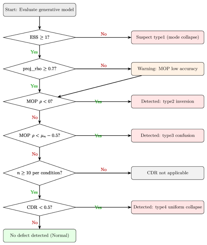
Appendix D.4. Worked Example: HPC-FNO-CFM Evaluation
This section illustrates the decision procedure by applying it to the HPC-FNO-CFM evaluation reported in Experiment 9 (Section 5-A). The model is a conditional Flow Matching model integrating a Fourier Neural Operator, evaluated on the NASA battery dataset across five temperature conditions (4, 8, 13, 24, 43 °C). Five variants are compared, differing in how many layers of the pre-trained FNO are retained during fine-tuning.
The worked example serves two purposes. It shows what each indicator detected in this evaluation. It also shows what each indicator could not detect, and what data conditions would be required for it to detect the corresponding defect. The second purpose is at least as important as the first for a practitioner deciding whether to apply this framework to a new dataset.
Appendix D.4.1. Pre-Evaluation: NASA Dataset
The NASA battery dataset provides –15 cells per temperature condition. For conditions with , CDR cannot produce reliable inter-condition distance estimates because the per-condition mean-vector distance is dominated by sampling noise at this sample size. In the controlled experiments of Experiment 14, a correctly conditioned CVAE generator yields CDR at , which would falsely indicate distance overestimation. As defined in the footnote accompanying Experiment 14, CDR is termed distance overestimation: the generated data place conditions further apart than the real data do. At per condition, the per-condition mean-vector estimates are dominated by individual cell variability, causing the estimated inter-condition distance to fluctuate far from its true value. The resulting CDR inflation is a consequence of the small sample size, not of any property of the generative model. CDR is therefore not applicable to the NASA battery dataset at its current sample size. To make CDR applicable, at least cells per condition are required. The current evaluation has 3–7 cells for most conditions.
The projection quality is , which exceeds the applicability threshold of 0.7. MOP is therefore applicable.
Appendix D.4.2. Layer 1 Diagnosis
With feature dimension and per-condition sample counts of 3–15, the Effective Stratum Size is for all conditions. All strata have ESS , indicating that the covariance matrices used in Fréchet distance computation are rank-deficient. SFD values for this dataset should therefore be treated as order-of-magnitude indicators rather than precise measurements. This is confirmed by the S-MMD comparison in Experiment 9. Despite a seven-order-of-magnitude range in SFD across the five variants, S-MMD values vary only between 0.22 and 0.31, indicating that the Fréchet distance differences reflect covariance estimation noise at least as much as the genuine quality differences.
The S-MMD values do distinguish the variants, though with much smaller separation than SFD. In the low-ESS regime, Layer-2 indicators that operate on mean vectors rather than covariance matrices provide more stable evidence.
Appendix D.4.3. Layer 2 Diagnosis
Table A15 reports the full three-layer diagnostic results for each variant, including the MOP value and diagnosis.
Table A15.
Three-layer diagnostic results for the five HPC-FNO-CFM variants on the NASA battery dataset (Experiments 9 and 10). SFD is the mean per-condition Fréchet distance (lower is better). CRC is the Spearman rank correlation of inter-condition distances (higher is better; range ). CDR is not reported because per condition on the NASA battery dataset. MOP is the Spearman rank correlation between projected per-condition centroids of the real and generated data (: ordering preserved; : ordering inverted). MOP diagnosis applies the thresholds established in Experiment 10.
The SFD values span seven orders of magnitude. freeze_2layer achieves the lowest mean per-condition Fréchet distance (2353), while pure_cfm reaches with catastrophic failure at 8 °C. This ordering reflects the degree of physical constraint imposed by the pre-trained FNO layers.
CRC reveals the structural integrity of each variant. freeze_2layer achieves the highest CRC (), indicating that the ordering of inter-condition distances is substantially preserved. pure_cfm achieves CRC , indicating that the physical structure across temperature conditions has been almost entirely destroyed, even if individual curves may appear plausible. freeze_3layer achieves CRC : the inter-condition distance ordering is essentially random, despite this variant achieving perfect temperature ordering (MOP ). This combination—correct ordering but scrambled distances—is itself a diagnostically meaningful finding. The variant preserves the direction of the temperature effect but not its magnitude structure.
MOP detects a type-2 inversion defect in freeze_2layer (MOP ). This means that freeze_2layer reproduces degradation curves in the wrong temperature order. The configuration with two frozen FNO layers appears to reverse the direction of the temperature extrapolation. freeze_3layer achieves MOP , confirming that freezing three layers preserves the temperature ordering correctly, even though the absolute curve quality is lower (SFD ).
The CRC result requires conditions for the NASA battery dataset, yielding condition pairs. The theoretical minimum p-value at is , so CRC can in principle achieve significance at this condition count. However, the empirical detection rate from Experiment 13 shows that is needed for reliable detection (80% rate) under random subsampling. With , the CRC results in Table A15 should be interpreted as directional evidence rather than statistically confirmed findings. To achieve reliable CRC detection on this dataset, additional temperature conditions would need to be included in the experimental design, bringing K to at least 8.
Appendix D.4.4. What the Evaluation Could Not Determine
CDR was not applicable because –7 cells per condition falls below the required . As a result, type-4 uniform collapse could not be formally assessed for any of the five variants. The CDR values observed in Experiment 9, which ranged from 4 to 958 across condition pairs, are inflated by sampling noise rather than reflecting genuine distance overestimation. To make CDR applicable to the NASA battery dataset, approximately 10 cells per temperature condition would be required, compared to the 3–7 currently available.
For the T/J confounding detection, the NASA battery dataset has a C-rate effect size of approximately 1.25, for which Experiment 8 indicates that approximately cells per condition are needed for the T/J ratio to achieve 80% detection. The current per-condition counts are near this threshold, so confounding detection is marginally feasible on the NASA battery dataset, unlike on the SNL battery dataset where the C-rate effect size of 0.426 would require approximately 50 cells per condition—roughly four times the available count.
Appendix D.4.5. Layer 3 Diagnosis
The near-uniform S-MMD values (0.22–0.31) across the five variants confirm low consistency between SFD and S-MMD for this dataset. The Layer-2 indicators (CRC, MOP) are therefore the primary diagnostic evidence for this evaluation.
Appendix D.4.6. Summary
Table A16 summarizes what each indicator detected, what it could not detect, and what data conditions would enable it.
Table A16.
Summary of diagnostic findings and data requirements for the HPC-FNO-CFM evaluation on the NASA battery dataset. The “requirement to enable” column states the data condition that would allow the indicator to produce reliable results on this dataset.
The most important diagnostic finding from this evaluation is the type-2 inversion in freeze_2layer. This model achieves the best per-condition generation quality (lowest SFD) and the best inter-condition distance ordering (highest CRC), yet it reproduces the temperature conditions in the wrong order (MOP ). This combination—high quality with inverted ordering—is a failure mode that neither FID nor CRC alone would reveal. FID cannot localize the inversion, and CRC measures distance ordering rather than temperature ordering. MOP is the only indicator in the framework that directly addresses this property, and this evaluation provides a concrete example of why it is necessary.
The evaluation also illustrates the data requirements for comprehensive diagnostics. With the current NASA battery dataset (5 conditions, 3–7 cells per condition), only SFD, CRC, and MOP can be applied. CDR and statistically confirmed CRC-based type-3 detection would require a redesigned experimental protocol with more cells per condition and more temperature conditions. These are conclusions about experimental design, not about the quality of the generative models under evaluation.
References
- Roman, D.; Saxena, S.; Robu, V.; Pecht, M.; Flynn, D. Machine learning pipeline for battery state-of-health estimation. Nat. Mach. Intell. 2021, 3, 447–456. [Google Scholar] [CrossRef] [Scilit]
- Plett, G.L. Battery Management Systems, Volume II: Equivalent-Circuit Methods; Artech House: Boston, MA, USA, 2015. [Google Scholar]
- Han, X.; Lu, L.; Zheng, Y.; Feng, X.; Li, Z.; Li, J.; Ouyang, M. A review on the key issues of the lithium ion battery degradation among the whole life cycle. eTransportation 2019, 1, 100005. [Google Scholar] [CrossRef] [Scilit]
- Severson, K.A.; Attia, P.M.; Jin, N.; Perkins, N.; Jiang, B.; Yang, Z.; Chen, M.H.; Aykol, M.; Herring, P.K.; Fraggedakis, D.; et al. Data-driven prediction of battery cycle life before capacity degradation. Nat. Energy 2019, 4, 383–391. [Google Scholar] [CrossRef] [Scilit]
- Dos Reis, G.; Strange, C.; Yadav, M.; Li, S. Lithium-ion battery data and where to find it. Energy AI 2021, 5, 100081. [Google Scholar] [CrossRef] [Scilit]
- Goodfellow, I.; Pouget-Abadie, J.; Mirza, M.; Xu, B.; Warde-Farley, D.; Ozair, S.; Courville, A.; Bengio, Y. Generative adversarial nets. In Proceedings of the Advances in Neural Information Processing Systems, Montreal, QC, Canada, 8–13 December 2014; Volume 27. [Google Scholar]
- Kingma, D.P.; Welling, M. Auto-encoding variational Bayes. arXiv 2014, arXiv:1312.6114. [Google Scholar]
- Ho, J.; Jain, A.; Abbeel, P. Denoising diffusion probabilistic models. In Proceedings of the Advances in Neural Information Processing Systems, Virtual, 6–12 December 2020; Volume 33, pp. 6840–6851. [Google Scholar]
- Lipman, Y.; Chen, R.T.Q.; Ben-Hamu, H.; Nickel, M.; Le, M. Flow matching for generative modeling. In Proceedings of the International Conference on Learning Representations, Kigali, Rwanda, 1–5 May 2023. [Google Scholar]
- Brophy, E.; Wang, Z.; She, Q.; Ward, T. Generative adversarial networks in time series: A systematic literature review. ACM Comput. Surv. 2023, 55, 1–31. [Google Scholar] [CrossRef] [Scilit]
- Yoon, J.; Jarrett, D.; van der Schaar, M. Time-series generative adversarial networks. In Proceedings of the Advances in Neural Information Processing Systems, Vancouver, BC, Canada, 8–14 December 2019; Volume 32. [Google Scholar]
- Desai, A.; Freeman, C.; Wang, Z.; Beaver, I. TimeVAE: A variational auto-encoder for multivariate time series generation. arXiv 2021, arXiv:2111.08095. [Google Scholar]
- Tashiro, Y.; Song, J.; Song, Y.; Ermon, S. CSDI: Conditional score-based diffusion models for probabilistic time series imputation. In Proceedings of the Advances in Neural Information Processing Systems, Virtual, 6–14 December 2021; Volume 34. [Google Scholar]
- Eivazi, H.; Hebenbrock, A.; Ginster, R.; Blömeke, S.; Wittek, S.; Herrmann, C.; Spengler, T.S.; Turek, T.; Rausch, A. DiffBatt: A diffusion model for battery degradation prediction and synthesis. arXiv 2024, arXiv:2410.23893. [Google Scholar] [CrossRef] [Scilit]
- Wu, B.; Widanage, W.D.; Yang, S.; Liu, X. Battery digital twins: Perspectives on the fusion of models, data and artificial intelligence for smart battery management systems. Energy AI 2020, 1, 100016. [Google Scholar] [CrossRef] [Scilit]
- Dubarry, M.; Howey, D.; Wu, B. Enabling battery digital twins at the industrial scale. Joule 2023, 7, 1134–1144. [Google Scholar] [CrossRef] [Scilit]
- Pang, G.; Shen, C.; Cao, L.; van den Hengel, A. Deep learning for anomaly detection: A review. ACM Comput. Surv. 2021, 54, 1–38. [Google Scholar] [CrossRef] [Scilit]
- Chen, C.; Zuo, Y.; Ye, W.; Li, X.; Deng, Z.; Ong, S.P. A critical review of machine learning of energy materials. Adv. Energy Mater. 2020, 10, 1903242. [Google Scholar] [CrossRef] [Scilit]
- Mayer, P.; Luzi, L.; Siahkoohi, A.; Johnson, D.H.; Baraniuk, R.G. Improving fairness and mitigating MADness in generative models. arXiv 2024, arXiv:2405.13977. [Google Scholar] [CrossRef] [Scilit]
- Heusel, M.; Ramsauer, H.; Unterthiner, T.; Nessler, B.; Hochreiter, S. GANs trained by a two time-scale update rule converge to a local Nash equilibrium. In Proceedings of the Advances in Neural Information Processing Systems, Long Beach, CA, USA, 4–9 December 2017; Volume 30. [Google Scholar]
- Stein, G.; Cresswell, J.C.; Hosseinzadeh, R.; Sui, Y.; Ross, B.L.; Villecroze, V.; Liu, Z.; Caterini, A.L.; Taylor, J.E.T.; Loaiza-Ganem, G. Exposing flaws of generative model evaluation metrics and their unfair treatment of diffusion models. Adv. Neural Inf. Process. Syst. 2023, 36, 3732–3784. [Google Scholar]
- Soloveitchik, M.; Diskin, T.; Morin, E.; Wiesel, A. Conditional Fréchet inception distance. arXiv 2021, arXiv:2103.11521. [Google Scholar]
- DeVries, T.; Romero, A.; Pineda, L.; Taylor, G.W.; Drozdzal, M. On the evaluation of conditional GANs. arXiv 2019, arXiv:1907.08175. [Google Scholar]
- Attia, P.M.; Grover, A.; Jin, N.; Severson, K.A.; Markov, T.M.; Liao, Y.H.; Chen, M.H.; Cheong, B.; Perkins, N.; Yang, Z.; et al. Closed-loop optimization of fast-charging protocols for batteries with machine learning. Nature 2020, 578, 397–402. [Google Scholar] [CrossRef] [Scilit] [PubMed]
- Saha, B.; Goebel, K. Battery data set. In NASA Prognostics Data Repository; NASA Ames Research Center: Moffett Field, CA, USA, 2007. [Google Scholar]
- Tan, R.; Hong, W.; Tang, J.; Lu, X.; Ma, R.; Zheng, X.; Li, J.; Huang, J.; Zhang, T.Y. BatteryLife: A comprehensive dataset and benchmark for battery life prediction. In Proceedings of the 31st ACM SIGKDD Conference on Knowledge Discovery and Data Mining V.2, Toronto ON, Canada, 3–7 August 2025; KDD ’25, pp. 5789–5800. [Google Scholar] [CrossRef] [Scilit]
- Okita, T. Excluding the Target Domain Improves Extrapolation: Deconfounded Hierarchical Physics Constraints. arXiv 2026, arXiv:2605.07485. [Google Scholar] [CrossRef] [Scilit]
- Benny, Y.; Galanti, T.; Benaim, S.; Wolf, L. Evaluation Metrics for Conditional Image Generation. Int. J. Comput. Vis. 2021, 129, 1712–1731. [Google Scholar] [CrossRef] [Scilit]
- Mirza, M.; Osindero, S. Conditional generative adversarial nets. arXiv 2014, arXiv:1411.1784. [Google Scholar] [CrossRef] [Scilit]
- Sohn, K.; Lee, H.; Yan, X. Learning structured output representation using deep conditional generative models. In Proceedings of the Advances in Neural Information Processing Systems, Montreal, QC, Canada, 7–12 December 2015; Volume 28. [Google Scholar]
- Ho, J.; Salimans, T. Classifier-free diffusion guidance. arXiv 2022, arXiv:2207.12598. [Google Scholar] [CrossRef] [Scilit]
- Fawaz, H.I.; Lucas, B.; Forestier, G.; Pelletier, C.; Schmidt, D.F.; Weber, J.; Webb, G.I.; Idoumghar, L.; Muller, P.A.; Petitjean, F. InceptionTime: Finding AlexNet for time series classification. Data Min. Knowl. Discov. 2020, 34, 1936–1962. [Google Scholar] [CrossRef] [Scilit]
- Koochali, A.; Walch, M.; Thota, S.; Schichtel, P.; Dengel, A.; Ahmed, S. Quantifying quality of class-conditional generative models in time series domain. Appl. Intell. 2023, 53, 24530–24550. [Google Scholar] [CrossRef] [Scilit]
- Kansal, R.; Li, A.; Duarte, J.; Chernyavskaya, N.; Pierini, M.; Orzari, B.; Tomei, T. Evaluating generative models in high energy physics. Phys. Rev. D 2023, 107, 076017. [Google Scholar] [CrossRef] [Scilit]
- Good, P.I. Permutation Tests: A Practical Guide to Resampling Methods for Testing Hypotheses, 2nd ed.; Springer: Berlin/Heidelberg, Germany, 2000. [Google Scholar]
- Spearman, C. The Proof and Measurement of Association between Two Things. Am. J. Psychol. 1904, 15, 72–101. [Google Scholar] [CrossRef] [Scilit]
- Efron, B.; Tibshirani, R.J. An Introduction to the Bootstrap; Chapman & Hall: London, UK, 1994. [Google Scholar]
- Mann, H.B.; Whitney, D.R. On a Test of Whether One of Two Random Variables is Stochastically Larger than the Other. Ann. Math. Stat. 1947, 18, 50–60. [Google Scholar] [CrossRef] [Scilit]
- Gretton, A.; Borgwardt, K.M.; Rasch, M.J.; Schölkopf, B.; Smola, A. A kernel two-sample test. J. Mach. Learn. Res. 2012, 13, 723–773. [Google Scholar]
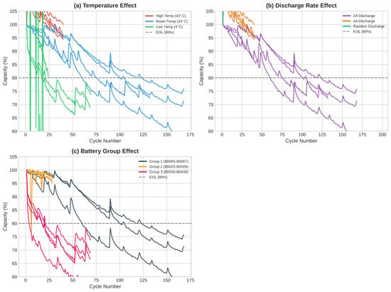
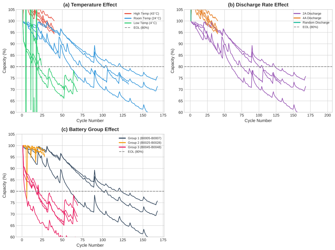
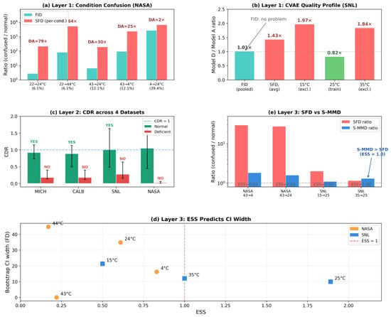
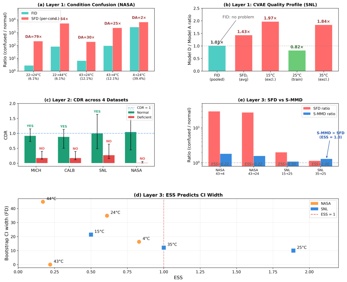
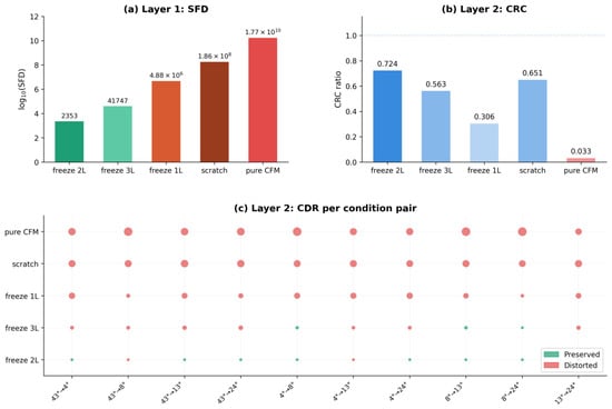
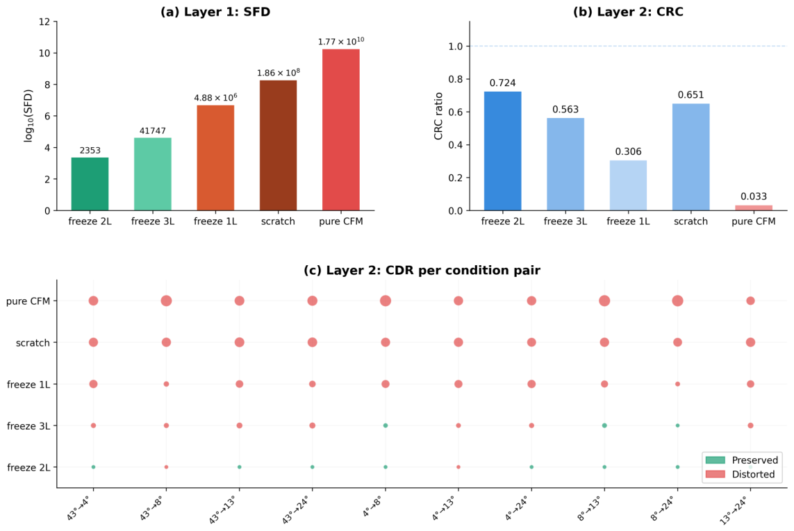
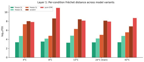
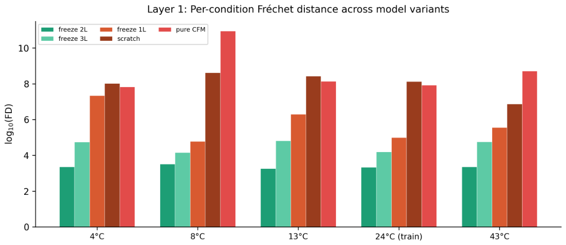

Disclaimer/Publisher’s Note: The statements, opinions and data contained in all publications are solely those of the individual author(s) and contributor(s) and not of MDPI and/or the editor(s). MDPI and/or the editor(s) disclaim responsibility for any injury to people or property resulting from any ideas, methods, instructions or products referred to in the content. |
© 2026 by the author. Licensee MDPI, Basel, Switzerland. This article is an open access article distributed under the terms and conditions of the Creative Commons Attribution (CC BY) license.