Abstract
Quantifying livelihood vulnerability to wildland fires in the United States is challenging because of the need to systematically integrate multidimensional variables into its analysis. We aim to measure wildfire threats amongst humans and their physical and social environment by developing a framework to calculate the livelihood vulnerability index (LVI) for the top 14 American states most recently exposed to wildfires. The LVI is computed by assessing each state’s contributing factors (exposure, sensitivity, and adaptive capacity) to wildfire events. These contributing factors are determined through a set of indicator variables that are categorized into corresponding groups to produce an LVI framework. The framework is validated by performing a principal component analysis (PCA), ensuring that each selected indicator variable corresponds to the correct contributing factor. Our results indicate that Arizona and New Mexico experience the greatest livelihood vulnerability. In contrast, California, Florida, and Texas experience the least livelihood vulnerability. While California has one of the highest exposures and sensitivity to wildfires, results indicate that it has a relatively high adaptive capacity, in comparison to the other states, suggesting it has measures in place to withstand these vulnerabilities. These results are critical to wildfire managers, government, policymakers, and research scientists for identifying and providing better resiliency and adaptation measures to support states that are most vulnerable to wildfires.
1. Introduction
Wildfires are crucial for ecosystem dynamics by balancing fuel types and creating appropriate vegetation for maintaining healthy forested regimes [1]. Despite the integral ecological role of wildfires, uncontrolled burns can cause widespread environmental, economic, social and sustainable development impacts [2,3,4]. Such wildfire impacts include losses to human lives; incurring financial losses from buildings and homes; widespread social, health and economic costs through evacuations, smoke exposure, and loss of tourism revenue [5,6,7]. The Insurance Information Institute, gives an example of financial loss due to wildfires, including the 2019 wildfires in California and Alaska that created a loss of 4.5 billion dollars in damages, largely resulting from the California Kincade and Saddle Ridge wildfires. In order to minimize ignition and spread during this time, California’s electrical utility provider issued rolling blackouts to homes and businesses during high wind and extreme dry conditions. However, this inevitably cost the state billions of dollars in losses [8]. It is therefore evident that wildfires have a direct impact on the livelihood of many residents in fire-prone communities within the United States, making them vulnerable to wildland fire exposure [9].
Besides economic impacts, changes in social and climate conditions can significantly affect fire regimes, producing greater potential damage than those previously thought [2]. Social factors, such as the expansion of the wildland–urban interface (WUI) (where human settlements, buildings, and wildland vegetation meet), have influenced the dramatic increase in wildfire suppression costs, as well as the number of homes lost to wildfires in the United States (US) over the past 30 years [7,10,11]. The 2019 wildfire risk report shows that the US experienced the sixth-highest acres burned in 2018 since the mid-1900s. According to the National Interagency Fire Center (NIFC) report, California has topped the list in the US with over 1.8 million acres burned in 2018 [12]. Climate factors such as extreme weather conditions can also influence the escape of wildland fires during suppression practices, leading to unplanned destructive fire behavior [7,13], thereby worsening environmental and socio-economic impacts.
There have been many wildfire risk assessment studies that use a wide range of wildfire danger indices [14]. However, many of these indices focus mainly on specific hazard components of wildfires (behavior, danger, threat) and consider biophysical components of weather conditions, topography, fuel, fire size, rate of spread, suppression difficulty, fire occurrence, or burn severity to generate fire risk assessment maps [15]. Studies, such as that of [16], have evaluated fire risk on structures, taking into account variables pertaining to topography, spatial arrangement, and vegetation. However, meteorological factors (atmosphere and weather patterns), building materials, and fire suppression efforts within different fire regions are also important to consider. It is acknowledged that combining these various multidimensional socio-economic and biophysical variables into a risk and vulnerability assessment framework can be challenging. While various studies have attempted to bridge the gaps among the social, natural, and physical sciences and contributed to new methodologies that confront this challenge [17,18,19,20], not much of this approach has been applied to specifically assess wildfire vulnerability in wildland fire prone regions of the US. Therefore, there is a need to systematically integrate multidimensional variables into a framework to evaluate wildfire vulnerability in highly exposed wildland fire regimes, a method often lacking in other risk assessment studies. Thus, the integration across scales and disciplines to produce a wildfire vulnerability assessment can be conducted by creating a framework to assess the livelihood vulnerability of highly exposed regions to wildfires. A livelihood vulnerability framework incorporates not only wildfire exposure in a particular region (such as biophysical factors), but also quantifies the sensitivity of a region to wildfire exposure, and its ability to withstand these biophysical exposures (known as adaptive capacity). Thus, producing a livelihood vulnerability framework is an appropriate method for assessing the vulnerability of communities to wildfire exposure because it not only takes into account biophysical factors, but also considers socio-economic influences.
A common thread in the literature is the attempt to quantify multidimensional parameters (biophysical, social, and economic) using diverse indicator variables as proxies that can be integrated and combined to produce a vulnerability assessment, as in the work of [21] who investigated a sustainability livelihood approach [18]. The field of climate vulnerability assessment, as a whole, has evolved to address the need to quantify the ability of communities to adapt to changing environmental conditions [18] (such as changes in wildfire exposure). Thus, a vulnerability assessment is appropriate for describing a diverse set of methods that are used to systematically integrate and examine interactions between humans and their physical and social environment [18].
The definition of the term vulnerability, exposure, sensitivity, and hazards vary among disciplines [22,23]. However, there is similar consensus in the definition of vulnerability to climate change by the IPCC and Food and Agriculture Organization (FAO). These studies define vulnerability as the extent or degree to which a system (geophysical, biological, or societal) is at risk and incapable of thriving under negative effects of an exposure (such as climate change) [23,24]. The livelihood vulnerability addresses how a system’s basic necessities of living, such as shelter, work conditions, health and environment are affected by an exposure, such as wildfires. Studies, such as that by [18] have combined previous climate vulnerability methods to construct a livelihood vulnerability index (LVI) to estimate the differential impacts of climate change on several African communities. Their method follows heavily on the working definition of vulnerability as a function of three contributing factors (exposure, sensitivity and adaptive capacity) as defined by the Intergovernmental Panel on Climate Change (IPCC) (IPCC, 2001). Exposure represents the magnitude and duration of the climate-related exposure (in our case wildfires), while sensitivity describes the degree to which a system is affected by the exposure, and adaptive capacity describes the system’s ability to withstand or recover from the exposure [17,25].
The LVI uses multiple indicators that are aggregated into the IPCC’s three contributing factors to produce a vulnerability framework. Studies have applied the LVI method, such as [26] to assess farmers’ livelihood vulnerability to global changes in irrigation agricultural practices in Spain. They show that an increase in the adoption of irrigation practices have increased the short-term adaptive capacity while displacing small-scale farming. Studies, such as [27], have also used the LVI approach to assess the livelihood vulnerability of flood risks to farmers for different regions in Indonesia. Results indicate that regions with similar physical characteristics and agricultural dependencies show similar vulnerability levels. A study [28] used LVI to quantify the vulnerability of communities to heavy lake effect snowfall in the Northwest Territories of Canada. They found that extreme precipitation makes some lake-rich communities more vulnerable than communities farther inland. Therefore, it is acknowledged that there are numerous interpretations on how best to apply exposure, sensitivity, and adaptive capacity concepts to quantify vulnerability [17,25,29,30,31,32], with key differences among studies that include methods used for scaling, gathering, grouping, and aggregating indicator variables [18].
We adopt an LVI approach, similar to the original methods proposed by [18], to evaluate recent wildfire impacts in the US. This is conducted by developing a framework that combines a set of indicator variables into their respective contributing factors to determine the critical biophysical and human dimension components influencing the livelihood vulnerability of selected wildfire prone states. The information gained from this assessment will provide a clearer understanding as to which states are most vulnerable to wildfires despite their level of wildland fire exposure. This information will be critical to researchers, government organizations, and policymakers for identifying, allotting, and providing better resiliency and adaptation measures, such as aiding in financial, environmental, and social support for states that are most vulnerable to wildfires.
2. Data and Methodology
Assessing the LVI to wildfires across selected American states are conducted in two folds. First, we develop a framework comprising a set of biophysical, social, and economic factors that is used to assess each state’s livelihood vulnerability to wildfires. We acknowledge that our framework provides one possible way of developing a livelihood vulnerability model, and that results could differ depending on the subjective allocation of each indicator variable in our framework. For these reasons, we also conduct a principal component (PCA) analysis to determine the validity of our framework. Second, we calculate the LVI and its contributing factors for each state. We further conduct a sensitivity test to provide additional certainty that our framework is valid, and our results are robust.
2.1. Building the LVI Framework
The definitions of the livelihood vulnerability terms used in our framework are summarized in Table A1, which describes the overarching contributing factors comprising exposure, sensitivity, and adaptive capacity (color coded red, blue, and green, respectively). While we acknowledge that the definition of the vulnerability terminologies can differ across disciplines, we develop our framework and conduct our livelihood vulnerability assessment based on the definitions in Table A1, to ensure terminology and interpretation consistency throughout this study. These contributing factors are divided into major components (first level of divisions within each contributing factor). These major components are further divided into sub-components (second level of divisions within each major component) and subsequent indicator variables (measurable units of data for each sub-component) (Figure 1).
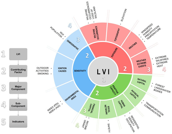
Figure 1.
Description of the framework developed for the LVI (box 1 and the central gray circle). LVI is represented by contributing factor (box 2). The contributing factors are sensitivity (blue), exposure (red), and adaptive capacity (green). The contributing factors are further divided into major components (box 3). The major components are color-coordinated with the contributing factors. The major components for sensitivity (blue) are demographic, ignition causes, and environmental index (light blue); for exposure (red) are wildfire occurrence, topography, weather, weather extreme events (light red); for adaptive capacity (green) are social network, natural, physical, human, and financial capital (light green). Major components are divided into sub-components (box 4) and represented by the sub-components in the outermost part of the circle. The sub-components are further divided into indicators (box 5) and not shown in this figure. Refer to Table A2 for each indicator variable.
In our study, the exposure factor pertains to wildfire danger and the physical processes that influence the intensity and severity of fire behavior. Major components within exposure are wildfire occurrence, topography, weather, and extreme weather events. In our framework, an indicator variable under exposure is interpreted as variables that can adversely affect the exposure of wildfire risk to people within a state. For example, “total acres burnt due to wildfires” is an indicator variable that represents how burnt soil disturbs hydrologic and soil conditions leading to increased likelihood of flooding, runoff, and debris flow [33]. This variable can be interpreted as, the greater the number of acres burnt, the greater the exposure humans have to “knock-on” natural hazards, such as flash flooding and landslides within a state (Table A2).
Sensitivity describes the degree to which each state is affected by wildfires. Its major components are demographic, ignition causes, and selected environmental indices. The indicator variables under sensitivity are interpreted as variables that contribute to a state’s sensitivity to wildfires. For example, the “number of houses within a wildland urban interface zone” is an indicator variable under sensitivity because WUI are high-risk wildfire regions due to their accumulation of wildland vegetation, concentration of flammable human structures, and potential ignition sources from sparks left by human activities [34,35]. Therefore, this indicator is interpreted as follows: States with larger WUI area and greater number of homes within the WUI will be at increased risk and sensitivity to wildfires (Table A2).
Adaptive capacity describes the ability of each state to withstand or recover from wildfires. The major components of adaptive capacity include natural capital, physical capital, human capital, social network, and financial capital. The indicator variables under adaptive capacity are interpreted as variables that can positively contribute to the state’s mitigation and adaptive strategies for wildfires. For example, “median household income” is an indicator variable under adaptive capacity that can be interpreted as: States with higher income may have more financial resources and financial capital to invest in home and community hardening, thereby having higher mitigation and adaptation capacities (Table A2).
When interpreting the indicator variables under each contributing factor (exposure, sensitivity, and adaptive capacity), usually states with higher values would represent greater exposure, sensitivity, or adaptive capacity to wildfires. For example, states with higher temperatures would have a “greater exposure to wildfires”. However, for certain indicator variables, the opposite is true, such as precipitation. States with higher amounts of precipitation will have a “lower” exposure to wildfires. Indicator variables that are interpreted as such require the inverse of their value to be integrated into the LVI equation (e.g., instead of 12 mm of rain, it would be (). These inverse indicators are denoted with an asterisk (*) in Table A2. Please refer to Table A2 for a comprehensive overview of our LVI framework that outlines all the major components, sub-components, and indicator variables used in each contributing factor, along with detailed rationales and interpretation on how we apply each indicator variable to assess the livelihood vulnerability of each state.
2.2. Input Variables
The LVI analysis is conducted solely for 14 fire prone American states that are most at risk to wildfires. The states selected are Arizona, California, Florida, Idaho, Montana, Nevada, New Mexico, Oklahoma, Oregon, Utah, Washington, and Wyoming because they experienced the highest risk of wildfires in 2018, as determined from by the maximum acres burnt in 2018 and 2019 and as documented in the NIFC 2019 Wildfire Risk Report (Table A3 in the Appendix A). The 14 states analyzed in this study had the largest acreage burnt in 2018 across the US (Figure 2). For these reasons, we limit our analysis to comparing the LVI for only the top states most exposed to wildfires. The remainder of the states are not as exposed and will inevitably provide irrelevant comparisons. Though Alaska was included as a top state listed in the 2019 Wildfire Risk Report, it was excluded from our study due to the lack of spatial and temporal comprehensive data, such as those required under sensitivity (e.g., number of houses within the WUI zone), and if included, would have impeded our comparison analysis among the other states.
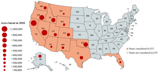
Figure 2.
Map of the United States with the states that are analyzed shaded in orange and states not considered shaded in gray. The acreage size burnt in 2018 and 2019 is indicated by the red circles, ranging from the smallest circle (burn area less than 90,000 acres) to the largest circle (burn area exceeding 1 million acres).
Our analysis is conducted to determine the current LVI and not future LVI projections. Therefore, most of the data gathered for our assessment were acquired within the past decade (2010–2019). The exception is given to certain indicator variables that represent a long-term climatological average (1950 to 2019). In addition, the elevation data for each state was acquired from 1980, with the understanding that the elevation of each state is not time sensitive and would not have changed drastically if the measurements were acquired in 2019. The year in which the data was acquired for each indicator variable in our framework is indicated in Table A2.
Furthermore, most of the data acquired are entered directly into the framework as raw values, meaning that they did not require additional computations before the LVI was calculated. However, some indicator variables under exposure, sensitivity, and adaptive capacity required further processing to be amenable and included in the analysis. Indicator variables under the exposure that required initial computations included annual average wind speed, humidity, annual precipitation, number of days with higher than 0.1 inches or more of precipitation, and annual temperature. The National Center for Environmental Information (NCEI) provides annual averages of each indicator for various weather observation stations located in each state. The values for every available weather observation station within each state were spatially averaged over the state and temporally averaged over the 1950 to 2018 period before being used in our LVI calculations.
The indicator variables requiring initial computation under sensitivity included the Palmer Drought Index (PDI) and the number of smokers. The National Oceanic and Atmospheric Administration (NOAA) collects monthly PDI values from weather observation stations throughout the US every year. The 2019 annual average was calculated for each station and then averaged amongst all the stations within a state. We also calculated the number of smokers using data from the United Health Foundation, which provided the percentages of smokers for every state. To accurately convey the proportions between the states, the state’s population for that year was multiplied by its respective percentage of smokers. Finally, for adaptive capacity, only the indicator variable pertaining to the total area of lakes had to be computed. The original data provided the area for each individual lake. Thus, we had to aggregate the area for all lakes to produce the cumulative lake area in each state.
The motivation for including the selected indicator variables in our framework was based on current risk assessment information suggested by the open literature, such as potential health risks due to wildfires [36]. Other examples include indicator variables pertaining to fuel, weather, and topography that are important drivers of wildfire danger and behavior, as referenced heavily in the literature [37,38]. Environmental indices such as the PDI and air quality were also included. While we acknowledge that there are many fire indices that could be integrated [14], we selected PDI because of its available spatial and temporal data for our study and because PDI is a useful indicator in describing an essential environmental factor (drought) required for the potential onset, ignition, and behavior of a wildfire [39]. Adding more fire indices and sub-indices would add redundancy to our framework.
2.3. LVI Calculation
Subsequently, we calculate the LVI and the corresponding contributing factors for each of the analyzed states based on our developed framework (Table A2). Our methods for computing the LVI follows a similar approach to [18,27]. Before the computation, we need to interpret whether the magnitude of each indicator value, under each contributing factor, is influencing the contributing factor positively or negatively. If the indicator variable is affecting the contributing factor negatively, then the inverse value is taken.
To compute LVI, we first compute the standardized index () for each indicator variable, where , is the original indicator variable for each individual state, and represent the state with the maximum and minimum value, respectively, corresponding to that particular indicator, we use Equation (1).
Second, the major component () value for each state is computed by averaging the standard indices, over the number () of all indicators used in each major component, as in Equation (2).
Third, each contributing factor is computed by taking a weighted average of each computed major component. This is done by multiplying each major component by its number of indicators (), as in Equation (3).
Finally, the LVI for each state is computed by combining the contributing factors of exposure , adaptive capacity , and sensitivity , as in Equation (4).
The weighted balance function is applied to this method, as followed by [18]. The weighted function gives equal weighting to each indicator variable, despite how many indicators are present within the framework. This weighted approach is often used when determining vulnerability in data-scare regions. Once the LVI is computed for each state, a constant value of 0.5 is added to each LVI to simply aid in visualizing and interpreting the rank of LVI [26].
2.4. Validation Framework Approach
We subsequently applied a PCA to our indicator variables in order to gain confidence in the structure of our framework. PCA is a variable-reduction technique that takes a large set of variables and organizes them into a smaller set of principal components. For the purposes of this study, PCA was used to verify our framework by ensuring the indicator variables were loading into the “proper” major components that they were assigned. When conducting a PCA, four assumptions are made about the dataset, namely (1) the variables are measured at the continuous level, (2) there is a linear relationship between the variables, (3) there is adequate sample size, and (4) the dataset contains no outliers [40]. In addition, two tests are conducted to determine whether PCA is a suitable method for validating our framework: the Kaiser–Meyer–Olkin (KMO) sampling adequacy test [41] and Bartlett’s Test of sphericity [42]. The KMO test measures the proportion of variance among the indicator variables that may be caused by underlying factors. KMO is an average of the measure of sample adequacy (MSA) for each indicator variable within their respective major component. MSA values range from 0 to 1 and represent the extent of a given indicator belonging to a group [43]. Smaller KMO values indicate fewer correlations between a given variable and the other indicators. Therefore, if the KMO value is less than 0.5, the results from a PCA will not be useful because the indicators do not share high correlations with each other. From Table A4 in the Appendix A, KMO values range mostly between 0.5 and 0.8, suggesting a strong sampling adequacy. Bartlett’s test of sphericity is conducted to determine whether the correlation matrix of the indicators is an identity matrix. The null hypothesis is that the indicators are orthogonal (uncorrelated). For this study, if the indicator variables are uncorrelated, then they are unsuitable for this factor analysis. The values for this test range from 0 to 1, with 0 representing a rejection of the null hypothesis (meaning that the indicator variables are correlated). In addition, a significance value that is less than 0.05 indicates that PCA will provide helpful information. The values for the Bartlett’s test of sphericity in our results mostly range from 0 to 0.3, suggesting that the variables chosen are correlated. Table A4 in the Appendix A provides the KMO and Bartlett test scores for each major component by using the indicator data gathered from the 14 states.
Once the indicator variables we selected had passed these tests, a PCA was conducted. The normalized data input for PCA were the standardized values for each indicator. The PCA gives insightful data such as a correlation matrix, communalities, and total variance explained. However, the output that helped reorganize and strengthen our framework was the component matrix. The component matrix displays the Pearson correlations between the indicator variables and principal components. The component matrix was used to verify whether the indicator variables loaded into their respective major components. This indicates that they are measuring the same underlying construct and are, therefore, correctly grouped accordingly in our framework.
Apart from the added confidence we gain from applying the PCA, we also conduct a sensitivity analysis to test whether our framework provides robust livelihood vulnerability results for each state. This is conducted by slightly perturbing our framework (through randomly selecting to omit one indicator variable at a time from a major component) and then re-running the LVI calculations. This will, thereby, provide twelve different framework scenarios with LVI results generated for each state. The original LVI results (current framework) is compared to the LVI output from each scenario to establish whether the top three LVI states and the lowest three LVI states remain consistent throughout 90% of the runs. If the LVI ranks remain the same (or are similar within reason) for more than 90% of the runs, these results provide additional validation to the framework. Refer to Table A8 for a synthesis of the scenarios. We acknowledge that other scenarios may be possible (by interchanging some indicator variables amongst the contributing factors) but this would lead to many other possible scenarios and has already been tested by the PCA.
3. Results
3.1. LVI
We compute the LVI for each of the 14 American states analyzed (Figure 3). Most of the states we analyzed exhibit similar LVI values. However, Arizona and New Mexico experience the greatest livelihood vulnerability, with an LVI of 0.57 and 0.55, respectively. In contrast, California, Florida, and Texas experience the least livelihood vulnerability to wildfires (0.44, 0.35, 0.33, respectively) (Figure 4). To understand these LVI results, we delve into analyzing each contributing factor.
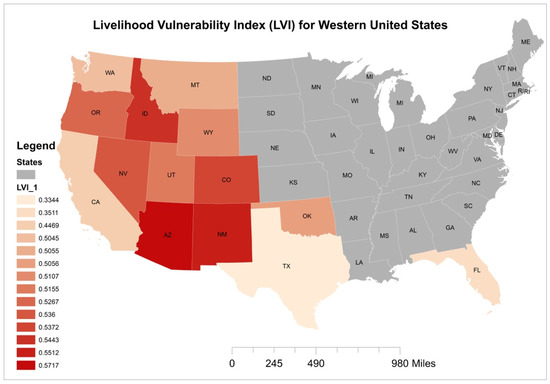
Figure 3.
Map of each states’ LVI value, with its magnitude corresponding to the color bar where darker red indicates the highest LVI. States shaded gray have not been analyzed in this study.
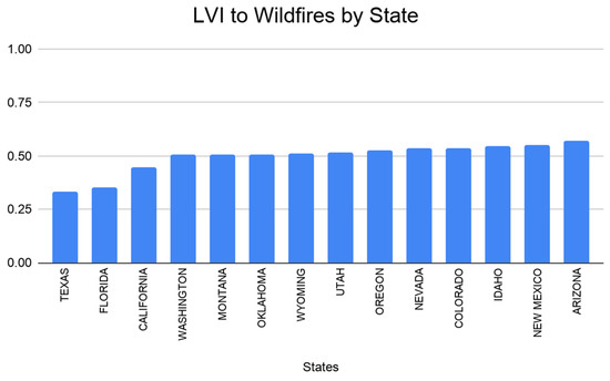
Figure 4.
Histogram showing the LVI of the 14 selected states in the US with Arizona having the highest LVI and Texas having the lowest LVI.
3.2. Exposure
First, we examine each state’s susceptibility to wildfire by examining the exposure contributing factor. The exposure results indicate that California, Nevada, and Arizona exhibit the highest exposure to wildfires (0.63, 0.52 and 0.49, respectively) while Oklahoma, Florida, and Montana have the least exposure (0.25, 0.21 and 0.19, respectively) (Figure 5a). To understand the exposure results, we assess the four major components of exposure (wildfire, topography, weather, and weather extreme events) for each state Figure 5b). Wildfires (blue) is predominant for California, Texas, and Arizona. This is because these states experience the highest number of wildfires and the largest acres burnt due to wildfires in 2019. Nevada and Arizona also experience relatively higher values of weather (yellow), which indicate favorable weather conditions for the development of wildfires, such as relatively higher wind speeds and lower humidity. In addition, weather extreme events (green) represent extreme wildfire and extreme heat events and are most prevalent in California and Nevada.
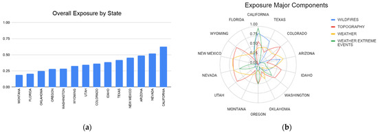
Figure 5.
Histogram showing the overall exposure of the 14 selected states in the US with California having the highest exposure (with respect to wildland fire) and Texas having the lowest overall exposure (a). Radar plot showing the different major components of the exposure contributing factor, namely, wildfires (blue), topography (red), weather (yellow), and weather extreme events (green) for the selected 14 states of the US (b).
The major component, topography, represents mean height and highest elevation for each state. Topography is important because higher elevations in complex terrain can be conducive to the propagation of wildfire behavior, add uncertainties to the prediction of the wildfire rate of spread [44], and make fire suppression efforts more challenging. Thus, states with higher topographic values could potentially be more at risk, or dangerously affected by wildfires. Nevada also ranks high in topography. While topography is also relatively high for other states, such as Wyoming and Utah, other major components, such as wildfires, weather, and weather extremes, are negligible, thereby reducing the overall exposure of wildfires in these states. Furthermore, Florida, Oklahoma, and Montana have the lowest exposures because all of their major components under exposure are ranked very low in comparison to the other states.
3.3. Sensitivity
Second, we assess the degree to which each state is affected by wildfires by investigating the sensitivity contributing factor. The results for sensitivity (Figure 6a) show California as the most sensitive state to wildfires (0.84). This is followed by Texas, with a sensitivity of 0.66. Montana and Wyoming are the least sensitive. California, Texas, and Florida are the most sensitive to wildfires because they yield the highest values of each major component under sensitivity (demographic, ignition causes, and environmental index) (Figure 6b). Demographic comprises sub-components, such as the wildland-urban interface (WUI) and population. States with larger WUI areas or higher populations within a WUI, would be more sensitive to wildfires because they are within a region more exposed to wildfire events. Ignition causes attributed to outdoor activities, such as campfires and smoking, would also increase the potential inception of human-caused fires. In addition, states that experience poorer air quality and more drought will be more sensitive during and after wildfire events and seasons. The environmental index remains relatively constant among all states (yellow). However, California and Texas are the most sensitive states because they are driven primarily by the major components of ignition causes (red) and demographic (blue). The least sensitive state is Montana (0.08) because, in comparison to the other states, all its major components are ranked relatively low.
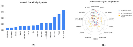
Figure 6.
Histogram showing the overall sensitivity of the 14 selected states in the US with California having the highest sensitivity (with respect to wildland fire) and Texas having the lowest overall sensitivity (a). Radar plot showing the different major components of the sensitivity contributing factor, namely, demographic (blue), ignition causes (red), and the environmental index (yellow) for the selected 14 states of the US used in this study (b).
3.4. Adaptive Capacity
Third, we assess the ability of each state to withstand or recover from wildfires by analyzing the contributing factor of adaptive capacity. Our results indicate that California, Texas, and Florida exhibit the greatest adaptive capacity to wildfires (0.69, 0.67 and 0.48, respectively) while Oregon, Idaho, and Montana are the least adaptive (0.15, 0.12, 0.12, respectively) (Figure 7a). The reasons for the adaptive capacity disparities among the states have to do with the major components (or capitals) that each state has (natural, physical, human, social network, and financial) Table A2.
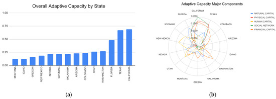
Figure 7.
Histogram showing the overall adaptive capacity of the 14 selected states in the US with California having the highest adaptive capacity (with respect to wildland fire) and Texas having the lowest overall adaptive capacity (a). Radar plot showing the different major components of the adaptive capacity contributing factor, namely, natural capital (blue), physical capital (red), human capital (yellow), social network (green), and the financial capital (orange) for the selected 14 states of the US (b).
What drives the adaptive capacity to be relatively high for California and, to a slightly lesser extent, Texas, are their social network (green) physical capital (red) and financial capital (orange) (Figure 7b). These two states have social structures in place to facilitate safety measures in times of wildfires such as allocating firefighters and first responders to wildland fire emergencies. These states are also more equipped with transportation accessibilities, such as closer airports and access to public roads, in case of major wildfires. California and Texas also have greater access to communication within their households, including internet signals for receiving warning alerts, both of which can be beneficial to one’s livelihood during the state of an emergency wildfire evacuation. These states also rank highly in financial capital, such as having relatively higher household incomes and fire management assisted grants, which can lend financial support during wildland fire emergency hazards. Additionally, Florida also has a high adaptive capacity that is primarily driven by its natural capital. It has the largest water area of all the states analyzed, thereby providing the state with water resources for fire suppression.
In contrast to the states with the highest adaptive capacity, Montana, Idaho, and Oregon rank very low in all capitals. Moreover, while some states rank high in one major component, it suffers in others, thereby driving down the rank of its overall adaptive capacity value. For example, New Mexico has a relatively high human capital in comparison to other states, which corresponds to residential density and occupation; however, all its other capitals are negligible, resulting in an overall low adaptive capacity to wildfires. This emphasizes the need to evaluate all the contributing factors in adaptive capacity to obtain a holistic view of the allotted resources available to aid in wildfire resiliency measures. Adaptive capacity is one of the most important determining factors in risk assessment, as highlighted by [45]. who showed that wildfire hazard potential can be reduced once the adaptive capacity of the state is taken into consideration.
4. Discussion
4.1. Validation of Framework
4.1.1. Principal Component Analysis (PCA)
A PCA was conducted for each major component to test the indicators categorized within them. Table A4 in the Appendix A shows the results after running the KMO and Bartlett test. All of the values from the KMO test are at least 0.5, which is the minimum required value to conduct a PCA as described in [41]. The only major component that is not at least 0.5 is that of weather, which has a value of 0.488. Previous research such as [46] suggests a KMO value of at least 0.6 in order to proceed with PCA. However, due to the small sample size and indicators tested per PCA (adaptive capacity, 13; exposure, 11; sensitivity, 9) it is difficult to achieve a KMO value of at least 0.6. In addition, in this study, PCA was not utilized for its typical purpose of reducing variables, but rather, performed to verify whether the indicators within each major component loaded onto one principal component.
Table A4 in the Appendix A also contains the results for the Bartlett test. Some of the major components achieved a desirable value of less than 0.05. However, some had values higher than 0.05. This is not an issue for two reasons. First, the major components that had a value greater than 0.05 had only two indicators to test. Only having two variables to create a correlation matrix would make it very difficult to achieve a value below 0.05. Second, the purpose of conducting a Bartlett test is to assess whether the correlation matrix diverges significantly from an identity matrix for data reduction [47]. Since the goal of the PCA is not variable reduction, the correlation matrix only needed to be proven as not being an identity matrix, that is, a value closer to 0 than 1.
After computing the PCA, we analyzed the generated component matrices. To validate the framework, the indicators had to have a strong loading into their respective major components. A strong loading is considered to be any value above 0.5 and suggests that the indicators are measuring the same underlying construct. Despite the fact that a PCA was conducted for each major component, the results are compiled into three tables (Table A5, Table A6 and Table A7 in the Appendix A), one for each contributing factor. Overall, most of the indicators demonstrated a strong loading into their respective major components. However, there were some indicators that had weak loadings, under a value of 0.5, for example, annual average wind speed and annual average temperature in exposure. These indicators had a factor loading of 0.17 and 0.39, respectively, for the major component of weather. These low values indicate an inverse relationship between the other indicators under weather [48]. When a state is characterized by higher wind speed and temperature, they are more likely to be exposed to wildfires. The other indicators under weather involve humidity and precipitation. If a state is characterized by higher humidity and precipitation, then they are less likely to be exposed to wildfires in that same year. The same logic can be applied to the following indicators: acres of forests, number of timber/woodworkers, and annual PDI. These indicators all have negative loadings for their respective major components. These inverse relationships were reflected in the calculation of the LVI. With PCA verifying the structure of our framework, the validity of the LVI results is strengthened.
4.1.2. Sensitivity Analysis
Another test to validate our framework, included a sensitivity analysis. We perturbed the framework by removing one indicator variable at time and testing the rank of the new LVI results. A total of twelve scenarios were conducted (Table A8). Under exposures, the indicators removed were wildfire occurrence, mean height above sea level, wind speed, and extreme heat. Despite these exposure perturbations, the LVI rank for the top three (Arizona, New Mexico, Idaho) and lower three LVI states (Texas, Florida, California) remained the same as the original LVI outputs.
Similarly, the same analysis was carried out for sensitivity for which indicators: WUI area, number of campsites, and the air quality index were removed. The LVI results did not vary for these scenarios. Applying this approach to adaptive capacity, one indicator variable was removed at a time under each major component (area of lakes, miles of public roads, persons per household, number of firefighters, median household income). While the results remained the same for most perturbed scenarios of adaptive capacity, omission of the median household income changed the top LVI rank to include Colorado and not Idaho. The top LVI states were, Arizona, Colorado, followed by New Mexico. However, the lower three LVI states remained the same.
Overall, only one of the 12 scenarios showed a slight shift in the LVI rank for one of the states, but the top two (Arizona, and New Mexico) were still ranked accordingly. The results remained consistent for 92% of the runs. The results from this sensitivity analysis provides validation on applying our framework to quantify livelihood vulnerability.
4.2. Contribution of LVI
The main findings indicate that Texas, Florida, and California exhibit the lowest livelihood vulnerability to wildfires, while Idaho, New Mexico, and Arizona experience the greatest. Assessing each contributing factor and its respective major components and subcomponents have provided an in-depth analysis of why the livelihood vulnerability of some states to wildfires are higher than others. Many media and scientific reports constantly show California as the state with the most dangerous and destructive wildfires, especially in recent years. The NIFC report showed that California had the highest acres burned and maximum damages in 2018 among all the states. According to the 2019–2020 California Budget Summary [49], approximately ten of the most destructive wildfires in California have occurred since the year 2015. Thus, one might think that California, with the highest exposure, would have the highest LVI. Our study indicates that, while California is the most exposed, and sensitive to wildfires (Figure 8), it has a very high adaptive capacity to help offset its livelihood vulnerability. The California Administration has implemented solutions and recommendations to reduce wildfire risk to improve the state’s emergency preparedness, response, and recovery capacity, and to further protect vulnerable communities. The 2019–2020 state budget includes 918 million dollars in additional funding to comply with these efforts [49]. For these reasons, it is evident why California exhibits a lower livelihood vulnerability to wildfires, relative to other states.
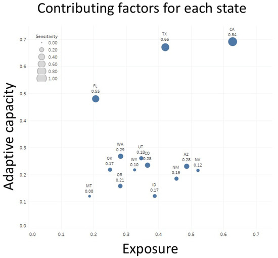
Figure 8.
Plot showing the overall contributing factors for each state, indicated by exposure (along the x axis); adaptive capacity (along the y axis); and sensitivity (denoted by the size of the circles).
Similarly, Texas has the lowest LVI of all the states analyzed. Despite its high sensitivity, its exposure to wildfire is relatively lower than more than 25% of the other states and has the second-highest adaptive capacity. Texas is highly sensitive to wildfires. According to Texas A&M Forest Service (2020), there have been over 150,000 wildfires consuming more than 9 million acres since 2005 with 71,499 wildfires in 2017 alone [50]. Indeed, 90% of wildfires in Texas are human caused as a result of debris burning, sparks from welding and grinding equipment, poorly discarded smoking materials, vehicles’ exhaust systems, and arson. Moreover, according to Headwater Economics (2018) parts of Texas that are experiencing the fastest population growth are spatially correlated with regions of highest wildfire threat and greater proportions of vulnerable people [51]. These factors contribute to the sensitivity of Texas. However, we suggest that similar to California, Texas has a very high adaptive capacity, which drastically influences its livelihood vulnerability to wildfires. This high adaptive capacity is driven primarily by social network, physical capital, and financial capital. According to the Texas A&M Forest Service (2020), Texas has resources to deploy wildfire risk information and create awareness about wildfire concerns across the state through using a Texas Wildfire Risk Assessment Portal (TxWRAP) [50]. Furthermore, data produced from this portal is part of the Texas Wildfire Risk Assessment Project (WRA) that has further positioned the Texas Forest Service as a national leader in wildfire protection planning. These resources have positioned Texas to help withstand natural hazards related to wildfires.
Additional considerations should also be taken into account for states like Arizona that exhibit a high LVI. Arizona has high exposures of wildfires and high sensitivity to environmental indices such as drought and poor air quality. According to the Arizona Commerce Authority, Arizona is among the top three states with the highest rates of population growth in the nation [52]. There have been more than 120,000 new residents (doubled California’s 50,635 new residents) in the 2018–2019 time period alone, with a projected population of over 10 million people by 2050 [52]. It can be assumed that with such growth, urbanization, transportation, and communication services will increase, thereby, making Arizona more sensitive to wildfire risk, as nine out of 10 wildland fires are started by humans according to the Arizona Department of Forestry and Fire Management [53].
We emphasize here that vulnerability is one factor in a risk assessment function, and thus, does not quantify the overall “risk”. Therefore, the resultant LVI assessment is not meant to negate the fact that California, for example, is still at high risk of wildfire impacts, but instead, provides a relative measure that compares, specifically, the aspect of livelihood vulnerability to wildfires among the 14 states. To this end, it is important that we reiterate that despite a low LVI value in California, wildfires are continuing to worsen each year causing increased casualties, significant environmental impacts, and socio-economic damages. For example, the frequency of small (less than 500 acres) of wildfires have increased predominantly across western and central California and that wildfire season is lengthening to include the month of July [54]. There are also future concerns for the state of California, despite having a low LVI. We acknowledge and emphasize that the resultant exposure to wildfire in California is the highest amongst all states, thereby requiring continuous observations and monitoring. According to [55], the increased number of fires in California is due to a combination of climate change that has heightened hot and dry conditions and fire suppression policies that have allowed the accumulation of fuels in the landscape. As stated by numerous dependencies in the California Forest Carbon Plan in 2018, wildfire emissions are projected to increase by 19%–101% using the 1961–1990 years as the baseline period [56].
If global greenhouse gas emissions continue to increase at its current rate, wildfire smoke will increase, only exacerbating these emissions and worsening the current health impacts. Therefore, looking to the future, mitigation and resiliency strategies need to be developed and adopted for the high livelihood vulnerable states, such as Arizona. In addition, continued efforts are required for relatively low LVI states that have a high exposure such as California in order to facilitate and provide resources to help mitigate wildfire hazards in the future.
The need to adopt contemporary practices is beneficial for resiliency and mitigation methods. For example, proposed policies focusing on fire suppression and prevention became prevalent in the early 1900s and represented the foundation of California’s economic theory of wildfire management, following a massive fire that had burned 3 million acres in Montana, Idaho, and Washington [57,58,59].However, according to the recent California Policy Center (2017), fire suppression techniques only worked as short-term solutions, resulting in over 100 million dead or dying trees, overgrown forests, and fuel accumulation, increasing the risk for dangerous wildland fires [60]. Thus, the continued need for evolving and enhancing fire management techniques and practices is essential for accurately monitoring and improving wildfire risk assessments.
5. Conclusions
Across the US, wildfires can produce catastrophic environmental and socio-economic impacts. To quantify these risks across multidimensional, socio-economic, and biophysical variables, we produce a framework to compute a livelihood vulnerability index for the top 14 American states that are most at risk for wildfires. Our framework comprises contributing factors (exposure, sensitivity, and adaptive capacity), major components, sub-components, and indicator variables. Our framework was further justified by performing a principal component analysis to provide additional confidence in our approach.
Our results indicate that the states of Arizona and New Mexico experience the greatest livelihood vulnerability, with an LVI of 0.57 and 0.55, respectively and California, Florida, and Texas experiencing the least livelihood vulnerability to wildfires (0.44, 0.35, 0.33, respectively). LVI is weighted strongly on the contributing factors. For example, while California has a high exposure and sensitivity to wildfires, it has high adaptive capacity capitals that offset these factors. Additionally, livelihood vulnerability depends largely on sensitivity indicator variables, such as population density. We acknowledge that, with Arizona’s high LVI and steady population growth, continued wildfire risk management and urban planning strategies are essential for reducing the biophysical and socio-economic impact of wildfires in the future and to further avoid an increase in its LVI.
This study provides a first order approximation that uses secondary (available census) data to provide a novel quantitative account of livelihood vulnerability through multidimensional factors. While we acknowledge that higher resolution scale (perhaps at the community level) would provide additional valuable information, this requires primary data acquisition through field surveys and interviews at the local scale, which is beyond the scope and feasibility of this work. However, the results generated from our relatively coarser scale analysis, can point towards high order evaluations that can be conducted at finer scales in future studies.
The results from this study are critical to researchers, government, and policymakers in identifying, allotting, and providing better resiliency and adaptation measures to support the states that are most vulnerable to wildfires. Further research can be conducted, following the same framework for each of the state’s geo-political subdivisions in order to better understand the risk and vulnerability of growing wildland–urban interface zones and to determine what urban boundary limitations should be considered for risk assessment studies. Moreover, additional research can be conducted to assess future LVI scenarios by employing high-resolution forecast models to help guide future wildland fire exposure projections in vulnerable communities within the US.
Author Contributions
Conceptualization, J.A.B.-R., M.K., M.R., K.D.T. and T.B.; methodology, J.A.B.-R., M.K., M.R., K.D.T. and T.B.; software, K.D.T.; validation, J.A.B.-R., M.K., M.R., K.D.T. and T.B.; formal analysis, J.A.B.-R., M.K., M.R. and K.D.T.; investigation, J.A.B.-R., M.K., M.R. and K.D.T.; resources, J.A.B.-R., M.K., M.R., K.D.T. and T.B.; data curation, J.A.B.-R., M.K., M.R. and K.D.T.; writing—original draft preparation, J.A.B.-R., M.K., M.R. and K.D.T.; writing—review and editing, J.A.B.-R., M.K., M.R., K.D.T. and T.B.; visualization, J.A.B.-R., M.K., M.R. and K.D.T.; supervision, T.B.; project administration, J.A.B.-R.; funding acquisition, T.B. All authors have read and agreed to the published version of the manuscript.
Funding
This research was funded by University of California, Laboratory Fees Research Program funded by the UC Office of the President (UCOP), grant number ID LFR-20-653572.
Institutional Review Board Statement
Not applicable.
Informed Consent Statement
Not applicable.
Data Availability Statement
The data presented in this study are available within the article and Table A2 in the Appendix A.
Acknowledgments
The authors would like to acknowledge the collaboration fostered from the course entitled “the science and engineering of wildfires” instructed by Professor Banerjee (T.B.) at UC Irvine, which was the impetus to this research. T.B. also acknowledges the new-faculty start-up grant provided by the Department of Civil and Environmental Engineering, and the Henry Samueli School of Engineering, University of California, Irvine.
Conflicts of Interest
The authors declare no conflict of interest.
Appendix A

Table A1.
LVI terminology definitions, color coordinated by major components in each contributing factor: adaptive capacity (green), exposure (red) and sensitivity (blue). Gray highlights denote terms that are frequently used in livelihood vulnerability literature.
Table A1.
LVI terminology definitions, color coordinated by major components in each contributing factor: adaptive capacity (green), exposure (red) and sensitivity (blue). Gray highlights denote terms that are frequently used in livelihood vulnerability literature.
| Terminology | Definition |
|---|---|
| Contributing factor | Overarching biophysical and socio-economic factors used to calculate LVI (exposure, adaptive capacity, and sensitivity) [18] |
| Adaptive capacity | The system’s (state’s) ability to adjust to a perturbation or disturbance and cope with consequences [61] |
| Exposure | The degree, time and or extent a system (state) is in contact with, or subject to a perturbation (e.g., wildfire events) [61] |
| Sensitivity | The degree to which a system (state) is modified or affected by the perturbation or set of disturbances [61] |
| Major component | The first level of divisions within each contributing factor [18] |
| Financial capital | Considers financial resources a system (state) has in order to help adapt to an exposure (wildfire) e.g., grants, income [62] |
| Human capital | Considers human resources and level of education and productive skills of people in a system (state) e.g., occupation type [62] |
| Natural capital | Considers natural resources in a system (state) that helps a system adapt to an exposure (wildfire) e.g., lakes, forests [62] |
| Physical capital | Considers materials and resources that a system (state) has to help adapt to an exposure (wildfire) e.g., transportations and communication types, infrastructure and livestock [62] |
| Social network | Considers social constructs that are in place by a system (state) in order to help adapt to an exposure (wildfire) e.g., safety practices, clubs, networks, affiliations [62] |
| Wildfire Occurrence | Metric used to quantify the number of wildland fires in a state, e.g., wildfire occurrence, loss of wildland |
| Topography | Considers metrics used to quantify topography of landscape, e.g., elevation height |
| Weather | Considers the meteorological metrics that influences wildfire behavior, e.g., air temperature |
| Weather Extreme Events | Considers metrics that quantifies extreme environmental conditions conducive for wildfires e.g., extreme heat |
| Demographic | Considers metrics that describes the population structure of a state, e.g., population density |
| Ignition causes | Considers metrics pertaining to potential ignition sources for the onset of a wildfire, e.g., smoking |
| Environment Indices | Indices that compute a potential risk related to wildfires, e.g., an air quality index |
| Subcomponent | The second level of divisions within each major component [18] |
| Indicator variables | Measurable units of data for each sub-component |
| Livelihood vulnerability index (LVI) | A vulnerability assessment tool to address issues of sensitivity, exposure and adaptive capacity to climate change (wildfire) in fire-prone communities [18] |
Table A2.
LVI framework outlining the indicator variables, sub-components, and major components that feed into each contributing factor (exposure, adaptive capacity, and sensitivity). A rationale for each indicator is provided along with a description as to how the indicator is interpreted into the LVI framework. Asterisk (*) denotes indicator variables for which the inverse values were applied in the LVI equation. In addition, the data source and the year of analysis is presented.
| EXPOSURE | ||||
|---|---|---|---|---|
| Major Components | Sub-Components | Indicator Variables and Units | Rationale and Interpretation | Date, Source and Year |
| Wildfires | Wildfire occurrence | Number of wildfires |
| Insurance Information Institute [a] (2019) |
| Loss of wildland | Total acres burnt due to wildfires in 2019 (acres) |
| National Report of Wildland Fires and Acres Burned by State (2019) [b] | |
| Topography | Elevation | Mean height above sea level (meters) |
| USGS (1980) [c] |
| Highest elevation (meters) | ||||
| Weather | Wind speed | Annual average wind speed (miles per hour) |
| NOAA Comparative Climatic Data (1950–2018) [d] |
| Relative Humidity | * Annual average Relative humidity (%) * inverse taken |
| ||
| Precipitation | * Average annual precipitation amount (inches) * inverse taken |
| ||
| * Average number of days in a year with 0.1 inch or more precipitation (days) * inverse taken |
| |||
| Temperature | Annual average temperature (℉) |
| ||
| Weather Extreme Events | Extreme wildfires | Percent of wildfires occurring between 1980 to 2010 (%) |
| World Media Group, LLC (1980–2010) [e] |
| Extreme heat | Percent of extreme heat events between 1980 to 2010 (%) |
| ||
| ADAPTIVE CAPACITY | ||||
| Major Components | Sub-Components | Indicator Variables and Units | Rationale and Interpretation | Date, Source and Year |
| Natural Capital | Forest | * Acres of forests (acres) * inverse taken |
| USDA (2016) [f] |
| Lakes/water bodies | Water area (squared miles) |
| U.S. Census Bureau, 2010 [g] | |
| Area of lakes (acres) | The Lake Almanor 2020 [h] | |||
| Physical Capital | Transportation | Miles of public road (miles) |
| Bureau of Transportation Statistics (2020) [i] |
| Number of major airports (airports) |
| |||
| Communication | Households with a computer (households) |
| U.S. Census Bureau (2014–2018) [j] | |
| Households with broadband internet connection (households) | ||||
| Human Capital | Residential density | Persons per households (persons) |
| U.S. Census Bureau (2019) [j] |
| Occupation | * Timber/wood labor (workers) * inverse taken |
| U.S. Bureau of Labor Statistics (2019) [k] | |
| Social Network | Safety | Number of Firefighters (firefighters) |
| U.S. Bureau of Labor Statistics (2019) [k] |
| Number of First responders (Emergency Medical Technicians) (EMTs) |
| U.S. Bureau of Labor Statistics (2019) [k] | ||
| Financial Capital | Income | Median household income (dollars) |
| U.S. Census Bureau (2018) [j] |
| Grant | Number of fire management assistance grants in 2017 |
| Congressional Research Service Report (2017) [l] | |
| SENSITIVITY | ||||
| Major Components | Sub-Components | Indicator Variables and Units | Rationale and Interpretation | Data Source |
| Demographic | WUI | WUI area (km2) |
| USDA (2010) [m] |
| Number of houses within WUI zones | ||||
| Population at risk in WUI Zones |
| |||
| Population | Population | U.S. Census Bureau (2019) [n] | ||
| Number of housing unit |
| U.S. Census Bureau (2019) [o] | ||
| Ignition Causes | Outdoor Activities | Number of campsites (Number) |
| Camping USA (2019) [p] |
| Smoking | Number of smokers (Millions of people) |
| America’s Health Rankings (2019) [q] | |
| Environmental Index | Index (PDI) | * Annual PDI for 2019 * inverse taken |
| NOAA_ NCEI (2019) [r] |
| Index (AQI) | Annual AQI |
| World Media Group, LLC (1999–2009) [e] | |
Data Sources for Table A2: [a] Insurance Information Institute: https://www.iii.org/fact-statistic/facts-statistics-wildfires#Wildfires%20By%20State,%202019 (accessed on 20 August 2021); [b] National Report of Wildland Fires and Acres Burned by State: https://www.predictiveservices.nifc.gov/intelligence/2019_statssumm/fires_acres19.pdf (accessed on 20 August 2021); [c] USGS Science for a changing world: https://pubs.usgs.gov/gip/Elevations-Distances/elvadist.html (accessed on 20 August 2021); [d] NOAA NCEI: https://www.ncdc.noaa.gov/ghcn/comparative-climatic-data (accessed on 20 August 2021); [e] World Media Group LLC: http://www.usa.com/ (accessed on 20 August 2021); [f] USDA 2016: https://www.fs.usda.gov/sites/default/files/fs_media/fs_document/publication-15817-usda-forest-service-fia-annual-report-508.pdf (accessed on 20 August 2021); [g] NFPA: https://www.nfpa.org/News-and-Research/Publications-and-media/Blogs-Landing-Page/NFPA-Today/Blog-Posts/2021/06/07/Types-of-Water-Supplies (accessed on 20 August 2021); [h] The Lake Almanor: https://www.uslakes.info/ (accessed on 20 August 2021); [i] Bureau of transportation: https://www.bts.gov/browse-statistical-products-and-data/state-transportation-statistics/state-transportation-numbers (accessed on 20 August 2021); [j] US Census Bureau: https://www.census.gov/quickfacts/fact/map/CA,US/HSG445218 (accessed August 2020); [k] US Bureau of labor statistics: https://data.bls.gov/oes/#/geoOcc/Multiple%20occupations%20for%20one%20geographical%20; https://www.bls.gov/ooh/protective-service/firefighters.htm#:~:text=Employment%20of%20firefighters%20is%20projected,have%20the%20best%20job%20prospects (accessed on 20 August 2021); [l] Congressional Research Service Report 2017: https://fas.org/sgp/crs/misc/R44966.pdf (accessed on); [m] USDA 2010: https://www.fs.fed.us/nrs/pubs/rmap/rmap_nrs8.pdf (accessed on 20 August 2021).; [n] US Census Bureau: https://www.census.gov/quickfacts/fact/map/CA,US/HSG445219 (accessed on 20 August 2021); [o] US Census Bureau: https://www.census.gov/quickfacts/fact/table/US/PST045219# (accessed on 20 August 2021); [p] Camping USA: https://camping-usa.com/campgrounds/ (accessed on 20 August 2021); [q] America’s Health Ranking: https://www.americashealthrankings.org/explore/annual/measure/Smoking/state/CA (accessed on 20 August 2021); [r] NOAA_NCEI: https://www.ncdc.noaa.gov/temp-and-precip/drought/nadm/indices/palmer/div#select-forms%20=%20http://www.usa.com/rank/us--air-quality-index--state-rank.htm?hl=CA&hlst=CA (accessed on 20 August 2021); [s] World Media Group, LLC: http://www.usa.com/california-state-air-quality.htm (accessed on 20 August 2021).
Table A3.
Total area (acres) burnt for each state during the 2018 and 2019 year, obtained from the Wildfire Risk Report [12].
Table A3.
Total area (acres) burnt for each state during the 2018 and 2019 year, obtained from the Wildfire Risk Report [12].
| State | Total Area Burnt in 2018 and 2019 (acres) |
|---|---|
| California | 1,823,153 |
| Nevada | 1,001,966 |
| Oregon | 897,262 |
| Oklahoma | 745,097 |
| Idaho | 604,481 |
| Texas | 569,811 |
| Colorado | 475,803 |
| Utah | 438,983 |
| Washington | 438,833 |
| New Mexico | 382,344 |
| Wyoming | 279,242 |
Table A4.
The Kaiser- Meyer-Olkin (KMO) measure of sampling adequacy and Bartlett’s Test of Sphericity results for each contributing factor of exposure, adaptive capacity, and sensitivity.
Table A4.
The Kaiser- Meyer-Olkin (KMO) measure of sampling adequacy and Bartlett’s Test of Sphericity results for each contributing factor of exposure, adaptive capacity, and sensitivity.
| Contributing Factor | Major Components | Kaiser-Meyer-Olkin Measure of Sampling Adequacy | Bartlett’s Test of Sphericity |
|---|---|---|---|
| Exposure | Wildfires Topography Weather Weather extreme events | 0.5 0.5 0.488 0.5 | 0.11 0.351 0 0.264 |
| Adaptive Capacity | Natural capital Physical capital Human capital Social network Financial capital | 0.612 0.613 0.5 0.5 0.5 | 0.101 0 0.37 0 0.434 |
| Sensitivity | Demographic Ignition causes Environmental index | 0.788 0.5 0.5 | 0 0.004 0.04 |
Table A5.
A matrix loading table, showing each indicator variable for the exposure contributing factor and its respective loading into each major component (wildfires, topography, weather, and weather extreme events).
Table A5.
A matrix loading table, showing each indicator variable for the exposure contributing factor and its respective loading into each major component (wildfires, topography, weather, and weather extreme events).
| Exposure Component Matrix | ||||
|---|---|---|---|---|
| Indicators | Wildfires | Topography | Weather | Weather Extreme Events |
| Number of wildfires | 0.85 | |||
| Number of acres burnt | 0.85 | |||
| Mean height above sea level | 0.797 | |||
| Highest elevation | 0.797 | |||
| Annual average wind speed | 0.166 | |||
| Annual average humidity | 0.968 | |||
| Annual average precipitation | 0.974 | |||
| Annual number of days with 0.1 inch or more precipitation a year | 0.748 | |||
| Annual average temperature | 0.39 | |||
| Number of extreme wildfires | 0.813 | |||
| Number of extreme heat occurrences | 0.813 | |||
Table A6.
A matrix loading table, showing each indicator variable for the adaptive capacity contributing factor and its respective loading into each major component (social network, natural, physical, human, and financial capital).
Table A6.
A matrix loading table, showing each indicator variable for the adaptive capacity contributing factor and its respective loading into each major component (social network, natural, physical, human, and financial capital).
| Adaptive Capacity Component Matrix | |||||
|---|---|---|---|---|---|
| Indicators | Natural Capital | Physical Capital | Human Capital | Social Network | Financial Capital |
| Acres of forest | −0.654 | ||||
| Water area | 0.831 | ||||
| Area of lakes | 0.847 | ||||
| Miles of public road | 0.874 | ||||
| Number of major airports | 0.964 | ||||
| Number of households with a computer | 0.981 | ||||
| Number of households with broadband internet connection | 0.977 | ||||
| Number of people per household | 0.794 | ||||
| Number of timber/wood laborers | −0.794 | ||||
| Number of firefighters | 0.998 | ||||
| Number of first responders (EMTs) | 0.998 | ||||
| Median household income | 0.783 | ||||
| Number of fire management assistance grants | 0.783 | ||||
Table A7.
A matrix loading table, showing each indicator variable for the sensitivity contributing factor and its respective loading into each major component (demographic, ignition causes, and environmental index).
Table A7.
A matrix loading table, showing each indicator variable for the sensitivity contributing factor and its respective loading into each major component (demographic, ignition causes, and environmental index).
| Sensitivity Component Matrix | |||
|---|---|---|---|
| Indicators | Demographic | Ignition Causes | Environmental Index |
| WUI area | 0.985 | ||
| Number of houses within WUI zone | 0.993 | ||
| Population at risk in WUI zones | 0.994 | ||
| Population density | 0.906 | ||
| Housing units | 0.991 | ||
| Number of camping sites | 0.926 | ||
| Number of smokers | 0.926 | ||
| Annual PDI | −0.882 | ||
| Annual AQI | 0.882 | ||
Table A8.
This table shows the original LVI value outputs for each state generated from our framework, compared to the LVI scenarios calculated when one indicator variable is omitted from the calculation under a specific major component. The symbols under some LVI represent the lowest three (---, --, -) and highest three (***, **, *) LVI value among the states.
| Indicator Variable Removed | LVI for Texas | LVI for Florida | LVI for California | LVI for Washington | LVI for Montana | LVI for Oklahoma | LVI for Wyoming | LVI for Utah | LVI for Oregon | LVI for Nevada | LVI for Colorado | LVI for Idaho | LVI for New Mexico | LVI for Arizona |
|---|---|---|---|---|---|---|---|---|---|---|---|---|---|---|
| Original | 0.3344 --- | 0.3511 -- | 0.4469 - | 0.5045 | 0.5055 | 0.5056 | 0.5107 | 0.5155 | 0.5267 | 0.5360 | 0.5372 | 0.5443 * | 0.5512 ** | 0.5717 *** |
| In Exposure without: | ||||||||||||||
| Number of wildfires | 0.3072 --- | 0.3508 -- | 0.4156 - | 0.5093 | 0.5060 | 0.5085 | 0.5139 | 0.5205 | 0.5277 | 0.5420 | 0.5462 | 0.5497 * | 0.5589 ** | 0.5803 *** |
| Mean height asl | 0.3543 --- | 0.3624 -- | 0.4822 - | 0.5093 | 0.5060 | 0.5084 | 0.5091 | 0.5036 | 0.5276 | 0.5374 | 0.5335 | 0.5447 * | 0.5519 ** | 0.5798 *** |
| Annual average wind speed | 0.3031 --- | 0.3406 -- | 0.4997 - | 0.5046 | 0.5003 | 0.4926 | 0.5060 | 0.5112 | 0.5267 | 0.5375 | 0.5326 | 0.5437 * | 0.5439 ** | 0.5776 *** |
| % of extreme heat events | 0.3547 --- | 0.3558 -- | 0.4156 - | 0.4838 | 0.5053 | 0.5043 | 0.5139 | 0.5215 | 0.5295 | 0.5304 | 0.5473 | 0.5502 * | 0.5584 ** | 0.5795 *** |
| In Sensitivity without: | ||||||||||||||
| WUI area | 0.3450 --- | 0.3506 -- | 0.4446 - | 0.5045 | 0.5056 | 0.5053 | 0.5121 | 0.5172 | 0.5275 | 0.5405 | 0.5393 | 0.5483 * | 0.5542 ** | 0.5760 *** |
| Number of campsites | 0.3260 --- | 0.3442 -- | 0.4481 - | 0.5043 | 0.5044 | 0.5061 | 0.5111 | 0.5155 | 0.5219 | 0.5405 | 0.5367 | 0.5421 * | 0.5538 ** | 0.5730 *** |
| Air quality index | 0.3269 --- | 0.3429 -- | 0.4458 - | 0.5051 | 0.5033 | 0.5040 | 0.5032 | 0.5068 | 0.5277 | 0.5219 | 0.5293 | 0.5294 * | 0.5412 ** | 0.5592 *** |
| In Adaptive Capacity without: | ||||||||||||||
| Area of lakes | 0.3525 --- | 0.3532 -- | 0.4108 - | 0.4984 | 0.5064 | 0.5062 | 0.5090 | 0.5135 | 0.5243 | 0.5360 | 0.5329 | 0.5429 * | 0.5487 ** | 0.5726 *** |
| Miles of public road | 0.3525 --- | 0.3442 -- | 0.4343 - | 0.5023 | 0.5057 | 0.5068 | 0.5090 | 0.5125 | 0.5270 | 0.5345 | 0.5366 | 0.5439 * | 0.5509 ** | 0.5693 *** |
| Persons per household | 0.3324 --- | 0.3453 -- | 0.4524 - | 0.5032 | 0.5047 | 0.5061 | 0.5097 | 0.5267 | 0.5267 | 0.5377 | 0.5371 | 0.5480 * | 0.5536 ** | 0.5758 *** |
| Number of firefighters | 0.3390 --- | 0.3553 -- | 0.4685 - | 0.5034 | 0.5047 | 0.5037 | 0.5090 | 0.5122 | 0.5255 | 0.5343 | 0.5352 | 0.5432 * | 0.5491 ** | 0.5702 *** |
| Median household income | 0.3238 --- | 0.3427 -- | 0.4685 - | 0.5213 | 0.5067 | 0.5049 | 0.5132 | 0.5246 | 0.5342 | 0.5379 | 0.5525 ** | 0.5468 | 0.5483 * | 0.5763 *** |
--- = Lowest LVI, -- = Second lowest LVI, - = Third lowest LVI, *** = Highest LVI, ** = Second highest LVI, * = Third highest LVI.
References
- Pyne, S.J. Fire: A Brief History, 2nd ed.; University of Washington Press: Seattle, WA, USA, 2019; ISBN 9780295746180. [Google Scholar]
- Román, M.V.; Azqueta, D.; Rodrígues, M. Methodological approach to assess the socio-economic vulnerability to wildfires in Spain. For. Ecol. Manag. 2013, 294, 158–165. [Google Scholar] [CrossRef]
- WHO. Climate Change and Health: On the Latest IPCC Report; Elsevier: Amsterdam, The Netherlands, 2014. [Google Scholar] [CrossRef]
- Ghorbanzadeh, O.; Blaschke, T.; Gholamnia, K.; Aryal, J. Forest fire susceptibility and risk mapping using social/infrastructural vulnerability and environmental variables. Fire 2019, 2, 50. [Google Scholar] [CrossRef] [Green Version]
- Richardson, L.A.; Champ, P.A.; Loomis, J.B. The hidden cost of wildfires: Economic valuation of health effects of wildfire smoke exposure in Southern California. J. For. Econ. 2012, 18, 14–35. [Google Scholar] [CrossRef]
- Moritz, M.A.; Batllori, E.; Bradstock, R.A.; Gill, A.M.; Handmer, J.; Hessburg, P.F.; Leonard, J.; McCaffrey, S.; Odion, D.C.; Schoennagel, T.; et al. Learning to coexist with wildfire. Nature 2014, 515, 58–66. [Google Scholar] [CrossRef] [PubMed]
- Kramer, H.A.; Mockrin, M.H.; Alexandre, P.M.; Stewart, S.I.; Radeloff, V.C. Where wildfires destroy buildings in the US relative to the wildland–urban interface and national fire outreach programs. Int. J. Wildland Fire 2018, 27, 329. [Google Scholar] [CrossRef] [Green Version]
- NOAA National Centers for Environmental Information (NCEI). U.S. Billion-Dollar Weather and Climate Disasters. 2020. Available online: https://www.ncdc.noaa.gov/billions/ (accessed on 20 August 2021).
- Westerling, A.L.; Hidalgo, H.G.; Cayan, D.R.; Swetnam, T.W. Warming and Earlier Spring Increase Western U.S. Forest Wildfire Activity. Science 2006, 313, 940–943. [Google Scholar] [CrossRef] [PubMed] [Green Version]
- Association for Fire Ecology. Reduce Wildfire Risks or We’ll Continue to Pay More for Fire Disasters. 2015. Available online: http://fireecology.org/ (accessed on 20 August 2021).
- Abatzoglou, J.T.; Williams, A.P. Impact of anthropogenic climate change on wildfire across western US forests. Proc. Natl. Acad. Sci. USA 2016, 113, 11770–11775. [Google Scholar] [CrossRef] [Green Version]
- NIFC Report 2019. Available online: https://www.nifc.gov/fireInfo/fireInfo_statistics.html (accessed on 20 August 2021).
- Calkin, D.E.; Gebert, K.M.; Jones, J.G.; Neilson, R.P. Forest Service large fire area burned and suppression expenditure trends, 1970–2002. J. For. 2005, 103, 179–183. [Google Scholar] [CrossRef]
- Baijnath-Rodino, J.A.; Foufoula-Georgiou, E.; Banerjee, T. In review. Reviewing the “hottest” fire indices worldwide. ESSOAr 2020. [Google Scholar] [CrossRef]
- Giovanni, L.; Jahjah, M.; Fabrizio, F.; Fabrizio, B. The development of a fire vulnerability index for the Mediterranean region. In Proceedings of the 2011 IEEE International Geoscience and Remote Sensing Symposium, Vancouver, BC, Canada, 24–29 July 2011; pp. 4146–4149. [Google Scholar] [CrossRef]
- Alexandre, P.M.; Stewart, S.I.; Keuler, N.S.; Clayton, M.K.; Mockrin, M.H.; Bar-Massada, A.; Syphard, A.D.; Radeloff, V.C. Factors related to building loss due to wildfires in the conterminous United States. Ecol. Appl. 2016, 26, 2323–2338. [Google Scholar] [CrossRef]
- Polsky, C.; Neff, R.; Yarnal, B. Building comparable global change vulnerability assessments: The vulnerability scoping diagram. Glob. Environ. Chang. 2007, 17, 472–485. [Google Scholar] [CrossRef]
- Hahn, M.B.; Riederer, A.M.; Foster, S.O. The Livelihood Vulnerability Index: A pragmatic approach to assessing risks from climate variability and change—A case study in Mozambique. Glob. Environ. Chang. 2009, 19, 74–88. [Google Scholar] [CrossRef]
- Etwire, P.M.; Al-Hassan, R.M.; Kuwornu, J.K.; Osei-Owusu, W. Application of livelihood vulnerability index in assessing vulnerability to climate change and variability in Northern Ghana. J. Environ. Earth Sci. 2013, 3, 157–170. [Google Scholar]
- Shah, K.U.; Dulal, H.B.; Johnson, C.; Baptiste, A. Understanding livelihood vulnerability to climate change: Applying the livelihood vulnerability index in Trinidad and Tobago. Geoforum 2013, 47, 125–137. [Google Scholar] [CrossRef]
- Chambers, R.; Conway, G.R. Sustainable Rural Livelihoods: Practical Concepts for the 21st Century; Institute of Development Studies: Brighton, UK, 1992; ISBN 0 903715 58. Available online: https://www.ids.ac.uk/publications/sustainable-rural-livelihoods-practical-concepts-for-the-21st-century/ (accessed on 20 August 2021).
- Füssel, H.-M.; Klein, R.J. Climate Change Vulnerability Assessments: An Evolution of Conceptual Thinking. Clim. Chang. 2006, 75, 301–329. [Google Scholar] [CrossRef]
- Adu, D.T.; Kuwornu, J.K.M.; Anim-Somuah, H. Application of Livelihood Vulnerability Index in Assessing Smallholder Maize Arming Households’ Vulnerability to Climate Change in Brong-Ahafo Region of Ghana. Kasetsart J. Soc. Sci. 2018, 39, 22–32. [Google Scholar] [CrossRef]
- IPCC. Climate Change 2001. Impacts, Adaptation and Vulnerability: Summary for Policymakers; Cambridge University Press: Cambridge, UK, 2001. [Google Scholar]
- Ebi, K.L.; Kovats, R.S.; Menne, B. An approach for assessing human health vulnerability and public health interventions to adapt to climate change. Environ. Health Perspect. 2006, 114, 1930–1934. [Google Scholar] [CrossRef] [Green Version]
- Albizua, A.; Corbera, E.; Pascual, U. Farmers’ vulnerability to global change in Navarre, Spain: Large-scale irrigation as maladaptation. Reg. Environ. Chang. 2019, 19, 1147–1158. [Google Scholar] [CrossRef]
- Suryanto, S.; Rahman, A. Application of livelihood vulnerability index to assess risks for farmers in the Sukoharjo Regency and Klaten Regency, Indonesia. Jàmbá J. Disaster Risk Stud. 2019, 11, 739. [Google Scholar] [CrossRef] [Green Version]
- Baijnath-Rodino, J.; Albizua, A.; Sushama, L.; Bennett, E.; Robinson, B. Determining Freshwater Lake Communities’ Vulnerability to Snowstorms in the Northwest Territories. Water 2021, 13, 1816. [Google Scholar] [CrossRef]
- Sullivan, C.A. Calculating a Water Poverty Index. World Dev. 2002, 30, 1195–1210. [Google Scholar] [CrossRef]
- O’Brien, K.; Leichenko, R.; Kelkar, U.; Venema, H.; Aandahl, G.; Tompkins, H.; Javed, A.; Bhadwal, S.; Barg, S.; Nygaard, L.; et al. Mapping vulnerability to multiple stressors: Climate change and globalization in India. Glob. Environ. Chang. 2004, 14, 303–313. [Google Scholar] [CrossRef]
- Vincent, K. Uncertainty in adaptive capacity and the importance of scale. Glob. Environ. Chang. 2007, 17, 12–24. [Google Scholar] [CrossRef]
- Thornton, P.K.; Jones, P.G.; Owiyo, T.; Kruska, R.L.; Herrero, M.T.; Kristjanson, P.M.; Notenbaert, A.M.O.; Bekele, N.; Omolo, A. Mapping Climate Vulnerability and Poverty in Africa; 2006. [Google Scholar]
- Rengers, F.K.; McGuire, L.A.; Oakley, N.S.; Kean, J.W.; Staley, D.M.; Tang, H. Landslides after wildfire: Initiation, magnitude, and mobility. Landslides 2020, 17, 2631–2641. [Google Scholar] [CrossRef]
- Syphard, A.D.; Radeloff, V.C.; Keeley, J.E.; Hawbaker, T.J.; Clayton, M.K.; Stewart, S.I.; Hammer, R.B. Human influence on california fire regimes. Ecol. Appl. 2007, 17, 1388–1402. [Google Scholar] [CrossRef]
- Li, S.; Dao, V.; Kumar, M.; Nguyen, P.; Banerjee, T. Mapping the wildland-urban interface in CA using remote sensing data. ESSOAr 2021. [Google Scholar] [CrossRef]
- Gannon, B.; Roberts, J. Social capital: Exploring the theory and empirical divide. Empir. Econ. 2018, 58, 899–919. [Google Scholar] [CrossRef] [Green Version]
- Keeley, J.E.; Syphard, A.D. Twenty-first century California, USA, wildfires: Fuel-dominated vs. wind-dominated fires. Fire Ecol. 2019, 15. [Google Scholar] [CrossRef] [Green Version]
- Banerjee, T. Impacts of Forest Thinning on Wildland Fire Behavior. Forests 2020, 11, 918. [Google Scholar] [CrossRef]
- Wotton, B.M. Interpreting and using outputs from the Canadian Forest Fire Danger Rating System in research applications. Environ. Ecol. Stat. 2008, 16, 107–131. [Google Scholar] [CrossRef]
- Lund, A.; Lund, M. How to Perform a Principal Components Analysis (PCA) in SPSS Statistics|Laerd Statistics. 2018. Available online: Statistics.laerd.com. (accessed on 13 July 2020).
- Williams, B.; Onsman, A.; Brown, T. Exploratory factor analysis: A five-step guide for novices. Australas. J. Paramedicine 2010, 8. [Google Scholar] [CrossRef] [Green Version]
- Tobias, S.; Carlson, J.E. Brief report: Bartlett’s test of sphericity and chance findings in factor analysis. Multivar. Behav. Res. 1969, 4, 375–377. [Google Scholar] [CrossRef] [PubMed]
- Kaiser, H.F. A second generation little jiffy. Psychometrika 1970, 35, 401–415. [Google Scholar] [CrossRef]
- Storey, M.A.; Price, O.F.; Sharples, J.J.; Bradstock, R.A. Drivers of long-distance spotting during wildfires in south-eastern Australia. Int. J. Wildland Fire 2020, 29, 459. [Google Scholar] [CrossRef]
- Davies, I.P.; Haugo, R.D.; Robertson, J.C.; Levin, P.S. The unequal vulnerability of communities of color to wildfire. PLoS ONE 2018, 13, e0205825. [Google Scholar]
- Wuensch, K.L. Principal Components Analysis-SPSS; 2012. [Google Scholar]
- Zach. A Guide to Bartlett’s Test of Sphericity. Statology. 2019. Available online: https://www.statology.org/bartletts-test-of-sphericity/ (accessed on 13 July 2020).
- Yong, A.G.; Pearce, S. A Beginner’s Guide to Factor Analysis: Focusing on Exploratory Factor Analysis. Tutorials Quant. Methods Psychol. 2013, 9, 79–94. [Google Scholar] [CrossRef]
- California State Budget, 2019–2020. Available online: http://www.ebudget.ca.gov/2019-20/pdf/Enacted/BudgetSummary/FullBudgetSummary.pdf (accessed on 20 August 2021).
- Texas A&M Forest Service Texas A&M Forest Service. Available online: https://www.texaswildfirerisk.com/About (accessed on 20 August 2021).
- Headwater Economics. 2018. Available online: https://headwaterseconomics.org/wp-content/uploads/Austin-Full-Report.pdf (accessed on 20 August 2021).
- Arizona Commerce Authority. Available online: https://www.azcommerce.com/oeo/population/population-projections/ (accessed on 20 August 2021).
- Arizona Department of Forestry and Fire Management (DFFM). Available online: https://dffm.az.gov/blog-terms/fire (accessed on 20 August 2021).
- Li, S.; Banerjee, T. Spatial and temporal pattern of wildfires in California from 2000 to 2019. Sci. Rep. 2021, 11, 1–17. [Google Scholar] [CrossRef]
- Miller, R.K.; Field, C.B.; Mach, K.J. Barriers and enablers for prescribed burns for wildfire management in California. Nat. Sustain. 2020, 3, 101–109. [Google Scholar] [CrossRef]
- California Forest Carbon Plan in 2018. Available online: https://resources.ca.gov/CNRALegacyFiles/wp-content/uploads/2018/05/California-Forest-Carbon-Plan-Final-Draft-for-Public-Release-May-2018.pdf (accessed on 20 August 2021).
- Silcox, F.A. Fire Prevention and Control on the National Forests. From the Yearbook of Department of Agriculture for 1910. 1910. Available online: https://foresthistory.org/wp-content/uploads/2017/01/Silcox_Fire_1910.pdf (accessed on 20 August 2021).
- Headley, R. Fire Suppression, District 5; United States Forest Service: Washington, DC, USA, 1916; 57p. Available online: https://www.srs.fs.usda.gov/pubs/40193 (accessed on 1 August 2021).
- Rideout, D.B.; Wei, Y.; Kirsch, A.G.; Botti, S.J. Toward a Unified Economic Theory of Fire Program Analysis with Strategies for Empirical Modeling. In The Economics of Forest Disturbances; Springer: Dordrecht, The Netherland, 2008; pp. 361–380. [Google Scholar] [CrossRef]
- California Policy Center. Long-Term Solutions for California Wildfire Prevention. 2017. Available online: https://californiapolicycenter.org/long-term-solutions-for-california-wildfire-prevention/ (accessed on 20 August 2021).
- Gallopin, G.C. Linkages between vulnerability, resilience, and adaptive capacity. Glob. Environ. Chang. 2006, 16, 293–303. [Google Scholar] [CrossRef]
- Dulal, H.B.; Brodnig, G.; Onoriose, C.G.; Takur, H.K. Capitalizing on Assets: Vulnerability and Adaptation of Climate Change in Nepal; Social Development Working Papers, No. 121; The World Bank: Washington, DC, USA, 2010. [Google Scholar]
- National Wildfire Coordinating Group. Available online: https://www.nwcg.gov/sites/default/files/training/docs/s-190-student-workbook.pdf (accessed on 20 August 2021).
- Kumar, M.; Li, S.; Nguyen, P.; Banerjee, T. Revisiting the existing definitions of wildland-urban interface for California. ESSOAr 2020. [CrossRef]
- National Wildfire Coordinating Group. Fire Behavior. 1981. Available online: http://www.auburn.edu/academic/forestry_wildlife/fire/ (accessed on 20 August 2021).
- USDA. 2003. Available online: https://www.fs.fed.us/projects/hfi/2003/november/documents/forest-structure-wildfire.pdf (accessed on 20 August 2021).
- NFPA. Available online: https://www.nfpa.org/News-and-Research/Publications-and-media/Blogs-Landing-Page/NFPA-Today/Blog-Posts/2021/06/07/Types-of-Water-Supplies (accessed on 20 August 2021).
- CAL Fire Fuel Breaks and Use during Fire Suppression, CAL Fire, 2019. Available online: https://www.fire.ca.gov/media/5585/fuel_break_case_studies_03212019.pdf (accessed on 20 August 2021).
- Firefighting Aircraft, Recognition Guide. Available online: https://www.fire.ca.gov/media/4950/aviation-guide-2019-access.pdf (accessed on 20 August 2021).
- Newsom, D.; Herzenberg, C.; Swieltik, C. Value of the Internet in emergency response. In IPCC 99. Communication Jazz: Improvising the New International Communication Culture. In Proceedings of the 1999 IEEE International Professional Communication Conference, New Orleans, LA, USA, 7–10 September 1999; IEEE: Piscataway, NJ, USA, 2003. [Google Scholar] [CrossRef] [Green Version]
- Shouse Injury Law Group. 2021. Available online: https://www.shouselaw.com/ca/personal-injury/good-samaritan-law/ (accessed on 20 August 2021).
- The Oregonian, 2020. Available online: https://www.oregonlive.com/wildfires/2020/11/after-the-fires-timber-industry-faces-generational-losses-and-longer-term-supply-questions-of-supply.html (accessed on 20 August 2021).
- Occupational Outlook Handbook: US Bureau of Labor Statistics. Available online: https://www.bls.gov/ooh/protective-service/firefighters.htm#:~:text=Employment%20of%20firefighters%20is%20projected,have%20the%20best%20job%20prospects. (accessed on 20 August 2021).
- Employment Development Department State of California, 2021. Available online: https://www.labormarketinfo.edd.ca.gov/OccGuides/Detail.aspx?Soccode=292041&Geography=0604000107#:~:text=In%20California%2C%20the%20number%20of,growth%20rate%20for%20all%20occupations.&text=for%20all%20occupations.,Jobs%20for%20Emergency%20Medical%20Technicians%20and%20Paramedics%20are%20expected%20to,jobs%20between%202018%20and%202028 (accessed on 20 August 2021).
- Socioeconomic Factors and the Incidence of Fire, FEMA. 1997. Available online: https://www.usfa.fema.gov/downloads/pdf/statistics/socio.pdf (accessed on 20 August 2021).
- Fire Prevention and Safety, FEMA, 2021. Available online: https://www.fema.gov/grants/preparedness/firefighters/safety-awards#awards (accessed on 20 August 2021).
- Scott, J.H.; Gilbertson-Day, J.; Stratton, R.D. 2019. Available online: http://pyrologix.com/wp-content/uploads/2019/11/RiskToCommunities_OR-WA_BriefingPaper.pdf (accessed on 20 August 2021).
- Butry, D.T.; Prestemon, J.P.; Thomas, D.S. Investigation of the decline in reported smoking-caused wildfires in the USA from 2000 to 2011. Int. J. Wildland Fire 2014, 23, 790–798. [Google Scholar] [CrossRef] [Green Version]
- North American Drought Monitor. Available online: https://www.ncdc.noaa.gov/temp-and-precip/drought/nadm/indices/palmer/div#select-form (accessed on 20 August 2021).
- World Media Group LLC. Available online: http://www.usa.com/ (accessed on 20 August 2021).
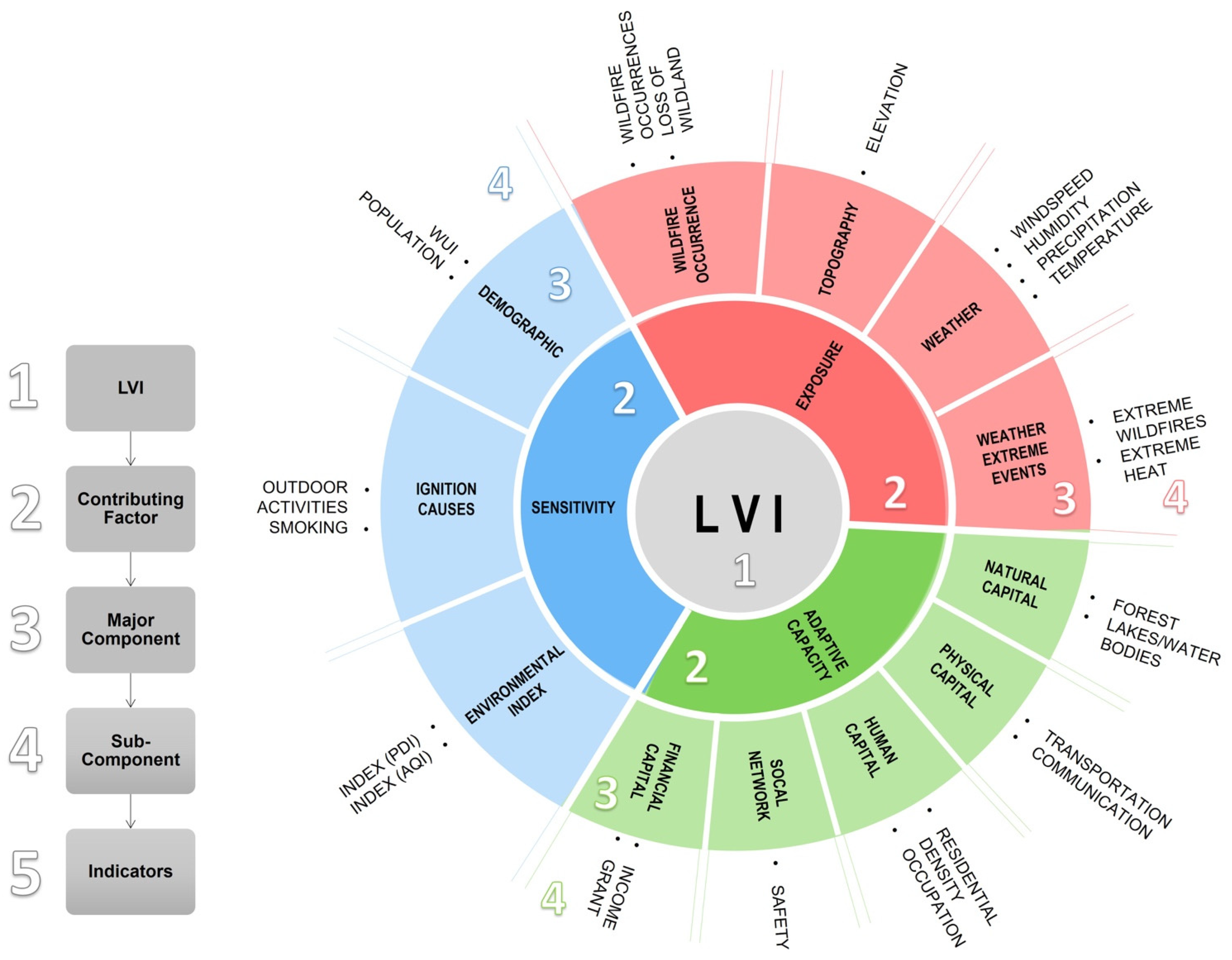


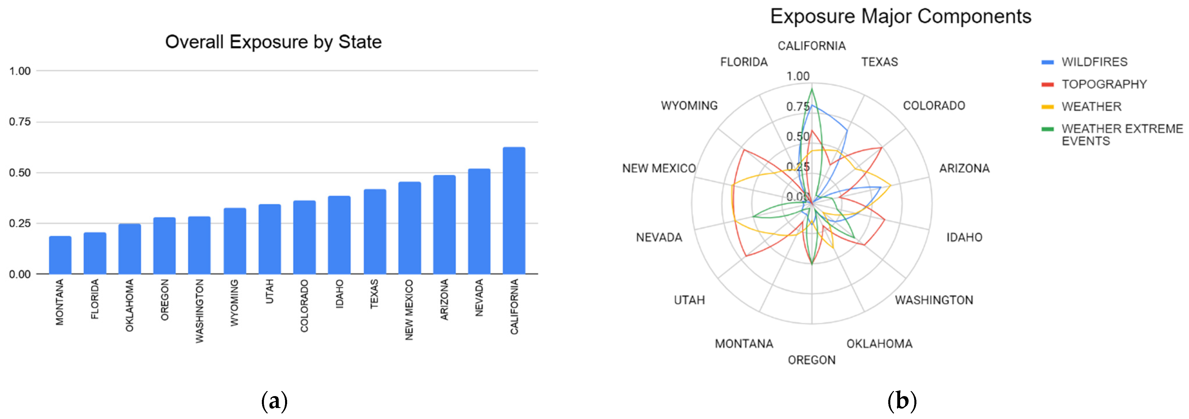


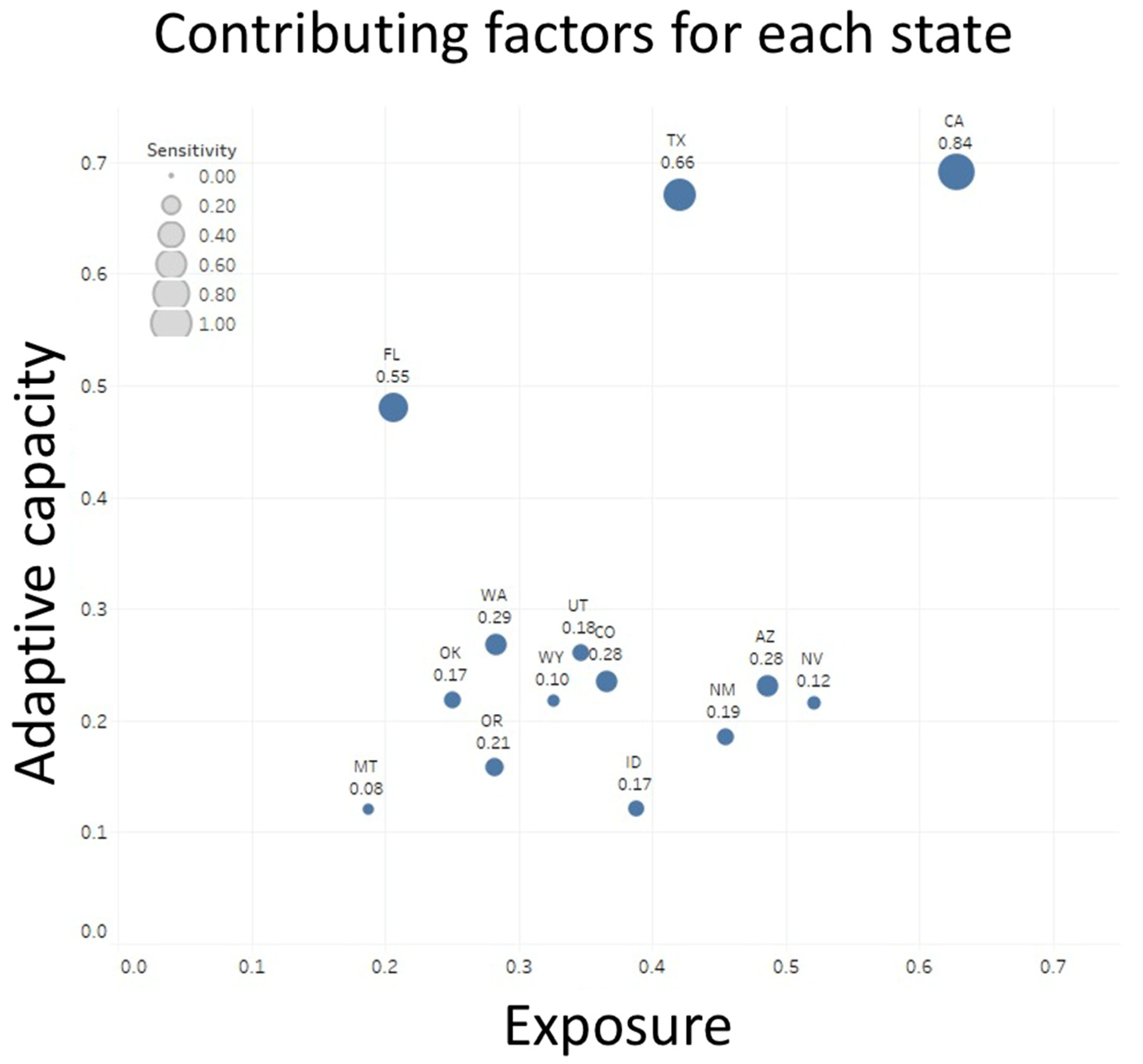
Publisher’s Note: MDPI stays neutral with regard to jurisdictional claims in published maps and institutional affiliations. |
© 2021 by the authors. Licensee MDPI, Basel, Switzerland. This article is an open access article distributed under the terms and conditions of the Creative Commons Attribution (CC BY) license (https://creativecommons.org/licenses/by/4.0/).