Article

Comparative Assessment of Wildland Fire Rate of Spread Models: Effects of Wind Velocity

by
Dionysios I. Kolaitis
*,
Christos Pallikarakis
and
Maria A. Founti
School of Mechanical Engineering, National Technical University of Athens, 15772 Athens, Greece
*
Author to whom correspondence should be addressed.
Fire 2023, 6(5), 188; https://doi.org/10.3390/fire6050188
Submission received: 27 March 2023 / Revised: 26 April 2023 / Accepted: 2 May 2023 / Published: 4 May 2023
(This article belongs to the Special Issue Dynamics of Wind-Fire Interaction: Fundamentals and Applications)

Abstract

:
Wildland fire rate of spread prediction models are important tools for the effective coordination of resident evacuation and fire suppression efforts. A comparative assessment of ten empirical and semi-empirical rate of spread prediction models is performed, using a selection of 203 laboratory experiments of surface spreading fires; special emphasis is given to the effects of external wind velocity. Five of the evaluated models have been developed using measurements obtained in laboratory-scale tests; these models are combined with two supplementary sub-models that account for the effects of wind. In addition, a selection of five empirical models that have been developed using large-scale field tests are also assessed. The performance of the ten prediction models is evaluated, both qualitatively and quantitatively, by employing a range of statistical error metrics. The laboratory-developed models are found to exhibit high sensitivity on low fuel load values, when no external wind is present, as well as on low packing ratios and high wind velocity values. The field-developed models exhibit significant discrepancies against the experimental data, due to the use of specific parameters regarding fuel type, scale and wind velocity.

1. Introduction

Wildland fires may have a devastating impact on society and the natural environment. In this context, the study of wildland fires has the aim of providing detailed information on the physical and chemical phenomena, spanning multiple spatial and temporal scales, that characterise the respective initiation, spreading and suppression mechanisms. The prediction of the wildland fire rate of spread (ROS) is important, since knowledge of the spatial–temporal evolution of a wildland fire front provides valuable information for a broad range of activities, ranging from fire defence to civilian evacuation. Due to the complexity of the phenomena involved, along with the requirements for faster-than-real-time predictions, various approaches [1,2,3] have been developed to model and predict the wildland fire ROS.
The two main modelling methodologies that are extensively used in operational environments are the “empirical” and the “semi-empirical” approach. These models comprise simple mathematical equations that yield a “quasi-steady state” value of ROS (R), as a function of relevant parameters for fuel, atmosphere and topography characteristics. Both approaches utilise empirical data, originating from either small-scale laboratory experiments or large-scale field tests, such as experiments, prescribed burns or actual wildland fire events. Semi-empirical models are based upon an energy balance equilibrium; however, they do not distinguish among the different modes of heat transfer, as “physical” models do. On the other hand, empirical models are essentially statistical correlations, connecting the empirical data to the ROS. Nevertheless, physical reasoning may not be absent from empirical modelling, since the selection of the functional forms that mathematically describe a parameter’s effect on ROS is commonly based on previous theoretical analyses. It has been shown [4] that the appropriate selection of functional forms can result in successful model extrapolation beyond the range of the specific empirical data used for model development. Both empirical and semi-empirical approaches present, due to their intended simplicity, a range of inherent limitations. One of the most important limitations is the fact that they commonly neglect the dynamic behaviour of the fire, which is known to change with time, even when the boundary conditions regarding the fuel, atmosphere and topography parameters remain the same [5].
Due to the various macroscopic forms that a natural environment can manifest, e.g., forests, grasslands, woodlands, etc., specific empirical and semi-empirical models have been developed for different environments. In this context, “surface” ROS prediction models are utilised in environments where aerial fuel is absent; the existence of a canopy adds complexity to the behaviour of the fire. Furthermore, even among the broad range of surface fuels available, the respective models may be focused on either “generic” surface fuel types or a “specific” fuel type. Generic surface-fuel-type models are usually developed using laboratory data, which are characterised by a well-defined and controllable experimentation process but represent the wildland fire phenomena at a reduced scale. On the contrary, specific-fuel models are commonly developed using field data, which represent the phenomenon at its real scale, while lacking the experimental control of laboratory tests.
Among the various atmospheric properties that influence a wildland fire’s ROS, wind velocity is of particular significance. This is mainly due to its dynamic behaviour, since the magnitude or direction of the wind may change constantly. Wind velocity is incorporated into the majority of ROS models, either directly, as a specific parameter, or indirectly, through a “wind correction” sub-model that specifically accounts for the effects of wind and is used to “modify” the predicted ROS value for quiescent conditions. It is common for field-developed models to directly incorporate the effects of wind velocity, since quiescent wildland fires are generally characterised by relatively low ROS values, compared to fires spreading under external wind conditions.
In this study, a selection of laboratory and field-developed models, as well as wind correction sub-models, are evaluated against laboratory data of surface fires found in the open literature. The main purpose of this work is to comparatively assess the performance of the laboratory-developed models combined with the supplementary wind models, as well as the field-developed models, against well-controlled laboratory experiments, aiming to evaluate their ability to yield ROS values with acceptable accuracy. Similar validation studies have been performed in the past, such as a qualitative comparison of laboratory- and field-developed models against laboratory data with the effect of wind and slope combined [6]; a quantitative comparison of laboratory-based models against laboratory data on live vegetation fuel, again, with the aforementioned effects combined [7]; a broad collection of validation studies of field-developed models against field data [8]; as well as a quantitative comparison of laboratory- and field-developed models against laboratory data under the presence of wind [9]. In this context, the current work is mainly focused on the quantitative comparison of several contemporary laboratory- and field-developed models against a broad range of laboratory-scale surface fires, with a special emphasis on the effect of wind velocity on their prediction quality.

2. Materials and Methods

In this work, a selection of five laboratory-developed, generic surface fuel ROS prediction models, along with two wind correction sub-models, and a selection of five field-developed fuel-specific models are assessed against laboratory experimental data found in the open literature. The laboratory-developed models are the well-known semi-empirical models of Rothermel [10], its re-examination from Wilson [11] and the model of Catchpole et al. [12], as well as two empirical models of Rossa and Fernandes [13]. The wind correction sub-models are the empirical correction factor of Rothermel [10] and the empirical wind model of Rossa and Fernandes [14]. The investigated field-developed empirical models are the model of Burrows et al. [15], the models of Anderson et al. [16], the model of Fernandes et al. [17], as well as the Canadian Forest Fire Behaviour Prediction System (CFFBPS) [18]. The general form of each model is presented in Table 1, while the respective detailed equations, values of the various parameters and a description of all symbols are given in the Appendix A and Appendix B.

2.1. Semi-Empirical, Laboratory-Developed ROS Models

The semi-empirical models of Rothermel (L1), Wilson (L2) and Catchpole et al. (L3) are based on the theoretical work of Frandsen [19], presented in 1971. In Frandsen’s work, the steady-state ROS (R) of an (infinite-width) advancing flaming front was expressed (Equation (1)) as the ratio of the heat flux transferred from the burning front to the unburned fuel, i.e., the propagating heat flux (IP), over the heat per unit volume required by the fuel volume to ignite (Lig).
R = I P L i g
In 1972, Rothermel [10] advanced Frandsen’s concept to a fully operational model; the proposed model is considered a “milestone” in the field of wildland fire science. Rothermel’s model focuses primarily on the “fundamental” physical mechanisms of fire spread due to the fuel characteristics, while the effects of wind and slope are considered to be “secondary”, treating them in a purely empirical manner. More specifically, the model introduces the concept of reaction intensity (IR) which corresponds to the heat flux generated from the fire front; in this case, the propagating heat flux (IP) is a fraction of IR, defined as the propagating heat flux ratio (ξ). Through mathematical manipulation, assumptions and theoretical reasoning, the model expresses the ROS under quiescent and horizontal conditions (R0) as a function of physical properties that can be measured, calculated or correlated to measured fuel parameters through laboratory experimentation (c.f. Table A1).
In 1990, Wilson [11] proposed a reformulation of Rothermel’s model, based on an extended set of laboratory experimental data and using different assumptions and theoretical reasoning compared to the original model. The two main new concepts of Wilson’s model are that, on the one hand, the reaction intensity (IR) only originates from the flaming combustion of the fire front, and, on the other hand, fuel ignition initiates when the fuel pyrolysis is completed. In addition, Wilson proposed different functional forms and property dependencies on IR and ξ (c.f. Table A2).
The model of Catchpole et al. [12] is a semi-empirical model, also based in the original work of Frandsen, developed from wind-tunnel experimentation. In contrast to the previously presented models, this model does not consider the effect of wind as a “secondary” effect, but instead, it incorporates wind effects directly to the propagation heat flux (IP). The latter, in this case, is not expressed as the product of IR·ξ, but it is directly empirically correlated to the fuel characteristics, as well as to wind velocity. It is noted that the functional form for the wind velocity correction can also yield results for the case of quiescent conditions. Moreover, the L3 model keeps the proposal of Wilson [11] on the onset of fuel ignition after the completion of pyrolysis. Finally, this model considers the effect of fuel bed width (W) by means of a proportional multiplier of R for fuel beds that have a width lower than 1 m.

2.2. Empirical, Laboratory-Developed ROS Models

The two laboratory-developed, empirical models investigated in this work are the models proposed by Rossa and Fernandes [13]. The authors presented a couple of empirical models for the prediction of the “base” (i.e., quiescent conditions and flame propagation on a horizontal terrain) ROS on dead and alive generic surface fuels. Both models (L4 and L5) consider the effects of fuel moisture content (M) and fuel bed depth (δ), while the second model (L5) also accounts for the effect of specific surface (s), a quantity that corresponds to the ratio of surface area-to-volume ratio (σ) over the fuel element particle density (ρp).

2.3. Wind Correction Empirical Sub-Models

Wind correction sub-models are essentially supplementary models that specifically account for the additional effects of wind; they are commonly applied to the ”base” ROS (R0) models, aiming to “correct” their values for wind effects. The wind correction sub-model of Rothermel [10] (W1) makes use of a correction factor (ΦW), which is estimated from laboratory experiments and is empirically correlated to the wind velocity (U) and to other fuel and fuel bed parameters (c.f. Table A3). The dependence of ΦW on the fuel characteristics is associated with the physical observation that when the fuel bed is less compact, heat transfer from the burning front to the fuel bed is more efficient and vice versa in the case of a closely packed fuel bed.
Rossa and Fernandes developed an empirical sub-model (W2) to account for the effects of wind [14]; despite its empirical nature, it is based on physical reasoning in an attempt to describe the change in fire spread mechanisms under the effect of wind. The model recognises that one of the major effects of external wind on the flame front is the modification of the angle between the flame and the unburned fuel bed. For quiescent conditions, the flame tends to tilt backwards (upstream) due to increased air entrainment from the downstream direction, induced by the asymmetric temperature field, upstream and downstream of the flame front. In this case, fuel heating due to flame radiation is less important compared to radiation from the burning fuel bed. When external wind is present, the flame front is “pushed” towards the unburnt fuel, decreasing the angle between them, thus resulting in an increased contribution of the flame radiation heating. Radiation heating depends on the emissivity and the temperature of the flame envelope, as well as the envelope’s height and relative angle with the unburnt fuel bed. Thus, an increase in wind velocity results in an increase in the heat transfer rate from the flame to the unburnt fuel, and by extension, an increase in the observed ROS (c.f. Equation (1)). However, according to Byram [20], and as shown in Equation (2), an increase in ROS results in an increase in the fireline intensity (IB), which is an alternative expression for the energy generated, similar to IR. Subsequently, an increase in IB implies the increasing momentum of the buoyant plume behind the fire front, which tends to pull the flame away from the unburned fuel bed, thus decreasing the above-mentioned flame geometry characteristics (height and angle) and the contribution of flame radiation heating. Thus, external wind initiates a “competition” between the pushing of the flaming front towards the fuel bed and the pulling of the flaming front by the buoyant plume whose strength is increased, indirectly, by the wind. By assuming that the momentum of the buoyant plume is analogous to the rate that the fuel is added to the flame ( m ˙ ), the W2 model introduces a correction factor (RU) that is empirically correlated to the wind velocity (U), m ˙ and the ratio of fuel bed to flame height (δ/Hf)0; the latter parameter quantifies the flame extension above the fuel bed. The model assumes that m ˙ = m·R0, while the (δ/Hf)0 parameter is empirically estimated as a function of FMC (c.f. Table A4), based on a previous work of Rossa and Fernandes [21].
IB = h·m·R

2.4. Empirical, Field-Based Models and Wind Adjustment Factor

The remaining five empirical models (F1–F5) have been developed using field experiments or observational studies of actual wildland fires on specific flora environments. Burrows et al. [15] modelled the flame ROS on spinifex grassland, a horizontally discontinuous surface fuel, yielding a “parsimonious” three-parameter model (F1). Anderson et al. [16] presented a group of empirical models (F2 and F3) based on a large database of shrubland fires. Fernandes et al. [17] developed a model for predicting the flame ROS on maritime pine stands (F4). Lastly, the Forestry Canada Fire Danger Group [18] developed the Fire Behaviour Prediction (FBP) System from various types of field experiments and observational studies (F5). This model has been developed to accept fuel-specific parameters from various fuel models of Canadian flora environments (c.f. Table A5).
The nominal velocity required as an input by the various field-developed ROS prediction models may differ due to the wind velocity profile developing in the Atmospheric Boundary Layer (ABL). In the ABL, the axial wind velocity decreases with decreasing height. As a result, the wind velocity measured at a given height above the flame may be significantly higher than the wind velocity close to the flame, which is the region where the external wind directly affects the flame front. On the other hand, in laboratory experiments, the velocity profile in a wind tunnel depends on the characteristics of the wind tunnel itself; in this case, the nominal velocity usually refers either to the “free stream velocity” of a developing flow or the “mean velocity” of a fully developed flow. Due to the limited wind tunnel dimensions, the reference velocity is a better approximation of the wind velocity that, being close to the fire front, is directly affecting it. Therefore, in order to use the field-developed models to predict ROS values obtained in laboratory tests, the wind tunnel velocity needs to be adjusted to an “equivalent” velocity that corresponds to the actual height that atmospheric wind velocity is measured as for each model. This wind velocity “adjustment” is performed using the methodology proposed by Albini and Baughman [22], where the Wind Adjustment Factor (WAF) is introduced. The latter parameter corresponds to the ratio of the wind velocity at mid-flame height ( U ¯ ¯ ) to the atmospheric velocity measured at height z (Uz). The Wind Adjustment Factor is estimated using Equation (3) [23] and is formulated under the assumption that the flame height above the fuel bed is considered to be approximately equal to the height of the fuel bed [24].
W A F = U ¯ ¯ U z = 1.83 ln z + 0.36 δ 0.13 δ
The adjustment of the wind tunnel velocity (U) to the atmospheric velocity measured at height z (Uz) is based on the additional assumption that the wind tunnel nominal velocity, due to the scale of the laboratory fires, is approximately equal to U ¯ ¯ , an assumption that is commonly made in studies of similar nature [6].

2.5. Laboratory Experimental Data

The ten investigated ROS models (L1–L5 and F1–F5) and the two wind correction sub-models (W1 and W2) were evaluated against a broad set of fuel bed surface fire laboratory experiments, available in the open literature [25,26,27,28,29]. More specifically, 203 individual fire tests were used to assess the prediction accuracy of the investigated models and model combinations; 166 of these fire tests were performed under the effect of external wind, whereas the remaining 37 fire tests corresponded to quiescent wind conditions. The specific set of experimental data used in this study was selected due to the fact that the respective research works either present all the parameters required by the investigated ROS models or allow for an estimation of these parameters through inferences and reasonable assumptions. A brief summary of the main characteristics of the fire tests used for the validation study is given in Table 2.
Due to inconsistencies between the required model input parameters and the information available on the laboratory tests, a number of assumptions had to be made. The fuel chemical properties, such as fuel heat content (h) and the heat content of the volatile gases (hv) needed in the L1 and L2 models, respectively, were assumed to be 18,608 and 12,306 kJ/kg, respectively, based on information presented in references [6,10]. The heat of pyrolysis (QP), the moisture damping constant (k) and the equivalent characteristic moisture content (Mc) required for models L2 and L3 were taken from [12], based on the specific fuel type of each fire test. The moisture of extinction (Mx), the total mineral content (ST) and the effective mineral content (Se), needed for the calculation of IR,1 of model L1, were assumed to be equal to 0.3, 0.0555 and 0.01, respectively, based on [10]. The parameter n ¯ x required for the L2 model was assumed to be equal to 3, according to [11]. For the wind correction model W2, (fil) was assumed to be 2.42 [14]. In terms of the F1 model, the fuel cover parameter (CF) was assumed to be equal to 1, since the fuel beds used in the experiments had a “continuous” fuel distribution. For certain fuel properties, i.e., h, St, Se, Mx, hv and fil, a sensitivity analysis was performed, aiming to investigate the impact of their assumed values on the respective model performance.
Finally, for the F5 model, the C-6 fuel type was selected [18]. In terms of the FMC and the fuel load values reported in the respective experimental works, they were assumed to be on a “dead” basis, unless otherwise reported or inferred. Finally, due to the fact that the σ and ρp parameters of the Pinus Pinaster needles that were used in [25] were not reported, they were assumed to be equal to 3057 m−1 and 511 kg/m3, respectively; these values were taken from laboratory tests performed on the same fuel [30,31]. The assumptions that were made in order to be able to use all the investigated models for all the considered fire tests (c.f. Table A6) may have affected, to a certain degree, the accuracy of the predicted ROS values.

3. Results

The performance of the investigated models against the selected set of laboratory experiments is assessed both qualitatively and quantitatively, by comparing the level of agreement of the “predicted” ROS values with the respective “measured” ROS values. The results are quantitatively evaluated by calculating the values of several statistical error metrics. The error metrics selected are the Mean Biased Error (MBE), the Mean Absolute Percentage Error (MAPE) and the Root Mean Square Error (RMSE) [17]. The magnitude and sign of the MBE indicate the tendency of the model to under- or over-predict the experimental data. The magnitude of the MAPE indicates the tendency of the model to diverge from the observed values, while being a metric of the scattering of the results. The magnitude of the RMSE provides similar information to that of the MAPE but shows higher sensitivity to large discrepancies. The formulas of the above error metrics are presented in Equations (4)–(6), where Rpred and Rexp are the predicted and measured ROS values, respectively, and n is the total number of experiments.
RMSE = 1 n R exp R p r e d 2 n 1 2
MAPE = 1 n R exp R p r e d R exp n 100 %
MBE = 1 n R p r e d R exp n
Initially, the performance of the five laboratory-developed models (L1–L5) against the 37 no-wind laboratory tests is presented, followed by the performance of the ten laboratory-developed model/wind correction sub-model combinations (L-W) against the 166 fire tests with external wind. Then, the performance of the five field-developed models (F1–F5) against the external wind fire tests is presented; since the equations of these models cannot provide a ROS value for zero wind velocity, it was not possible to assess their performance against the no-wind fire tests. Finally, a sensitivity analysis focused on the assumed values for six characteristic model fuel properties is presented, aiming to investigate their impact on the prediction accuracy of the respective models.

3.1. Laboratory-Developed Models in Quiescent Conditions

In Figure 1, ROS predictions of the five laboratory-developed models are compared against the respective measured values, obtained in the 37 fire tests performed in quiescent conditions; the bold dashed line corresponds to “perfect agreement”, whereas the normal dashed lines represent the ±35% “acceptable” error intervals, as proposed in [4]. In general, the under-prediction of the measured ROS values is undesirable, especially when the respective model is used in actual operational environments. It is evident that the obtained predictions exhibit significant scatter; however, the majority of the predicted values lie within the ±35% error region. The L1 model shows a tendency for under-prediction, while the L2 model exhibits a slight tendency for over-prediction. The L3 model under-predicts the measured ROS values in the low region (R < 2 mm/s). Models L4 and L5 demonstrate relatively good prediction qualities.
The corresponding error metric values for all 37 no-wind fire tests considered are presented in Table 3; text in bold corresponds to the minimum values for each error metric. The calculated error metrics agree with the aforementioned qualitative observations. For all the 37 no-wind test cases, the L1 model exhibits the larger negative MBE, while the L3 model exhibits the highest positive MBE and the highest RMSE and MAPE; this is mainly attributed to a group of highly over-predicted values (c.f. Figure 1). The L4 and L5 models present the lowest RMSE and MBE values, whereas their MAPE values are quite close to that of L1. Overall, based on the error metrics matrix, both L4 and L5 models exhibit the best prediction quality among the five investigated models.
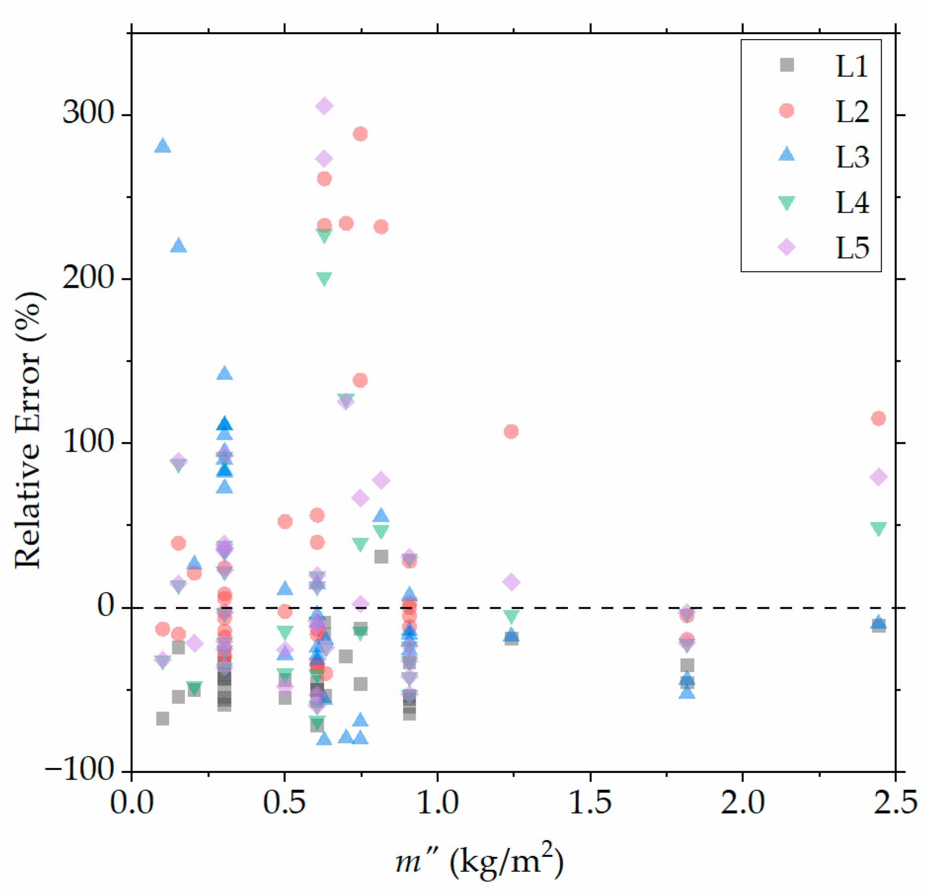
Aiming to investigate the potential impact of certain physical parameters on the prediction quality of the investigated ROS models, the relative error of the predicted values is presented in Figure 2, as a function of the (dry) fuel load (m) for all the considered test cases. It is evident that the scatter of the predicted values is reduced with increasing fuel load, thus suggesting high sensitivity of the ROS models to relatively low fuel load values. Among the five ROS models, the L3 model exhibits higher sensitivity in low m values, thus resulting in the relatively high error values reported in Table 1.

3.2. Laboratory-Developed Models, Combined with Wind-Correction Sub-Models, against External Wind Conditions

In Figure 3, predictions of the laboratory-developed models (L1–L5) combined with the two wind correction sub-models (W1 and W2) are compared against the respective measured values in the 166 fire tests with external wind.
The two wind correction models exhibit relatively different behaviours. The performance of W1 depends strongly on the ROS model that it is applied to. More specifically, model W1 has a tendency for under-prediction when applied to the L1 and L4 models, while, when applied to the L2 and L3 models, the W1 model tends to yield results that over-predict the measurements. When applied to model L5, the W1 correction yields the most accurate results. On the contrary, the W2 wind correction model does not exhibit a strong dependence on the underlying ROS model. It is evident that the W2 model yields highly over-predicted values, especially in the region of high ROS values (R > 100 mm/s).
In Table 4, the error metrics for all model combinations are presented. The absolute values of all calculated error metrics are generally higher than the respective values obtained for the no-wind cases (c.f. Table 3), thus echoing the increased difficulty in accurately predicting the ROS of a wildland fire in the presence of external wind. It is evident that the W1 wind correction model performs, in all cases, better than the W2 model. In general, lower error values are observed when the W1 sub-model is combined with models L1, L4 and L5; this is expected, since these specific models also yield the best results in the no-wind test cases (c.f. Table 3). Overall, the combination with the lowest error metrics is L5-W1.
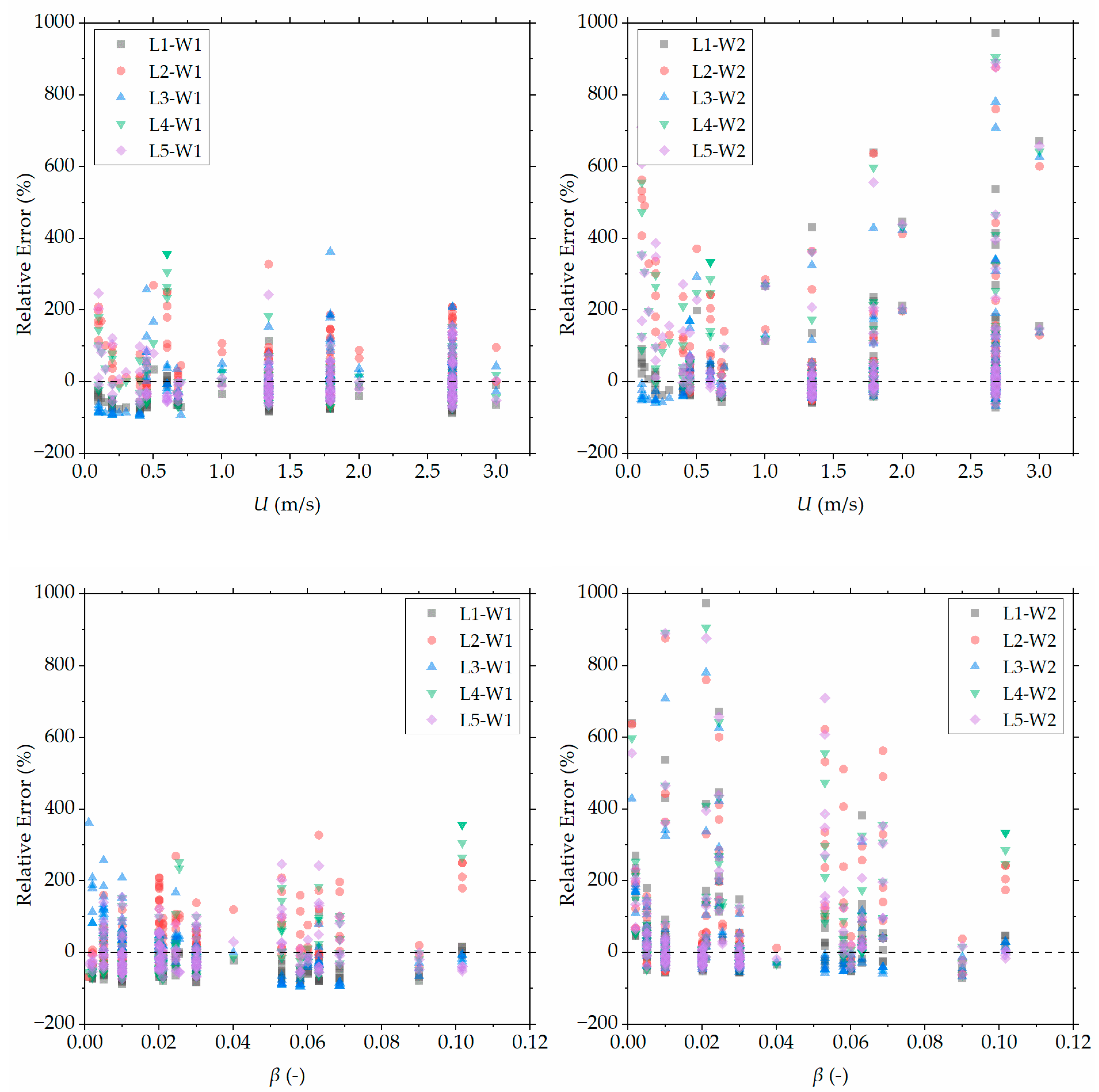
Aiming to further investigate the impact of certain physical parameters on the prediction accuracy of the investigated models, the calculated relative error for all ten model combinations is presented in Figure 4 as a function of wind velocity (Figure 4, top) and packing ratio (Figure 4, bottom). It is evident that an increase in wind velocity results in an overall decrease in the prediction accuracy of model W2, while W1 seems to be unaffected. Moreover, the accuracy of W2 is decreased at very low wind velocities. Regarding the effect of packing ratio, it seems to have no effect in W1, while it tends to decrease the accuracy of W2 with decreasing β.

3.3. Field-Developed Models against External Wind Conditions

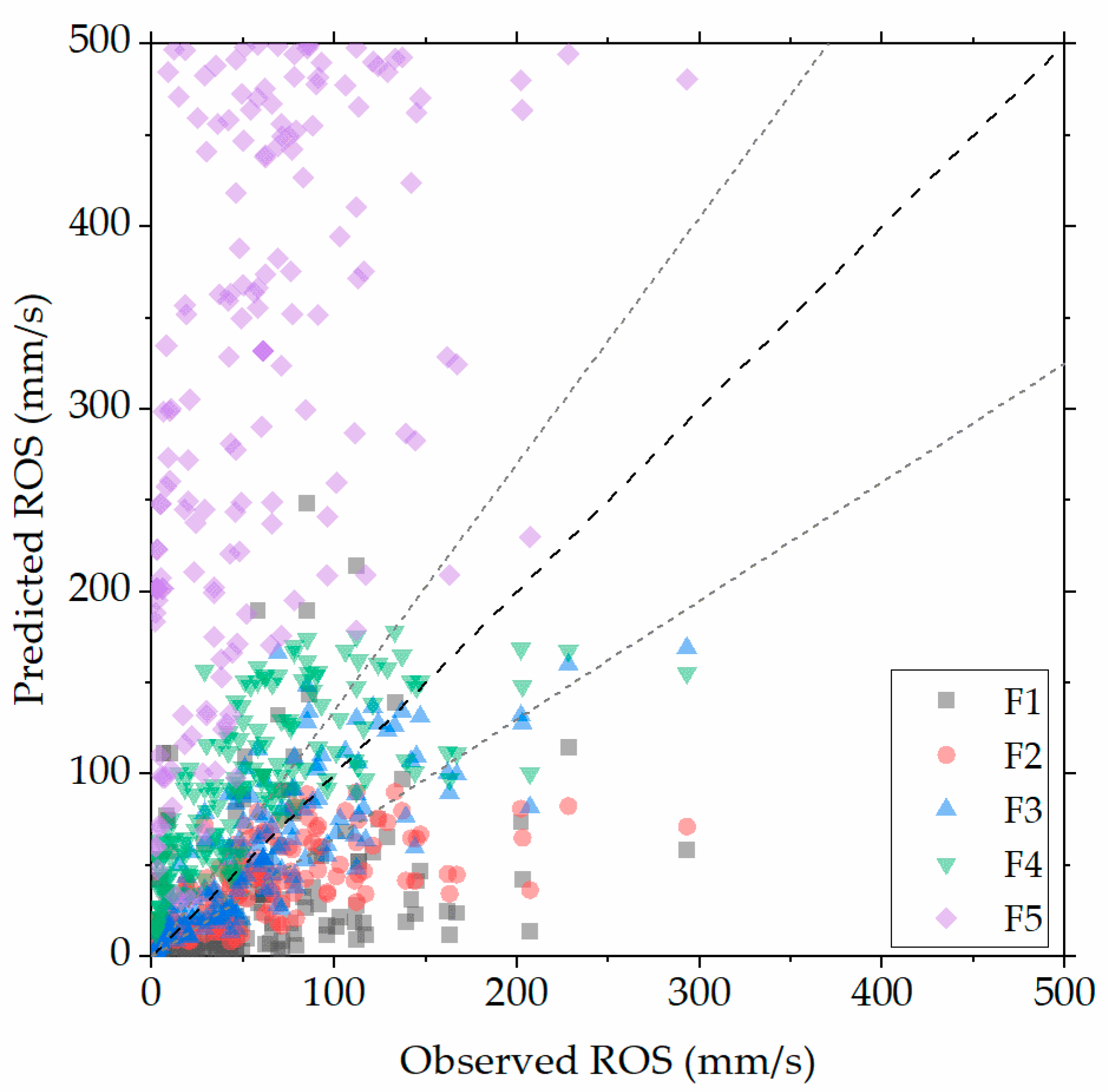
In Figure 5, ROS predictions using the field-developed models are compared to the respective measured values for the 166 test cases where external wind was present. In general, the predictions are significantly more scattered compared to the respective results of the laboratory-developed models obtained for the same fire tests (c.f. Figure 3). This is expected, since the field-developed models are strongly dependent on the specific fuel type used in the corresponding field tests, thus making their good performance in fire tests in which different fuel types are used quite a challenge. The F1 model significantly under-predicts the measured values, whereas the F5 model exhibits the strongest over-prediction. Model F4 is also slightly over-predicting. Model F2 shows a slight tendency for under-prediction, compared to that of model F1, while the F3 model results exhibit relatively smaller discrepancies.
The calculated error metrics for the five field-developed models against all 166 wind fire tests are presented in Table 5. The significant over-prediction tendency of model F5 is evident, since the respective error metric values are very high. The lowest error metrics are obtained when the F3 model is used; however, these values are generally higher than the respective values obtained using the laboratory-developed models (c.f. Table 4). The large scatter of the majority of the field-developed models (c.f. Figure 5) is reflected in the generally large MBE values.

3.4. Sensitivity Analysis

A sensitivity analysis was performed, aiming to investigate the impact of the selected values for certain model parameters on the prediction accuracy of the respective models. Six model parameters were considered in this study, namely the fuel heat content (h), the total (St) and effective (Se) mineral content and the moisture of extinction (Mx) of model L1; the fuel’s pyrolysis gas lower calorific value (hv) for model L2; and the ignition line length factor (fil) used in wind correction W2. Towards this end, the value of each parameter was varied by ±25%; these variation limits were selected as an adequate representation of the “common” value range of the corresponding specific fuel properties. The results of the sensitivity analysis are presented in Table 6, in the form of the change in the overall RMSE values when each parameter value was changed by ±25%. It is evident that variations in the fuel heat content (h) used in model L1, the fuel’s pyrolysis gas lower calorific value (hv), used in model L2, as well as the ignition line length factor (fil) used in model W2 (the model combination L5-W2 was used for the sensitivity analysis), result in moderate sensitivity of the obtained prediction accuracy, whereas the rest of the fuel parameters have less significant impacts. The relatively higher sensitivity on the h, hv and fil parameter values is expected, since the h and fil parameters are essentially “multipliers” in the respective ROS equations (c.f. Table 1), whereas hv is an additional input through a more complicated functional form. Overall, the calculated sensitivity of the investigated parameters is considered to be reasonable, since their assumed values do not have an unexpected strong influence on the obtained results.

4. Discussion

The overall quality of the obtained predictions suggests the inherent complexities associated with the accurate description of wildland fire ROS, due to the interacting complex physical phenomena that span a broad range of spatial and temporal scales.
In the absence of wind, the main characteristics affecting the ROS of a surface fire seem to be sufficiently described by available ROS models, since the majority of the investigated models yielded relatively accurate results. The best prediction quality was achieved by model L5; notably, this is the most recently developed model, having been introduced in 2018 [13]. This suggests the importance of continuously updating ROS models by constantly incorporating the latest research findings, with the aim of improving the available operational tools. The empirical model of Rossa and Fernandes (L5) suggests that, in the absence of wind, the effects of fuel bed characteristics can be better described by the fuel bed height (δ), whereas the effects of the fuel particles are better predicted by means of the specific surface parameter (s). In general, empirical models do not provide an in-depth insight into the nature of the occurring phenomena. On the contrary, the importance of the three semi-empirical models (L1, L2 and L3) rests in the fact that they mathematically describe the concepts of energy required for fuel ignition, energy generation from the fire front and energy transferred to the unburnt fuel, which have been shown to be the main physical/chemical processes that govern the wildland fire dynamics [32], and that the complexity of the wildland fire behaviour eventually lies in their interaction as well as their interdependence. In any case, due to the relatively small number of fire tests obtained in quiescent conditions (37), it is believed that a larger pool of experimental data would allow for an improved assessment of the relevant performance of the investigated models.
When external wind was present, the wind correction sub-model W1 yielded, in general, lower metric errors than sub-model W2. This is attributed to the different physical reasoning that the two wind correction models are based upon, regarding the effects of wind velocity and packing ratio. Sub-model W2 is mainly focused on the changes in the mechanism of radiative heat transfer under the effect of wind. In low-wind-velocity conditions, the effects of radiative heating are more pronounced than convective heating; however, at higher wind velocities, it has been proposed [33] that the mechanisms of fire spread change and the effects of convective heating become significant. In the W2 sub-model, the effects of convection are incorporated by means of the empirically fitted parameters A7 or B7 (c.f. Table 1); thus, there is less focus on the potential changes in convective heat transfer. This may be one reason for the increasing discrepancies exhibited by W2’s predictions with increasing wind velocity values (c.f. Figure 4). On the other hand, in the very low wind velocity region, the observed W2 discrepancies may be attributed to the fact that when the wind correction parameter RU tends to zero, the predicted ROS value is largely affected by the parameter fil (c.f. Table 1), thus leading to the potential over-prediction of the experimentally determined values. The effects of packing ratio are only taken into account by sub-model W1. The packing ratio value affects both radiation and convection; closed-packed beds are both blocking the radiation to the fuel bed’s bottom layer and decreasing the ventilation through the fuel bed. Thus, the packing ratio may be an important parameter that has to be included in generic ROS models that account for the effects of wind.
The field-developed ROS models exhibited rather divergent performances. The majority of field models showed strong tendencies for the over-prediction or under-prediction of the measured values, with the exception of the F3 model which yielded results of comparable accuracy with the most accurate laboratory-developed model-wind correction sub-model combinations. A similar observation was reported by Cruz et al. [8], where the model of Anderson et al. was also found to exhibit relatively low MBE and MAPE values against field data. It is noted that the F3 model is the only field-developed model that accounts for the effect of fuel bed width; this may have affected the achieved levels of prediction accuracy, since the laboratory tests used for the comparative study were all performed in fuel beds that exhibited typical width values significantly lower than the large-scale fires used for the development of the F models. Furthermore, F3 is the only field-developed model that includes ρb as an input. It is interesting to note that ρb (or, more specifically, its dimensionless form (β)) was shown to be affecting the prediction accuracy of the L-W model combinations. Thus, it may be the case that the effect of the fuel bed compactness, described by means of the ρb or β parameters, is an important descriptive quantity that can be closely connected to the impact of external wind on fire spreading.
In any case, the difficulty of using the field-based models to accurately predict the experimentally determined ROS values may be attributed to the following four characteristics. Firstly, field-developed models are fuel specific, which means that few fuel-related parameters are required as an input, while the rest of the parameters are integrated in various statistically fitted coefficient values. For example, the F1 model was developed using measurements obtained in spinifex grassland, a fuel that exhibits horizontal discontinuity; this fact may explain the strong tendency of this specific model to under-predict the laboratory measurements obtained in continuous fuel beds. Secondly, the fact that field experiments almost always employ “live” as well as “dead” fuels may not allow one to properly consider the effects of FMC. Thirdly, field experiments usually employ fuel areas exhibiting fuel bed width at least an order of magnitude higher compared to laboratory tests. Under external wind conditions, ROS depends on the flame front’s width, which can significantly change with time, due to the large dimensions of the fuel area in conjunction with the wind that can change both in magnitude and direction, as was observed and inferred by [34,35]. From the selected field-developed models, only the models of Anderson et al. (F2 and F3) incorporated the effects of width, and their good performance, compared with the rest of the F models, might be attributed to this fact. Finally, the assumption used to determine the WAF, i.e., that the height of the flame above the fuel bed is considered to be equal to the height of the fuel bed, is usually not valid in small-scale laboratory fires, a fact that might induce further deviations from the observed values. It is noted that similar arguments regarding the potential reasons for the observed over-predictions are reported by Weise and Biging [6] in the frame of a comparative evaluation of field-developed models tested against laboratory data.

5. Conclusions

A validation study of a selection of laboratory- and field-developed ROS models and wind corrections was performed against a set of laboratory experimental data. For the models that were developed using well-controlled laboratory experiments, it was shown that while new empirical models yield better results, the semi-empirical models provide insight into the physical mechanisms that govern the wildland fire spread phenomena. The impact of external wind velocity on ROS values was found to be affected by the fuel bed’s packing ratio, since the wind correction sub-model W1, which incorporates the packing ratio, was found to yield overall better results. The ROS models developed using large-scale field tests were, mainly, fuel-specific; therefore, they were generally not able to yield accurate results when tested against laboratory-scale fire tests. This was due to the differences in scale regarding both fuel and wind characteristics, in addition to the nature of the specific fuel type used in each test that affected the model’s empirically fitted parameters.

Author Contributions

Conceptualisation, D.I.K.; methodology, D.I.K. and C.P.; formal analysis, C.P.; investigation, C.P.; resources, D.I.K. and M.A.F.; writing—original draft preparation, C.P.; writing—review and editing, D.I.K.; supervision, M.A.F.; project administration, D.I.K. and M.A.F.; funding acquisition, M.A.F. All authors have read and agreed to the published version of the manuscript.

Funding

This research received no external funding.

Institutional Review Board Statement

Not applicable.

Informed Consent Statement

Not applicable.

Data Availability Statement

Data sharing not applicable.

Conflicts of Interest

The authors declare no conflict of interest.

Nomenclature

SymbolUnitsDescription
A, B, , F-Empirically fitted constants or functions
a, b, c-Fuel parameters, used in model F5
FC%Surface fuel cover
fil-Ignition line length factor, used in sub-model W2
HfmFlame height
hkJ/kgFuel lower calorific value
hvkJ/kgFuel’s pyrolysis gas lower calorific value
IBkW/mByram’s fireline intensity
IPkW/m2Propagation heat flux
IRkW/m2Reaction intensity
ISI-Initial Spread Index, used in model F5
k-Moisture damping constant, used in model L3
LigkJ/m3Heat per unit volume required for ignition
M*-Fuel moisture content—FMC (dry basis)
Mc-Characteristic moisture, used in model L2
Mx-Moisture of extinction, used in model L1
m ˙ kg/s·mRate of fuel added to combustion zone
mnkg/m2Net fuel load
mdkg/m2Dry fuel load
nx-Extinction index
n ¯ x -Extinction adjustment factor
n-Total number of experiments
Pf-Probability function for fire extinction
QpkJ/kgHeat of pyrolysis
QwkJ/kgRequired heat to evaporate the fuel’s moisture
R0m/s*“Base” ROS in quiescent and horizontal conditions
Rm/s*Rate of spread
Rexpm/s*Experimentally measured rate of spread
Rpredm/s*Predicted rate of spread
Ru-Wind correction factor, used in sub-model W2
Se-Effective mineral content
St-Total mineral content
sm2/kgFuel particle specific surface
Ta°CAmbient temperature
Um/s*Wind velocity
Uzm/s*Wind velocity measured at height z
U ¯ ¯ m/s*Wind velocity at mid-flame height
WmFuel bed width
zft*Wind velocity measuring height
β-Fuel bed packing ratio
Γ′min−1Potential reaction velocity
δmFuel bed height
ε-Effective heating number
ηΜ-Moisture damping coefficient
ηS-Mineral damping coefficient
ξ-Propagating heat flux ratio
ρbkg/m3Fuel bed density
ρpkg/m3Fuel particle density
σm−1Surface area-to-volume (SAV) ratio
Φw-Wind correction factor, used in sub-model W1
* Properties may, in certain cases, be expressed in different units (see text). Numerical subscripts (in Table 1, Table A1, Table A2 and Table A6) indicate different constant or function.

Appendix A. Detailed Forms of Equation Functions

The detailed form of the various functions appearing in the equations presented in Table 1, for ROS models L1, L2 and L3, F5 and the wind-correction sub-models W1 and W2 are given below.
Table A1. Detailed form of L1 model functions.
FunctionUnits
I R , 1 = Γ m n h η M , 1 η S (kJ/min·m2)
Γ = β 0.20395 σ 0.8189 exp 1 β 0.20395 σ 0.8189 1 6.7229 σ 0.1 7.27 0.0591 + 2.926 σ 1.5 (min−1)
m n = m 1 S T (kg/m2)
η M , 1 = 1 2.59 M M X + 5.11 M M X 2 3.52 M M X 3
η S = 0.174 S e 0.19
ξ 1 = e 0.792 + 3.7597 σ 0.5 β + 0.1 192 + 7.9095 σ
L 1 = ρ b ε 581 + 2594 M (kJ/m3)
ε = e 4.528 σ
σ(cm−1)
Table A2. Detailed form of L2 and L3 model functions.
FunctionUnits
ξ 2 = 1 e 0.17 σ β
L 2 = ρ b ε Q p + M Q w (kJ/m3)
I R , 2 = Γ 2 m h v η M , 2 (kJ/min·m2)
Γ 2 = 0.34 σ σ β δ 1 2 e σ β 3 P f n x (min−1)
P f n x = 1 1 + e π n x n ¯ x 1.2 3
n x = ln σ β δ h v / Q w M + Q p Q w
η M , 2 = e k M
I P , 3 = 495.5 + 1934 U 0.91 e 800 σ β 0.501 η Μ , 2 (kW/m2)
σ(cm−1)
Table A3. Detailed form of W1 model function.
FunctionUnits
Φ W = 7.47 e 0.8711 σ 0.55 3.281 0.15988 σ 0.54 β 0.20395 σ 0.8189 0.715 e 0.01094 σ U 0.15988 σ 0.54
Table A4. Detailed form of W2 model function.
FunctionUnits
δ H f 0 = 0.1779 + 3.713 10 3 M
Table A5. Detailed form of F5 model function.
FunctionUnits
I S I = A 12 e B 12 U z C 12 e D 12 M 1 + E 12 M F 12
Uz(km/h)

Appendix B. Values of Empirical Parameters

The specific values of the various empirical parameters used in each model are provided in Table A6.
Table A6. Values of empirical parameters.
ModelParameterValueModelParameterValue
L4, L5A40.2859F1A840.982
A50.1557B81.399
B4,5−0.7734C81.201
C4,50.9440D81.699
D50.8173F2, F3A95.6715
W2A72.143 × 10−5B90.9102
B71.710C90.2227
C7−1.169D90.0762
D7−1.166A103.8320
F5α45B101.0927
b0.0305C10−0.2098
c2D100.0721
A120.208E9,109
B120.05039F9,100.00316
C1291.9F4A110.773
D12−0.1386B110.707
E124.93 × 10−7C11−0.039
F125.31D110.188

References

  1. Sullivan, A.L. Wildland surface fire spread modelling, 1990–2007. 1: Physical and quasi-physical models. Int. J. Wildland Fire 2009, 18, 349–368. [Google Scholar] [CrossRef]
  2. Sullivan, A.L. Wildland surface fire spread modelling, 1990–2007. 2: Empirical and quasi-empirical models. Int. J. Wildland Fire 2009, 18, 369–386. [Google Scholar] [CrossRef]
  3. Sullivan, A.L. Wildland surface fire spread modelling, 1990–2007. 3: Simulation and mathematical analogue models. Int. J. Wildland Fire 2009, 18, 387–403. [Google Scholar] [CrossRef]
  4. Cruz, M.G.; Alexander, M.E. Uncertainty associated with model predictions of surface and crown fire rates of spread. Environ. Modell. Softw. 2013, 47, 16–28. [Google Scholar] [CrossRef]
  5. Viegas, D.X. On the existence of a steady state regime for slope and wind driven fires. Int. J. Wildland Fire 2004, 13, 101–117. [Google Scholar] [CrossRef]
  6. Weise, D.R.; Biging, G.S. A Qualitative comparison of fire spread models incorporating wind and slope effects. Forest Sci. 1997, 43, 170–180. [Google Scholar] [CrossRef]
  7. Weise, D.R.; Koo, E.; Zhou, X.; Mahalingam, S.; Morandini, F.; Balbi, J.H. Fire spread in chaparral-a comparison of laboratory data and model prediction in burning live fuels. Int. J. Wildland Fire 2016, 25, 980–994. [Google Scholar] [CrossRef]
  8. Cruz, M.G.; Alexander, M.E.; Sullivan, A.L.; Gould, J.S.; Kilinc, M. Assessing improvements in models used to operationally predict wildland fire rate spread. Environ. Modell. Softw. 2018, 105, 54–63. [Google Scholar] [CrossRef]
  9. Kolaitis, D.I.; Pallikarakis, C.N.; Founti, M.A. Effects of wind velocity on prediction of wildland fire rate of spread models: A comparative assessment using surface fuel fire tests. In Proceedings of the IX International Conference on Forest Fire Research, Coimbra, Portugal, 14–18 November 2022. [Google Scholar]
  10. Rothermel, R.C. A Mathematical Model for Predicting Fire Spread in Wildland Fuels; Res. Pap. INT-115; USDA Forest Service, Intermountain Forest and Range Experiment Station: Fort Collins, CO, USA, 1972. [Google Scholar]
  11. Wilson, R.A. Reexamination of Rothermel’s Fire Spread Equations in No-Wind and No-Slope Conditions; Res. Pap. INT-434; USDA Forest Service, Intermountain Research Station: Fort Collins, CO, USA, 1990. [Google Scholar]
  12. Catchpole, W.R.; Catchpole, E.A.; Butler, B.W.; Rothermel, R.C.; Morris, G.A.; Latham, D.J. Rate of spread of free-burning fires in woody fuels in a wind tunnel. Combust. Sci. Technol. 1998, 131, 1–37. [Google Scholar] [CrossRef]
  13. Rossa, C.G.; Fernandes, P.M. Empirical modeling of fire spread rate in no-wind and no-slope conditions. Forest Sci. 2018, 64, 358–370. [Google Scholar] [CrossRef]
  14. Rossa, C.G.; Fernandes, P.M. An empirical model for the effect of wind on fire spread. Fire 2018, 1, 31. [Google Scholar] [CrossRef]
  15. Burrows, N.; Gill, M.; Sharples, J. Development and validation of a model for predicting fire behaviour in spinifex grasslands of Arid Australia. Int. J. Wildland Fire 2019, 27, 271–279. [Google Scholar] [CrossRef]
  16. Anderson, W.R.; Cruz, M.G.; Fernandes, P.M.; McCaw, L.; Vega, J.A.; Bradstock, R.A.; Fogarty, L.; Gould, J.; McCarthy, G.; Marsden-Smedley, J.B.; et al. A generic, empirical-based model for predicting rate of fire spread in shrublands. Int. J. Wildland Fire 2015, 24, 443–460. [Google Scholar] [CrossRef]
  17. Fernandes, P.M.; Botelho, H.S.; Rego, F.C.; Loureiro, C. Empirical modelling of surface fire behavior in maritime pine stand. Int. J. Wildland Fire 2009, 18, 698–710. [Google Scholar] [CrossRef]
  18. Forest Canada Fire Danger Group. Development and Structure of the Canadian Forest Fire Behavior Prediction System; Information Report St-X-3; Forestry Canada, Science and Sustainable Development Directorate: Ottawa, Canada, 1992. [Google Scholar]
  19. Frandsen, W.H. Fire spread through porous fuels from conservation of energy. Combust. Flame 1971, 16, 9–16. [Google Scholar] [CrossRef]
  20. Byram, G.M. Combustion of Forest Fuels; McGraw-Hill: New York, NY, USA, 1959; pp. 61–89. [Google Scholar]
  21. Rossa, C.G.; Fernandes, P.M. Fuel-related fire-behaviour relationships for mixed live and dead fuels burned in the laboratory. Can. J. Forest. Res. 2017, 47, 883–889. [Google Scholar] [CrossRef]
  22. Albini, F.A.; Baughman, R.G. Estimating Windspeeds for Predicting Wildland Fire Behavior; Res. Pap. INT-221; USDA Forest Service, Intermountain Forest and Range Experiment Station: Ogden, UT, USA, 1979. [Google Scholar]
  23. Andrews, P.L. Modeling Wind Adjustment Factor and Midflame Wind Speed for Surface Fire Spread Model; Gen. Tech. Rep; RMRS-GTR-266; U.S. Department of Agriculture, Forest Service, Rocky Mountain Research Station: Ogden, UT, USA, 2012. [Google Scholar]
  24. Baughman, R.G.; Albini, F.A. Estimating Midflame Windspeed; Northern Forest Fire Laboratory: Missoula, MT, USA, 1980; pp. 88–92. [Google Scholar]
  25. Mendez-Lopez, J.M.; Ventura, J.M.; Amaral, J.M.P. Flame characteristics, temperature-time curves, and rate of spread in fires propagating in a bed of Pinus Pinaster needles. Int. J. Wildland Fire 2003, 12, 67–84. [Google Scholar] [CrossRef]
  26. Lozano, J.; Tachajapong, W.; Pan, H.; Swanson, A.; Kelley, C.; Princevac, M.; Mahalingam, S. Experimental investigation of the velocity field in a controlled wind-aided propagating fire using particle image velocimetry. In Proceedings of the Fire Safety Science-Proceedings of the 9th International Symposium, University of Karlsruhe, Karlsruhe, Germany, 21–26 September 2008; pp. 255–266. [Google Scholar]
  27. Anderson, W.R.; Catchpole, E.A.; Butler, B.W. Convective heat transfer in fire spread through fine fuel beds. Int. J. Wildland Fire 2010, 19, 284–298. [Google Scholar] [CrossRef]
  28. Korobenichev, O.; Tereshchenko, A.; Paletsky, A.; Shmakov, A.; Gonchikzhapov, M.; Chernov, A.; Kataeva, L.; Maslennikov, D.; Liu, N. The velocity and structure of the flame front at spread of fire across thepne needle bed depending on the wind velocity. In Proceedings of the 10th Asia-Oceania Symposium on Fire Science and Technology, Tsukuba, Japan, 5–7 October 2014; pp. 771–779. [Google Scholar]
  29. Korobeinichev, O.; Kumaran, S.M.; Shanmugasundaram, D.; Raghavan, V.; Trubachev, S.A.; Paletsky, A.A.; Shmakov, A.G.; Glaznev, R.K.; Chernov, A.A.; Tereshchenko, A.G. Experimental and numerical study of flame spread over bed of pine needles. Fire Technol. 2022, 58, 1227–1264. [Google Scholar] [CrossRef]
  30. Morandini, F.; Perez-Ramirez, Y.; Tihay, V.; Santoni, P.; Barboni, T. Radiant, convective and heat release characterization of vegetation fire. Int. J. Therm. Sci. 2013, 70, 83–91. [Google Scholar] [CrossRef]
  31. Tihay, V.; Morandini, F.; Santoni, P.A.; Perez-Ramirez, Y.; Barboni, T. Combustion of forest litters under slope condition: Burning rate, heat release rate, convective and radiant fractions for different loads. Combust. Flame 2014, 161, 3237–3248. [Google Scholar] [CrossRef]
  32. Finney, M.A.; McAllister, S.S.; Grumstrup, T.P.; Forthofer, J.M. Wildland Fire Behavior: Dynamics, Principles and Processes; CSIRO Publishing: Melbourne, Australia, 2021; pp. 15–45. [Google Scholar]
  33. Morvan, D.; Frangieh, N. Wildland fires behaviour: Wind effect versus Byram’s convective number and consequences upon the regime of propagation. Int. J. Wildland Fire 2018, 27, 636–641. [Google Scholar] [CrossRef]
  34. Cheney, N.P.; Gould, J.S.; Catchpole, W.R. The influence of fuel, weather and fire shape variables on fire-spread in grasslands. Int. J. Wildland Fire 1993, 3, 698–710. [Google Scholar] [CrossRef]
  35. Cheney, N.P.; Gould, J.S. Fire growth in grassland fuels. Int. J. Wildland Fire 1995, 5, 237–247. [Google Scholar] [CrossRef]
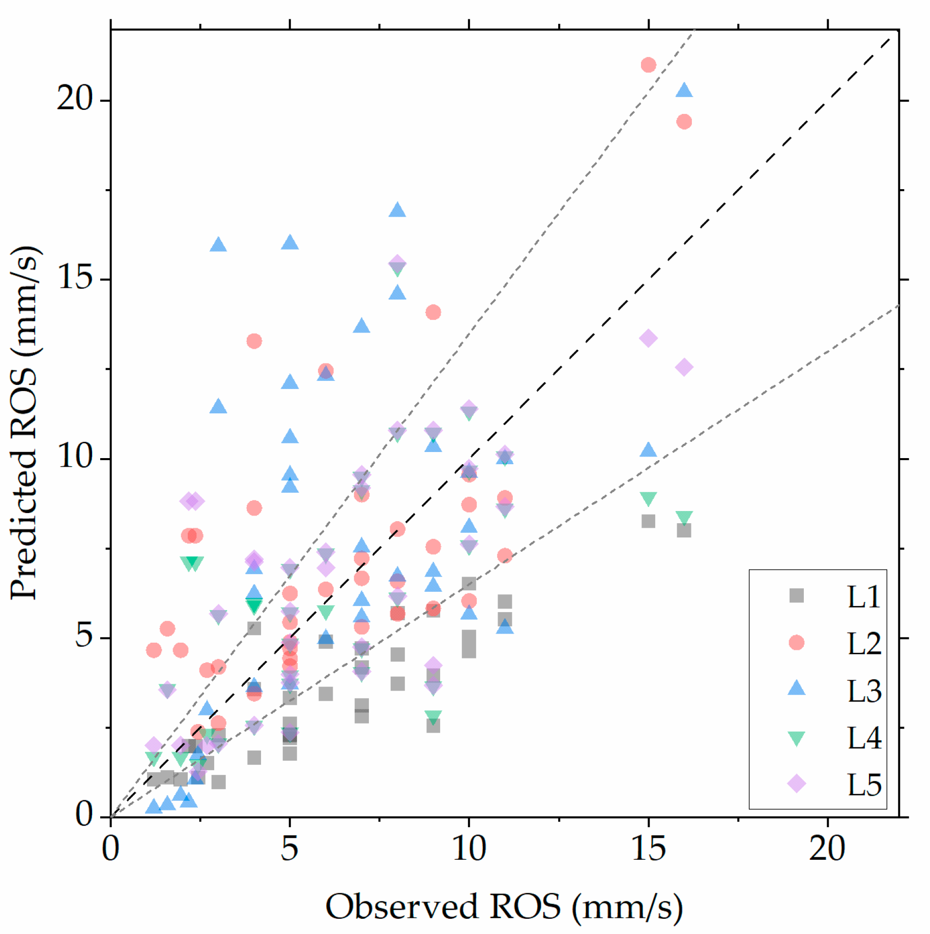
Figure 1. Comparison of measured ROS values for the 37 no-wind tests against predicted ROS values using the five laboratory-developed models.
Fire 06 00188 g001
Figure 2. Relative error of laboratory-developed models as a function of (dry) fuel load for the 37 no-wind fire tests.
Fire 06 00188 g002
Figure 3. Comparison of measured ROS values for the 166 wind tests against predicted ROS values using the two “wind correction” sub-models (W1: left; W2: right), applied to the five laboratory-developed models.
Fire 06 00188 g003
Figure 4. Relative error as a function of wind velocity (top) and packing ratio (bottom) for the ten combinations of laboratory-developed ROS models and wind corrections.
Fire 06 00188 g004
Figure 5. Comparison of measured ROS values for the 166 wind tests against predicted ROS values using the five field-developed models.
Fire 06 00188 g005
Table 1. Name, type, general formula and reference of the selected models.
Model TypeModelGeneral FormRef.
ROS models developed
using
laboratory tests
L1 R 0 = I R , 1 σ , β , h , M , m n , S e ξ 1 σ , β L 1 ( σ , Μ , ρ b ) [10]
L2 R 0 = I R , 2 σ , β , δ , h v , M , m d , Q p , Q w ξ 2 σ , β L 2 ( σ , Μ , ρ b , Q p , Q w ) [11]
L3 R = I P , 3 σ , β , M , U L 2 ( σ , M , ρ b , Q p , Q w ) [12]
L4 R 0 = A 4 M B 4 δ C 4 [13]
L5 R 0 = A 5 M B 5 δ C 5 ln D 5 s [13]
“Wind
correction” sub-models
W1 R = R 0 1 + Φ W , Φ W = A 6 σ , β U B 6 σ [10]
W2 R = f i l R 0 R u , R u = 1 + A 7 U B 7 m ˙ C 7 δ H f 0 D 7 [14]
ROS models developed
using
field tests
F1 R = A 8 U z B 8 F C C 8 M D 8 [15]
F2 R = A 9 U z B 9 δ C 9 e D 9 M 1 + E 9 e F 9 W 2 [16]
F3 R = A 10 U z B 10 ρ b C 10 e D 10 M 1 + E 10 e F 10 W 2 [16]
F4 R = A 11 U z B 11 e C 11 M δ D 11 [17]
F5 R = a ( 1 e b I S I ) c [18]
Table 2. Summary of the experimental studies used for model assessment.
Ref.Fire TestsNo-Wind/Wind TestsFuel Type
[25]92/7Pine needles (Pinus Pinaster)
[26]60/6Bamboo sticks
[27]16330/133Pine needles (Pinus Ponderosa)/Excelsior
[28]71/6Pine needles (Pinus Sibirica)
[29]184/14Pine needles (Pinus Sibirica)
Table 3. Error metric values of the laboratory-developed ROS model predictions for the 37 no-wind fire tests.
ModelRMSEMAPE (%)MBE
L13.542.8−2.8
L23.259.31.0
L34.771.61.5
L43.145.8−0.2
L52.950.90.3
Table 4. Error metric values of predictions using the laboratory-developed ROS models/wind correction combinations for the 166 external wind fire tests.
ModelsRMSEMAPE (%)MBE
L1-W140.146.5−25.3
L2-W151.559.214.8
L3-W191.849.330.8
L4-W140.252.0−6.7
L5-W142.143.11.2
L1-W2143.878.034.4
L2-W2127.8105.335.2
L3-W2101.067.126.8
L4-W2131.394.933.7
L5-W2124.590.133.0
Table 5. Error metric values of the field-developed ROS model predictions for the 166 wind fire tests.
ModelRMSEMAPE (%)MBE
F159.2119.0−24.0
F244.467.5−21.2
F330.763.1−3.9
F451.5231.335.2
F5280.01278.3251.6
Table 6. Absolute and relative change in the RMSE values, resulting from the ±25% relative change in the values of six model parameters.
ParameterModel−25% ChangeAssumed Value+25% Change
hL14.42 (25.9%)3.512.67 (−23.8%)
StL13.46 (−1.5%)3.513.56 (1.5%)
SeL13.31 (−5.6%)3.513.65 (4.2%)
MxL13.80 (8.3%)3.513.31 (−5.7%)
hvL22.82 (−13.0%)3.244.70 (45.3%)
filW2 (L5-W2)85.70 (−31.2%)124.50165.84 (33.2%)
Disclaimer/Publisher’s Note: The statements, opinions and data contained in all publications are solely those of the individual author(s) and contributor(s) and not of MDPI and/or the editor(s). MDPI and/or the editor(s) disclaim responsibility for any injury to people or property resulting from any ideas, methods, instructions or products referred to in the content.