


Time Series Classification with Multiple Wavelength Scattering Signals for Nuisance Alarm Mitigation


Abstract
:1. Introduction
2. Backgrounds
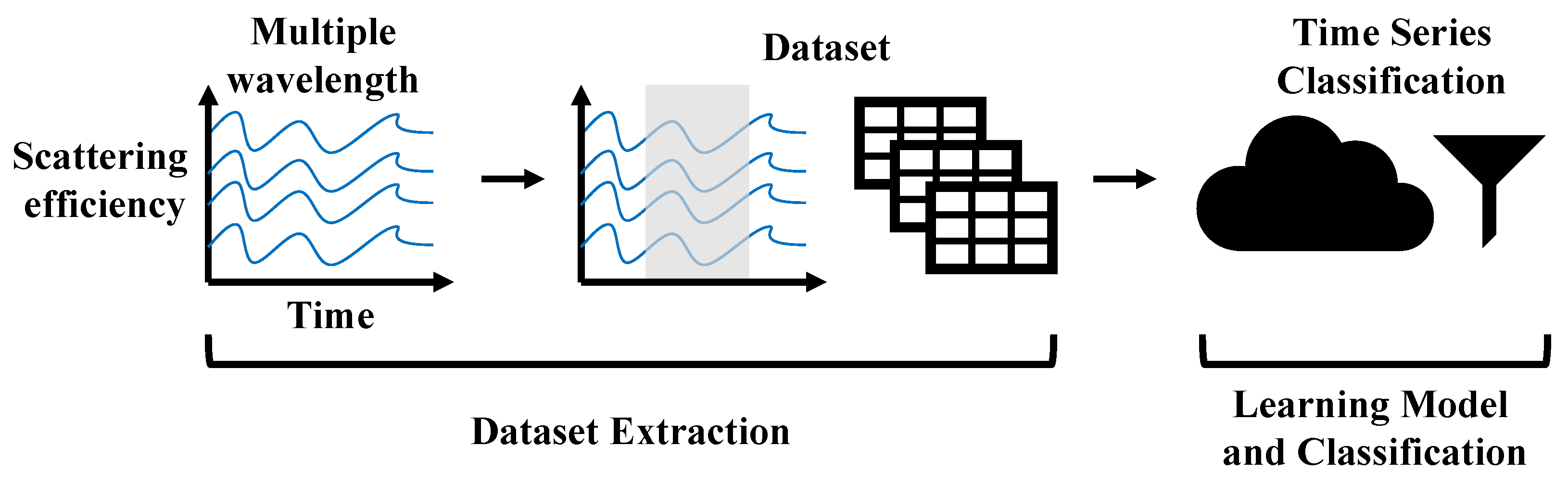
3. Methodology
3.1. Dataset Extraction
3.1.1. Threshold Detection
3.1.2. Two-Sided Cumulative Sum
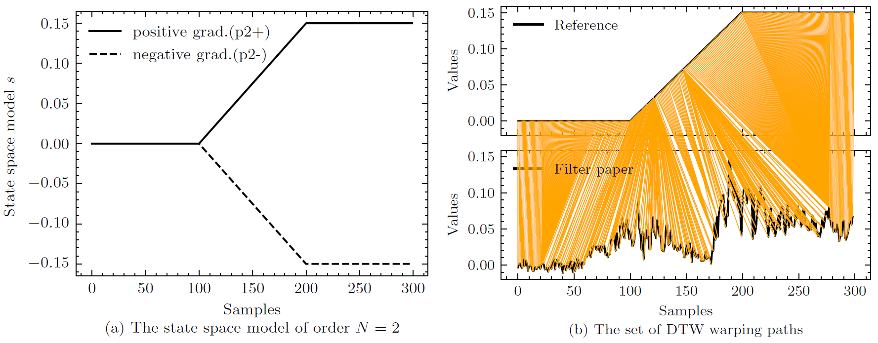
3.1.3. Dynamic Time Warping with Reference Sequences
3.2. Learning Model and Classification
4. Results
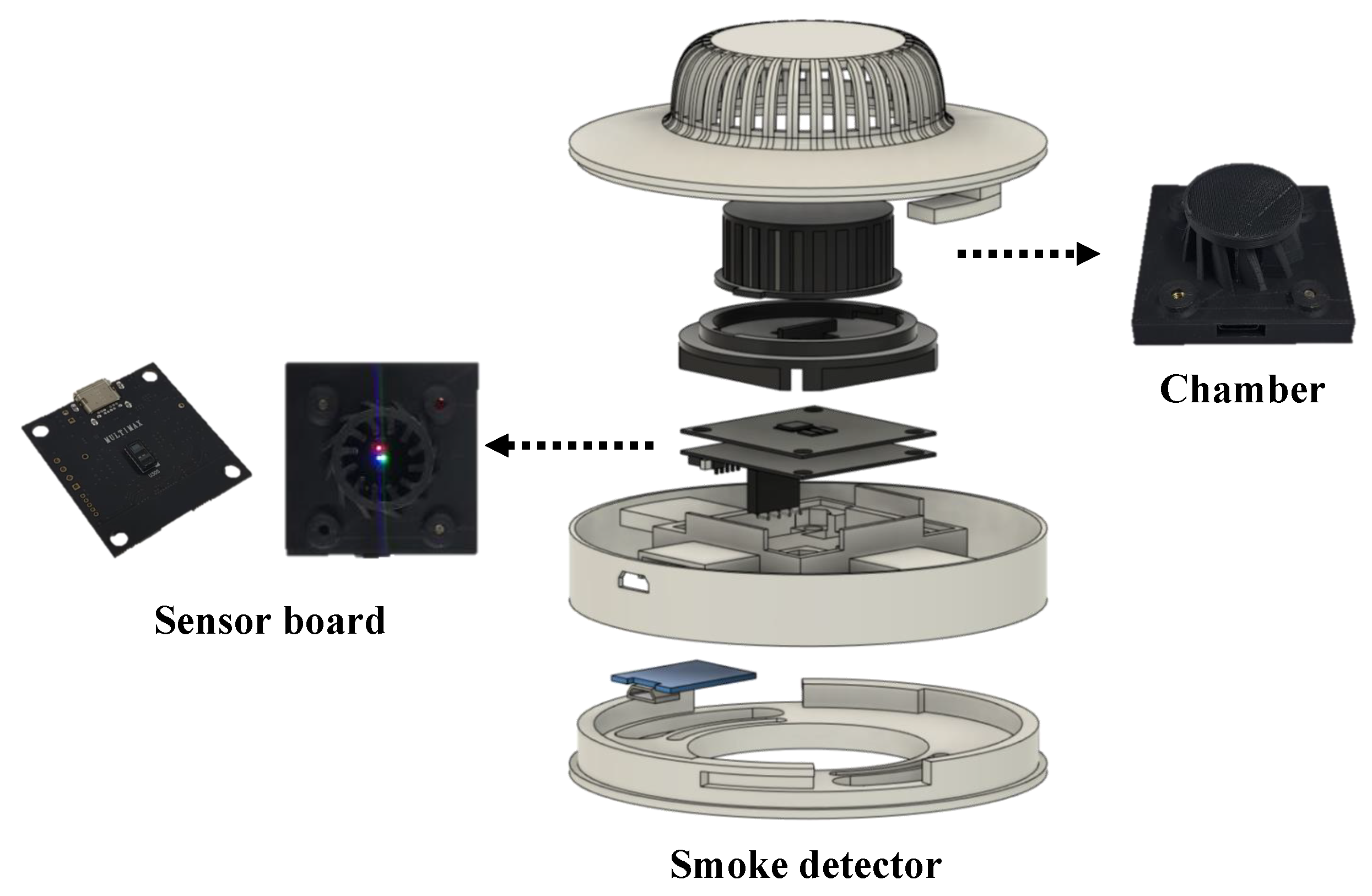
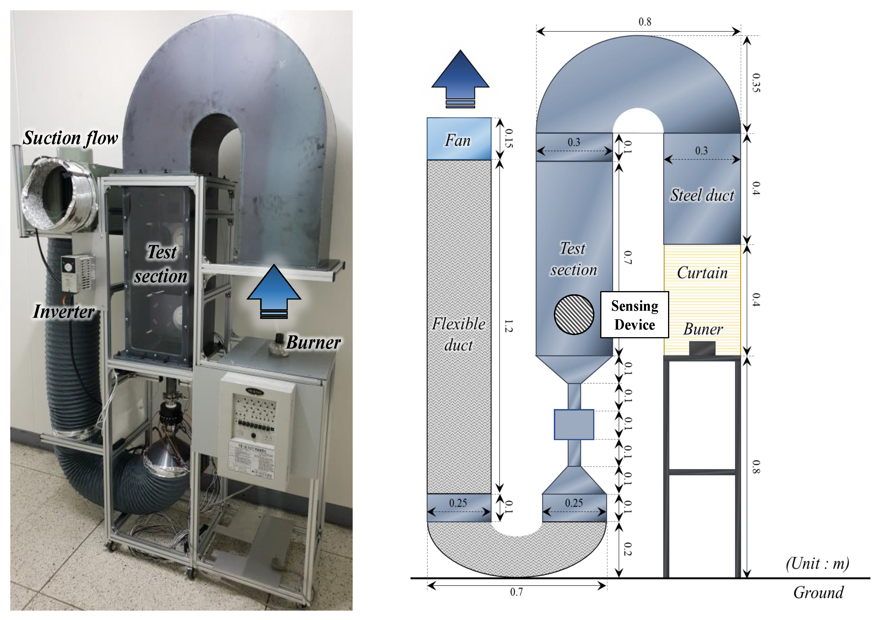
4.1. Design of the Sensing Device and the Experimental Equipment
4.2. Dataset and Learning Models
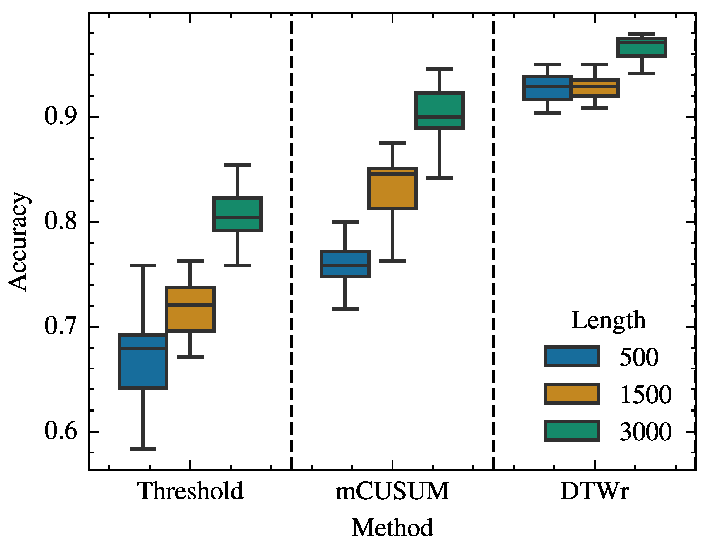
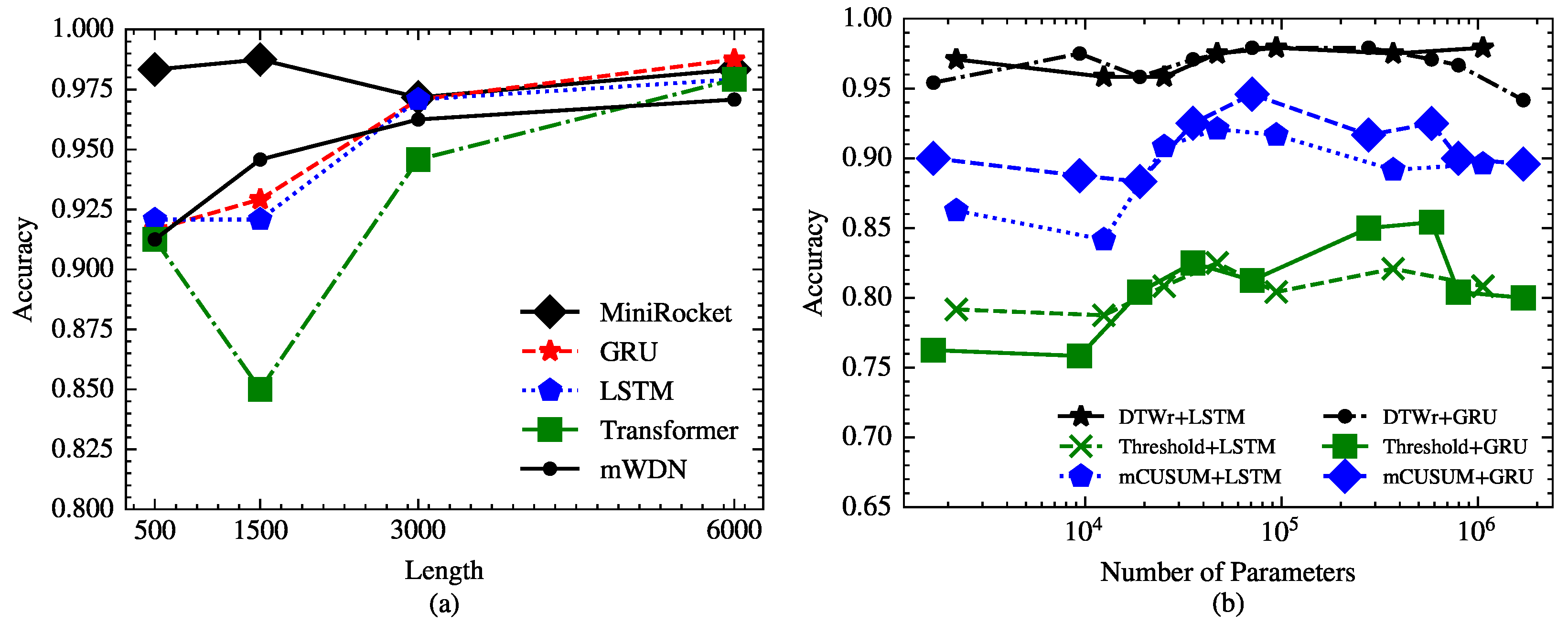
4.3. Performance Comparison
5. Ablation Study
6. Conclusions
Author Contributions
Funding
Institutional Review Board Statement
Informed Consent Statement
Data Availability Statement
Conflicts of Interest
Abbreviations
| UL | Underwriters Laboratories |
| MATLAB | Matrix Laboratory |
| CUSUM | Cumulative Sum |
| DTW | Dynamic Time Warping |
| LSTM | Long Short-Term Memory |
| GRU | Gated Recurrent Unit |
References
- Lee, A.; Pineda, D. Smoke Alarms—Pilot Study of Nuisance Alarms Associated with Cooking; U.S. Consumer Product Safety Commission: Bethesda, MD, USA, 2010; pp. 1–3. [Google Scholar]
- UL 268-2016; UL268: UL Standard for Safety Smoke Detectors for Fire Alarm Systems. 7th ed. UL: Northbrook, IL, USA, 2023; pp. 192–208.
- Yan, S.; Deng, T.; Xu, W.; Wang, S. Selecting an Optimal Set of Scattering Angles and Wavelengths for Practical Photoelectric Smoke Detector. In Proceedings of the 2017 Suppression, Detection, and Signaling Research and Applications Conference, College Park, MD, USA, 12–14 September 2017. [Google Scholar]
- Zhang, Q.; Liu, Z.; Luo, J.; Wang, F.; Wang, J.; Zhang, Y. Characterization of Typical Fire and Non-fire Aerosols by Polarized Light Scattering for Reliable Optical Smoke Detection. In Proceedings of the 11th Asia-Oceania Symposium on Fire Science and Technology, Taipei, Taiwan, 22–24 October 2018; pp. 791–801. [Google Scholar]
- Deng, T.; Wang, S.; Zhu, M. Dual-wavelength optical sensor for measuring the surface area concentration and the volume concentration of aerosols. Sens. Actuators B Chem. 2016, 236, 334–342. [Google Scholar] [CrossRef]
- Krüll, W.; Schultze, T.; Tobera, R.; Willms, I. Characterization of Dust and Water Steam Aerosols in False Alarm Scenarios—Design of a Test Method for Fire Detectors in Dusty and in Highly Foggy Environments. In Proceedings of the 2015 Suppression, Detection, and Signaling Research and Applications Conference, Orlando, FL, USA, 3 March 2015. [Google Scholar]
- Li, K.; Liu, G.; Yuan, H.; Chen, Y.; Dai, Y.; Meng, X.; Kang, Y.; Huang, L. Dual-Wavelength Smoke Detector Measuring Both Light Scattering and Extinction to Reduce False Alarms. Fire 2023, 6, 140. [Google Scholar] [CrossRef]
- Wegrzyriski, W.; Antosiewiez, P.; Fangrat, J. Multi-Wavelength Densitometer for Experimental Research on the Optical Characteristics of Smoke Layers. Fire Technol. 2021, 57, 2683–2706. [Google Scholar] [CrossRef]
- Van de Hulst, H.C. Light Scattering by Small Particles. Q. J. R. Meteorol. Soc. 1957, 84, 198–199. [Google Scholar] [CrossRef]
- Christian, M. MATLAB Functions for Mie Scattering and Absorption; Institut für Angewandte Physik: Bern, Switzerland, 2002. [Google Scholar]
- Cole, M. Aerosol characterisation for reliable ASD operation. In Proceedings of the 14th International Conference on Automatic Fire Detection, Duisburg, Germany, 8–10 September 2009. [Google Scholar]
- Han, K.; Kim, S.; Yang, H.; Cho, K.S.; Lee, K.; Han, H. Statistical Characteristics of Scattering Ratio Based on Three Optical Wavelengths for Smoke Particles. Int. J. Fire Sci. Eng. 2022, 36, 40–49. [Google Scholar] [CrossRef]
- Ahn, Y.; Han, K.; Yang, H.; Kim, S.; Ryu, J.; Lee, K. Smoke Particle-Source Prediction Model Based on Multiple Optical Wavelengths Using Deep Learning. Int. J. Fire Sci. Eng. 2023, 37, 20–29. [Google Scholar] [CrossRef]
- TPS8802 Smoke Alarm AFE. Available online: https://www.ti.com/document-viewer/tps8802/datasheet (accessed on 13 November 2023).
- Integrated Optical Module for Smoke Detection. Available online: https://www.analog.com/media/en/technical-documentation/data-sheets/adpd188bi.pdf (accessed on 13 November 2023).
- Smoke Testing with the ADPD188BI Optical Smoke and Aerosol Detection Module. Available online: https://www.analog.com/media/en/technical-documentation/app-notes/an-1567.pdf (accessed on 13 November 2023).
- Ren, E.; Zalmai, N.; Loeliger, H. Multi-channel Information Processing for Fire Detection. In Proceedings of the 2017 Suppression, Detection, and Signaling Research and Applications Conference, Hyattsville, MD, USA, 12 September 2017. [Google Scholar]
- Geiman, J.; Gottuk, D.T. Alarm Thresholds for Smoke Detector Modeling. In Fire Safety Science, Proceedings of the Seventh International Symposium, Worcester, MA, USA, 16–21 June 2002; pp. 197–208. [Google Scholar]
- Granjon, P. The CuSum Algorithm—A Small Review. 2013. ID: hal-00914697f. Available online: https://hal.science/hal-00914697 (accessed on 26 December 2023).
- Wildhaber, R.A.; Zalmai, N.; Jacomet, M.; Loeliger, H. Windowed State-Space Filters for Signal Detection and Separation. IEEE Trans. Signal Process. 2018, 66, 3768–3783. [Google Scholar] [CrossRef]
- Keogh, E.; Ratanamahatana, C.A. Exact indexing of dynamic time warping. Knowl. Inf. Syst. 2005, 7, 357–386. [Google Scholar] [CrossRef]
- Giorgino, T. Computing and Visualizing Dynamic Time Warping Alignments in R: The dtw Package. J. Stat. Softw. 2009, 31, 1–24. [Google Scholar] [CrossRef]
- Hochreiter, S.; Schmidhuber, J. Long short-term memory. Neural Comput. 1997, 9, 1735–1780. [Google Scholar] [CrossRef] [PubMed]
- Chung, J.; Gulcehre, C.; Cho, K.; Bengio, Y. Empirical Evaluation of Gated Recurrent Neural Networks on Sequence Modeling. In Proceedings of the NIPS 2014 Deep Learning and Representation Learning Workshop, Montréal, QC, Canada, 8 December 2014. [Google Scholar]
- Wang, J.; Wang, Z.; Li, J.; Wu, J. Multilevel Wavelet Decomposition Network for Interpretable Time Series Analysis. In Proceedings of the KDD ’18: 24th ACM SIGKDD International Conference on Knowledge Discovery & Data Mining, London, UK, 19 August 2018; pp. 2437–2446. [Google Scholar]
- Vaswani, A.; Shazeer, N.; Parmar, N.; Uszkoreit, J.; Jones, L.; Gomez, A.N.; Kaiser, L.; Polosukhin, I. Transformer: Attention is All You Need. In Proceedings of the 31st Conference on Neural Information Processing Systems (NIPS 2017), Long Beach, CA, USA, 4–9 December 2017. [Google Scholar]
- Dempster, A.; Petitjean, F.; Webb, G.I. ROCKET: Exceptionally fast and accurate time series classification using random convolutional kernels. Data Min. Knowl. Discov. 2020, 34, 1454–1495. [Google Scholar] [CrossRef]
- Dempster, A.; Schmidt, D.F.; Webb, G.I. MiniRocket: A Very Fast (Almost) Deterministic Transform for Time Series Classification. In Proceedings of the KDD ’21: 27th ACM SIGKDD Conference on Knowledge Discovery & Data Mining, New York, NY, USA, 14 August 2021. [Google Scholar]
- Integrated Optical Sensor Module for Mobile Health. Available online: https://www.analog.com/media/en/technical-documentation/data-sheets/max86916.pdf (accessed on 13 November 2023).
- Jang, H.; Hwang, C. Preliminary Study for Smoke Color Classification of Combustibles Using the Distribution of Light Scattering by Smoke Particles. Appl. Sci. 2023, 13, 669. [Google Scholar] [CrossRef]
- tsai—A State-of-the-Art Deep Learning Library for Time Series and Sequential Data. Available online: https://github.com/timeseriesAI/tsai (accessed on 13 November 2023).
- Kharitonov, E.; Chaabouni, R. What they do when in doubt: A study of inductive biases in seq2seq learners. In Proceedings of the ICLR 2021, Vienna, Austria, 4 May 2021. [Google Scholar]


| Label | Source |
|---|---|
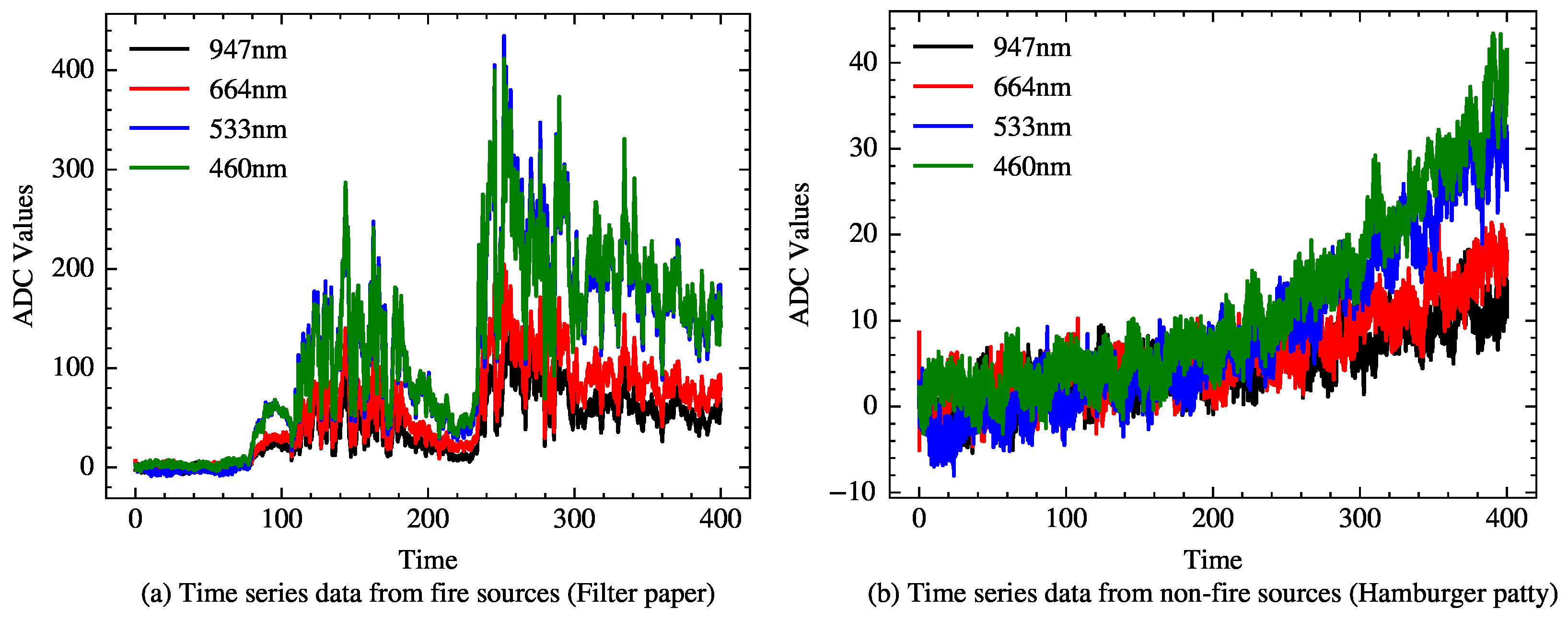
| Test #01∼Test #20 | Filter paper |
| Test #21∼Test #40 | Kerosene |
| Test #41∼Test #60 | Polyethylene |
| Test #61∼Test #80 | Dust |
| Test #81∼Test #100 | Hamburger patty |
| Test #101∼Test #120 | Vapor |
| Feature 1 | The difference between the ADC values and the mean of the initial idle ADC values at 947 nm wavelength |
| Feature 2 | The difference between the ADC values and the mean of the initial idle ADC values at 664 nm wavelength |
| Feature 3 | The difference between the ADC values and the mean of the initial idle ADC values at 533 nm wavelength |
| Feature 4 | The difference between the ADC values and the mean of the initial idle ADC values at 460 nm wavelength |
| Feature 5 | The ratio of the ADC values to the mean of the initial idle ADC values at 947 nm wavelength |
| Feature 6 | The ratio of the ADC values to the mean of the initial idle ADC values at 664 nm wavelength |
| Feature 7 | The ratio of the ADC values to the mean of the initial idle ADC values at 533 nm wavelength |
| Feature 8 | The ratio of the ADC values to the mean of the initial idle ADC values at 460 nm wavelength |
| Methodology | Threshold-based method (Threshold) Multivariate CUSUM-based method (mCUSUM) DTW-based method with reference sequences (DTWr) | |
| Length | 500/1500/3000 | |
| Models | TransformerModel | {} |
| mWDN | {’levels’: 4} | |
| MiniRocket | {} | |
| GRU | {’n_layers’: 1/5/10, ’bidirectional’: True/False, ’hidden_size’: 10/100} | |
| LSTM | {’n_layers’: 1/5/10, ’bidirectional’: True/False, ’hidden_size’: 10/100} |
| Length | No. | Method | ||||||||
|---|---|---|---|---|---|---|---|---|---|---|
| Threshold | mCUSUM | DTWr | ||||||||
| Arch. Hyperparams. | Accuracy | F1 Score | Arch. Hyperparams. | Accuracy | F1 Score | Arch. Hyperparams. | Accuracy | F1 Score | ||
| 500 | 1 | MiniRocket {} | 0.7583 | 0.7576 | MiniRocket {} | 0.9167 | 0.9164 | MiniRocket {} | 0.9833 | 0.9833 |
| 2 | GRU {’n_layers’: 5, ’bidirectional’: True, ’hidden_size’: 100} | 0.7125 | 0.7120 | TransformerModel {} | 0.8000 | 0.8014 | GRU {’n_layers’: 5, ’bidirectional’: True, ’hidden_size’: 100} | 0.9450 | 0.9495 | |
| 3 | GRU {’n_layers’: 10, ’bidirectional’: True, ’hidden_size’: 100} | 0.7042 | 0.7043 | GRU {’n_layers’: 1, ’bidirectional’: True, ’hidden_size’: 10} | 0.7958 | 0.7910 | LSTM {’n_layers’: 5, ’bidirectional’: False, ’hidden_size’: 100} | 0.9458 | 0.9451 | |
| 4 | GRU {’n_layers’: 10, ’bidirectional’: False, ’hidden_size’: 100} | 0.7041 | 0.7042 | GRU {’n_layers’: 5, ’bidirectional’: True, ’hidden_size’: 10} | 0.7792 | 0.7778 | LSTM {’n_layers’: 5, ’bidirectional’: True, ’hidden_size’: 100} | 0.9417 | 0.9410 | |
| 5 | GRU {’n_layers’: 5, ’bidirectional’: False, ’hidden_size’: 100} | 0.6958 | 0.6965 | GRU {’n_layers’: 10, ’bidirectional’: True, ’hidden_size’: 100} | 0.7750 | 0.7703 | GRU {’n_layers’: 1, ’bidirectional’: True, ’hidden_size’: 100} | 0.9417 | 0.9409 | |
| 1500 | 1 | MiniRocket {} | 0.8458 | 0.8455 | MiniRocket {} | 0.9208 | 0.9201 | MiniRocket {} | 0.9875 | 0.9875 |
| 2 | GRU {’n_layers’: 1, ’bidirectional’: False, ’hidden_size’: 100} | 0.7625 | 0.7629 | LSTM {’n_layers’: 5, ’bidirectional’: True, ’hidden_size’: 10} | 0.8750 | 0.8715 | LSTM {’n_layers’: 1, ’bidirectional’: False, ’hidden_size’: 100} | 0.9500 | 0.9492 | |
| 3 | TransformerModel {} | 0.7500 | 0.7464 | LSTM {’n_layers’: 1, ’bidirectional’: True, ’hidden_size’: 100} | 0.8708 | 0.8656 | mWDN {’levels’: 4} | 0.9458 | 0.9450 | |
| 4 | GRU {’n_layers’: 1, ’bidirectional’: True, ’hidden_size’: 100} | 0.7458 | 0.7461 | GRU {’n_layers’: 1, ’bidirectional’: True, ’hidden_size’: 100} | 0.8625 | 0.8582 | LSTM {’n_layers’: 1, ’bidirectional’: True, ’hidden_size’: 10} | 0.9417 | 0.9410 | |
| 5 | GRU {’n_layers’: 10, ’bidirectional’: True, ’hidden_size’: 100} | 0.7417 | 0.7427 | TransformerModel {} | 0.8542 | 0.8532 | GRU {’n_layers’: 1, ’bidirectional’: True, ’hidden_size’: 100} | 0.9417 | 0.9410 | |
| 3000 | 1 | MiniRocket {} | 0.9125 | 0.9090 | GRU {’n_layers’: 1, ’bidirectional’: True, ’hidden_size’: 100} | 0.9458 | 0.9455 | GRU {’n_layers’: 5, ’bidirectional’: False, ’hidden_size’: 100} | 0.9792 | 0.9791 |
| 2 | GRU {’n_layers’: 10, ’bidirectional’: False, ’hidden_size’: 100} | 0.8542 | 0.8531 | MiniRocket {} | 0.9375 | 0.9334 | LSTM {’n_layers’: 1, ’bidirectional’: True, ’hidden_size’: 100} | 0.9717 | 0.9791 | |
| 3 | GRU {’n_layers’: 5, ’bidirectional’: False, ’hidden_size’: 100} | 0.9500 | 0.8489 | mWDN {’levels’: 4} | 0.9333 | 0.9330 | LSTM {’n_layers’: 5, ’bidirectional’: True, ’hidden_size’: 100} | 0.9792 | 0.9790 | |
| 4 | LSTM {’n_layers’: 1, ’bidirectional’: False, ’hidden_size’: 100} | 0.8250 | 0.8229 | GRU {’n_layers’: 10, ’bidirectional’: False, ’hidden_size’: 100} | 0.9250 | 0.9239 | GRU {’n_layers’: 1, ’bidirectional’: True, ’hidden_size’: 100} | 0.9792 | 0.9790 | |
| 5 | GRU {’n_layers’: 1, ’bidirectional’: False, ’hidden_size’: 100} | 0.8250 | 0.8225 | GRU {’n_layers’: 1, ’bidirectional’: False, ’hidden_size’: 100} | 0.9250 | 0.9239 | LSTM {’n_layers’: 5, ’bidirectional’: False, ’hidden_size’: 100} | 0.9750 | 0.9750 | |
Disclaimer/Publisher’s Note: The statements, opinions and data contained in all publications are solely those of the individual author(s) and contributor(s) and not of MDPI and/or the editor(s). MDPI and/or the editor(s) disclaim responsibility for any injury to people or property resulting from any ideas, methods, instructions or products referred to in the content. |
© 2023 by the authors. Licensee MDPI, Basel, Switzerland. This article is an open access article distributed under the terms and conditions of the Creative Commons Attribution (CC BY) license (https://creativecommons.org/licenses/by/4.0/).
Share and Cite
Han, K.; Kim, S.; Yang, H.; Cho, K.; Lee, K. Time Series Classification with Multiple Wavelength Scattering Signals for Nuisance Alarm Mitigation. Fire 2024, 7, 14. https://doi.org/10.3390/fire7010014
Han K, Kim S, Yang H, Cho K, Lee K. Time Series Classification with Multiple Wavelength Scattering Signals for Nuisance Alarm Mitigation. Fire. 2024; 7(1):14. https://doi.org/10.3390/fire7010014
Chicago/Turabian StyleHan, Kyuwon, Soocheol Kim, Hoesung Yang, Kwangsoo Cho, and Kangbok Lee. 2024. "Time Series Classification with Multiple Wavelength Scattering Signals for Nuisance Alarm Mitigation" Fire 7, no. 1: 14. https://doi.org/10.3390/fire7010014
APA StyleHan, K., Kim, S., Yang, H., Cho, K., & Lee, K. (2024). Time Series Classification with Multiple Wavelength Scattering Signals for Nuisance Alarm Mitigation. Fire, 7(1), 14. https://doi.org/10.3390/fire7010014