Remote Sensing Active Fire Detection Tools Support Growth Reconstruction for Large Boreal Wildfires

Abstract

Spatial and temporal estimates of burned areas are often used to model greenhouse gas and air pollutant emissions from fire events that occur in a region of interest and over specified time frames. However, fire behaviour, fuel consumption, fire severity, and ecological effects vary over both time and space when a fire grows across varying fuels and topography under different environmental conditions. We developed a method for estimating the progression of individual wildfires (i.e., day-of-burn) employing ordinary kriging of a combination of different satellite-based active fire detection data sources. We compared kriging results obtained using active fire detection products from the Moderate Resolution Imaging Spectroradiometer (MODIS), the Visible Infrared Imaging Radiometer Suite (VIIRS), and combined MODIS and VIIRS data to study how inferences about a wildfire’s evolution vary among data sources. A quasi-validation procedure using combined MODIS and VIIRS active fire detection products that we applied to an independent data set of 37 wildfires that occurred in the boreal forest region of the province of Ontario, Canada, resulted in nearly half of each fire’s burned area being accurately estimated to within one day of when it actually burned. Our results demonstrate the strengths and limitations of this geospatial interpolation approach to mapping the progression of individual wildfires in the boreal forest region of Canada. Our study findings highlight the need for future validations to account for the presence of spatial autocorrelation, a pervasive issue in ecology that is often neglected in day-of-burn analyses.

1. Introduction

Estimates of the area burned by wildfires are used to model carbon, gas, and aerosol emissions and are the basis for assessing the effects of fire regimes on the atmosphere and biogeochemical cycles [1,2,3]. The burning of vegetative biomass affects terrestrial environments by altering their structure, function, and species composition, consequently affecting ecosystem services, biodiversity, and economic, social, and cultural values [4]. Although it is not feasible, due to financial and logistical constraints, to conduct comprehensive, ground-based documentation of every fire’s evolution across large geographic regions, satellite-based active fire and burn scar imagery can be employed to monitor some burned area attributes at regional and global scales [5,6,7,8]. For example, national and international fire management organizations have compiled publicly available fire imagery to monitor fires for decades (Canadian Wildland Fire Information System [9], European Forest Fire Information System [10], and Global Wildfire Information System [11].

Satellite-based thermal infrared sensors are used for the global detection of actively burning vegetation fires based on observations of radiant emissions from the middle infrared (3–5 µm) and the longwave infrared (8–12 µm) spectral regions [12]. Dozier (1981) found that subpixel-sized fires could be identified using thermal infrared sensor observations having a moderate spatial resolution (1 km²) [13]. Active fire detection algorithms were developed and applied to such spectral radiance data to discriminate biomass burning and record it as a time series of spatial point data, colloquially known as “hotspots” [14,15,16,17]. The term “actively burning” suggests that there is a minimum detectable fire size and temperature implicit in the fire detection algorithm, and thus the temperature of smouldering fires (i.e., “passively” or “inactively” burning fires) may not meet the threshold criteria [18]. The minimum detectable fire temperature (and fire radiative power) scales with the sensor’s ground pixel area (ground sampling distance) [19]. Active fire detection data have been acquired using the Advanced Very-High-Resolution Radiometer (AVHRR [20]), the Advanced Thermal Scanning Radiometer (ATSR [21]), the Moderate Resolution Imaging Spectroradiometer Suite (MODIS [22]), and the Visible Infrared Imaging Radiometer Suite (VIIRS [23,24]).

Expanding on classical approaches for studying fire regimes (e.g., fire history maps, tree cores, and charcoal records [25,26,27]), researchers are exploring methods that rely on active fire and burned area products to characterize spatial and temporal variability in fire activity. Early work with satellite active fire products examined the detection rates (i.e., fire counts) of the ATSR sensor relative to area burned maps and annual area burned statistics for Canada and Alaska [28]. Another study estimated fire spread by grouping individual MODIS hotspots into separate clusters representing wildfire events using a spatial-temporal filter and measuring the distances between hotspots acquired from consecutive satellite overpasses to produce estimates of spread rate (in km/h) for fires that occurred in northern Eurasia [29]. Their chosen clustering algorithm, the density-based spatial clustering of applications with noise, is a data mining approach that, in their application, identifies individual (often multiday) fire events, thereby circumventing the need for final burned area maps to assign hotspots to a single fire event in data processing [30]. Day-of-burn maps that reconstruct the progression of a spreading wildfire at coarse spatio-temporal scales (i.e., >1 km² and daily) have been based primarily on the input of active fire detections and a burn mask [31,32,33,34,35]. Another approach to burn date mapping, the MODIS MCD64A1 product, is a combination of burned area and active fire detections used to estimate the burn date for 500 m × 500 m grid cells [36]. As part of the Artic Boreal Vulnerability Experiment, a historical atlas of interpolated burn dates within fire scars was generated using MODIS and VIIRS hotspots for large fires that occurred in Canada and Alaska [37]. MODIS and VIIRS hotspots were also used to predict continuous fire progression maps at a daily time interval for fires in Northern California [38]. Bayesian Updating of Land Cover has been used to generate fire progression maps from a composite burned area mapping time series [39]. Deep learning frameworks have been developed to monitor a fire’s progression using Synthetic Aperture Radar [40]. Reducing the uncertainty associated with burn date estimates was the focus of a study in which Synthetic Aperture Radar imagery was used to reduce error in the pixel-based estimates of the burn date of the MODIS MCD64A1 product, thereby increasing the quality and confidence of the overall mapping product [41].

Many research questions pertaining to the analysis of historical wildfire growth hinge on knowing the day on which different parts of a large fire burned, primarily to explain or predict specific aspects of fire effects (

Table 1. Selected fire behaviour and effect research questions that have been explored using satellite-based fire reconstruction maps.

Research Question	Statistical Approach	Data Sources	Findings
Do weather, topography, vegetation type, and time since last fire affect fire severity? [46]	Regression tree analysis (n = 2 fires)	Landsat	Higher relative humidity, lower temperatures, and a shorter time since the last fire corresponded with low and moderate fire severity. Lodgepole pine stands burning at low wind speeds often had higher mortality rates.
Do weather and time since last fire constrain subsequent fire spread? [47]	Categorical tree analysis, logistic regression analysis (n = 19 fires)	Landsat	Low to moderate fire weather and time since fire less than 9 years constrained spread; evidence that fire is “self-limiting”.
Characterize the relative importance of weather, topography, and previous burns on crown damage. [48]	Regression tree analysis, random forest (n = 1 fire)	Digital aerial photography	The air temperature and burn period (in weeks instead of days) were associated with high crown damage.
Is daily area burned correlated with burn severity? [49]	Correlation (n = 42 fires)	Landsat, airborne thermal infrared scans	The proportion of high burn severity was weakly correlated with the size of the daily burned area.
How do Santa Ana wind events affect daily area burned? [50]	Kolmogorov–Smirnov test, t-test, generalized linear model (n = 158 fires)	Landsat, MODIS	Increased wind speed and relative humidity associated with Santa Ana winds were significant predictors of burned area per day. The length of the previous day’s burn perimeter was also a significant predictor.
How do potential and realized spread vary across Canada? [51]	Frequency distribution, transformation function, correlation (n = 2246 fires)	MODIS	The ratio of days with fire-conducive weather (Fire Weather Index ≥ 19) to days where actual fire growth was observed varied by region and by latitude.
Do previous burns and weather influence subsequent fire spread? [52]	Logistic regression (n = 1038 fires)	Landsat	Fire progression is controlled by previous fires (i.e., lack of flammable fuels) and weather— evidence that fire is “self-limiting”.
Characterize the relative importance of top-down (daily fire weather) and bottom-up (topography and vegetation) controls on burn severity. [53]	Multivariable generalized linear regression (n = 6 fires)	Landsat	“Prognostic models indicated burn severity was explained by pre-fire stand structure and composition, topo-edaphic context, and fire weather at time of burning”.

). However, a fundamental problem in fire growth reconstruction is that the progress of most wildfires cannot readily be observed continuously. Instead, the timing of their arrival at different locations is estimated (with some accompanying measurement uncertainty). Burn date maps, or alternatively, day-of-burn maps, have been used to (1) compute spatial estimates of the daily area burned and the daily perimeter of a spreading wildfire over many days of growth and (2) evaluate hypothesized relationships between daily fire growth and explanatory variables that may differ over time and space (e.g., fuels, weather, and topography). More recently, the spatial and temporal components of a developing wildfire, including its apparent speed and duration, have been estimated from remotely sensed fire products with the goal of comparing fire regime-related attributes among biomes or ecoregions [42,43,44,45].

Fire progression maps (acquired visually and sketched by personnel aboard an aircraft or via an aircraft-mounted infrared scanner) are seldom collected in remote locations of the boreal forest [54]. In lieu of such agency-recorded maps, satellite-based active fire detections are often used to infer fire progression. However, there are some well-known limitations of active fire products with respect to wildfire mapping. For example, sky conditions (e.g., the presence of clouds) and satellite overpass timing relative to an individual wildfire’s growth will determine if a biomass burning event is detected with the sensor [12]. Neither MODIS nor VIIRS operate over Canadian boreal locations during the time of peak burn at about 16:00 h local standard time or 17:00 h daylight saving time [55], ultimately limiting its use for inferences about peak fire activity and fire behaviour. Since the performance of infrared thermal detection systems varies across the globe [10,22,24], the validation results of day-of-burn maps from other fire-prone regions may not be directly transferable to the Canadian boreal forest region. A better understanding is needed of how well such geospatial interpolation methods perform at Canadian boreal latitudes. To the best of our knowledge, no thorough validation of day-of-burn mapping has been done using Canadian fire perimeters to date.

The objectives of this study were as follows:

(1)

Develop a method to estimate the day of burn for portions of individual wildfires by combining different sources of active fire detection data and using ordinary kriging.

(2)

Use operational burned area update data recorded by Ontario’s Ministry of Natural Resources and Forestry fire operations personnel to validate kriging results.

(3)

Compare results obtained via kriging of MODIS, VIIRS, and combined data to better understand how progression inference varies by data source and kriging method.

2. Materials and Methods

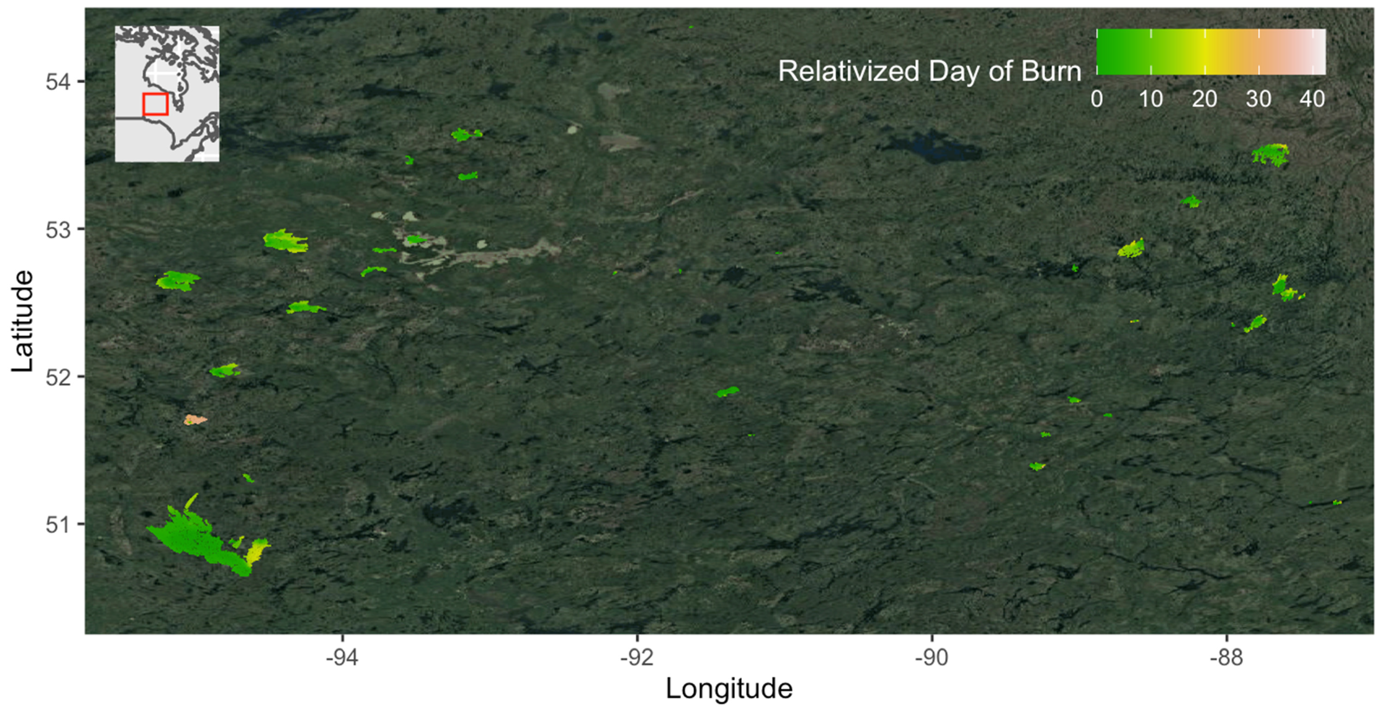
2.1. Wildfire Data

We estimated the progression of 37 wildland fires that occurred in the province of Ontario, Canada. These fires were selected based on available burned area update maps created by the Ontario Ministry of Natural Resources and Forestry’s Aviation, Forest Fire and Emergency Services Branch operations personnel (MNRF AFFES). To be included in the study data set, a fire had to have at least two burned area update maps prepared by AFFES personnel during its growth. In rare cases, different burned area update maps were obtained on the same day, and for our analysis, we used the map from the latest time of day to represent the burned area extent. We confirmed that each final burned area map obtained by MNRF matched the fire polygon recorded in the National Burned Area Composite [56]. The suppression status label assigned to each fire by AFFES indicated that all but one of the fires we studied were ‘Monitored’, meaning they received no significant suppression action; the exception was the fire RED-003-2016, which was categorized as having received ‘Full Suppression’. The 36 monitored fires constitute a novel data set for future study in that they received no human intervention, so inferences about day-to-day growth are not confounded by suppression activities that may have generated anthropogenic thermal signals (e.g., backfiring/burning out operations) or influenced fireline intensity and thus detectability (e.g., use of airtankers and other suppression resources). However, since this study is primarily focused on the accuracy of burn date predictions, we chose to include the validation results for the suppressed fire in our summary statistics. Data were processed, analyzed, and graphed using R statistical software version 4.3.0 [57].

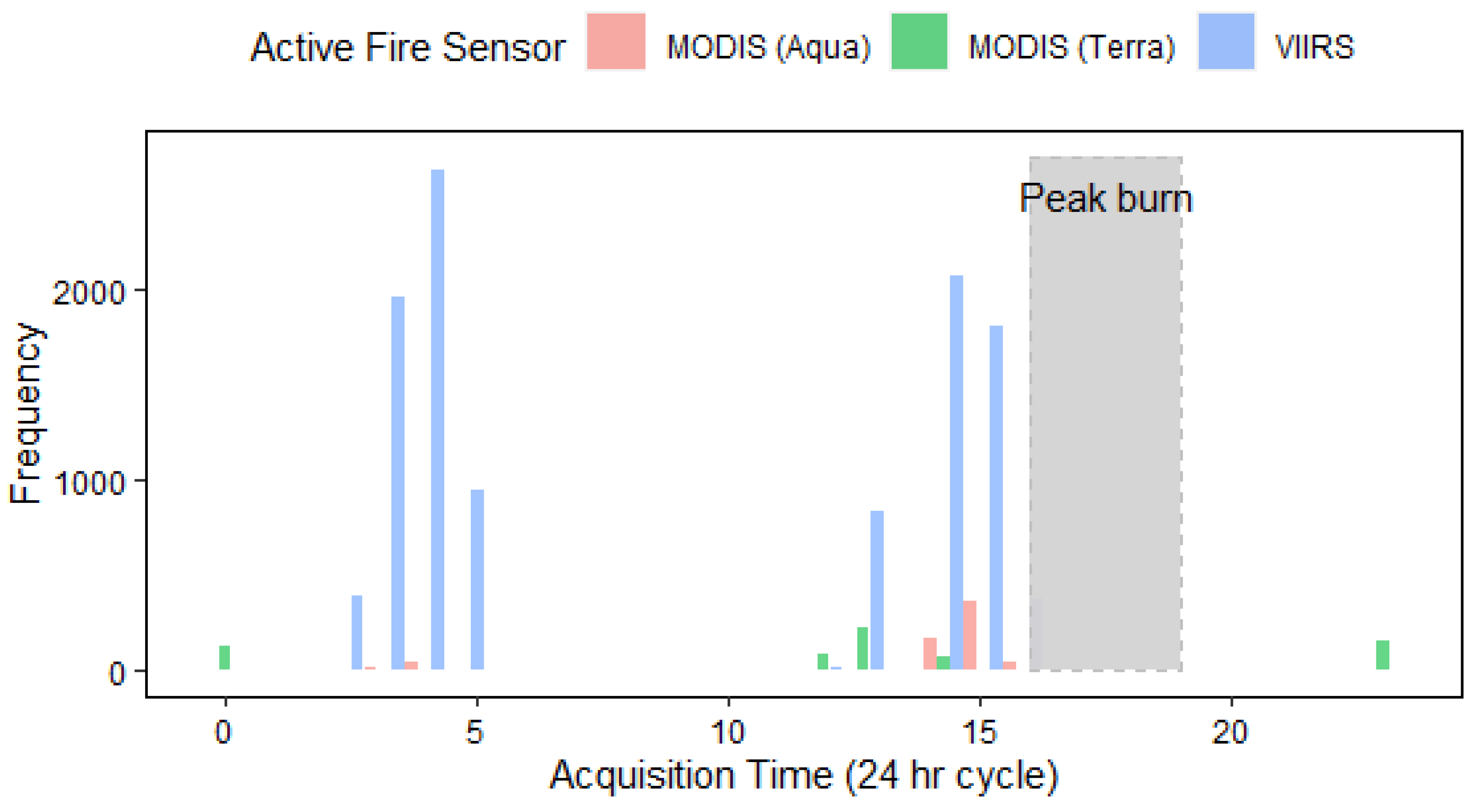
2.2. Active Fire Detection Data

MODIS instruments have been flown on the polar-orbiting Terra and Aqua satellites since 2000 and 2002, respectively. MODIS has 36 channels, a 2000 km swath width, and pixel resolution ranging between 250 m and 1 km (depending on the channel) at nadir. The VIIRS instrument has been flown on the polar-orbiting Suomi NPP satellite since 2011. VIIRS has 22 channels, a 3000 km swath width, and pixel resolution ranging between 375 m (I-bands) and 750 m (M-bands) at nadir. The MODIS and VIIRS thermal anomaly/active fire products contain ‘hotspot’ or ‘fire-pixel’ data based on contextual active fire detection algorithms that exploit a fire’s strong emissions in the mid-infrared spectral region [24,36]. MODIS and VIIRS detect actively flaming and smouldering portions of fires that are 1000 m², although flaming fires of 50 m² have been detected under rare conditions [58]. Active fire detection data from MODIS (1 km pixels, MOD14/MYD14, Collection 6) and VIIRS (375 m pixels, Suomi NPP) were obtained from the US Forest Service Fire Information for Resource Management System [59]. The active fire detection data contain attributes of detection time, location, confidence, and fire radiative power.

For each of the 37 mapped fires, we extracted the MODIS and VIIRS active fire detections in a 1 km buffer around the perimeter of the NBAC fire polygons [60,61], using the “gBuffer” and “gIntersection” functions from the rgeos [62] R package. The fire detections were extracted for the same temporal extents as each fire event, and the buffer was used to ensure that an active fire detection whose centre lies outside of the fire perimeter is included in the extraction. The confidence value (an attribute included in the downloaded data set) is a percentage value assigned to each active fire detection based on intermediate algorithm quantities used in the contextual active fire detection process and is an indication of individual detection quality [63]. For our analysis, an individual hotspot was omitted if its confidence value was less than 40% to remove observations that are potential false alarms while retaining detections associated with a saturated pixel that is free of possible sun glint and contains relative temperature anomaly values >15 degrees Kelvin higher than the background temperature [36]. Although our analysis omitted active fire detections with a confidence value <40%, further data screening could be based specifically on scan angle (view zenith angle) to remove detections near the swath edge. Following the data extraction and screening, we used the time that a fire detection indicated a pixel burned as the input to reconstruct individual fire progressions.

Active fire detections from satellite sensors show instantaneous burning in pixels; however, the data have multiple known limitations and biases with respect to mapping wildfire progression. For example, pixel saturation and the resultant possibility of pixel bleed (“smearing” and “blooming”) can create false detections [46]; the point spread functions of MODIS and VIIRS create partial overlaps between pixels that can cause neighbouring pixels to produce erroneous detections [47]; and towards the edges of the scanned swath, the cells capture a larger sampling area and increased geolocational error [48]. The timestamp associated with a detection is not necessarily the first instant a fire perimeter arrived in that pixel [35]. Multiple portions of a fire’s perimeter in a pixel may be burning concurrently, increasing the sub-pixel location uncertainty [64]. Discontinuity in the time series of active fire detections results from both cloud cover, either partially or entirely blocking the location of interest, and smoke being emitted by the fire itself (potentially concentrated at the head of the fire, especially on wind-driven and plume-dominated fires) or by other fire complexes nearby. Additionally, the spread rate of the fire relative to the satellite revisit period (sampling interval) influences the discontinuity in the data’s spatial distribution. Dense clusters of hotspots may suggest a slow-moving fire front, while a fast-moving fire front may have relatively fewer and dispersed hotspots [34]; however, those inferences are confounded by inconsistencies in the observability of the fire that cause omission errors. All of these are fundamental weaknesses of using only active fire detections acquired via polar-orbiting satellites for interpolating fire perimeter arrival times.

2.3. Kriging to Estimate Wildfire Progression

Kriging is a geostatistical, spatial interpolation technique that uses data recorded at a limited number of geographic sample locations (whether chosen arbitrarily, randomly, or otherwise) to estimate a continuous field of the variable of interest at non-observed locations [65,66]. A variogram (or semi-variogram) is used to model the spatial correlation as a function of distance in the observed point data, which in our study are the arrival times and coordinates from the active fire detection time series. An experimental variogram model is fitted to the sample data and is described by the parameters of range, sill, and nugget. The distance at which the variogram curve levels off is the distance at which a spatial autocorrelation effect is no longer observed. The range parameter is the distance at which the variogram model levels off, and the sill parameter is the value of semi-variance where the model meets the range. The nugget parameter is the value of semi-variance where the variogram model intersects the y-axis, usually reflecting measurement error and micro-variability. The value predicted at a location for which the variable of interest was not measured depends on both its distance from the known observation and the spatial configuration of all known observations [67].

MODIS and VIIRS pixel centroids (point data) were reprojected to a consistent projected coordinate reference system, NAD84 (Lambert conformal conic projection, EPSG:3347), and spatially joined using the “SpatialPointsDataFrame” function from the sp [68] R package. Timestamps for the MODIS and VIIRS data were converted to a day-of-year variable that included the time-of-day as a fractional value. No minimum or maximum number of observations or distance thresholds were specified to restrict inputs to the variogram/kriging procedure. The experimental variogram was fitted to the sample data using a spherical model to describe the range, sill, and nugget parameters for each wildfire. The experimental variogram modelling generated parameter estimates based on inputs from the active fire detection sources (1) MODIS, (2) VIIRS, and (3) a combination of MODIS and VIIRS. In previous attempts to map fire progression, input data were screened to obtain a subset of only the first detection in a locationally fixed network of grid cells. This approach ignores much of the observed spatial autocorrelation present in the active fire detection data and thus influences the variogram parameter estimates. The variogram parameter estimates were used to generate each prediction surface. Predictions were generated for each cell of a raster object (50 m × 50 m pixels) having the same burned area as the fire polygons from the National Burned Area Composite [56]. For each kriging prediction surface, the continuous burn date values of the cells were re-coded to daily time increments by rounding down predictions of burn date to the nearest integer (i.e., day-of-year). Variogram analysis and kriging interpolation processing employed the “vgm”, “fit.variogram”, and “krige” functions from the gstat [69] R package; date and time information was converted using the lubridate [70] R package.

2.4. Defining the Burn Period

Day-of-burn mapping requires that the prediction surface be converted to discrete day-of-year values. Midnight is commonly chosen to delineate each 24 h period (daily) of burning over the fire’s duration; that is, each day’s accumulation of active fire detections begins at midnight, local time. However, some active fire detections result from satellite overpasses that occur just after midnight in the early morning hours, primarily MODIS detections from the Aqua satellite recorded at ~02:00–03:00 h. Under most typical weather scenarios, hotspots observed overnight and until just before dawn are more likely the result of the previous calendar day’s weather station observations (consisting of air temperature, relative humidity, 10 m wind speed, and 24 h accumulated precipitation measured at 12:00 h local standard time). Given that the peak fire danger period in Canadian boreal forests occurs in the late afternoon after fuels have experienced substantial drying (~16:00 h local standard time or 17:00 h daylight saving time), active spread may carry on into the hours after sunset if the ground-level air temperature decreases and humidity increases are slow, particularly during periods of low atmospheric moisture and high air temperature [55,71,72]. Therefore, we used 06:00 h to separate burn periods. For each kriging prediction surface, the cells having continuous burn date values between midnight and 06:00 h were re-coded as being associated with the previous calendar day’s growth; then all remaining cells with burn date values were re-coded to 24 h time periods by rounding down predictions to the nearest integer hour. To permit comparison of the use of this timing that better reflects potential diurnal fire behaviour, the more commonly used midnight delineation was also used to estimate a separate day-of-burn data set that was compared with the data derived using the 06:00 h delineation.

2.5. Statistical Analysis

We evaluated prediction bias and assessed associations using correlation testing and regression modelling. We focused on the spatial and temporal accuracy of predictions by comparing the pixel-based, map-to-map differences in day-of-burn values between the kriging prediction surface and the MNRF burned area update maps (an independent data set not used in variogram analysis or kriging). To match the grid alignment and cell resolution of the corresponding kriging prediction surface (50 m × 50 m), the agency burned area maps were re-sampled using nearest neighbour interpolation. Resampling employed the “ngb” function from the raster [73] R package. We acknowledge that resampling introduces some degree of pseudo-replication into the validation data.

This analysis is termed a quasi-validation in recognition that interpolations using hotspot data are fundamentally different from the agency-recorded burn maps, which depict “burned by date” data. The latter map may contain both burned areas with perimeters that have long been inactive as well as other portions of a fire with actively burning fire lines, and thus not all cells classified as burned would have burned at the same time or at a constant spread rate. Furthermore, if a burned area is recorded and then a growth event occurs later the same day, that newly burned area will be misattributed to the next time the agency records an observation.

The day-of-burn differences were used to calculate the prediction bias between the kriging prediction surface and the agency burned area map for all pixels within the final fire perimeter. A prediction bias of zero indicated a perfect match between the predicted burn date and the reported agency burn date for that cell (e.g., predicted burn date of 202—agency burn date of 202 = 0 or the same day). A positive prediction bias for a cell indicated the predicted day of burn was later than the agency day of burn (e.g., predicted burn date of 205—agency burn date of 202 = +3 days), whereas a negative prediction bias for a cell indicated the predicted day of burn was earlier than the agency day of burn (e.g., predicted burn date of 200—agency burn date of 202 = −2 days). The prediction bias was summarized for each fire using both density and ridgeline plots. The two burn date raster layers were used to compute the areal proportion of matching pixels in terms of an exact match (the same day), within 1 day (±1 day), within 2 days (±2 days), within 3 days (±3 days), and within 4 days (±4 days). The areal proportion of matching pixels for each fire was graphed as a box-and-whiskers plot and a line plot grouped by the number of agency burned area update maps. Graphing was conducted via the ggplot2 [74], ggridges [75], and sm [76] R packages.

The presence of spatial autocorrelation in day-of-burn data sets has yet to be fully addressed in assessments of accuracy or predictive ability. Firstly, as a requisite to conduct spatial interpolation, the input data (which in our study are individual active fire detections) must be positively spatially autocorrelated; therefore, the statistical assumption of independence among observations is violated for any subsequent analysis involving the predicted day-of-burn values. Secondly, spatial dependence among observations “negatively affects statistical tests by underestimating standard errors and inflating Type I errors (incorrectly rejecting a true null hypothesis, H₀)” [77]. Because the degrees of freedom are inflated if the data are not independent, the necessary sample size is modified to demonstrate a significant difference: “[…] when positive spatial autocorrelation is present in small distance classes, classical statistical tests determine too often that correlations, regression coefficients, or differences among groups are significant, when in fact they are not” [78]. Thirdly, the independent validation data used to assess accuracy are likely to be spatially autocorrelated. If present, this spatial autocorrelation needs to be accounted for analytically.

To test for the presence of spatial autocorrelation in each of the validation data sets, we computed a value of Global Moran’s I [79] for each agency burned area update map using the “Moran” function from the raster [73] R package. After determining that each agency burned area update map was positively spatially autocorrelated (most exceeded I > 0.90), we chose to summarize the association between spatially correlated processes (predicted and observed day of burn) using a modified Pearson correlation coefficient. This test of association is based on modifying the variance and degrees of freedom of the standard t-test to estimate a new effective sample size [80]. For each of the three input data sources (MODIS, VIIRS, and combined detections), the corresponding burn date values from the prediction surface and agency maps were used to summarize the association between these spatial variables. Additionally, we calculated a nonparametric variant of the correlation coefficient that is computed for two spatial sequences across the same locations on the plane, known as Tjostheim’s coefficient (A) [81]. Values of r and A were calculated using the “modified.ttest” and the “cor.spatial” functions, respectively, from the SpatialPack [80] R package.

Although we recognize the prediction and validation data sets are positively spatially autocorrelated, to facilitate direct comparison with previous studies, we calculated the coefficient of determination (R²) and root mean squared error (RMSE) for the linear regression between the burn date values from the prediction surface (independent variable) and agency map raster layer (dependent variable). The values of R² and RMSE were calculated using the “lm” function from the stats R package.

Cohen’s kappa correlation coefficient (k) is used to measure the extent to which two observers assign the same categories or scores to the same subject and, alternatively, may be described as “inter-rater reliability” [82,83]. Cohen’s weighted kappa correlation coefficient (k) is calculated as follows:

$$k=\frac{\left(p_0-p_e\right)}{\left(1-p_e\right)}$$

(1)

where p₀ is the relative observed agreement among raters and p_e is the hypothetical probability of chance agreement; this approach attempts to account for the fact that the two observers may agree purely by chance. In our analysis, k was calculated to investigate the agreement between prediction surfaces generated via MODIS and VIIRS separately, with the two rasters of predicted burn dates as the inputs. Values of k were calculated using the “cohen.kappa” function from the psych [84] R package.

3. Results

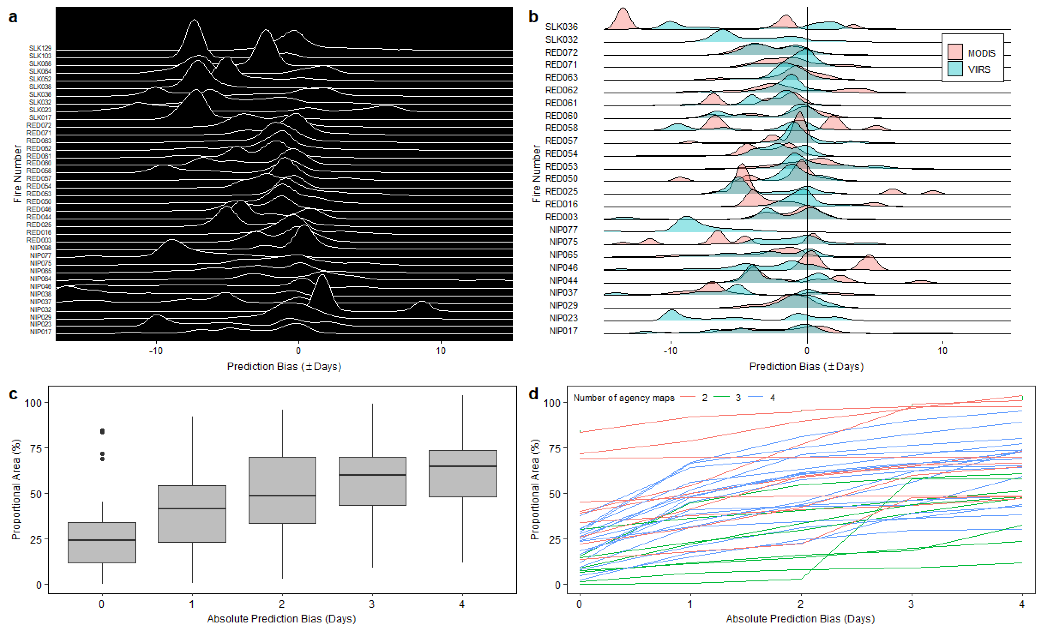
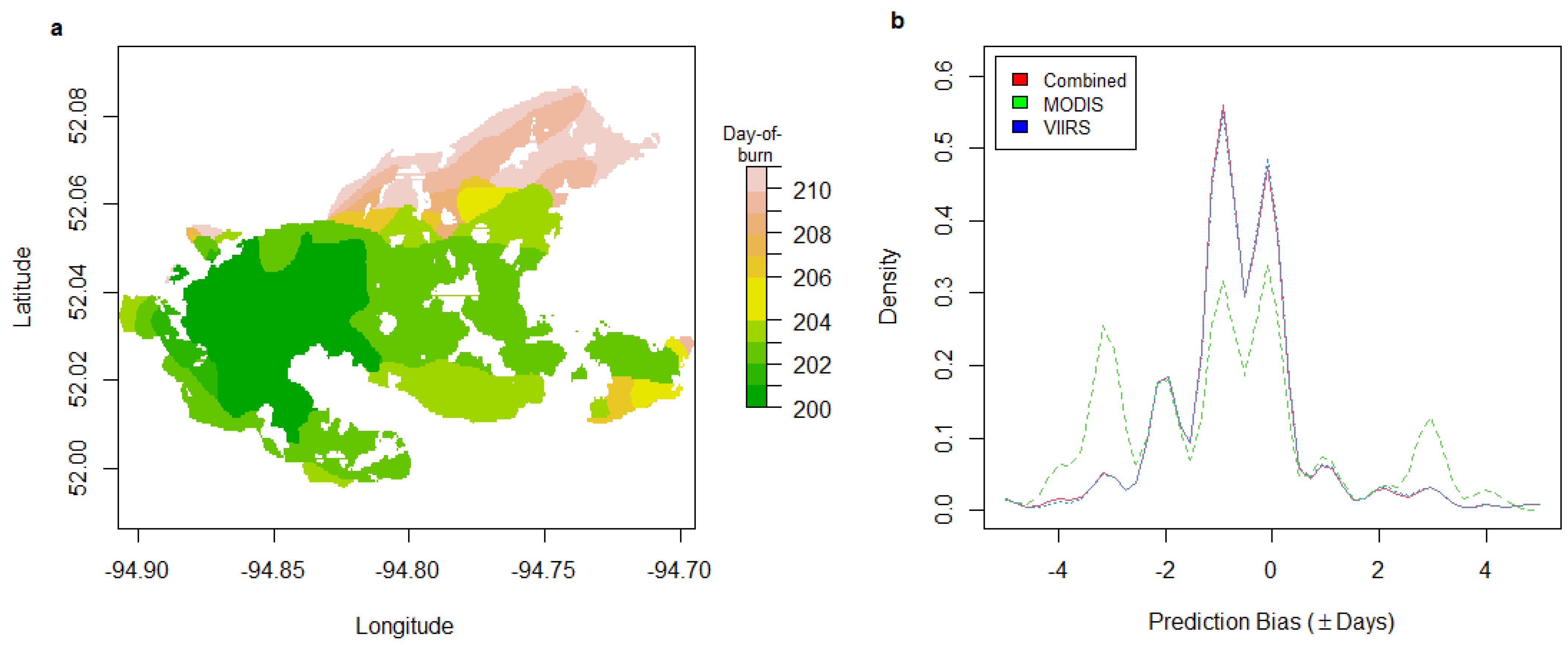
3.1. Ordinary Kriging

The final sizes of the 37 study fires ranged from 110 to 74,334 ha, with durations ranging from 33 to 96 days (based on the difference between the agency-designated Start Date and Out Date). These fires were taken from a cross section of Ontario fires that occurred between 2012 and 2017 and were large, monitored fires (except four fires that were <200 ha and RED-003-2016, which was suppressed), for which multiple perimeter maps were available in digital format. After omitting active fire detections with a confidence value <40%, 26 wildfires were detected at some point over their duration using MODIS, whereas 37 wildfires were detected with VIIRS (

Table 2. Descriptive statistics, variogram parameters, and correlation for 37 study fires in Northwestern Ontario, Canada.

Fire Number	Duration	No. of Agency Maps	Fire Area (ha)	Moran’s I	No. of Hotspots		Variogram Parameters			MODIS	VIIRS		Combined
					MODIS	VIIRS	Nugget (days2)	Sill (days2)	Range (km)	r	r	k	r	A	R2	RMSE
RED-050-2012	196–234	6	6956	0.93	34	670	0	14.5	5.7	0.45	0.77	0.38	0.77	0.58	0.59	2.17
RED-053-2012	196–255	9	18,845	0.94	480	1336	0.12	15.5	4.2	0.66	0.71	0.78	0.72	0.05	0.52	2.28
RED-057-2012	189–234	4	2706	0.92	21	182	1.04	37.3	24.9	−0.01	0.38	0	0.35	0.17	0.13	2.02
RED-058-2012	190–234	6	1884	0.98	22	171	0	20.7	2.9	−0.24	0.32	0	0.31	0.38	0.09	4.50
RED-060-2012	184–234	6	2742	0.97	115	694	1.26	124.3	55.0	0.45	0.46	0.70	0.46	0.15	0.21	2.84
RED-061-2012	196–255	6	956	0.93	20	164	2.12	5.2	1.9	0.03	0.47	0.39	0.43	0.00	0.18	2.41
RED-062-2012	195–255	5	1016	0.95	17	94	0	409.0	39.9	0.53	0.78	0.76	0.77	0.48	0.59	2.41
RED-063-2012	195–255	6	3577	0.93	19	407	1.38	115.8	22.9	0.45	0.79	0.34	0.77	0.40	0.59	1.90
RED-071-2012	184–235	10	6085	0.94	24	414	0	204.4	83.1	0.83	0.91	0.84	0.91	0.55	0.82	1.47
RED-072-2012	189–285	8	13,631	0.94	109	1029	0.97	13.6	4.6	0.74	0.71	0.82	0.71	0.56	0.51	1.95
NIP-017-2015	159–228	5	15,827	0.91	37	278	3.51	23.3	7.0	0.57	0.47	0.60	0.49	0.64	0.24	4.09
NIP-023-2015	168–228	3	4067	0.94	3	122	0.38	116.5	70.8	-	0.65	-	-	-	-	-
RED-016-2015	166–226	5	2629	0.96	22	113	1.64	132.1	42.5	0.39	0.83	0.52	0.83	0.69	0.69	2.08
RED-025-2015	175–226	5	2189	0.92	39	109	0	181.3	37.2	0.07	0.83	0.30	0.83	0.00	0.68	2.88
RED-044-2015	177–226	5	1024	0.96	10	102	0	57.0	50.3	0.59	0.89	0.81	0.88	0.73	0.77	2.02
RED-046-2015	177–226	5	333	0.97	3	38	0	22.4	1.31	-	0.83	-	-	-	-	-
RED-003-2016	126–222	8	74,334	0.78	609	526	0.87	208.0	707	0.87	0.64	0.91	0.88	0.70	0.78	2.48
NIP-029-2017	208–270	7	6999	0.92	16	1088	1.01	31.6	8.8	0.79	0.83	0.70	0.83	0.60	0.69	1.80
NIP-032-2017	210–262	2	168	0.97	0	18	18.68	0.5	7.1	-	−0.05	-	-	-	-	-
NIP-037-2017	210–253	4	3915	0.92	8	299	0	21.5	4.2	0.61	0.68	0.60	0.69	0.68	0.47	6.27
NIP-038-2017	210–255	2	205	0.95	0	22	3.29	83.7	5.0	-	0.56	-	-	-	-	-
NIP-046-2017	212–253	2	208	0.93	28	119	0.49	1470.8	187.1	−0.33	0.35	0	0.34	0.00	0.11	1.84
NIP-064-2017	220–262	3	530	0.97	0	60	0	124.3	1.6	-	0.73	-	-	-	-	-
NIP-065-2017	220–253	3	3486	0.96	7	394	4.08	30.6	2.5	0.70	0.74	0	0.73	0.48	0.54	3.41
NIP-075-2017	220–262	6	674	0.95	35	107	9.07	978.1	56.9	−0.01	0.67	0.44	0.69	0.37	0.47	3.13
NIP-077-2017	210–255	2	574	0.95	0	54	2.40	34.7	7.3	-	0.41	-	-	-	-	-
NIP-098-2017	210–255	4	4736	0.93	0	1066	3.51	353.3	80.8	-	0.68	-	-	-	-	-
RED-054-2017	215–276	2	4049	0.93	56	418	4.56	23.3	1.4	0.11	0.28	0.34	0.27	0.17	0.07	1.44
SLK-017-2017	205–261	3	3690	0.64	15	253	1.76	71.7	41.4	−0.01	0.10	0.29	0.10	0.67	0.01	1.35
SLK-032-2017	209–248	2	230	0.96	0	26	0	35.4	0.5	-	0.81	-	-	-	-	-
SLK-036-2017	210–261	4	2230	0.96	14	149	0	20.6	4.3	0.09	0.53	0	0.54	0.42	0.30	5.63
SLK-038-2017	210–261	2	653	0.88	0	76	1.69	64.7	11.4	-	0.37	-	-	-	-	-
SLK-052-2017	215–248	2	1320	0.96	10	88	0	11.9	0.7	0.00	0.46	0.02	0.45	0.29	0.20	2.42
SLK-064-2017	216–248	2	132	0.94	0	15	1.53	5.3	0.7	-	0.72	-	-	-	-	-
SLK-068-2017	217–261	2	510	0.52	0	69	0.37	3.8	11.5	-	−0.01	-	-	-	-	-
SLK-103-2017	226–261	2	110	0.96	0	5	12.25	12.3	0.1	-	0.65	-	-	-	-	-
SLK-129-2017	222–261	2	121	0.98	0	13	0	23.9	0.3	-	−0.07	-	-	-	-	-

, Figure 1). Figure 2 shows the acquisition time and frequency of hotspots used for ordinary kriging. The number of active fire detections varied considerably between MODIS and VIIRS for each fire (Table 2), as did the acquisition time over the 24 h diurnal cycle (Figure 2).

The variogram model parameter estimates for each fire, based on using the combined detection data set as inputs, are presented in Table 2. Sill and range values varied from 0.52 to 1470 days² and 0 to 187 km, respectively; generally, smaller fires produced the highest parameter estimates. Spatial outliers can cause erratic behaviour in a variogram model, which may partially explain some of the exceptionally high parameter estimates that we observed for some smaller fires (e.g., NIP-046-2017 and NIP-075-2017). While we used the spherical variogram model, data exploration revealed that five fires had a slightly better fit with an exponential variogram model (based on the sum of square errors), which indicated the variance in arrival times did not level off at increasing distance for that fire. Many fires seem to have a nugget effect, though several fires had nugget values greater than 0 days², indicating that as hotspots got closer together, variability in arrival times remained high. The nugget value may also indicate the input data were sparse for that fire. Had the data been pre-screened for first detection, the variability in arrival times would not have been properly characterized (see Section 2.3).

When compared to the agency burned area maps, day-of-burn estimates from MODIS generally had lower r values than VIIRS-based estimates, except for three fires (RED-072-2012, NIP-017-2015, and RED-003-2016; Table 2). The r values from the combined data ranged from 0.10 to 0.91, and 14 of the study fires had r > 0.70. Six fires had negative correlation coefficients for either MODIS or VIIRS, indicating that pixel-based matching was very poor between the estimated fire growth from the prediction surfaces and the agency’s progression maps. The R² values from the combined data ranged from 0.01 to 0.82, and the RMSE ranged from 1.444 to 6.265 days.

Cohen’s kappa correlation coefficient indicated highly variable inter-rater reliability between MODIS- and VIIRS-based prediction surfaces, which ranged from 0 to 0.91 (Table 2). Cohen’s kappa values of 0 indicated that progression inferences from the two active fire detection sources were not consistent (e.g., MODIS suggested an east-to-west fire progression, whereas VIIRS suggested a west-to-east progression) for five of the study fires. Agreement between MODIS and VIIRS prediction surfaces was moderate for six wildfires (0.60 < k < 0.79) and strong for four (k > 0.80). Of the study fires, the suppressed wildfire, RED-003-2016, had the highest value of inter-rater reliability (k = 0.91).

3.2. Prediction Bias

Figure 3a presents a summary of the positive and negative biases between the prediction surfaces and the agency burned area maps for the 37 study fires (using combined active fire detections, except when only VIIRS observations were available; Table 2). An overall trend towards negative prediction bias (i.e., the predicted day of burn was earlier than the agency mapping date) for most fires was a direct consequence of the quasi-validation comparing two maps that are functionally different: the prediction was based on instantaneous hotspots, while the agency recorded burned area maps were updated sometime afterwards and thus captured “burned by dates”. A relatively minor positive prediction bias may be attributable to the known problem that the timestamp associated with an active fire detection does not necessarily record the fire’s first arrival in that cell (instead may record some later time), resulting in a predicted burn date that is later than the agency burn date. Alternatively, the positive prediction bias may be because the agency acquired maps when hotspots were not detectable due to minimum fire size/temperature threshold criteria not being met or a temporarily obstructed view of the fire, whether partially or entirely, from clouds and smoke. Figure 3b shows the areal proportion of matching pixels from the separate MODIS and VIIRS prediction surfaces with agency burned area maps for individual fires when both detection types were present (Table 2). Based on qualitative visual inspection, greater pixel-based matching and accuracy with the agency burned area maps were often achieved using VIIRS-based predictions than using MODIS, but not for every study fire.

The prediction bias results are presented in Figure 3c as a box-and-whiskers plot of the differences between the prediction surface from combined detections and agency burned area maps. About 28% of the predictions were exact matches with agency maps (i.e., the difference of 0 days), 42% were within plus or minus one day, and 50% were within plus or minus two days. Overall, our quasi-validation results of hotspot-based predictions for 37 study fires in Ontario displayed a gradual levelling-off of spatial-temporal accuracy; about 63% of the area of all fires were accurately predicted to within plus or minus four days. Figure 3d displays the difference in burn date results for individual fires, grouped by the number of times the agency recorded a burned area map. Fires with two agency update maps were generally smaller and shorter in duration, and thus, some of those fires showed exceptionally good pixel-based matches and accuracy; fires with three updates showed relatively worse accuracy, but they improved with additional burned area updates.

Figure 3 and

Table 3. Summary of Northwestern Ontario study fires mapped by agency before first active fire detection using MODIS or VIIRS.

Fire Number	Start Date	Agency Map Date	Fire Size	First MODIS	First VIIRS	Difference (Days)
RED-057-2012	189	200	125	203	-	3
RED-058-2012	190	200–204	195, 268, 168 *, 529	205	-	5
NIP-017-2015	159	164	263	174	170	10, 6
RED-025-2015	175	176	53	185	-	9
RED-044-2015	177	184	67	192	186	8, 2
NIP-046-2015	212	234	84	238	-	4
SLK-036-2017	210	212	261	-	220	8
SLK-052-2017	215	219	104	223	-	4
NIP-032-2017	210	211	31	-	219	8
SLK-038-2017	210	217	15	-	220	3
SLK-129-2017	222	225	599	-	226	1

* Size decreases due to a more accurate map of fire perimeter.

show that for 11 of the study fires (~30% of fires), the agency’s first burned area map was acquired one or more days before the first active fire detection. Moreover, both the MODIS and VIIRS data had instances in which a wildfire was not detected using the satellite-borne sensor until it was several hundred hectares in size.

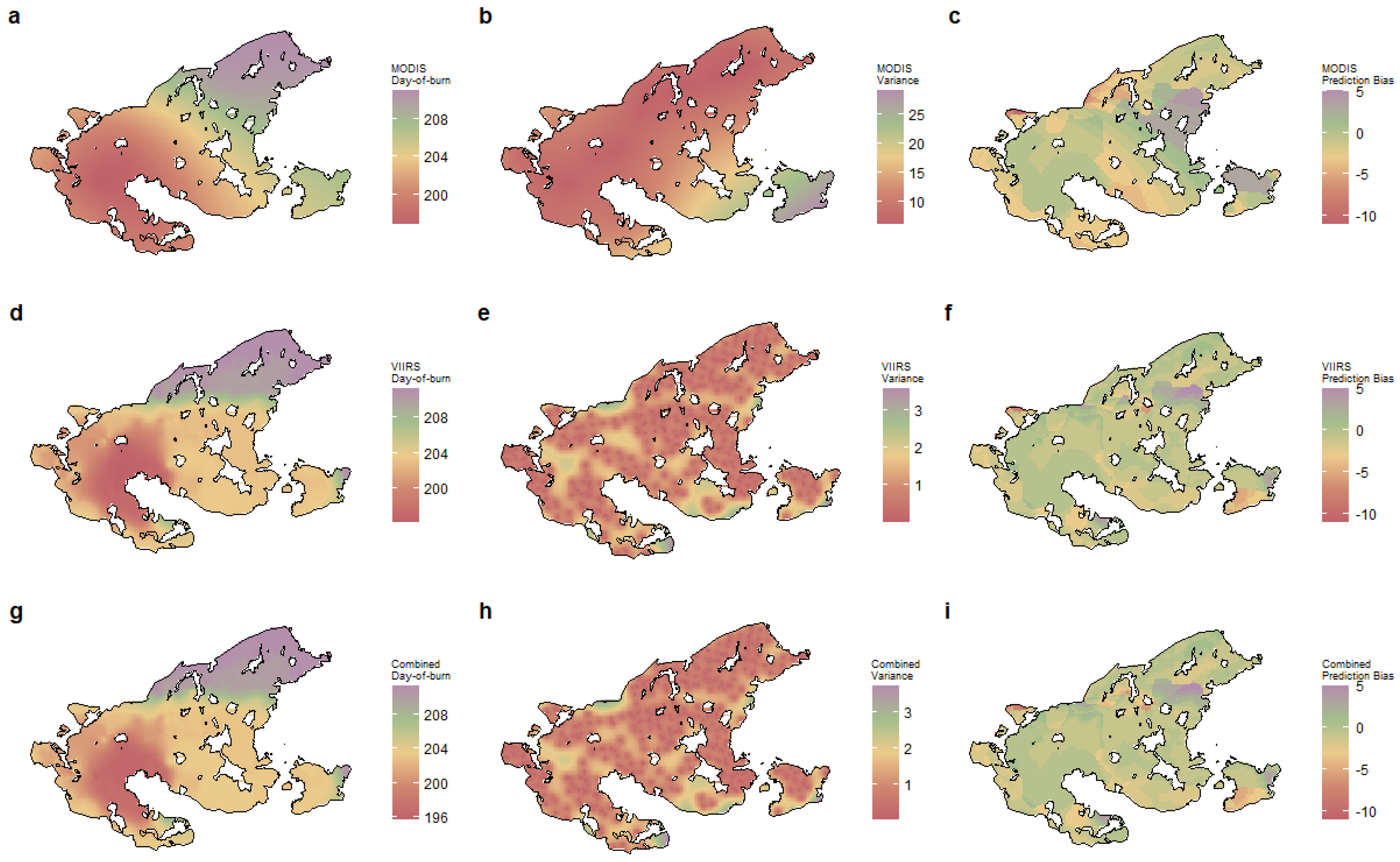
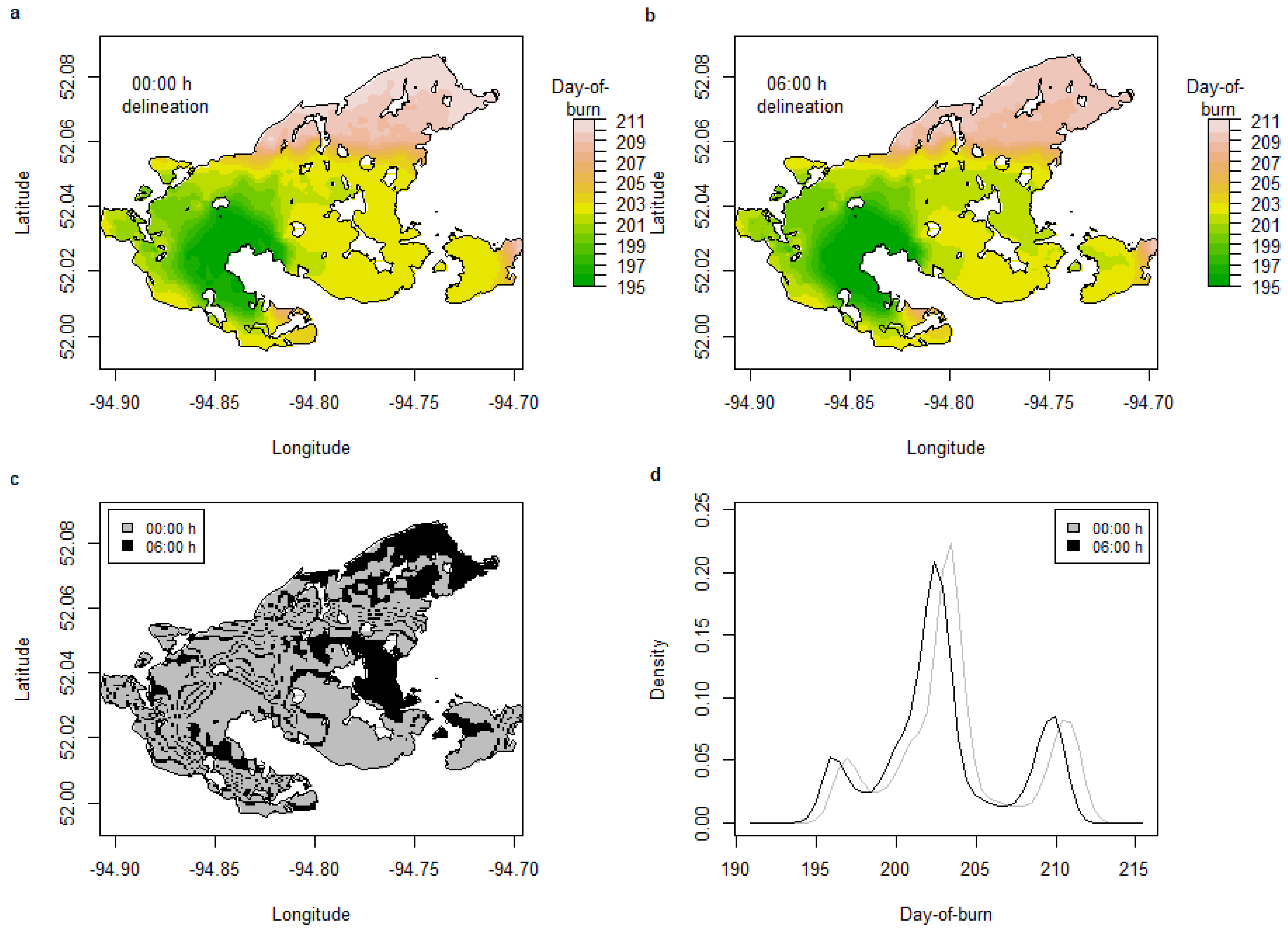
3.3. Wildfire Case Study: RED-071-2012

Here, we focus on one monitored wildfire for which the agency recorded burned area updates over ten days as a case study. RED-071-2012 was a lightning-caused wildfire estimated to have started on day-of-year 184 (2 July 2012) based on the Daily Fire Operations Support System fire archive records [85]; however, the first active fire detections were not observed using MODIS or VIIRS products until day-of-year 196 (14 July 2012). When the fire was observed by aircraft personnel about two weeks later (day-of-year 199 or 17 July 2012), its estimated size was 400 ha.

Figure 4 presents the kriging predictions and kriging standard errors for the burn date interpolation of RED-071-2012. Based on inference from the kriging prediction surfaces in Figure 4, it appears that this wildfire grew outwards in all directions for the first few days, and its southeastern perimeter extinguished after burning to a lakeshore. A significant growth event occurred on day-of-year 204, when the burned area more than doubled and the fire spotted across a different lake. The fire grew towards the northeast at a relatively slower daily average spread rate and finally extinguished naturally.

Visual inspection of the MODIS-based prediction surface (r = 0.83) for RED-071-2012 shows some evidence of the bull’s eye effect (concentric areas of similar values near known data points; Figure 4a). The VIIRS-based prediction surface (r = 0.91) may also display this effect to some degree, but it depicts a very different series of growth events on day-of-year 204 and 205. The combined prediction surface (r = 0.91) did not have an increased r value compared with VIIRS only; however, the kriging standard error maps indicated that the error was minimized with the combined data set (Figure 4h). Generally, the standard error is higher in areas with few active fire detections, and the error increases with increasing distance between the prediction pixel and the hotspot (Figure 4, variance plots in the second column). Based on the density plot of prediction bias (Figure 5), the VIIRS-based predictions seem to better match the agency-mapped data than the MODIS-based predictions.

Figure 6 displays burn period delineation results for RED-071-2012 to illustrate how the time changed the final predicted burn date (grey cell = no change in predicted burn date between 0:00 and 06:00 h; green cell = burn date changed using 06:00 h). The 06:00 h delineation showed the fire perimeter growth extending further to the east on day-of-year 202 and 203 (shown in yellow and light green) and revealed a spotting event that occurred overnight on the southeast portion of the fire. Predictably, the distribution of burn pixels shifted to the left (towards earlier satellite burn date estimates) using the 06:00 h delineation.

4. Discussion

4.1. Fire Progression Mapping

This study is the first quasi-validation of day-of-burn mapping for wildfires occurring in the Canadian boreal forest region. We examined intra-fire spread reconstruction in terms of the daily growth that could be estimated using data recorded using two satellite-based active fire detection sensors and found that by using the combined data set of MODIS and VIIRS detections, nearly half of every study fire’s burned area was accurately predicted to within one day of the actual day it burned (Figure 3). However, the day-of-burn mapping results varied widely among individual fires, and although VIIRS did detect all studied fires, relying solely on VIIRS detections did not always result in more accurate estimates of burn dates than MODIS detections (Table 2).

The variogram parameter estimates were similar to the ranges of values reported by Veraverbeke et al. [34], who also used a spherical variogram model, although they found an average areal proportion of matching pixels of 34% using nine validation fires from the Southwestern United States. The MODIS MCD64A1 burn date product [86] was also validated in that study and was found to have correctly identified the day of burning for 20% of pixels that were burned, slightly less than the results we found using combined active fire detections (28% of pixels were exact matches averaged across our 37 study fires).

Comparatively worse day-of-burn mapping performance is expected for fires that burn less than <~500 ha [35]; increased accuracy has been observed for larger fires that burn longer [38]. Our study results resolve a knowledge gap with respect to how well geospatial interpolation techniques perform for wildfires at the low end of the large fire size distribution (fire size classes E and F: 100–1000 ha and 1000-10,000 ha, respectively) [87]. Three fires that were >10,000 ha (class G) had higher r values using MODIS than VIIRS.

Our study demonstrates the value of recognizing the potential for significant growth events to occur overnight. A visual comparison of the discrepancy in burn dates between the 00:00 and 06:00 h delineations in Figure 6c indicated that a significant growth event occurred overnight on RED-071-2012, which would be attributed to different burn dates depending on the delineation choice. As for the most appropriate delineation of 24 h burn periods, the minimum fire spread activity expected on a day with a typical weather pattern occurs near or just after sunrise, when the air temperature is at a minimum, relative humidity is at a maximum, and wind speed is relatively low [88]. Since many of the studies that use day-of-burn information are explorations of the predictive ability of fire weather, behaviour, and growth models, the selection of 06:00 h (versus 00:00 h) as the end of the previous burn day should associate growth somewhat more accurately with the correct daily fire weather observations. Though we chose to explore 24 h delineations of burned area, it is possible to further divide burn periods into sub-daily periods that are 8 or 12 h (e.g., morning, evening, or overnight periods of burning) and relate each period to hourly weather observations.

4.2. Limitations

Our study highlights several limitations of the independent data set used for quasi-validation and spatial statistical analysis.

Studies that compare burn date interpolation maps to agency-based observations are inherently limited by the frequency and type of observations collected for quasi-validation, and indeed, any future meta-analysis would seemingly be confounded by such differences. Results shown in Figure 3d suggested that greater accuracy was often found when more agency update maps were available; specifically, four or more burned area updates generally demonstrated the best pixel-based matching. Since the accuracy results presented in Figure 3 were sensitive to the quality of the independent data used for quasi-validation, a consideration for future analysis might be to normalize or scale the number of update maps by the fire duration to better reflect the influence of observational frequency on the potential uncertainty of the agency maps. Veraverbeke et al. (2014) and Scaduto et al. (2020) reported somewhat higher accuracy between their interpolated day-of-burn maps and agency perimeters from US Forest Service National Infrared Operations, probably because their validation data type consisted of nearly complete nighttime thermal infrared imagery of perimeters acquired nightly between 22:00 h and 02:00 h for the duration of each fire [23,67]. Additionally, our study results were limited by a lack of information about the exact time of day that the agency acquired the burned area update map. Uncertainty would be reduced with consistent records of acquisition time for each agency burned area map and would presumably improve the accuracy of the results of future quasi-validation work. This temporal criterion may inform future fire mapping protocols adopted by Canadian fire agencies; however, it would require considerable effort and coordination to standardize the protocols for fire perimeter mapping.

The ordinary kriging assumptions of stationarity (mean and variance of values are constant) and isotropy (uniform in all directions) [65] are likely violated to some degree when interpolating fire growth. Firstly, for the stationarity assumption to be met, fire spread (or arrival time) would have to be constant across the entire burned area and for the entire multiday lifetime of the fire. Secondly, the assumption of isotropy is not met because spread is not uniform in all directions but instead is highly dependent on wind direction; therefore, anisotropic approaches to kriging are likely more suitable [89]. Universal kriging might be used as an alternative because it allows spread value means to differ among locations within the fire perimeter while assuming a constant variance.

4.3. Future Research

Since the overarching goal is to reduce uncertainty in estimates of burn dates in a final fire polygon, the challenge is to create a workflow processing framework useful for combining disparate remotely sensed data types [41]. While active fire detections have long been recognized as a source of data to improve our understanding of wildfire processes, neither MODIS nor VIIRS data can be used to produce accurate estimates of the exact arrival time at or duration of burning in a pixel. Future investigation should explore whether the kriging prediction surface based on combined MODIS and VIIRS hotspots is improved by cross-referencing with complementary wildfire remote sensing products, such as burn scar data [39], synthetic aperture radar data [40], and geostationary satellite active fire detection data [90].

Future explorations of burn date mapping should focus on comparing accuracy results across a latitudinal gradient as well as among fire-prone ecoregions. The former is relevant to the boreal forest because the overlapping tracks of polar-orbiting satellites near the Earth’s poles produce more frequent active fire detection coverage at higher latitudes. While consecutive active fire acquisitions near the equator occur twice per day (morning and nighttime overpasses), acquisitions near the Arctic may occur within only a couple of hours [61]. The implication for the Canadian boreal forest is that the additional hotspots observed on wildfires burning at higher latitudes may produce more accurate progression maps. The latter is relevant because the accuracy of mapping results for an individual fire is affected by terrain, species composition, rates of spread, etc., and each of these varies considerably among Canadian ecoregions.

Active fire products are often touted as being a consistent, unbiased means to observe fire dynamics over regions that are vast, remote, and diverse (ecologically, politically, and economically) [29,91,92]; however, as evidenced by our quasi-validation results, it is not guaranteed nor is it realistic to expect that a day-of-burn map is perfectly accurate. Because an inaccurate day-of-burn map would likely add substantial confounding noise to any burn date data set, it seems apt to explore the minimum input data needs (e.g., minimum density of hotspots per fire) to retain a candidate day-of-burn map for subsequent statistical analyses. Using Cohen’s kappa correlation coefficient to compare the prediction surfaces produced using MODIS and VIIRS separately provides some estimate of coherence between the active fire detections from the two sensors, and this or other confidence measures might be used as a screening criterion for candidate fire selection. Re-examination of the research questions outlined in Table 1 with day-of-burn maps based on a combination of MODIS and VIIRS detections may reveal patterns that were previously statistically undetectable due to relying on progression inferences from only one instrument or analyzing all reconstruction maps regardless of their accuracy.

Advancements in mapping the daily area burned by fires should, in turn, improve the accuracy of estimates from bottom-up inventories of wildfire emissions. Fire progression maps allow weather, fuel moisture, and burning conditions (e.g., combustion completeness, and emissions factors) to vary temporally instead of assuming a fixed condition for the entire fire event [34]. Thus, our burn date interpolation method might be used to investigate the extent to which emissions estimates vary based on the MODIS, VIIRS, and combined active fire detection data sets.

5. Conclusions

In summary, we investigated how the prediction accuracy of daily fire progression maps could be improved by combining two sources of satellite-based active fire detection data. Our quasi-validation, using an independent data set of 37 wildfires that occurred in Ontario’s boreal forest region, resulted in accurate estimates of the date of burning for nearly half of the area burned within one day using the combined data set of MODIS and VIIRS active fire detections. Separately, MODIS and VIIRS could accurately map the progression for most of the study fires; however, 11 fires were not detected via MODIS. While VIIRS tended to be more accurate than MODIS, this was not the case for three of the largest fires studied. Importantly, the two data sets did not always give the same progression trend according to our assessment of inter-rater reliability. Of the study fires, the suppressed wildfire, RED-003-2016, had the highest value of inter-rater reliability (k = 0.91). Our study results resolve a knowledge gap with respect to how well the geospatial interpolation technique of ordinary kriging performs for wildfires at the low end of the large fire size distribution. VIIRS is capable of mapping smaller fires than MODIS, though evidently, accuracy diminishes as fire size decreases. The presence of spatial autocorrelation is a relevant statistical consideration for any validation of burn date mapping techniques, as performance assessments that ignore this issue will likely overestimate agreement. Our approach may be used to generate a geodatabase of historical fire progression reconstruction maps, to study environmental controls on fire behaviour and fire effects, or to independently validate predictions from a fire growth model.

References

1. Wooster, M.J.; Zhang, Y.H. Boreal Forest Fires Burn Less Intensely in Russia than in North America. Geophys. Res. Lett. 2004, 31, 2–4. [Google Scholar] [CrossRef]
2. French, N.H.F.; Goovaerts, P.; Kasischke, E.S. Uncertainty in Estimating Carbon Emissions from Boreal Forest Fires. J. Geophys. Res. Atmos. 2004, 109, D14S08. [Google Scholar] [CrossRef]
3. Randerson, J.T.; Liu, H.; Flanner, M.G.; Chambers, S.D.; Jin, Y.; Hess, P.G.; Pfister, G.; Mack, M.C.; Treseder, K.K.; Welp, L.R.; et al. The Impact of Boreal Forest Fire on Climate Warming. Science 2006, 314, 1130–1132. [Google Scholar] [CrossRef]
4. Adams, M.A. Mega-Fires, Tipping Points and Ecosystem Services: Managing Forests and Woodlands in an Uncertain Future. For. Ecol. Manag. 2013, 294, 250–261. [Google Scholar] [CrossRef]
5. Flannigan, M.D.; Vonder Haar, T. Forest Fire Monitoring Using NOAA Satellite AVHRR. Can. J. For. Res. 1986, 16, 975–982. [Google Scholar] [CrossRef]
6. Ressl, R.; Lopez, G.; Cruz, I.; Colditz, R.R.; Schmidt, M.; Ressl, S.; Jiménez, R. Operational Active Fire Mapping and Burnt Area Identification Applicable to Mexican Nature Protection Areas Using MODIS and NOAA-AVHRR Direct Readout Data. Remote Sens. Environ. 2009, 113, 1113–1126. [Google Scholar] [CrossRef]
7. Hawbaker, T.J.; Vanderhoof, M.K.; Beal, Y.-J.; Takacs, J.D.; Schmidt, G.L.; Falgout, J.T.; Williams, B.; Fairaux, N.M.; Caldwell, M.K.; Picotte, J.J.; et al. Mapping Burned Areas Using Dense Time-Series of Landsat Data. Remote Sens. Environ. 2017, 198, 504–522. [Google Scholar] [CrossRef]
8. Natural Resources Canada FireMARS. Available online: https://www.nrcan.gc.ca/our-natural-resources/forests/wildland-fires-insects-disturbances/fire-monitoring-reporting-tool/13159 (accessed on 10 January 2017).
9. Natural Resources Canada Canadian Wildland Fire Information System. Available online: http://cwfis.cfs.nrcan.gc.ca/background/summary/fwi (accessed on 10 January 2017).
10. San-Miguel-Ayanz, J.; Barbosa, P.; Liberta, G.; Schmuck, G.; Schulte, E.; Bucella, P. The European Forest Fire Information System: A European Strategy towards Forest Fire Management. In Proceedings of the Third International Wildland Fire Conference, Sydney, Australia, 3–6 October 2003. [Google Scholar]
11. Copernicus Emergency Management Service Global Wildfire Information System (GWIS). Available online: http://gwis.jrc.ec.europa.eu/ (accessed on 10 January 2017).
12. Robinson, J. Fire from Space: Global Fire Evaluation Using Infrared Remote Sensing. Int. J. Remote Sens. 1991, 12, 3–24. [Google Scholar] [CrossRef]
13. Dozier, J. A Method for Satellite Identification of Surface Temperature Fields of Subpixel Resolution. Remote Sens. Environ. 1981, 11, 221–229. [Google Scholar] [CrossRef]
14. Giglio, L.; Kendall, J.D.; Justice, C.O. Evaluation of Global Fire Detection Algorithms Using Simulated AVHRR Infrared Data. Int. J. Remote Sens. 1999, 20, 1947–1985. [Google Scholar] [CrossRef]
15. Li, Z.; Kaufman, Y.; Ichoku, C.; Fraser, R.; Trishchenko, A.; Giglio, L.; Jin, J.; Yu, X. A Review of AVHRR-Based Active Fire Detection Algorithms: Principles, Limitations, and Recommendations. In Global and Regional Vegetation Fire Monitoring from Space: Planning a Coordinated International Effort; Ahern, F., Goldammer, J., Justice, C., Eds.; SPB Academic Publishing: The Hague, The Netherlands, 2001; pp. 199–225. [Google Scholar]
16. Ichoku, C.; Kaufman, Y.J.; Giglio, L.; Li, Z.; Fraser, R.H.; Jin, J.-Z.; Park, W.M. Comparative Analysis of Daytime Fire Detection Algorithms Using AVHRR Data for the 1995 Fire Season in Canada: Perspective for MODIS. Int. J. Remote Sens. 2003, 24, 1669–1690. [Google Scholar] [CrossRef]
17. Li, Z.; Fraser, R.; Jin, J.; Abuelgasim, A.A.; Csiszar, I.; Gong, P.; Pu, R.; Hao, W. Evaluation of Algorithms for Fire Detection and Mapping across North America from Satellite. J. Geophys. Res. Atmos. 2003, 108, 4076. [Google Scholar] [CrossRef]
18. Wooster, M. Fire Radiative Energy for Quantitative Study of Biomass Burning: Derivation from the BIRD Experimental Satellite and Comparison to MODIS Fire Products. Remote Sens. Environ. 2003, 86, 83–107. [Google Scholar] [CrossRef]
19. Wooster, M.J.; Roberts, G.; Perry, G.L.W.; Kaufman, Y.J. Retrieval of Biomass Combustion Rates and Totals from Fire Radiative Power Observations: FRP Derivation and Calibration Relationships between Biomass Consumption and Fire Radiative Energy Release. J. Geophys. Res. Atmos. 2005, 110, D24311. [Google Scholar] [CrossRef]
20. Flasse, S.P.; Ceccato, P. A Contextual Algorithm for AVHRR Fire Detection. Int. J. Remote Sens. 1996, 17, 419–424. [Google Scholar] [CrossRef]
21. Arino, O.; Simon, M.; Piccolini, I.; Rosaz, J.-M. The ERS-2 ATSR-2 World Fire Atlas and the ERS-2 ATSR-2 World Burnt Surface Atlas Projects. In Proceedings of the 8th ISPRS Conference on Physical Measurement & Signatures in Remote Sensing, Aussois, France, 8–12 January 2001. [Google Scholar]
22. Kaufman, Y.J.; Justice, C.O.; Flynn, L.P.; Kendall, J.D.; Prins, E.M.; Giglio, L.; Ward, D.E.; Menzel, W.P.; Setzer, A.W. Potential Global Fire Monitoring from EOS-MODIS. J. Geophys. Res. Atmos. 1998, 103, 32215–32238. [Google Scholar] [CrossRef]
23. Csiszar, I.; Schroeder, W.; Giglio, L.; Ellicott, E.; Vadrevu, K.P.; Justice, C.O.; Wind, B. Active Fires from the Suomi NPP Visible Infrared Imaging Radiometer Suite: Product Status and First Evaluation Results. J. Geophys. Res. Atmos. 2014, 119, 803–816. [Google Scholar] [CrossRef]
24. Schroeder, W.; Oliva, P.; Giglio, L.; Csiszar, I.A. The New VIIRS 375 m Active Fire Detection Data Product: Algorithm Description and Initial Assessment. Remote Sens. Environ. 2014, 143, 85–96. [Google Scholar] [CrossRef]
25. Agee, J.K. Fire Regimes and Approaches for Determining Fire History. In The Use of Fire in Forest Restoration; Hardy, C., Arno, S., Eds.; General Technical Report INT-GTR-341; U.S. Department of Agriculture, Forest Service, Intermountain Research Station: Ogden, UT, USA, 1996; pp. 12–13. [Google Scholar]
26. Yocom Kent, L.L. An Evaluation of Fire Regime Reconstruction Methods; Working Papers in Southwestern Ponderosa Pine Forest Restoration #32; Southwest Fire Science Consortium and Ecological Restoration Institute, Northern Arizona University: Flagstaff, AZ, USA, 2014; 15p. [Google Scholar]
27. Harrison, S.P.; Prentice, I.C.; Bloomfield, K.J.; Dong, N.; Forkel, M.; Forrest, M.; Ningthoujam, R.K.; Pellegrini, A.; Shen, Y.; Baudena, M.; et al. Understanding and Modelling Wildfire Regimes: An Ecological Perspective. Environ. Res. Lett. 2021, 16, 125008. [Google Scholar] [CrossRef]
28. Kasischke, E.S.; Hewson, J.H.; Stocks, B.; van der Werf, G.; Randerson, J. The Use of ATSR Active Fire Counts for Estimating Relative Patterns of Biomass Burning—A Study from the Boreal Forest Region. Geophys. Res. Lett. 2003, 30, 2–5. [Google Scholar] [CrossRef]
29. Loboda, T.V.; Csiszar, I.A. Reconstruction of Fire Spread within Wildland Fire Events in Northern Eurasia from the MODIS Active Fire Product. Glob. Planet. Chang. 2007, 56, 258–273. [Google Scholar] [CrossRef]
30. Ester, M.; Kriegel, H.P.; Sander, J.; Xu, X. A Density-Based Algorithm for Discovering Clusters in Large Spatial Databases with Noise. In Proceedings of the Second Conference on Knowledge Discovery and Data Mining, Portland, OR, USA, 2–4 August 1996; AAAI Press: Portland, OR, USA, 1996; Volume 2, pp. 226–231. [Google Scholar]
31. de Groot, W.J.; Landry, R.; Kurz, W.A.; Anderson, K.R.; Englefield, P.; Fraser, R.H.; Hall, R.J.; Banfield, E.; Raymond, D.A.; Decker, V.; et al. Estimating Direct Carbon Emissions from Canadian Wildland Fires. Int. J. Wildland Fire 2007, 16, 593–606. [Google Scholar] [CrossRef]
32. Kasischke, E.S.; Hoy, E.E. Controls on Carbon Consumption during Alaskan Wildland Fires. Glob. Chang. Biol. 2012, 18, 685–699. [Google Scholar] [CrossRef]
33. Thorsteinsson, T.; Magnusson, B.; Gudjonsson, G. Large Wildfire in Iceland in 2006: Size and Intensity Estimates from Satellite Data. Int. J. Remote Sens. 2011, 32, 17–29. [Google Scholar] [CrossRef]
34. Veraverbeke, S.; Sedano, F.; Hook, S.J.; Randerson, J.T.; Jin, Y.; Rogers, B.M. Mapping the Daily Progression of Large Wildland Fires Using MODIS Active Fire Data. Int. J. Wildland Fire 2014, 23, 655–667. [Google Scholar] [CrossRef]
35. Parks, S.A. Mapping Day-of-Burning with Coarse-Resolution Satellite Fire-Detection Data. Int. J. Wildland Fire 2014, 23, 215–223. [Google Scholar] [CrossRef]
36. Giglio, L.; Schroeder, W.; Justice, C.O. The Collection 6 MODIS Active Fire Detection Algorithm and Fire Products. Remote Sens. Environ. 2016, 178, 31–41. [Google Scholar] [CrossRef]
37. Loboda, T.; Hall, J. ABoVE: Wildfire Date of Burning within Fire Scars across Alaska and Canada, 2001–2015. Oak Ridge National Laboratory Distributed Active Archive Center for Biogeochemical Dynamics: Oak Ridge, TN, USA. Available online: https://doi.org/10.3334/ORNLDAAC/1559 (accessed on 10 January 2017).
38. Scaduto, E.; Chen, B.; Jin, Y. Satellite-Based Fire Progression Mapping: A Comprehensive Assessment for Large Fires in Northern California. IEEE J. Sel. Top. Appl. Earth Obs. Remote Sens. 2020, 13, 5102–5114. [Google Scholar] [CrossRef]
39. Crowley, M.A.; Cardille, J.A.; White, J.C.; Wulder, M.A. Multi-Sensor, Multi-Scale, Bayesian Data Synthesis for Mapping within-Year Wildfire Progression. Remote Sens. Lett. 2019, 10, 302–311. [Google Scholar] [CrossRef]
40. Ban, Y.; Zhang, P.; Nascetti, A.; Bevington, A.R.; Wulder, M.A. Near Real-Time Wildfire Progression Monitoring with Sentinel-1 SAR Time Series and Deep Learning. Sci. Rep. 2020, 10, 1322. [Google Scholar] [CrossRef]
41. Lasko, K. Incorporating Sentinel-1 SAR Imagery with the MODIS MCD64A1 Burned Area Product to Improve Burn Date Estimates and Reduce Burn Date Uncertainty in Wildland Fire Mapping. Geocarto Int. 2021, 36, 340–360. [Google Scholar] [CrossRef]
42. Benali, A.; Russo, A.; Sá, A.; Pinto, R.; Price, O.; Koutsias, N.; Pereira, J. Determining Fire Dates and Locating Ignition Points With Satellite Data. Remote Sens. 2016, 8, 326. [Google Scholar] [CrossRef]
43. Andela, N.; Morton, D.C.; Giglio, L.; Paugam, R.; Chen, Y.; Hantson, S.; van der Werf, G.R.; Randerson, J.T. The Global Fire Atlas of Individual Fire Size, Duration, Speed, and Direction. Earth Syst. Sci. Data 2018, 11, 529–552. [Google Scholar] [CrossRef]
44. Artés, T.; Oom, D.; de Rigo, D.; Durrant, T.H.; Maianti, P.; Libertà, G.; San-Miguel-Ayanz, J. A Global Wildfire Dataset for the Analysis of Fire Regimes and Fire Behaviour. Sci. Data 2019, 6, 296. [Google Scholar] [CrossRef] [PubMed]
45. Humber, M.; Zubkova, M.; Giglio, L. A Remote Sensing-Based Approach to Estimating the Fire Spread Rate Parameter for Individual Burn Patch Extraction. Int. J. Remote Sens. 2022, 43, 649–673. [Google Scholar] [CrossRef]
46. Collins, B.M.; Kelly, M.; van Wagtendonk, J.W.; Stephens, S.L. Spatial Patterns of Large Natural Fires in Sierra Nevada Wilderness Areas. Landsc. Ecol. 2007, 22, 545–557. [Google Scholar] [CrossRef]
47. Collins, B.M.; Miller, J.D.; Thode, A.E.; Kelly, M.; Van Wagtendonk, J.W.; Stephens, S.L. Interactions among Wildland Fires in a Long-Established Sierra Nevada Natural Fire Area. Ecosystems 2009, 12, 114–128. [Google Scholar] [CrossRef]
48. Thompson, J.R.; Spies, T.A. Factors Associated with Crown Damage Following Recurring Mixed-Severity Wildfires and Post-Fire Management in Southwestern Oregon. Landsc. Ecol. 2010, 25, 775–789. [Google Scholar] [CrossRef]
49. Birch, D.S.; Morgan, P.; Kolden, C.A.; Hudak, A.T.; Smith, A.M.S. Is Proportion Burned Severely Related to Daily Area Burned? Environ. Res. Lett. 2014, 9, 064011. [Google Scholar] [CrossRef]
50. Billmire, M.; French, N.H.F.; Loboda, T.; Owen, R.C.; Tyner, M. Santa Ana Winds and Predictors of Wildfire Progression in Southern California. Int. J. Wildland Fire 2014, 23, 1119–1129. [Google Scholar] [CrossRef]
51. Wang, X.; Parisien, M.; Flannigan, M.D.; Parks, S.A.; Anderson, K.R.; Little, J.M.; Taylor, S.W. The Potential and Realized Spread of Wildfires across Canada. Glob. Chang. Biol. 2014, 20, 2518–2530. [Google Scholar] [CrossRef] [PubMed]
52. Parks, S.A.; Holsinger, L.M.; Miller, C.; Nelson, C.R. Wildland Fire as a Self-Regulating Mechanism: The Role of Previous Burns and Weather in Limiting Fire Progression. Ecol. Appl. 2015, 25, 1478–1492. [Google Scholar] [CrossRef] [PubMed]
53. Whitman, E.; Parisien, M.-A.; Thompson, D.K.; Hall, R.J.; Skakun, R.S.; Flannigan, M.D. Variability and Drivers of Burn Severity in the Northwestern Canadian Boreal Forest. Ecosphere 2018, 9, e02128. [Google Scholar] [CrossRef]
54. Baysal, I.; Ouellette, M.; Antoszek, J. Red Lake 084 of 2011: A Reconnaissance Survey of a Large Boreal Wildfire; Forest Research Information Paper 177; Ministry of Natural Resources, Ontario Forest Research Institute: Sault Ste. Marie, ON, Canada, 2011; 91p.
55. Beck, J.A.; Alexander, M.E.; Harvey, S.D.; Beaver, A.K. Forecasting Diurnal Variations in Fire Intensity to Enhance Wildland Firefighter Safety. Int. J. Wildland Fire 2002, 11, 173–182. [Google Scholar] [CrossRef]
56. Hall, R.J.; Skakun, R.S.; Metsaranta, J.M.; Landry, R.; Fraser, R.H.; Raymond, D.; Gartrell, M.; Decker, V.; Little, J. Generating Annual Estimates of Forest Fire Disturbance in Canada: The National Burned Area Composite. Int. J. Wildland Fire 2020, 29, 878–891. [Google Scholar] [CrossRef]
57. R Core Team. R: A Language and Environment for Statistical Computing; R Foundation for Statistical Computing: Vienna, Austria, 2020; Available online: https://www.R--project.org/ (accessed on 10 January 2020).
58. EOSDIS FIRMS Frequently Asked Questions. Available online: earthdata.nasa.gov/faq/firms-faq (accessed on 10 January 2017).
59. Davies, D.K.; Ilavajhala, S.; Wong, M.M.; Justice, C.O. Fire Information for Resource Management System: Archiving and Distributing MODIS Active Fire Data. IEEE Trans. Geosci. Remote Sens. 2009, 47, 72–79. [Google Scholar] [CrossRef]
60. Hantson, S.; Padilla, M.; Corti, D.; Chuvieco, E. Strengths and Weaknesses of MODIS Hotspots to Characterize Global Fire Occurrence. Remote Sens. Environ. 2013, 131, 152–159. [Google Scholar] [CrossRef]
61. Waigl, C.F.; Stuefer, M.; Prakash, A.; Ichoku, C. Detecting High and Low-Intensity Fires in Alaska Using VIIRS I-Band Data: An Improved Operational Approach for High Latitudes. Remote Sens. Environ. 2017, 199, 389–400. [Google Scholar] [CrossRef]
62. Bivand, R.; Rundel, C. Rgeos: Interface to Geometry Engine—Open Source (‘GEOS’). 2019, R Package Version 0.5-2. Available online: https://cran.r--project.org/packages=rgeos (accessed on 10 January 2020).
63. Giglio, L.; Schroeder, W.; Hall, J.V.; Justice, C.O. MODIS Collection 6 Active Fire Product User’s Guide Revision C. 2020. Available online: https://modis-fire.umd.edu/files/MODIS_C6_Fire_User_Guide_C.pdf (accessed on 1 February 2021).
64. Johnston, J.M. Infrared Remote Sensing of Fire Behaviour in Canadian Wildland Forest Fuels. Ph.D. Thesis, King’s College London, London, UK, 2016; 359p. [Google Scholar]
65. Bivand, R.; Pebesma, E.; Gómez-Rubio, V. Applied Spatial Data Analysis with R, 2nd ed.; Springer: New York, NY, USA, 2013; ISBN 9781461476184. [Google Scholar]
66. Chiles, J.-P.; Desassis, N. Fifty Years of Kriging. In Handbook of Mathematical Geosciences: Fifty Years of IAMG; Sagar, D., Cheng, Q., Agterberg, F., Eds.; Springer International Publishing: Berlin, Germany, 2018; pp. 589–612. ISBN 9783319789996. [Google Scholar]
67. Holdaway, M. Spatial Modeling and Interpolation of Monthly Temperature Using Kriging. Clim. Res. 1996, 6, 215–225. [Google Scholar] [CrossRef]
68. Samuel, A.; Morris, M.; Beylerian, E.; Bender-demoll, S.; Weiss, K.; Anderson, S. Sp. 2020, R Package Version 1.4-2. Available online: https://cran.r--project.org/packages=sp (accessed on 1 July 2020).
69. Pebesma, E.; Graeler, B. Gstat. 2019, R Package Version 2.0-3. Available online: https://cran.r--project.org/packages=gstat (accessed on 10 January 2020).
70. Spinu, V.; Grolemund, G.; Wickham, H. Package ‘lubridate’—Make Dealing with Dates a Little Easier. J. Stat. Softw. 2018, 40, 1–25. [Google Scholar]
71. Werth, P.; Potter, B.; Clements, C.; Finney, M.; Goodrick, S.; Alexander, M.; Cruz, M.; Forthofer, J.; McAllister, S. Synthesis of Knowledge of Extreme Fire Behavior: Volume I for Fire Management; General Technical Report PNW-GTR-854; U.S. Department of Agriculture, Forest Service, Pacific Northwest Research Station: Portland, OR, USA, 2011; pp. 1–144.
72. Werth, P.; Potter, B.; Alexander, M.; Cruz, M.; Clements, C.; Finney, M.; Forthofer, J.; Goodrick, S.; Hoffman, C.; Jolly, M.; et al. Synthesis of Knowledge of Extreme Fire Behavior: Volume 2 for Fire Behavior Specialists, Researchers, and Meteorologists; General Technical Report PNW-GTR-891; U.S. Department of Agriculture, Forest Service, Pacific Northwest Research Station: Portland, OR, USA, 2016; pp. 808–2130.
73. Hijmans, R.J.; Van Etten, J.; Sumner, M.; Cheng, J.; Bevan, A.; Bivand, R.; Busetto, L.; Canty, M.; Forrest, D.; Golicher, D.; et al. Raster: Geographic Data Analysis and Modeling. 2019, R Package Version 3.4-5. Available online: https://cran.r--project.org/packages=raster (accessed on 10 January 2020).
74. Wickham, H.; Chang, W.; Henry, L.; Pederson, T. Ggplot2: Elegant Graphics for Data Analysis. 2020, R Package Version 3.3.2. Available online: https://cran.r--project.org/packages=ggplot2 (accessed on 1 July 2020).
75. Wilke, C.O. Ggridges: Ridgeline Plots in “Ggplot2.” 2018, R Package Version 0.5.4. Available online: https://cran.r--project.org/packages=ggridges (accessed on 1 February 2021).
76. Bowman, A.; Azzalini, A. R. Sm: Nonparametric Smoothing Methods. 2018, R Package Version 2.2-5.6. Available online: https://cran.r--project.org/packages=sm (accessed on 10 January 2020).
77. Bataineh, A.L.; Oswald, B.P.; Bataineh, M.; Unger, D.; Hung, I.-K.; Scognamillo, D. Spatial Autocorrelation and Pseudoreplication in Fire Ecology. Fire Ecol. 2006, 2, 107–118. [Google Scholar] [CrossRef]
78. Legendre, P.; Fortin, M.J. Spatial Pattern and Ecological Analysis. Vegetatio 1989, 80, 107–138. [Google Scholar] [CrossRef]
79. Moran, P.A.P. Notes on Continuous Stochastic Phenomena. Biometrika 1950, 37, 17–23. [Google Scholar] [CrossRef] [PubMed]
80. Osorio, F.; Vallejos, R.; Cuevas, F. SpatialPack: Computing the Association Between Two Spatial Processes. arXiv 2016, arXiv:1611.05289. [Google Scholar]
81. Osorio, F.; Vallejos, R.; Cuevas, F.; Mancilla, D. SpatialPack: Tools for Assessment the Association between Two Spatial Processes. 2022, R Package Version 0.4. Available online: https://cran.r--project.org/packages=spatialpack (accessed on 20 October 2022).
82. Cohen, J. A Coefficient of Agreement for Nominal Scales. Educ. Psychol. Meas. 1960, 20, 37–46. [Google Scholar] [CrossRef]
83. Cohen, J. Weighted Kappa: Nominal Scale Agreement Provision for Scaled Disagreement or Partial Credit. Psychol. Bull. 1968, 70, 213–220. [Google Scholar] [CrossRef]
84. Revelle, W. Psych: Procedures for Personality and Psychological Research. 2020, R Package Version 1.9.12.31. Available online: https://cran.r--project.org/package=psych (accessed on 1 October 2021).
85. Martell, D.L.; Kourtz, P.H.; Tithecott, A.; Ward, P.C. The Development and Implementation of Forest Fire Management Decision Support Systems in Ontario, Canada; General Technical Report PSW-GTR-173; U.S. Department of Agriculture, Forest Service, Pacific Northwest Research Station: Berkeley, CA, USA, 1999; pp. 131–142.
86. Giglio, L.; Loboda, T.; Roy, D.P.; Quayle, B.; Justice, C.O. An Active-Fire Based Burned Area Mapping Algorithm for the MODIS Sensor. Remote Sens. Environ. 2009, 113, 408–420. [Google Scholar] [CrossRef]
87. CIFFC Glossary Task Team and Training Working Group. CIFFC Canadian Wildland Fire Glossary; CIFFC: Manitoba, CA, Canada, 2021; 32p. [Google Scholar]
88. Van Wagner, C.E. A Method for Computing Fine Fuel Moisture Content throughout the Diurnal Cycle; Information Report PS-X-69; Canadian Forest Service, Petawawa Forest Experiment Station: Chalk River, ON, Canada, 1977; 15p.
89. Friedland, C.J.; Joyner, T.A.; Massarra, C.; Rohli, R.V.; Treviño, A.M.; Ghosh, S.; Huyck, C.; Weatherhead, M. Isotropic and Anisotropic Kriging Approaches for Interpolating Surface-Level Wind Speeds across Large, Geographically Diverse Regions. Geomat. Nat. Hazards Risk 2017, 8, 207–224. [Google Scholar] [CrossRef]
90. Berman, M.T.; Ye, X.; Thapa, L.H.; Peterson, D.A.; Hyer, E.J.; Soja, A.J.; Gargulinski, E.M.; Csiszar, I.; Schmidt, C.C.; Saide, P.E. Quantifying Burned Area of Wildfires in the Western United States from Polar-Orbiting and Geostationary Satellite Active-Fire Detections. Int. J. Wildland Fire 2023, 32, 665–678. [Google Scholar] [CrossRef]
91. Giglio, L. Characterization of the Tropical Diurnal Fire Cycle Using VIRS and MODIS Observations. Remote Sens. Environ. 2007, 108, 407–421. [Google Scholar] [CrossRef]
92. Giglio, L.; Descloitres, J.; Justice, C.O.; Kaufman, Y.J. An Enhanced Contextual Fire Detection Algorithm for MODIS. Remote Sens. Environ. 2003, 87, 273–282. [Google Scholar] [CrossRef]
Figure 1. Map depicting the day-of-burn prediction surfaces for 37 study fires located in Northwestern Ontario, Canada. Day-of-burn predictions, typically reported using units of day-of-year, have been re-coded to a relativized time format that starts at 0 to represent ignition time. The inset map depicts the location and extent of the study region within Eastern Canada.
Fire 07 00026 g001
Figure 2. Frequency of active fire detection acquisition times over the 24 h diurnal cycle. The grey rectangle depicts the time of peak burning, during which MODIS and VIIRS do not operate over the study area.
Fire 07 00026 g002
Figure 3. Summaries of prediction bias results for 37 fires studied: (a) ridgeline plot summarizing the pixel-based differences in burn date between the kriging prediction surface and the agency maps, (b) comparison of pixel-based differences between the MODIS and VIIRS kriging prediction surfaces, (c) box-and-whiskers plot, and (d) line plot summarizing the areal proportion of matching pixels.
Fire 07 00026 g003
Figure 4. Day-of-burn mapping results for case study fire RED-071-2012: (a) MODIS prediction surface, (b) MODIS variance, (c) MODIS prediction bias, (d) VIIRS prediction surface, (e) VIIRS variance, (f) VIIRS prediction bias, (g) combined prediction surface, (h) combined variance, and (i) combined prediction bias.
Fire 07 00026 g004
Figure 5. Case study fire RED-071-2012: (a) agency burned area update maps and (b) density plot of prediction bias using MODIS, VIIRS, and combined active fire detection data sets.
Fire 07 00026 g005
Figure 6. Comparison of daily burn period delineation using (a) 00:00 h and (b) 06:00 h for case study fire RED-071-2012, (c) map of burn dates (pixels) that differed between the two delineations, and (d) density plot of burn dates for the two delineations.
Fire 07 00026 g006